Regular Language Constrained Sequence Alignment Revisited

Abstract

Imposing constraints in the form of a finite automaton or a regular expression is an effective way to incorporate additional a priori knowledge into sequence alignment procedures. With this motivation, the Regular Expression Constrained Sequence Alignment Problem was introduced, which proposed an O(n²t⁴) time and O(n²t²) space algorithm for solving it, where n is the length of the input strings and t is the number of states in the input non-deterministic automaton. A faster O(n²t³) time algorithm for the same problem was subsequently proposed. In this article, we further speed up the algorithms for Regular Language Constrained Sequence Alignment by reducing their worst case time complexity bound to O(n²t³/log t). This is done by establishing an optimal bound on the size of Straight-Line Programs solving the maxima computation subproblem of the basic dynamic programming algorithm. We also study another solution based on a Steiner Tree computation. While it does not improve the worst case, our simulations show that both approaches are efficient in practice, especially when the input automata are dense.

1. Introduction

Sequence alignment algorithms use a position-independent scoring matrix, but when biologists make an alignment they favor some similarities, depending on their knowledge of the structure and/or the function of the sequences. Various extensions of the Smith-Waterman algorithm (Smith and Waterman, 1981) modify the alignment considerations according to a priori knowledge (Arslan and Egecioglu, 2005; Chen and Chao, 2009; Iliopoulos and Rahman, 2008; Peng and Ting, 2005; Tsai, 2003; Sunyaev et al., 2004; Gotthilf et al., 2008). One kind of a priori knowledge is about shared properties (patterns), which are expected to be preserved by the alignment. Specifically, in protein sequence alignment, it is natural to expect that functional sites be aligned together. Several studies suggested taking into account the patterns, specified by regular expressions, from the PROSITE database (Bairoch, 1993) to guide and constrain protein alignments (Arslan, 2007; Tang et al., 2003), because such patterns may serve as good descriptors of protein families.

Arslan (2007) introduced the Regular Expression Constrained Sequence Alignment Problem. Here, the constraint is given in the form of a non-deterministic finite automaton (NFA). An alignment satisfies the constraint if a segment of it is accepted by the NFA in each aligned sequence (Fig. 1). Arslan's dynamic programming algorithm is based on applying an NFA, with scores assigned to its states, to guide the sequence alignment. This NFA accepts all alignments of the two input strings containing a segment that fits the input regular language. The algorithm yields O(n²t⁴) time and O(n²t²) space complexities, where n is the sequence length and t is the number of states in the NFA expressing the constraint. The algorithm simulates copies of this automaton on alignments, updating state scores, as dictated by the underlying scoring scheme. Chung et al. (2007b) proposed an improvement to the above algorithm, yielding O(n²t³) time and O(n²t²) space complexities, in the general case, by splitting the computation into two steps. This algorithm is described in detail in Section 1.3.

FIG. 1.

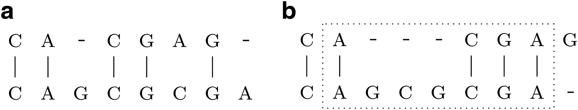
Examples of a sequence alignment and a regular language constrained sequence alignment. Sequence alignment and a regular language constrained sequence alignment on the two strings CACGAG and CAGCGCGA, with a scoring matrix (−1 for mismatch/insert/delete, 1 for match). (a) The maximal score of the global alignment is 2. (b) Let R be A(G + C)*GA, the constrained problem's score is 1.

1.1. Our contribution

In this article, we further speed up the algorithms for Regular Language Constrained Sequence Alignment by reducing their worst case time complexity bound to O(n²t³/ log t). This is done by establishing an optimal bound on the size of Straight-Line Programs (SLP) solving the maxima computation subproblem of the basic dynamic programming algorithm. We also study another solution based on a Steiner Tree computation. While it does not improve the worst case, our simulations show that both approaches are efficient in practice, especially when the input automata are dense.

Roadmap: The rest of this article proceeds as follows: In this section, we define the Regular Language Constrained Sequence Alignment Problem and give an overview of previous algorithms for the problem. In Section 2, we describe and analyze two new algorithms based on Steiner Trees and SLPs. Experimental results appear in Section 3.

1.2. Preliminaries and definitions

Let Σ be a finite alphabet. Let \documentclass{aastex}\usepackage{amsbsy}\usepackage{amsfonts}\usepackage{amssymb}\usepackage{bm}\usepackage{mathrsfs}\usepackage{pifont}\usepackage{stmaryrd}\usepackage{textcomp}\usepackage{portland,xspace}\usepackage{amsmath,amsxtra}\pagestyle{empty}\DeclareMathSizes{10}{9}{7}{6} \begin{document} $$a, b \in \Sigma^*$$ \end{document} two strings over the alphabet Σ. We denote a_i_,j the substring of a from index i to index j (inclusive) and a_i denotes the i^th letter in a. Let Σ′ = Σ ∪ { − } be an extended alphabet, where \documentclass{aastex}\usepackage{amsbsy}\usepackage{amsfonts}\usepackage{amssymb}\usepackage{bm}\usepackage{mathrsfs}\usepackage{pifont}\usepackage{stmaryrd}\usepackage{textcomp}\usepackage{portland,xspace}\usepackage{amsmath,amsxtra}\pagestyle{empty}\DeclareMathSizes{10}{9}{7}{6} \begin{document} $$- \notin \Sigma$$ \end{document} . Let \documentclass{aastex}\usepackage{amsbsy}\usepackage{amsfonts}\usepackage{amssymb}\usepackage{bm}\usepackage{mathrsfs}\usepackage{pifont}\usepackage{stmaryrd}\usepackage{textcomp}\usepackage{portland,xspace}\usepackage{amsmath,amsxtra}\pagestyle{empty}\DeclareMathSizes{10}{9}{7}{6} \begin{document} $$X, Y \in \Sigma^{ \prime *}$$ \end{document} . We denote X⁻, the string result of the removal of − letters from X. Let \documentclass{aastex}\usepackage{amsbsy}\usepackage{amsfonts}\usepackage{amssymb}\usepackage{bm}\usepackage{mathrsfs}\usepackage{pifont}\usepackage{stmaryrd}\usepackage{textcomp}\usepackage{portland,xspace}\usepackage{amsmath,amsxtra}\pagestyle{empty}\DeclareMathSizes{10}{9}{7}{6} \begin{document} $$s: \Sigma^{\prime} \times \Sigma^{ \prime} \setminus \{ -, - \} \rightarrow \Re^ +$$ \end{document} be a scoring function over edit operations (i.e., replace, insert, and delete). (X, Y) is an alignment of a and b if |X| = |Y|, X⁻ = a and Y⁻ = b. The score of an alignment (X, Y) is \documentclass{aastex}\usepackage{amsbsy}\usepackage{amsfonts}\usepackage{amssymb}\usepackage{bm}\usepackage{mathrsfs}\usepackage{pifont}\usepackage{stmaryrd}\usepackage{textcomp}\usepackage{portland,xspace}\usepackage{amsmath,amsxtra}\pagestyle{empty}\DeclareMathSizes{10}{9}{7}{6} \begin{document} $$s ((X, Y)) = \sum \limits_{i = 1}^{ \mid X \mid }s (X_i, Y_i)$$ \end{document} .

Let L_R be a regular language and let A = (Q, Σ, δ, q₀, F_A) be an NFA with t states, such that L(A) = L_R. We use a fixed numbering of the states in Q, \documentclass{aastex}\usepackage{amsbsy}\usepackage{amsfonts}\usepackage{amssymb}\usepackage{bm}\usepackage{mathrsfs}\usepackage{pifont}\usepackage{stmaryrd}\usepackage{textcomp}\usepackage{portland,xspace}\usepackage{amsmath,amsxtra}\pagestyle{empty}\DeclareMathSizes{10}{9}{7}{6} \begin{document} $$q_0, q_1, \ldots, q_{t - 1}$$ \end{document} . We assume, without loss of generality, that ε-transitions were removed from A and that the empty word ε is not in L(A).We denote the number of transitions in δ as |δ|. We use two notations for transitions, as follows. First, we denote by \documentclass{aastex}\usepackage{amsbsy}\usepackage{amsfonts}\usepackage{amssymb}\usepackage{bm}\usepackage{mathrsfs}\usepackage{pifont}\usepackage{stmaryrd}\usepackage{textcomp}\usepackage{portland,xspace}\usepackage{amsmath,amsxtra}\pagestyle{empty}\DeclareMathSizes{10}{9}{7}{6} \begin{document} $$q{ \mathop{ \rightarrow} \limits^{c}}p$$ \end{document} a transition in δ from state q to state p by letter c. Second, we add a notation for sets of transitions with a specific letter (Fig. 2a). Let pred_c(q) be the set of states with outgoing transitions labeled by letter c and leading to state q. \documentclass{aastex}\usepackage{amsbsy}\usepackage{amsfonts}\usepackage{amssymb}\usepackage{bm}\usepackage{mathrsfs}\usepackage{pifont}\usepackage{stmaryrd}\usepackage{textcomp}\usepackage{portland,xspace}\usepackage{amsmath,amsxtra}\pagestyle{empty}\DeclareMathSizes{10}{9}{7}{6} \begin{document} \begin{align*} pred_c (q) = \{ p \mid p{ \mathop{ \rightarrow} \limits^{c}}q \} \tag{1} \end{align*} \end{document}

Definition 1

(Regular Language Constrained Sequence Alignment). Given two strings a and b, over a fixed alphabet Σ, a scoring function s and an NFA A. Find an alignment (X, Y) of a and b such that it is the alignment with the maximal score under s which satisfies the following condition: indices i and j exist such that \documentclass{aastex}\usepackage{amsbsy}\usepackage{amsfonts}\usepackage{amssymb}\usepackage{bm}\usepackage{mathrsfs}\usepackage{pifont}\usepackage{stmaryrd}\usepackage{textcomp}\usepackage{portland,xspace}\usepackage{amsmath,amsxtra}\pagestyle{empty}\DeclareMathSizes{10}{9}{7}{6} \begin{document} $$X_{i, j}^ -, Y_{i, j}^ - \in L (A)$$ \end{document} .

1.3. An overview of previous work

Arslan's algorithm defines an NFA M, such that the states of M are the ordered pairs of states of A, therefore, it has O(t²) reachable states. M is defined over the alphabet Σ′ × Σ′. For every two transitions \documentclass{aastex}\usepackage{amsbsy}\usepackage{amsfonts}\usepackage{amssymb}\usepackage{bm}\usepackage{mathrsfs}\usepackage{pifont}\usepackage{stmaryrd}\usepackage{textcomp}\usepackage{portland,xspace}\usepackage{amsmath,amsxtra}\pagestyle{empty}\DeclareMathSizes{10}{9}{7}{6} \begin{document} $$q_1{ \mathop{ \rightarrow} \limits^{c_1}}p_1$$ \end{document} and \documentclass{aastex}\usepackage{amsbsy}\usepackage{amsfonts}\usepackage{amssymb}\usepackage{bm}\usepackage{mathrsfs}\usepackage{pifont}\usepackage{stmaryrd}\usepackage{textcomp}\usepackage{portland,xspace}\usepackage{amsmath,amsxtra}\pagestyle{empty}\DeclareMathSizes{10}{9}{7}{6} \begin{document} $$q_2{ \mathop{ \rightarrow} \limits^{c_2}}p_2$$ \end{document} in A, the transitions \documentclass{aastex}\usepackage{amsbsy}\usepackage{amsfonts}\usepackage{amssymb}\usepackage{bm}\usepackage{mathrsfs}\usepackage{pifont}\usepackage{stmaryrd}\usepackage{textcomp}\usepackage{portland,xspace}\usepackage{amsmath,amsxtra}\pagestyle{empty}\DeclareMathSizes{10}{9}{7}{6} \begin{document} $$(q_1, q_2) { \mathop{ \longrightarrow} \limits^{ (c_1, c_2) }} (p_1, p_2)$$ \end{document} , \documentclass{aastex}\usepackage{amsbsy}\usepackage{amsfonts}\usepackage{amssymb}\usepackage{bm}\usepackage{mathrsfs}\usepackage{pifont}\usepackage{stmaryrd}\usepackage{textcomp}\usepackage{portland,xspace}\usepackage{amsmath,amsxtra}\pagestyle{empty}\DeclareMathSizes{10}{9}{7}{6} \begin{document} $$(q_1, q_2) { \mathop{ \longrightarrow} \limits^{ (c_1, -) }} (p_1, q_2)$$ \end{document} and \documentclass{aastex}\usepackage{amsbsy}\usepackage{amsfonts}\usepackage{amssymb}\usepackage{bm}\usepackage{mathrsfs}\usepackage{pifont}\usepackage{stmaryrd}\usepackage{textcomp}\usepackage{portland,xspace}\usepackage{amsmath,amsxtra}\pagestyle{empty}\DeclareMathSizes{10}{9}{7}{6} \begin{document} $$(q_1, q_2) { \mathop{ \longrightarrow} \limits^{ (-, c_2) }} (q_1, p_2)$$ \end{document} exist in M. For any two final (accepting) states \documentclass{aastex}\usepackage{amsbsy}\usepackage{amsfonts}\usepackage{amssymb}\usepackage{bm}\usepackage{mathrsfs}\usepackage{pifont}\usepackage{stmaryrd}\usepackage{textcomp}\usepackage{portland,xspace}\usepackage{amsmath,amsxtra}\pagestyle{empty}\DeclareMathSizes{10}{9}{7}{6} \begin{document} $$q_{f_1}, q_{f_2} \in F_A$$ \end{document} and for any letters c₁, c₂ the transitions \documentclass{aastex}\usepackage{amsbsy}\usepackage{amsfonts}\usepackage{amssymb}\usepackage{bm}\usepackage{mathrsfs}\usepackage{pifont}\usepackage{stmaryrd}\usepackage{textcomp}\usepackage{portland,xspace}\usepackage{amsmath,amsxtra}\pagestyle{empty}\DeclareMathSizes{10}{9}{7}{6} \begin{document} $$(q_{f_1}, q_{f_2}) { \mathop{ \longrightarrow} \limits^{ (c_1, c_2) }} (q_{f_1}, q_{f_2})$$ \end{document} , \documentclass{aastex}\usepackage{amsbsy}\usepackage{amsfonts}\usepackage{amssymb}\usepackage{bm}\usepackage{mathrsfs}\usepackage{pifont}\usepackage{stmaryrd}\usepackage{textcomp}\usepackage{portland,xspace}\usepackage{amsmath,amsxtra}\pagestyle{empty}\DeclareMathSizes{10}{9}{7}{6} \begin{document} $$(q_{f_1}, q_{f_2}) { \mathop{ \longrightarrow} \limits^{ (c_1, -) }} (q_{f_1}, q_{f_2})$$ \end{document} and \documentclass{aastex}\usepackage{amsbsy}\usepackage{amsfonts}\usepackage{amssymb}\usepackage{bm}\usepackage{mathrsfs}\usepackage{pifont}\usepackage{stmaryrd}\usepackage{textcomp}\usepackage{portland,xspace}\usepackage{amsmath,amsxtra}\pagestyle{empty}\DeclareMathSizes{10}{9}{7}{6} \begin{document} $$(q_{f_1}, q_{f_2}) { \mathop{ \longrightarrow} \limits^{ (-, c_2) }} (q_{f_1}, q_{f_2})$$ \end{document} exist in M. The same addition is done for the initial state. A sequence alignment table T of size (|a| + 1) × (|b| + 1) is calculated. Each cell, T_i,j contains a table of scores, one for every state in M (that is, a pair of states in A). T_i,j(p, q) is the maximal score of an alignment of a_1,i and b_1,j, such that reading it in M ends at (p, q). The table size is clearly O(n²t²), since each cell holds t² scores.

In the following recurrence formula for T_i_,j, we move from the notion of the alignment automaton M in Arslan to a simpler formulation. As a first step, we add to A transitions \documentclass{aastex}\usepackage{amsbsy}\usepackage{amsfonts}\usepackage{amssymb}\usepackage{bm}\usepackage{mathrsfs}\usepackage{pifont}\usepackage{stmaryrd}\usepackage{textcomp}\usepackage{portland,xspace}\usepackage{amsmath,amsxtra}\pagestyle{empty}\DeclareMathSizes{10}{9}{7}{6} \begin{document} $$q{ \mathop{ \rightarrow} \limits^{c}}q$$ \end{document} where c is any letter and q is either an initial or final state in A. The score of T_i_,j for a given state (p, q) is computed as follows. \documentclass{aastex}\usepackage{amsbsy}\usepackage{amsfonts}\usepackage{amssymb}\usepackage{bm}\usepackage{mathrsfs}\usepackage{pifont}\usepackage{stmaryrd}\usepackage{textcomp}\usepackage{portland,xspace}\usepackage{amsmath,amsxtra}\pagestyle{empty}\DeclareMathSizes{10}{9}{7}{6} \begin{document} \begin{align*} T_{i, j} (q, p) = \max \begin{cases} \max \{ T_{i - 1, j} ( q^{ \prime}, p) \mid q^{ \prime} \in pred_{a_i} (q) \} + s ( a_i, -), \\ \max \{ T_{i, j - 1} (q, p^{ \prime}) \mid p^{ \prime} \in pred_{b_j} (p) \} + s (-, b_j), \\ \max \{ T_{i - 1, j - 1} (q^{ \prime}, p^{ \prime}) \mid \\ \qquad \qquad q^{ \prime} \in pred_{a_i} (q), p^{ \prime} \in pred_{b_j} (p) \} + s (a_i, b_j) (*) \end{cases} \tag{2} \end{align*} \end{document}

The initialization consists of assigning 0 to T_0,0(q₀, q₀) and − ∞ elsewhere. We define max ∅ = − ∞. The optimal alignment score is \documentclass{aastex}\usepackage{amsbsy}\usepackage{amsfonts}\usepackage{amssymb}\usepackage{bm}\usepackage{mathrsfs}\usepackage{pifont}\usepackage{stmaryrd}\usepackage{textcomp}\usepackage{portland,xspace}\usepackage{amsmath,amsxtra}\pagestyle{empty}\DeclareMathSizes{10}{9}{7}{6} \begin{document} $$\max \{ T_{ \mid a \mid, \mid b \mid } (q, p) \mid q, p \in F_A \} $$ \end{document} . There are a total of O(n²t²) scores to calculate. According to Eq. 2, each score calculation (for a given i, j, q and p) involves O(t²) values, as apparent in the third term marked (*), because in an NFA there are at most t transitions \documentclass{aastex}\usepackage{amsbsy}\usepackage{amsfonts}\usepackage{amssymb}\usepackage{bm}\usepackage{mathrsfs}\usepackage{pifont}\usepackage{stmaryrd}\usepackage{textcomp}\usepackage{portland,xspace}\usepackage{amsmath,amsxtra}\pagestyle{empty}\DeclareMathSizes{10}{9}{7}{6} \begin{document} $$q^{ \prime}{ \mathop{ \rightarrow} \limits^{a_i}}q$$ \end{document} for a single letter a_i and, independently, there are at most t transitions \documentclass{aastex}\usepackage{amsbsy}\usepackage{amsfonts}\usepackage{amssymb}\usepackage{bm}\usepackage{mathrsfs}\usepackage{pifont}\usepackage{stmaryrd}\usepackage{textcomp}\usepackage{portland,xspace}\usepackage{amsmath,amsxtra}\pagestyle{empty}\DeclareMathSizes{10}{9}{7}{6} \begin{document} $$p^{ \prime}{ \mathop{ \rightarrow} \limits^{b_j}}q$$ \end{document} for b_j (Fig. 2b). The term (*) is the bottleneck of the algorithm. Since A is non-deterministic, it may contain O(t²) transitions by any letter c.

FIG. 2.

(a) An example of an NFA. Its transitions yield the following pred sets: \documentclass{aastex}\usepackage{amsbsy}\usepackage{amsfonts}\usepackage{amssymb}\usepackage{bm}\usepackage{mathrsfs}\usepackage{pifont}\usepackage{stmaryrd}\usepackage{textcomp}\usepackage{portland,xspace}\usepackage{amsmath,amsxtra}\pagestyle{empty}\DeclareMathSizes{10}{9}{7}{6} \begin{document} $$pred_A (q_0) = \emptyset$$ \end{document} , \documentclass{aastex}\usepackage{amsbsy}\usepackage{amsfonts}\usepackage{amssymb}\usepackage{bm}\usepackage{mathrsfs}\usepackage{pifont}\usepackage{stmaryrd}\usepackage{textcomp}\usepackage{portland,xspace}\usepackage{amsmath,amsxtra}\pagestyle{empty}\DeclareMathSizes{10}{9}{7}{6} \begin{document} $$pred_A (q_1) =\{ q_0, q_1, q_2 \} $$ \end{document} , \documentclass{aastex}\usepackage{amsbsy}\usepackage{amsfonts}\usepackage{amssymb}\usepackage{bm}\usepackage{mathrsfs}\usepackage{pifont}\usepackage{stmaryrd}\usepackage{textcomp}\usepackage{portland,xspace}\usepackage{amsmath,amsxtra}\pagestyle{empty}\DeclareMathSizes{10}{9}{7}{6} \begin{document} $$pred_A (q_2) =pred_C (q_1) =\{ q_0 \} $$ \end{document} , \documentclass{aastex}\usepackage{amsbsy}\usepackage{amsfonts}\usepackage{amssymb}\usepackage{bm}\usepackage{mathrsfs}\usepackage{pifont}\usepackage{stmaryrd}\usepackage{textcomp}\usepackage{portland,xspace}\usepackage{amsmath,amsxtra}\pagestyle{empty}\DeclareMathSizes{10}{9}{7}{6} \begin{document} $$pred_C (q_0) = \{ q_2 \} $$ \end{document} , \documentclass{aastex}\usepackage{amsbsy}\usepackage{amsfonts}\usepackage{amssymb}\usepackage{bm}\usepackage{mathrsfs}\usepackage{pifont}\usepackage{stmaryrd}\usepackage{textcomp}\usepackage{portland,xspace}\usepackage{amsmath,amsxtra}\pagestyle{empty}\DeclareMathSizes{10}{9}{7}{6} \begin{document} $$pred_C (q_2) = \{ q_0, q_2 \} $$ \end{document} . (b) Score calculations performed by Arslan's algorithm. The green scores in T_i_−1,j−1, corresponding to rows \documentclass{aastex}\usepackage{amsbsy}\usepackage{amsfonts}\usepackage{amssymb}\usepackage{bm}\usepackage{mathrsfs}\usepackage{pifont}\usepackage{stmaryrd}\usepackage{textcomp}\usepackage{portland,xspace}\usepackage{amsmath,amsxtra}\pagestyle{empty}\DeclareMathSizes{10}{9}{7}{6} \begin{document} $$pred_{a_i} (q)$$ \end{document} and columns \documentclass{aastex}\usepackage{amsbsy}\usepackage{amsfonts}\usepackage{amssymb}\usepackage{bm}\usepackage{mathrsfs}\usepackage{pifont}\usepackage{stmaryrd}\usepackage{textcomp}\usepackage{portland,xspace}\usepackage{amsmath,amsxtra}\pagestyle{empty}\DeclareMathSizes{10}{9}{7}{6} \begin{document} $$pred_{b_j} (p)$$ \end{document} , are used in the calculation of T_i,_,j for the state pair (q, p).

The algorithm of Chung et al. (2007b) exploits the following redundancy: Given that M is an NFA with |δ| = O(t²) states, and assuming no additional knowledge of M, it can be concluded that M can potentially have O(t⁴) transitions. Thus, Arslan's algorithm iterates over all possibilities of two states of M in each T_i_,j calculation. However, it is known, according to the way M was built, that each transition in M originates from at most two transitions in A. The iteration over the two possible transitions can be done independently of each other.

Chung et al. (2007b) improved the time complexity of Arslan's algorithm by removing redundant computations which were due to the fact that the computed value is based on two independent optimum calculations, one for each of the compared strings. We next describe Chung et al.'s algorithm using our own notation, in Eq. 3 and Eq. 4. The calculation of (*) is split into two steps using an intermediate table L (Fig. 3). \documentclass{aastex}\usepackage{amsbsy}\usepackage{amsfonts}\usepackage{amssymb}\usepackage{bm}\usepackage{mathrsfs}\usepackage{pifont}\usepackage{stmaryrd}\usepackage{textcomp}\usepackage{portland,xspace}\usepackage{amsmath,amsxtra}\pagestyle{empty}\DeclareMathSizes{10}{9}{7}{6} \begin{document} \begin{align*} L_{i, j} (q, p^{ \prime}) = \max \{ T_{i - 1, j - 1} (q^{ \prime}, p^{ \prime}) \mid q^{ \prime} \in pred_{a_i} (q) \} \tag{3} \end{align*} \end{document} \documentclass{aastex}\usepackage{amsbsy}\usepackage{amsfonts}\usepackage{amssymb}\usepackage{bm}\usepackage{mathrsfs}\usepackage{pifont}\usepackage{stmaryrd}\usepackage{textcomp}\usepackage{portland,xspace}\usepackage{amsmath,amsxtra}\pagestyle{empty}\DeclareMathSizes{10}{9}{7}{6} \begin{document} \begin{align*} T_{i, j} (q, p) = \max \{ L_{i, j} (q, p^{ \prime}) \mid p^{ \prime} \in pred_{b_j} (p) \} + s (a_i, b_j)\tag{4} \end{align*} \end{document}

In the first step (Eq. 3), the size of the set, over which the maximum is calculated for every pair of states (q, p′), depends on the existing transitions with the letter a_i. Since the size of the set is bounded (i.e., |pred_ai(q)| ≤ t), this step takes O(t³) time. The same argument holds for the second step (Eq. 4). In summary, their algorithm improved the time complexity to O(n²t|δ|) = O(n²t³), while maintaining the same space complexity.

2. A Faster Algorithm

2.1. Eliminating duplicate computations

It is apparent from Eq. (3) and Eq. (4) that the calculation of L_i_,j, for a specific value of p′ and ranging over q, computes the maximum for subsets of indices of column p′ of T_i_−1,j−1, while the calculation of T_i_,j, for a specific value of q and ranging over p, computes the maximum for subsets of indices of the q^th row of L_i_,j (Fig. 3). The structure of the NFA transition table, namely the relations between the pred_c sets, can be used to reduce the number of components required in consecutive subset maxima calculations. For instance, let us assume that a state q′ is included both in pred_c(q₁) and pred_c(q₂) for q₁ ≠ q₂. Then, for a given state p, the score T_i_−1,j−1(q′, p) is taken into account in calculations of both L_i_,j(q₁, p) and L_i_,j(q₂, p) (Fig. 4). By minimizing the repetition of score usage, the efficiency of the calculation of Eq. (3) and Eq. (4) can be improved.

FIG. 3.

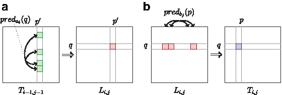
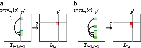
Score calculation performed by Chung et al.'s algorithm. (a) Calculation of L_i,_,j. (b) Calculation of T_i,_,j.

FIG. 4.

Similar and duplicate score calculations in Chung et al.'s algorithm can be reused. (a) The calculation of a single score in L_i,_,j depends on several scores in T_i_−1,j−1. (b) The calculation of another score in L_i,_,j (in this example, for row q + 1) can be done according to the previously calculated score of q and some additional scores from T_i_−1,j−1, marked in bold.

Following this observation, the goal of speeding up the calculation of Eq. (3) and Eq. (4) can be formulated as a question: What is the most efficient way to calculate maximum values over given, possibly overlapping, sets of scores? Thus, the general subproblem underlying the speed up of these algorithms can be formulated as follows.

Definition 2

(Subsets Maxima Problem). Let W be a set of scores, with |W| = t and let \documentclass{aastex}\usepackage{amsbsy}\usepackage{amsfonts}\usepackage{amssymb}\usepackage{bm}\usepackage{mathrsfs}\usepackage{pifont}\usepackage{stmaryrd}\usepackage{textcomp}\usepackage{portland,xspace}\usepackage{amsmath,amsxtra}\pagestyle{empty}\DeclareMathSizes{10}{9}{7}{6} \begin{document} $$V = \langle v_0, \ldots, v_{t - 1} \rangle$$ \end{document} be t subsets of W (v_k ⊆ W). Calculate max v_k for each \documentclass{aastex}\usepackage{amsbsy}\usepackage{amsfonts}\usepackage{amssymb}\usepackage{bm}\usepackage{mathrsfs}\usepackage{pifont}\usepackage{stmaryrd}\usepackage{textcomp}\usepackage{portland,xspace}\usepackage{amsmath,amsxtra}\pagestyle{empty}\DeclareMathSizes{10}{9}{7}{6} \begin{document} $$v_k \in V$$ \end{document} .

For Eq. 3, having fixed values of i, j and p′, the set of scores W consists of t scores in T_i_{−1, j−1} and V consists of scores which correspond to all possible \documentclass{aastex}\usepackage{amsbsy}\usepackage{amsfonts}\usepackage{amssymb}\usepackage{bm}\usepackage{mathrsfs}\usepackage{pifont}\usepackage{stmaryrd}\usepackage{textcomp}\usepackage{portland,xspace}\usepackage{amsmath,amsxtra}\pagestyle{empty}\DeclareMathSizes{10}{9}{7}{6} \begin{document} $$pred_{a_{i}}$$ \end{document} subsets. More formally: \documentclass{aastex}\usepackage{amsbsy}\usepackage{amsfonts}\usepackage{amssymb}\usepackage{bm}\usepackage{mathrsfs}\usepackage{pifont}\usepackage{stmaryrd}\usepackage{textcomp}\usepackage{portland,xspace}\usepackage{amsmath,amsxtra}\pagestyle{empty}\DeclareMathSizes{10}{9}{7}{6} \begin{document} \begin{align*} W &= \{ T_{i - 1, j - 1} (q^{ \prime}, p^{ \prime}) \mid q^{ \prime} \in Q \} \\ V &= \langle v_0, \ldots, v_{t - 1} \rangle, v_k = \{ T_{i - 1 , j - 1} (q^{ \prime}, p^{ \prime}) \mid q^{ \prime} \in pred_{a_i} (q_k) \} \tag{5} \end{align*} \end{document}

The values of W and V are similarly established for Eq. 4.

We represent each subset v_k in V by a Boolean vector, where the l^th bit reflects the membership of the l^th score in the subset \documentclass{aastex}\usepackage{amsbsy}\usepackage{amsfonts}\usepackage{amssymb}\usepackage{bm}\usepackage{mathrsfs}\usepackage{pifont}\usepackage{stmaryrd}\usepackage{textcomp}\usepackage{portland,xspace}\usepackage{amsmath,amsxtra}\pagestyle{empty}\DeclareMathSizes{10}{9}{7}{6} \begin{document} $$pred_{a_{i}}$$ \end{document} (q_k). Thus, V is represented by a tuple of Boolean vectors, denoted S. In the following sections, we discuss two alternative ways of solving the Subsets Maxima Problem: one based on Steiner trees (Section 2.2) and the other based on SLPs (Section 2.3).

2.2. An algorithm based on a Steiner minimal directed tree

In this section, we explore the possibility of employing Steiner minimal directed trees to solve the Subsets Maxima Problem. We show that the size of a Steiner minimal directed tree for a tuple of Boolean vectors S, as described above, is not greater than the number of transitions of the NFA. Thus, using a heuristic algorithm for Steiner minimal directed trees improves the run-time of our solution to Regular Language Constrained Alignment in practice, as demonstrated by our simulations (see Section 3). But first, we give a formal definition of Steiner minimal directed trees and review related work.

There are several Steiner tree problems studied in the literature. The general Steiner tree problem is the problem of spanning a subset of vertices of a (directed or undirected) graph, while including a minimal number of additional nodes. The problem is NP-hard (Bern and Plassmann, 1989; Shi and Su, 2006). Here, we are interested in the Steiner minimal directed tree problem in a specific graph, namely the Hamming hypercube. In the Hamming hypercube, the Hamming distance between any two adjacent nodes of the tree, v and u, is 1. That is, either u has exactly one 1-valued bit which is 0-valued in v or vice versa. This version of the Steiner minimal tree problem is also NP-hard (Foulds and Graham, 1982). There are several heuristic solutions for these problems (Jia et al., 2004; Lin and Ni, 1993; Sheu and Yang, 2001).

Definition 3

(The Steiner Minimal Directed Tree Problem for Hamming Hypercubes). Given a set S of k d-dimensional points, find a rooted tree in the H^d Hamming hypercube that spans S, has the minimal possible size N and all edges are directed away from the root (For all v and u such that v is the parent of u in the tree, u has exactly one 1-valued bit which is 0-valued in v.)

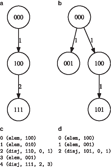
Given a Steiner minimal directed tree for a tuple of Boolean vectors, S, the subsets maxima of the corresponding weight-subsets tuple, V, can be calculated by traversing the tree in a top-down fashion. The reader is referred to Figure 5a,b for an example of the construction of Steiner trees for a specific NFA.

FIG. 5.

(a) An example of Steiner tree construction for pred_A. (b) An example of Steiner tree construction for pred_C. (c) An example of Four Russians based SLP construction for pred_A. (d) An example for Four Russians based SLP construction for pred_C.

Theorem 1

(upper bound of |δ| for the size of the Steiner Minimal Directed Tree). Let A = (Q, Σ, δ, q₀, F_A) be an NFA and let S_c, for \documentclass{aastex}\usepackage{amsbsy}\usepackage{amsfonts}\usepackage{amssymb}\usepackage{bm}\usepackage{mathrsfs}\usepackage{pifont}\usepackage{stmaryrd}\usepackage{textcomp}\usepackage{portland,xspace}\usepackage{amsmath,amsxtra}\pagestyle{empty}\DeclareMathSizes{10}{9}{7}{6} \begin{document} $$c \in \Sigma$$ \end{document} , be sets of Boolean vectors corresponding to δ, as described in Subsection 2.1. There exist Steiner directed trees for sets S_c, such that the sum of their sizes is not greater than |δ| + t.

Proof. S_c, for a specific c, is a set of Boolean vectors representing pred_c(A). Thus, the total number of 1-valued bits in all S_c sets equals |δ|. For each set S_c, we build a Steiner directed tree, as follows. Let X be a Boolean vector in S_c, such that bits \documentclass{aastex}\usepackage{amsbsy}\usepackage{amsfonts}\usepackage{amssymb}\usepackage{bm}\usepackage{mathrsfs}\usepackage{pifont}\usepackage{stmaryrd}\usepackage{textcomp}\usepackage{portland,xspace}\usepackage{amsmath,amsxtra}\pagestyle{empty}\DeclareMathSizes{10}{9}{7}{6} \begin{document} $$x_1, x_2 \ldots, x_k$$ \end{document} in X are 1-valued (i.e., X has k 1's). Starting from the zero vector, 0^t, as the root, we add a chain of nodes in the Steiner tree until X is reached. The first node connected to 0^t is the elementary vector with the x₁ bit 1-valued. Similarly, the i^th node is a vector that has all bits equal to its parent node, except for the x_i bit, which is 1-valued in that vector, but 0-valued in the parent vector. This path reaches vector X by adding at most k nodes (not including the zero vector). The total length of the tree S_c is not greater than the total number of 1-valued bits in S_c plus 1 (for the zero vector). Thus, such Steiner directed trees, for sets S_c, have the sum of their lengths not greater that |δ| + t. ■

Theorem 2

(lower bound). The size of the minimal Steiner tree for a set S of size t is N = Ω(t²).

Proof. For every natural t, we show the existence of a t-sized set S such that N is in the order of t². Let us assume that t = 2^k for a natural number k. We select S to be any t Boolean vectors from the k-dimensional Hadamard code (Dinur and Safra, 2005; Sylvester, 1867; Seberry and Yamada, 1992). The Hadamard code contains 2t = 2^k+1 vectors, each of length t = 2^k, such that each two vectors have a Hamming distance of at least \documentclass{aastex}\usepackage{amsbsy}\usepackage{amsfonts}\usepackage{amssymb}\usepackage{bm}\usepackage{mathrsfs}\usepackage{pifont}\usepackage{stmaryrd}\usepackage{textcomp}\usepackage{portland,xspace}\usepackage{amsmath,amsxtra}\pagestyle{empty}\DeclareMathSizes{10}{9}{7}{6} \begin{document} $$ { t } / { 2 } = 2^ { k - 1 } $$ \end{document} . The Hamming distance within S is at least \documentclass{aastex}\usepackage{amsbsy}\usepackage{amsfonts}\usepackage{amssymb}\usepackage{bm}\usepackage{mathrsfs}\usepackage{pifont}\usepackage{stmaryrd}\usepackage{textcomp}\usepackage{portland,xspace}\usepackage{amsmath,amsxtra}\pagestyle{empty}\DeclareMathSizes{10}{9}{7}{6} \begin{document} $$ { t }/ { 2 } $$ \end{document} (the ( \documentclass{aastex}\usepackage{amsbsy}\usepackage{amsfonts}\usepackage{amssymb}\usepackage{bm}\usepackage{mathrsfs}\usepackage{pifont}\usepackage{stmaryrd}\usepackage{textcomp}\usepackage{portland,xspace}\usepackage{amsmath,amsxtra}\pagestyle{empty}\DeclareMathSizes{10}{9}{7}{6} \begin{document} $$ { t }/ { 4 } - 1$$ \end{document} )-radius ball surrounding each vector in S does not contain any other vector in S). Moreover, \documentclass{aastex}\usepackage{amsbsy}\usepackage{amsfonts}\usepackage{amssymb}\usepackage{bm}\usepackage{mathrsfs}\usepackage{pifont}\usepackage{stmaryrd}\usepackage{textcomp}\usepackage{portland,xspace}\usepackage{amsmath,amsxtra}\pagestyle{empty}\DeclareMathSizes{10}{9}{7}{6} \begin{document} $$ { t } /{ 4 } - 1$$ \end{document} -radius balls, surrounding different vectors in S, are disjoint. Thus, a tree that spans S requires at least \documentclass{aastex}\usepackage{amsbsy}\usepackage{amsfonts}\usepackage{amssymb}\usepackage{bm}\usepackage{mathrsfs}\usepackage{pifont}\usepackage{stmaryrd}\usepackage{textcomp}\usepackage{portland,xspace}\usepackage{amsmath,amsxtra}\pagestyle{empty}\DeclareMathSizes{10}{9}{7}{6} \begin{document} $$t ({ t }/ { 4 } - 1)$$ \end{document} Steiner nodes. ■

From theorems 1 and 2, it follows that the size of the Steiner minimal tree is N = Θ(t²) in the worst case. Thus, our Steiner-based algorithm, in the framework of Chung et al., runs in O(n²t³) time. In Section 3, we compare the sizes of heuristic Steiner directed trees with the sizes of the corresponding transition tables for simulated NFAs. Our simulations show that, even though the Steiner-based algorithm does not yield the theoretical bounds obtained for SLPs, in practice it performs very well.

2.3. A solution to subsets maxima via SLPs

We start by introducing the notion of a Straight-Line Program with Boolean operations.

Definition 4

(SLP with Boolean operations). We are given a tuple of t Boolean vectors \documentclass{aastex}\usepackage{amsbsy}\usepackage{amsfonts}\usepackage{amssymb}\usepackage{bm}\usepackage{mathrsfs}\usepackage{pifont}\usepackage{stmaryrd}\usepackage{textcomp}\usepackage{portland,xspace}\usepackage{amsmath,amsxtra}\pagestyle{empty}\DeclareMathSizes{10}{9}{7}{6} \begin{document} $$S = \langle x_1, \ldots, x_t \rangle$$ \end{document} , \documentclass{aastex}\usepackage{amsbsy}\usepackage{amsfonts}\usepackage{amssymb}\usepackage{bm}\usepackage{mathrsfs}\usepackage{pifont}\usepackage{stmaryrd}\usepackage{textcomp}\usepackage{portland,xspace}\usepackage{amsmath,amsxtra}\pagestyle{empty}\DeclareMathSizes{10}{9}{7}{6} \begin{document} $$x_i \in \{ 0, 1 \} ^m$$ \end{document} . An SLP is a sequence of instructions P, of two types:

\documentclass{aastex}\usepackage{amsbsy}\usepackage{amsfonts}\usepackage{amssymb}\usepackage{bm}\usepackage{mathrsfs}\usepackage{pifont}\usepackage{stmaryrd}\usepackage{textcomp}\usepackage{portland,xspace}\usepackage{amsmath,amsxtra}\pagestyle{empty}\DeclareMathSizes{10}{9}{7}{6} \begin{document} $$\beta_i : = (0, \ldots, 0, 1, 0, \ldots, 0)$$ \end{document} (elementary vector),

\documentclass{aastex}\usepackage{amsbsy}\usepackage{amsfonts}\usepackage{amssymb}\usepackage{bm}\usepackage{mathrsfs}\usepackage{pifont}\usepackage{stmaryrd}\usepackage{textcomp}\usepackage{portland,xspace}\usepackage{amsmath,amsxtra}\pagestyle{empty}\DeclareMathSizes{10}{9}{7}{6} \begin{document} $$\beta_i : = \beta_{j}\vee \beta_{l}$$ \end{document} , with j, l < i (disjunction).

An SLP computes the left-hand side vectors of its instructions \documentclass{aastex}\usepackage{amsbsy}\usepackage{amsfonts}\usepackage{amssymb}\usepackage{bm}\usepackage{mathrsfs}\usepackage{pifont}\usepackage{stmaryrd}\usepackage{textcomp}\usepackage{portland,xspace}\usepackage{amsmath,amsxtra}\pagestyle{empty}\DeclareMathSizes{10}{9}{7}{6} \begin{document} $$\langle \beta_1, \ldots, \beta_N \rangle$$ \end{document} , \documentclass{aastex}\usepackage{amsbsy}\usepackage{amsfonts}\usepackage{amssymb}\usepackage{bm}\usepackage{mathrsfs}\usepackage{pifont}\usepackage{stmaryrd}\usepackage{textcomp}\usepackage{portland,xspace}\usepackage{amsmath,amsxtra}\pagestyle{empty}\DeclareMathSizes{10}{9}{7}{6} \begin{document} $$\beta_i \in \{ 0, 1 \} ^m.$$ \end{document} An SLP P computes S if \documentclass{aastex}\usepackage{amsbsy}\usepackage{amsfonts}\usepackage{amssymb}\usepackage{bm}\usepackage{mathrsfs}\usepackage{pifont}\usepackage{stmaryrd}\usepackage{textcomp}\usepackage{portland,xspace}\usepackage{amsmath,amsxtra}\pagestyle{empty}\DeclareMathSizes{10}{9}{7}{6} \begin{document} $$\langle \beta_{N - t + 1}, \ldots, \beta_N \rangle = S$$ \end{document} .

The Subsets Maxima Problem can be reduced to the problem of finding the shortest possible SLP with Boolean operations. In order to use SLPs for the task of subsets maxima calculation, we represent V as a tuple of Boolean vectors, S, as described in Subsection 2.1. Given an SLP for S, the subsets maxima can be calculated by following the SLP in linear order: if β_h is an elementary vector, having the i^th bit equal to 1, the vector is assigned the value of the i^th score and if β_h is a binary disjunction of β_j and β_k, then it is assigned the value of the maximum of their assigned scores. If β_h represents a subset from V, its score is reported.

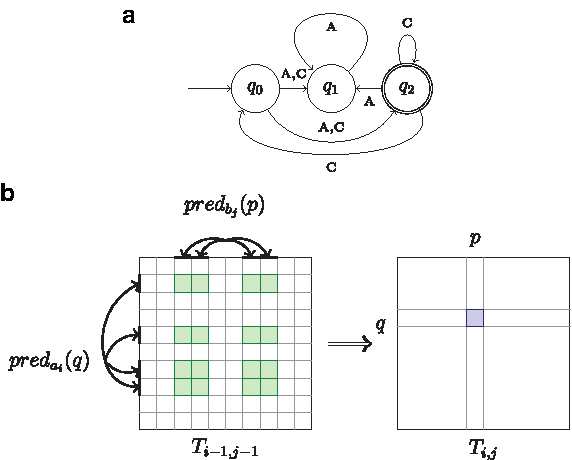
The reader is referred to Figure 5c,d for an example of the constructions of SLPs for a specific NFA. These constructions take as input the example NFA appearing in Figure 2a. SLP operation types “elementary vector” and “disjunction” are abbreviated.

For the purpose of utilizing SLPs for the Subsets Maxima Problem, in the rest of this section we address the following goal: given a tuple S of t Boolean vectors of length t, construct an SLP for S of minimal length. This goal is achieved via the following two theorems.

Theorem 3

(upper bound). An SLP for S can be generated such that: (1) \documentclass{aastex}\usepackage{amsbsy}\usepackage{amsfonts}\usepackage{amssymb}\usepackage{bm}\usepackage{mathrsfs}\usepackage{pifont}\usepackage{stmaryrd}\usepackage{textcomp}\usepackage{portland,xspace}\usepackage{amsmath,amsxtra}\pagestyle{empty}\DeclareMathSizes{10}{9}{7}{6} \begin{document} $$N \leq { 2t^2 }/ { \log t } $$ \end{document} , where N denotes the size of the SLP, and (2) the time required to construct it is \documentclass{aastex}\usepackage{amsbsy}\usepackage{amsfonts}\usepackage{amssymb}\usepackage{bm}\usepackage{mathrsfs}\usepackage{pifont}\usepackage{stmaryrd}\usepackage{textcomp}\usepackage{portland,xspace}\usepackage{amsmath,amsxtra}\pagestyle{empty}\DeclareMathSizes{10}{9}{7}{6} \begin{document} $$O ({ t^2 } / { \log t })$$ \end{document} .

Proof. We will use the Four-Russians technique. A similar argument is applied in Savage (1974).

Split each vector of S into b = t/ log t blocks of length log t. Each block has 2^{log t} = t possible values. For each i = 1.b, consider the set of all block vectors, denoted W_i, such that block i takes all possible values and the other blocks are all 0-valued bits. All vectors of W_i can be generated incrementally with t operations (in a bottom-up fashion): First all vectors in W_i which have a single 1-valued bit are generated, then all vectors in W_i which have two 1-valued bits are generated by the disjunction of two vectors in W_i with a single 1-valued bit. In general, all vectors in W_i which have j + 1 1-valued bits are generated by adding disjunction operations between vectors in W_i which have j 1-valued bits and vectors in W_i with one 1-valued bit. Therefore, there are a total of \documentclass{aastex}\usepackage{amsbsy}\usepackage{amsfonts}\usepackage{amssymb}\usepackage{bm}\usepackage{mathrsfs}\usepackage{pifont}\usepackage{stmaryrd}\usepackage{textcomp}\usepackage{portland,xspace}\usepackage{amsmath,amsxtra}\pagestyle{empty}\DeclareMathSizes{10}{9}{7}{6} \begin{document} $$bt = { t^2 }/ { \log t } $$ \end{document} block vectors and it takes \documentclass{aastex}\usepackage{amsbsy}\usepackage{amsfonts}\usepackage{amssymb}\usepackage{bm}\usepackage{mathrsfs}\usepackage{pifont}\usepackage{stmaryrd}\usepackage{textcomp}\usepackage{portland,xspace}\usepackage{amsmath,amsxtra}\pagestyle{empty}\DeclareMathSizes{10}{9}{7}{6} \begin{document} $$O ({ t^2 } /{ \log t })$$ \end{document} time to create all the block vectors.

Each vector of S can then be generated in b − 1 disjunction operations from pre-computed block vectors and there are t vectors in S. All the vectors of S are, therefore, computed by adding t(b − 1) ≤ t²/log t operations to the SLP.

The length of the underlying SLP constructed here, equals the number of disjunction and elementary operations, summed over both stages (block vector creation plus computing S from the block vectors), which is at most \documentclass{aastex}\usepackage{amsbsy}\usepackage{amsfonts}\usepackage{amssymb}\usepackage{bm}\usepackage{mathrsfs}\usepackage{pifont}\usepackage{stmaryrd}\usepackage{textcomp}\usepackage{portland,xspace}\usepackage{amsmath,amsxtra}\pagestyle{empty}\DeclareMathSizes{10}{9}{7}{6} \begin{document} $$ { 2t^2 } / { \log t } $$ \end{document} . The time required for the construction of the SLP is \documentclass{aastex}\usepackage{amsbsy}\usepackage{amsfonts}\usepackage{amssymb}\usepackage{bm}\usepackage{mathrsfs}\usepackage{pifont}\usepackage{stmaryrd}\usepackage{textcomp}\usepackage{portland,xspace}\usepackage{amsmath,amsxtra}\pagestyle{empty}\DeclareMathSizes{10}{9}{7}{6} \begin{document} $$O ({ t^2 } / { \log t })$$ \end{document} . ■

Remark. Note that the bound in Theorem 3 can be improved by a factor of two by taking blocks of size log t − log log t.

The above bound is very close to the information-theoretic lower bound, as shown below.

Theorem 4

(lower bound). An SLP for S requires \documentclass{aastex}\usepackage{amsbsy}\usepackage{amsfonts}\usepackage{amssymb}\usepackage{bm}\usepackage{mathrsfs}\usepackage{pifont}\usepackage{stmaryrd}\usepackage{textcomp}\usepackage{portland,xspace}\usepackage{amsmath,amsxtra}\pagestyle{empty}\DeclareMathSizes{10}{9}{7}{6} \begin{document} $$\Omega ({ t^2 } / { \log t })$$ \end{document} operations.

Proof. We use the standard counting argument. Again, a similar proof can be found in Savage (1974).

There are t distinct elementary vector type instructions and, in the minimal SLP, each of them occurs at most once. Without loss of generality, we assume that the initialization instructions form the t first instructions in the SLP in any fixed order.

Let q be the number of disjunction instructions, i.e., N = t + q. There are at most N² possibilities for each disjunction instruction and, therefore, there are at most (N²)^q = N^2q different SLPs of length N. On the other hand, there are (2^t)^t = 2^t2 different tuples S. We then should have \documentclass{aastex}\usepackage{amsbsy}\usepackage{amsfonts}\usepackage{amssymb}\usepackage{bm}\usepackage{mathrsfs}\usepackage{pifont}\usepackage{stmaryrd}\usepackage{textcomp}\usepackage{portland,xspace}\usepackage{amsmath,amsxtra}\pagestyle{empty}\DeclareMathSizes{10}{9}{7}{6} \begin{document} $$N^{2q} \geq 2^{t^2}$$ \end{document} , i.e., 2q log(t + q) ≥ t².

Resolving the above inequality with respect to q gives a lower bound, matching that of Theorem 3 up to a constant factor. Specifically, this implies that, for any ɛ > 0 and for almost any tuple S, the size of the minimal SLP for S is at least \documentclass{aastex}\usepackage{amsbsy}\usepackage{amsfonts}\usepackage{amssymb}\usepackage{bm}\usepackage{mathrsfs}\usepackage{pifont}\usepackage{stmaryrd}\usepackage{textcomp}\usepackage{portland,xspace}\usepackage{amsmath,amsxtra}\pagestyle{empty}\DeclareMathSizes{10}{9}{7}{6} \begin{document} $$ { t^2 } / { (2 + \varepsilon) \log t } $$ \end{document} . ■

Finally, we conclude that Theorems 3 and 4 improve the worst case bounds of Regular Language Constrained Alignment by a logarithmic factor.

Theorem 5.

Regular Language Constrained Alignment can be computed in \documentclass{aastex}\usepackage{amsbsy}\usepackage{amsfonts}\usepackage{amssymb}\usepackage{bm}\usepackage{mathrsfs}\usepackage{pifont}\usepackage{stmaryrd}\usepackage{textcomp}\usepackage{portland,xspace}\usepackage{amsmath,amsxtra}\pagestyle{empty}\DeclareMathSizes{10}{9}{7}{6} \begin{document} $$O ({ n^2t^3 } / { \log t })$$ \end{document} time and O (n²t²) space.

Proof. The computation of Eq. 3 and Eq. 4 involves the calculation of L_i_,j for every \documentclass{aastex}\usepackage{amsbsy}\usepackage{amsfonts}\usepackage{amssymb}\usepackage{bm}\usepackage{mathrsfs}\usepackage{pifont}\usepackage{stmaryrd}\usepackage{textcomp}\usepackage{portland,xspace}\usepackage{amsmath,amsxtra}\pagestyle{empty}\DeclareMathSizes{10}{9}{7}{6} \begin{document} $$p^{ \prime} \in Q$$ \end{document} , and then the calculation of T_i_,j for every \documentclass{aastex}\usepackage{amsbsy}\usepackage{amsfonts}\usepackage{amssymb}\usepackage{bm}\usepackage{mathrsfs}\usepackage{pifont}\usepackage{stmaryrd}\usepackage{textcomp}\usepackage{portland,xspace}\usepackage{amsmath,amsxtra}\pagestyle{empty}\DeclareMathSizes{10}{9}{7}{6} \begin{document} $$q^{ \prime} \in Q$$ \end{document} , using a precomputed SLP, as described above. This takes O(n² · t · N), where N denotes the maximal length of an SLP for the sets V corresponding to the given NFA. By Theorems 3 and 4, the length of such an SLP is \documentclass{aastex}\usepackage{amsbsy}\usepackage{amsfonts}\usepackage{amssymb}\usepackage{bm}\usepackage{mathrsfs}\usepackage{pifont}\usepackage{stmaryrd}\usepackage{textcomp}\usepackage{portland,xspace}\usepackage{amsmath,amsxtra}\pagestyle{empty}\DeclareMathSizes{10}{9}{7}{6} \begin{document} $$N = \Theta ({ t^2 } / { \log t })$$ \end{document} . ■

To summarize our algorithm: SLPs are constructed according to the NFA graph structure for each letter in the alphabet. These SLPs facilitate a faster solution to the Subset Maxima Problem of specific score subsets, during each dynamic programming step.

In Figure 5, we give an example of the construction of Steiner trees and SLPs for a specific NFA. These constructions take as input the example NFA appearing in Figure 2a. For this NFA, pred_A sets are ∅, {q₀, q₁, q₂}, and {q₀}, represented by the Boolean vectors 000, 111, and 100, respectively, and pred_C sets are {q₀}, {q₂}, and {q₀, q₂}, represented by 100, 001, and 101 (vector indices are displayed from left to right). Comparing the sizes of the various data structures we have: For pred_A, there are four transitions in the NFA with letter A, the SLP has five lines, while the Steiner tree size is 3. For pred_C, there are four transitions in the NFA, the Steiner tree size is 3, while the corresponding SLP, of length 3, has a single disjunction line and two elementary lines. The reader is referred to Figure 6a for an example of the Four Russians SLP construction.

FIG. 6.

(a) An example of a Four Russians based SLP construction, before trimming. (b) An example of a trimmed Four Russians based SLP.

3. Experimental Results

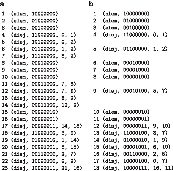
We implemented several algorithms in Java: (1) the algorithms of Arslan, (2) the algorithm of Chung et al., (3) our algorithm based on Four Russians based SLPs, and (4) our algorithm based on Steiner trees. The programs can be activated through a web interface and are also available for download via our web page http://www.cs.bgu.ac.il/∼http://negevcb/RL-CSA/index.php. We added to the preprocessing stage of the Four Russians based SLPs a trimming step, in which unused lines are removed from the SLP. Trimming an SLP can be done by locating all lines that take part in the construction of one of the required vectors in S (described in Subsection 2.1) and removing the rest (Fig. 6a,b).

Figure 6a,b shows an example of Four Russians based SLP construction and trimming. This example has Boolean vectors of length 8. The untrimmed SLP (Fig. 6a) has 23 lines, where the first 17 lines are block vector lines. The blocks are of length 3, so lines 1–7 enumerate all possible values in bits 0–2 (displayed left to right), lines 8–14 enumerate all possible values in bits 3–5, and lines 15–17 enumerate all possible values in the remaining bits 6–7. During the trimming step, five unused block vector lines are removed, yielding the trimmed SLP (Fig. 6b). For example, line 5 is not used in any disjunction operation nor is it one of the output vectors.

We compared the relative efficiency, as explained below, of heuristic Steiner minimal directed trees and Four Russians based SLPs as a function of NFA density (Fig. 7). To measure this, we randomly generated NFAs, constructed their corresponding data structures (Steiner minimal trees and SLPs) and measured their sizes. This simulation was repeated 100 times for each NFA size t, for different automata sizes t = 20, 40, 100, 160. We measured the relative efficiency of a data structure as 1 − N/|δ|, where N is its size (i.e., the size of the constructed Steiner directed tree, the length of the constructed Four-Russians SLP). The relative efficiencies of the different data structures were compared as a function of the density of the NFA. The density of the NFA equals |δ|/t². The random NFAs were constructed as follows. We created automata without transition labels, since they are irrelevant, and constructed only their graph structure. This is due to the fact that, at each step of the algorithm, transitions labeled by a single specific letter are used (see Eq. 3 and Eq. 4). We created an NFA transition table, where each transition exists with a probability of a randomly chosen density. Only NFAs with t reachable states were considered.

FIG. 7.

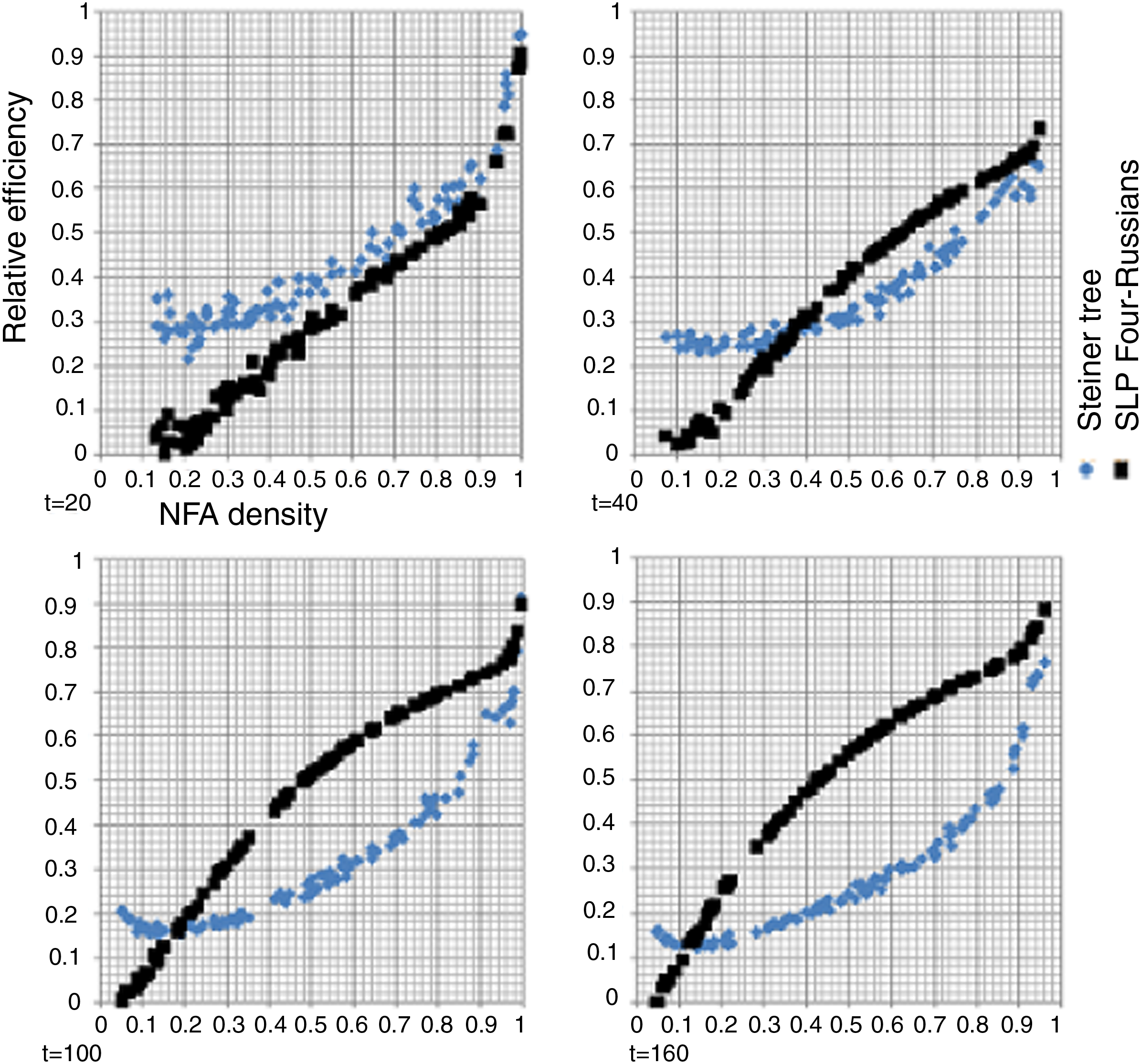
Efficiency comparison of different data structures as a function of NFA density. The simulation was repeated for number of states, t = 20, 40, 100, 160, each containing 100 randomly generated NFAs with t states and their corresponding data structures. Blue diamond, heuristic Steiner minimal directed tree; black square, SLP Four-Russians construction.

For each NFA, a Steiner directed tree was constructed, using the heuristic algorithms of Lin and Ni (1993) and Sheu and Yang (2001), with a minor modification that forces the constructed tree to be directed. Also, for each NFA, a corresponding Four-Russians based SLP was constructed, as described in Theorem 3, and then unused vectors were trimmed from it. Since the size of the trimmed Four-Russians based SLP is better than min \documentclass{aastex}\usepackage{amsbsy}\usepackage{amsfonts}\usepackage{amssymb}\usepackage{bm}\usepackage{mathrsfs}\usepackage{pifont}\usepackage{stmaryrd}\usepackage{textcomp}\usepackage{portland,xspace}\usepackage{amsmath,amsxtra}\pagestyle{empty}\DeclareMathSizes{10}{9}{7}{6} \begin{document} $$\min \ { { 2t^2 } / { \log t }, \mid \delta \mid \ } $$ \end{document} and the size of the Steiner tree is at most \documentclass{aastex}\usepackage{amsbsy}\usepackage{amsfonts}\usepackage{amssymb}\usepackage{bm}\usepackage{mathrsfs}\usepackage{pifont}\usepackage{stmaryrd}\usepackage{textcomp}\usepackage{portland,xspace}\usepackage{amsmath,amsxtra}\pagestyle{empty}\DeclareMathSizes{10}{9}{7}{6} \begin{document} $$ { t^2 } / { 4 } $$ \end{document} , it follows that, for large values of t, the SLP construction is better than the Steiner trees.

Our simulations show that both proposed data structures are smaller than the size of the transition table, which is a factor in the time complexity of the algorithm of Chung et al. Both have an increased efficiency as NFA density increases (Fig. 7). The heuristic Steiner minimal directed tree dominates for small values of t and low NFA density while the Four Russians SLP construction, described in Theorem 3, dominates for large values of t and high NFA density.

We conclude this section by demonstrating the performance of the three algorithmic approaches using part an example given in Chung et al. (2007a). The calculation of constrained sequence alignment on the AtGST and SsGST glutathione S-transferase (GST) sequences that appear in the example of Chung et al. (2007a), with regular expression constraint (S | T).2(D | E), yields 225370 max operations using our implementation of the algorithm of Chung et al., 211370 max operations using our Steiner tree based algorithm and 187606 max operations using our Four-Russians SLP based algorithm. The PAM250 scoring matrix, used in this example, gives a score of − 22. The alignment is given here:

AtGST:	-A-GIKVFGHPASIATRRVLIALHEKNLDFELVHVELKDGEHKKEPFLSRNPFGQ
SsGST:	PPYTITYFPVRGRCEAMRMLLADQDQSWK-EEV-VTM—E-TWPPLKPSCLFRQ
AtGST:	VPAFEDGDLKLFESRAITQYIAHRYENQGTNLLQTDS-KNISQY-AIMAIGMQVE
SsGST:	LPKFQDGDLTLYQSNAILRHLGRSFGLYGKDQKKEAALVDMDDNDGVEDLRCKYA
AtGST:	DHQFDP-VASKLAFEQIFKSIYGLTTDEAVVAEEEAKLAKVL–DV-Y-EARLKE
SsGST:	TLIYTNYEAGKEKYVKEL-PEH-LKPFETLLSQNQGGQAFVVGSQISFADYNLLD
AtGST:	-FKYLAGETF\|TLTD\|LHHIPAIQY
SsGST:	LLRIHQVLNP\|SCLD\|–AFP-L–

4. Conclusion

We have revisited the problem of Regular Language Constrained Sequence Alignment with focus on improving the dense NFA case. While Chung et al.'s algorithm yields O(n²|Q| · |δ|) = O(n²t³) time and O(n²t²) space, we achieved a bound of O(n²t³/logt) time and O(n²t²) space for the same problem. The above contribution is interesting when the input automaton is dense, i.e., when |δ| is asymptotically larger than \documentclass{aastex}\usepackage{amsbsy}\usepackage{amsfonts}\usepackage{amssymb}\usepackage{bm}\usepackage{mathrsfs}\usepackage{pifont}\usepackage{stmaryrd}\usepackage{textcomp}\usepackage{portland,xspace}\usepackage{amsmath,amsxtra}\pagestyle{empty}\DeclareMathSizes{10}{9}{7}{6} \begin{document} $$ { t^2 } / { \log t } $$ \end{document} .

We also implemented all four algorithms—Arslan (2007); Chung et al. (2007b), our SLP-based algorithm, and our Steiner-based algorithm—and made them available for public use on the Internet. Our experimental results, based on these implementations, indicate that the two approaches suggested in this article are also useful in practice.

We note that, in addition to the general result of Chung et al. mentioned above, they also gave an O(n²t² log t)-time algorithm for the special case where t = O(log n) and assuming a unit cost RAM model (Chung et al., 2007b). Our algorithm does not assume a unit cost RAM model nor any restriction on the ratio between the size of the automaton t and the length of the sequences n.

We further note that, in the case where the input is given in the form of a regular expression rather than an automaton, the complexity analysis of the algorithm can be expressed in terms of the length of the input regular expression. This is achieved based on recent algorithms which take as input a regular expression of length r and convert it into an ε-free NFA with O(r) states and O(r log ²r) transitions (Hromkoviěc et al., 2001; Schnitger, 2006; Geffert, 2003). This yields an O(n²r² log ²r) time and O(n²r²) space complexities for the algorithm of Chung et al. We note that this was not observed by Arslan and Egecioglu (2005) and Chung et al. (2007b).

Footnotes

Acknowledgments

We are grateful to Gregory Kabatiansky for his help on Theorem 2. The research of T.P. and M.Z.U. was partially supported by ISF (grant 478/10) and the Frankel Center for Computer Science at Ben Gurion University of the Negev.

Disclosure Statement

No competing financial interests exist.

References

Arslan

2007. Regular expression constrained sequence alignment. J. Discrete Algorithms, 5:647–661.

Arslan

, Egecioglu

2005. Algorithms for the constrained longest common subsequence problems. Int. J. Found. Comput. Sci., 16:1099–1110.

Bairoch

1993. The PROSITE dictionary of sites and patterns in proteins: its current status. Nucleic Acids Res., 21:3097.

Bern

, Plassmann

1989. The Steiner problem with edge lengths 1 and 2. Inform. Process. Lett., 32:171–176.

Chen

, Chao

2009. On the generalized constrained longest common subsequence problems. J. Combin. OptimOnline first10.1007/s10878-009-9262-5.

Chung

, Lee

, Tang

et al. 2007a. RE-MuSiC: a tool for multiple sequence alignment with regular expression constraints. Nucleic Acids Res., 35:W639.

Chung

, Lu

, Tang

2007b. Efficient algorithms for regular expression constrained sequence alignment. Inform. Process. Lett., 103:240–246.

Dinur

, Safra

2005. On the hardness of approximating minimum vertex cover. Ann. Math., 162:439–486.

Foulds

, Graham

1982. The Steiner problem in phylogeny is NP-complete. Adv. Appl. Math., 3:299.

10.

Geffert

2003. Translation of binary regular expressions into nondeterministic ɛ-free automata with O(n log n) transitions. J. Comput. Syst. Sci., 66:451–472.

11.

Gotthilf

, Hermelin

, Lewenstein

2008. Constrained lcs: Hardness and approximation. Lect. Notes Comput. Sci., 5029:255–262.

12.

Hromkoviěc

, Seibert

, Wilke

2001. Translating regular expressions into small ɛ-free nondeterministic finite automata. J. Comput. Syst. Sci., 62:565–588.

13.

Iliopoulos

, Rahman

2008. New efficient algorithms for the LCS and constrained LCS problems. Inform. Process. Lett., 106:13–18.

14.

Jia

, Han

, Au

et al. 2004. Optimal multicast tree routing for cluster computing in hypercube interconnection networks. IEICE Trans. Inform. Syst., E87-D:1625–1632.

15.

Lin

, Ni

1993. Multicast communication in multicomputer networks. IEEE Trans. Parallel Distributed Syst., 4:1105–1117.

16.

Peng

, Ting

2005. Time and space efficient algorithms for constrained sequence alignment. Lect. Notes Comput. Sci., 3317:237–246.

17.

Savage

1974. An algorithm for the computation of linear forms. SIAM J. Comput., 3:150–158.

18.

Schnitger

2006. Regular expressions and NFAs without ε-transitions. Lect. Notes Comput. Sci., 3884:432.

19.

Seberry

, Yamada

1992. Hadamard matrices, sequences, and block designs, 431–560. Dinitz

J.H.

, Stinson

D.R.

Contemporary Design Theory: A Collection of Surveys. Wiley–Interscience Series: New York.

20.

Sheu

, Yang

2001. Multicast algorithms for hypercube multiprocessors. J. Parallel Distributed Comput., 61:137–149.

21.

Shi

, Su

2006. The rectilinear Steiner arborescence problem is NP-complete. SIAM J. Comput., 35:729–740.

22.

Smith

, Waterman

1981. Identification of common molecular subsequences. J. Mol. Biol., 147:195–197.

23.

Sunyaev

, Bogopolsky

, Oleynikova

et al. 2004. From analysis of protein structural alignments toward a novel approach to align protein sequences. Proteins, 54:569–582.

24.

Sylvester

J.J.

1867. Thoughts on inverse orthogonal matrices, simultaneous sign successions, and tessellated pavements in two or more colours, with applications to Newton's rule, ornamental tile-work and the theory of numbers. Philosophical Magazine and Journal of Science, 34:461–475.

25.

Tang

, Lu

, Chang

et al. 2003. Constrained multiple sequence alignment tool development and its application to RNase family alignment. J. Bioinform. Comput. Biol., 1:267–287.

26.

Tsai

2003. The constrained longest common subsequence problem. Inform. Process. Lett., 88:173–176.