Discovery of Protein Complexes with Core-Attachment Structures from Tandem Affinity Purification (TAP) Data

Abstract

Many cellular functions involve protein complexes that are formed by multiple interacting proteins. Tandem Affinity Purification (TAP) is a popular experimental method for detecting such multi-protein interactions. However, current computational methods that predict protein complexes from TAP data require converting the co-complex relationships in TAP data into binary interactions. The resulting pairwise protein-protein interaction (PPI) network is then mined for densely connected regions that are identified as putative protein complexes. Converting the TAP data into PPI data not only introduces errors but also loses useful information about the underlying multi-protein relationships that can be exploited to detect the internal organization (i.e., core-attachment structures) of protein complexes. In this article, we propose a method called CACHET that detects protein complexes with Core-AttaCHment structures directly from bipartitETAP data. CACHET models the TAP data as a bipartite graph in which the two vertex sets are the baits and the preys, respectively. The edges between the two vertex sets represent bait-prey relationships. CACHET first focuses on detecting high-quality protein-complex cores from the bipartite graph. To minimize the effects of false positive interactions, the bait-prey relationships are indexed with reliability scores. Only non-redundant, reliable bicliques computed from the TAP bipartite graph are regarded as protein-complex cores. CACHET constructs protein complexes by including attachment proteins into the cores. We applied CACHET on large-scale TAP datasets and found that CACHET outperformed existing methods in terms of prediction accuracy (i.e., F-measure and functional homogeneity of predicted complexes). In addition, the protein complexes predicted by CACHET are equipped with core-attachment structures that provide useful biological insights into the inherent functional organization of protein complexes. Our supplementary material can be found at http://www1.i2r.a-star.edu.sg/∼xlli/CACHET/CACHET.htm ; binary executables can also be found there. Supplementary Material is also available at www.liebertonline.com/cmb .

1. Introduction

Protein complexes are molecular aggregations formed by simultaneous interactions among multiple proteins. Many important biological functions—such as DNA transcription, mRNA translation, signal transduction, and cell cycle—involve the formation of protein complexes. The RNA polymerase II complex and the nuclear pore complex are two such examples: the RNA polymerase II complex is needed for transcribing genetic information into messages for ribosomes to produce proteins (Cramer et al., 2000), while the nuclear pore complex is responsible for the protected exchange of components between the nucleus and cytoplasm, and for preventing the transport of material not destined to cross the nuclear membrane (Fahrenkrog and Aebi, 2003).

However, experimentally determined protein complex data are still largely obtained through small-scale experimental techniques, which are time-consuming and tedious. On the other hand, numerous high-throughput methods (e.g., yeast-two-hybrid and protein chips) for detecting binary protein-protein interactions (PPI) en masse have recently become available. By making use of the high-throughput PPI detection methods, a graphical map of an entire organism's interactome can be constructed from the PPI data by considering the individual proteins as the nodes, and a physical interaction between a pair of proteins as a link between the two corresponding nodes. It has been observed that protein complexes generally correspond to dense subgraphs or cliques in the PPI networks (Spirin and Mirny, 2003; Tong et al., 2002), as proteins in the same complex tend to be highly interactive with one another. This has given rise to many computational methods to detect protein complexes from the pairwise PPI data—for example, MCODE (Bader and Hogue, 2003), MCL (Pereira-Leal et al., 2004), DPCLus (Altaf-Ul-Amin et al., 2006), DECAFF (Li et al., 2007b), COACH (Wu et al., 2009), and CMC (Liu et al., 2009), just to name a few. A comprehensive survey of such methods can be found in Li et al. (2010).

As mentioned, protein complexes are formed by simultaneous interactions between multiple proteins. The above methods are based on experimental data that describe pairwise interactions between two proteins. For detecting multi-protein interactions, an increasingly popular experimental method is Tandem Affinity Purification (TAP). TAP exploits immobilized “bait” protiens to capture “prey” proteins that that interact with them, with the preys themselves in turn serving as baits for other preys, thereby capturing multi-protein interactions. Recently, several computational methods have been developed to analyze TAP data for protien complexes. However, they typically convert the co-complex relationships in TAP data into binary interactions. The resulting pairwise PPI network is then mined for densely connected regions that are identified as putative protein complexes. In coverting the TAP data into PPI data, the bait-prey relationships and even the prey-prey relationships are regarded as candidate PPIs which can be scored by various reliability measurements (Collins et al., 2007; Gavin et al., 2006; Zhang et al., 2008). The candidate interactions with scores above a pre-determined threshold are the predicted as true PPIs.

Clearly, the value of this threshold directly impact the quality of the resulting PPI network. Most of the proposed methods determine this threshold based on reference protein-complex data. For example, in Zhang et al. (2008) and Pu et al. (2007), the reference protein-complex PPI map is constructed by treating the connections between all proteins within the same complexes as known positive interactions and the connections between proteins from different complexes as negative interactions.1 Obviously, it is not reasonable to assume that all protein pairs within a complex are positive interactions. In a recent study, Friedel et al. (2008) presented an unsupervised strategy for converting TAP data into PPI data. First, preliminary PPI networks are constructed by sampling the original TAP data. Preliminary complexes are then predicted from these preliminary networks using Markov clustering algorithm (Pereira-Leal et al., 2004). The final PPI network, called the bootstrap network in the paper, is then constructed linking two proteins to form a PPI if they occur together in at least one preliminary complex. Clearly, current methods for converting the multi-protein TAP data into binary PPI data for protein complex detection are fairly awkward. The additional step of converting the TAP data into PPI data not only introduces errors but also loses useful information about the underlying multi-protein co-complex relationships (Puig et al., 2001) that can be useful for protein complex identification (Geva and Sharan, 2011; Scholtens et al., 2005). Direct detection of protein complexes from the TAP data is therefore much desired.

Furthermore, protein complexes have been found to contain core-attachment structures in which the cores are the functional “hearts” of the protein complexes, and the attachment proteins assist the core proteins to perform subordinate functions (Dezso et al., 2003; Gavin et al., 2006). While there are also several recent studies detecting core-attachment structures from PPI networks (Leung et al., 2009; Srihari et al., 2010; Wu et al., 2009), we believe that the co-complex information in the TAP data could be exploited to better detect the core-attachment structures in the protein complexes.

In this article, we introduce a novel method called CACHET to detect protein complexes with Core-AttaCHment structures directly from bipartitE TAP data. Instead of transforming the TAP data into a pairwise PPI network, we model the TAP data as a bipartite graph. The two vertex sets of the bipartite graph consist of the bait and prey proteins respectively, and the edges represent the bait-prey interactions. To detect the core-attachment structures in the protein complexes, our proposed method will focus first on the detection of high quality protein complex cores and then predicting the protein complexes by assembling attachments into the complex cores. To ensure the quality of the protein complex cores extracted from the TAP data, we compute the complete set of maximal bicliques from the bipartite graph and then extract those non-redundant reliable bicliques.

We performed extensive evaluation experiments on large-scale TAP data (Gavin et al., 2006; Krogan et al., 2006) and found that CACHET outperformed current methods in detecting protein complexes from these TAP data. In addition, we also evaluated the identified protein complexes and protein-complex cores using Gene Ontology (GO) functional information. The higher functional similarity found in the predicted complex cores is indicative of the biological significance of the protein complexes' structures detected by CACHET.

A newly proposed method called CODEC (Geva and Sharan, 2011) also detects protein complexes directly from TAP data as bipartite graphs. Our CACHET method works differently from CODEC in the following aspects. Firstly, CODEC detects dense bipartite subgraphs as protein complexes by iteratively adding proteins into seed subgraphs. Our CACHET selects protein-complex cores from bicliques and then simultaneously assembles all the attachments into cores to form the complexes. If we regard our cores as seed graphs, our approach for adding proteins into seed graphs to form protein complex is much more efficient than CODEC in terms of computation. Secondly, CACHET and CODEC address the issue of false positives in TAP data differently. CODEC approximates the reliability of bait-prey links mainly by the degree of the vertices. In contrast, CACHET exploits three state-of-the-art reliability measurements, such as Socio-Affinity (SA) (Gavin et al., 2006), Purification Enrichment (PE) (Collins et al., 2007), and Dice Coefficient (DC) (Zhang et al., 2008), which are demonstrated to assess the reliability of bait-prey relationships more accurately. As a result, our CACHET can detect protein complexes more efficiently, as well as with more biological significance (i.e., higher accuracy and homogeneity), than CODEC.

2. Preliminaries

As mentioned earlier, we represent TAP data as a bipartite graph G = (U, V, E), where U is the set of vertices for the baits, V the set of vertices for the preys captured by the baits in U, and E the bait-prey relationships. In addition, every edge \documentclass{aastex}\usepackage{amsbsy}\usepackage{amsfonts}\usepackage{amssymb}\usepackage{bm}\usepackage{mathrsfs}\usepackage{pifont}\usepackage{stmaryrd}\usepackage{textcomp}\usepackage{portland,xspace}\usepackage{amsmath,amsxtra}\pagestyle{empty}\DeclareMathSizes{10}{9}{7}{6}\begin{document}$$( u, v ) \in E$$\end{document} is associated with a reliability score that estimates the likelihood of the bait \documentclass{aastex}\usepackage{amsbsy}\usepackage{amsfonts}\usepackage{amssymb}\usepackage{bm}\usepackage{mathrsfs}\usepackage{pifont}\usepackage{stmaryrd}\usepackage{textcomp}\usepackage{portland,xspace}\usepackage{amsmath,amsxtra}\pagestyle{empty}\DeclareMathSizes{10}{9}{7}{6}\begin{document}$$u \in U$$\end{document} interacting with the prey \documentclass{aastex}\usepackage{amsbsy}\usepackage{amsfonts}\usepackage{amssymb}\usepackage{bm}\usepackage{mathrsfs}\usepackage{pifont}\usepackage{stmaryrd}\usepackage{textcomp}\usepackage{portland,xspace}\usepackage{amsmath,amsxtra}\pagestyle{empty}\DeclareMathSizes{10}{9}{7}{6}\begin{document}$$v \in V$$\end{document} .

Next, let us introduce some relevant concepts for a bipartite graph G. From G = (U, V, E), a biclique G′ = (U′, V′, E′) is a bipartite graph such that for any two vertices \documentclass{aastex}\usepackage{amsbsy}\usepackage{amsfonts}\usepackage{amssymb}\usepackage{bm}\usepackage{mathrsfs}\usepackage{pifont}\usepackage{stmaryrd}\usepackage{textcomp}\usepackage{portland,xspace}\usepackage{amsmath,amsxtra}\pagestyle{empty}\DeclareMathSizes{10}{9}{7}{6}\begin{document}$$u \in U^{ \prime}$$\end{document} and \documentclass{aastex} \usepackage{amsbsy} \usepackage{amsfonts} \usepackage{amssymb} \usepackage{bm} \usepackage{mathrsfs} \usepackage{pifont} \usepackage{stmaryrd} \usepackage{textcomp} \usepackage{portland, xspace} \usepackage{amsmath, amsxtra} \pagestyle{empty} \DeclareMathSizes {10} {9} {7} {6} \begin{document} $$v \in V^{ \prime}$$\end{document} , there is an edge \documentclass{aastex} \usepackage{amsbsy} \usepackage{amsfonts} \usepackage{amssymb} \usepackage{bm} \usepackage{mathrsfs} \usepackage{pifont} \usepackage{stmaryrd} \usepackage{textcomp} \usepackage{portland, xspace} \usepackage{amsmath, amsxtra} \pagestyle{empty} \DeclareMathSizes {10} {9} {7} {6} \begin{document} $$( u, v ) \in E^{ \prime}$$\end{document} , where U′, V′, and E′ are subsets of U, V, and E respectively. A biclique G₁ = (U₁, V₁, E₁) is a maximal biclique if there is no other biclique G₂ = (U₂, V₂, E₂) such that U₁ ⊆ U₂, V ₁ ⊆ V₂ and E₁ ⊆ E₂.

We define the reliability of a bipartite graph G = (U, V, E), R(G), as the average reliability scores of all the edges in E, \documentclass{aastex} \usepackage{amsbsy} \usepackage{amsfonts} \usepackage{amssymb} \usepackage{bm} \usepackage{mathrsfs} \usepackage{pifont} \usepackage{upgreek} \usepackage{stmaryrd} \usepackage{textcomp} \usepackage{portland, xspace} \usepackage{amsmath, amsxtra} \pagestyle{empty} \DeclareMathSizes{10}{9}{7}{6} \begin{document} \begin{align*}R ( G ) = \frac { \sum_ { u \neq v, ( u, v ) \in E } w ( u, v ) } { \sum_ { ( u, v ) \in E } \delta ( u, v ) }, \tag {1} \end{align*}\end{document}

where w(u, v) is the edge weight (reliability score) of the edge (u, v), and δ(u, v) is 0 if the vertices u and v are identical and 1 otherwise. The latter is because a bait together with a specific antibody tends to tag the bait itself as a prey in pull-down experiments; we do not want to consider edges in the form of (v, v) for calculating the reliability score in Equation (1) (Geva and Sharan, 2011).

Similarly, we can also define a reliability score for each vertex l in G called ratio_G(l) as follows: \documentclass{aastex} \usepackage{amsbsy} \usepackage{amsfonts} \usepackage{amssymb} \usepackage{bm} \usepackage{mathrsfs} \usepackage{pifont} \usepackage{upgreek} \usepackage{stmaryrd} \usepackage{textcomp} \usepackage{portland, xspace} \usepackage{amsmath, amsxtra} \pagestyle{empty} \DeclareMathSizes{10}{9}{7}{6} \begin{document} \begin{align*}ratio_ { G } ( l ) = \frac { \sum_ { u \neq l, ( u, l ) \in E } w ( u, l ) } { \sum_ { ( u, l ) \in E } \delta ( u, l ) }. \tag {2} \end{align*}\end{document}

We only use l's direct neighbors to compute its ratio score in Equation (2).

The Neighborhood affinity score (Bader and Hogue, 2003) is adopted to measure the similarity between two vertex sets. Given two bipartite graphs—G₁ = (U₁, V₁, E₁) and G₂ = (U₂, V₂, E₂)—we define their neighborhood affinity score, NA(G₁, G₂) as follows: \documentclass{aastex} \usepackage{amsbsy} \usepackage{amsfonts} \usepackage{amssymb} \usepackage{bm} \usepackage{mathrsfs} \usepackage{pifont} \usepackage{upgreek} \usepackage{stmaryrd} \usepackage{textcomp} \usepackage{portland, xspace} \usepackage{amsmath, amsxtra} \pagestyle{empty} \DeclareMathSizes{10}{9}{7}{6} \begin{document} \begin{align*}NA ( G_ { 1 }, G_ { 2 } ) = \frac { \mid ( U_ { 1 } \cup V_ { 1 } ) \cap ( U_ { 2 } \cup V_ { 2 } ) \mid ^2 } { \mid U_ { 1 } \cup V_ { 1 } \mid \times \mid U_ { 2 } \cup V_ { 2 } \mid }. \tag {3} \end{align*}\end{document}

Figure 1 provides an example TAP bipartite graph. The baits v₁ and v₂ together with the preys v₁, v₄, and v₅ form a biclique G′, with the reliability score \documentclass{aastex} \usepackage{amsbsy} \usepackage{amsfonts} \usepackage{amssymb} \usepackage{bm} \usepackage{mathrsfs} \usepackage{pifont} \usepackage{stmaryrd} \usepackage{textcomp} \usepackage{portland, xspace} \usepackage{amsmath, amsxtra} \pagestyle{empty} \DeclareMathSizes {10} {9} {7} {6} \begin{document} $$R ( G^ { \prime } ) = \frac { 0.7 + 0.6 + 0.65 + 0.9 } { 4 } = 0.71$$\end{document} . The protein v₁ as a bait has a \documentclass{aastex} \usepackage{amsbsy} \usepackage{amsfonts} \usepackage{amssymb} \usepackage{bm} \usepackage{mathrsfs} \usepackage{pifont} \usepackage{stmaryrd} \usepackage{textcomp} \usepackage{portland, xspace} \usepackage{amsmath, amsxtra} \pagestyle{empty} \DeclareMathSizes {10} {9} {7} {6} \begin{document} $$ratio ( v_ { 1 } ) = \frac { 0.6 + 0.65 } { 2 } = 0.625$$\end{document} , while it as a prey has a reliability score of 0.7. The reliability of this sample bipartite graph is 0.6 according to the Equation (1).

FIG. 1.

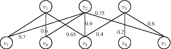
An example of a TAP bipartite graph.

3. Methods

Let us introduce our proposed algorithm CACHET to detect protein complexes and their core-attachment structures from TAP data. The key of our method is the detection of high-quality protein-complex cores. First, we compute the maximal bicliques in the TAP bipartite graph, since proteins within protein-complex cores are known to be highly interactive (Gavin et al., 2006). Next, we detect reliable protein-complex cores from the computed bicliques. Given the presence of false positive bait-prey interactions, we perform a filtering process to extract reliable bicliques (see Section 3.1). Since these reliable bicliques may have big overlaps with each other (i.e., they share many common proteins), we eliminate redundancy among these potential cores by computing a maximal independent set of them (see Section 3.2). The reliable and independent/non-redundant bicliques are predicted as the protein-complex cores. Finally, attachment proteins are included into the cores to form protein complexes with core-attachment substructures.

3.1. Mining reliable bicliques

We apply the FP-MBC algorithm (Li et al., 2007a) to compute the complete set of maximal bicliques from the bipartite TAP graph. We require that a detected maximal biclique should have at least Min_Bait baits and Min_Prey preys. In this study, both Min_Bait and Min_Prey are set as 2. We consider a biclique G′ to be reliable if its reliability score is greater than or equal to a threshold r, that is, R(G′) ≥ r. Reliable bicliques are likely to be protein-complex cores since most of their bait-prey interactions can be regarded to be true with respect to an appropriate threshold r.

Algorithm 1 shows the detailed steps for extracting reliable bicliques from the bipartite TAP graph G_TAP = (U_T, V_T, E_T). First, we compute the reliability scores for all the bait-prey edges in G_TAP. We exploit multiple state-of-the-art reliability measurements such as Socio-Affinity (SA) (Gavin et al., 2006), Purification Enrichment (PE) (Collins et al., 2007), and Dice Coefficient (DC)(Zhang et al., 2008) for accurate edge-weighting. We preserve a biclique if it is already reliable (Lines 3–4). If a biclique is of low reliability, we iteratively delete a vertex with the minimum ratio score (Lines 7–8) to increase its reliability and obtain a reliable bilcique if possible (Lines 10–11). The vertex removal process is guaranteed to increase or at least maintain the overall reliability of the biclique in each iteration (for a theoretical proof, see the appendix in our supplementary material at http://www1.i2r.a=star.edu.sg/∼xlli/CACHET/CACHET.htm; the binary executables can also be found there). Supplementary Material is also available at www.liebertonline.com/cmb. During this process, we also require that the vertices to be removed are selected from an available node set to guarantee that all the detected reliable bicliques satisfy the size constraint (i.e., they should have at least Min_Bait baits and Min_Prey preys). For example, if a biclique G′ = (U′, V′, E′) has a bait set with the minimum size (i.e., |U′| = Min_Bait) and the prey set is still large enough (i.e., |V′| > Min_Prey), we should select a vertex from the prey set and then remove it. The available node set in G′, denoted as A(G′), is defined in Equation (4): \documentclass{aastex} \usepackage{amsbsy} \usepackage{amsfonts} \usepackage{amssymb} \usepackage{bm} \usepackage{mathrsfs} \usepackage{pifont} \usepackage{upgreek} \usepackage{stmaryrd} \usepackage{textcomp} \usepackage{portland, xspace} \usepackage{amsmath, amsxtra} \pagestyle{empty} \DeclareMathSizes{10}{9}{7}{6} \begin{document} \begin{align*}A ( G^{ \prime} ) = \begin{cases}U^{ \prime} \cup V^{ \prime}, \quad { \rm if} \mid U^{ \prime} \mid > Min \_Bait, \mid V^{ \prime} \mid > Min \_Prey; \\ V^{ \prime}, \qquad \quad { \rm if} \mid U^{ \prime} \mid = Min \_Bait, \mid V^{ \prime} \mid > Min \_Prey; \\ U^{ \prime}, \qquad \quad { \rm if} \mid U^{ \prime} \mid > Min \_Bait, \mid V^{ \prime} \mid = Min \_Prey; \\ \phi, \qquad \quad \ { \rm Otherwise.}\end{cases} \tag{4}\end{align*}\end{document}

Note that our iterative removal process (Lines 6–9) will stop with the biclique in question being either preserved or discarded. If a biclique is reliable after the removal of some vertices, it will be preserved in Line 11 and the iteration stops. Otherwise, it will be discarded if it has reached the minimum size (i.e., A(G′) = ϕ), and yet it is still not reliable.

Algorithm 1

Mining reliable bicliques

Input: The set of bicliques from the FP-MBC algorithm,

r is the threshold for reliability score for reliable bicliques.

Output: The set of reliable bicliques, S.

1: Collect the reliability scores for all the bait-prey edges in G_TAP

2: for each biclique G′ = (U′, V′, E′) do

3: if R(G′) ≥ r

4: insert G′ into S

5: else

6: while R(G′) < r and A(G′) ≠ ϕ do

\documentclass{aastex} \usepackage{amsbsy} \usepackage{amsfonts} \usepackage{amssymb} \usepackage{bm} \usepackage{mathrsfs} \usepackage{pifont} \usepackage{stmaryrd} \usepackage{textcomp} \usepackage{portland, xspace} \usepackage{amsmath, amsxtra} \pagestyle{empty} \DeclareMathSizes {10} {9} {7} {6} \begin{document} $$v = \displaystyle \arg \min_{w \in A ( G^{ \prime} ) } ratio_{G^{\prime}} ( w )$$\end{document}

8: G′ = G′ − {v} //update G′ by deleting v and its corresponding edges

9: end while

10: if R(G′) ≥ r

11: insert G′ into S

12: end for

3.2. Mining maximal independent bicliques

The detected reliable bicliques may overlap with each other. As such, we need to select a maximal subset of independent/non-redundant bicliques as our protein-complex cores. To do so, we construct a redundancy graph, denoted as RG = (V_RG, E_RG, W), where the super vertex set \documentclass{aastex} \usepackage{amsbsy} \usepackage{amsfonts} \usepackage{amssymb} \usepackage{bm} \usepackage{mathrsfs} \usepackage{pifont} \usepackage{stmaryrd} \usepackage{textcomp} \usepackage{portland, xspace} \usepackage{amsmath, amsxtra} \pagestyle{empty} \DeclareMathSizes {10} {9} {7} {6} \begin{document} $$V_{RG} = \{ G_{i} \mid G_{i} \in S \} $$\end{document} consists of the reliable bicliques in S generated by Algorithm 1. While the bicliques are graphs themselves, we regard them as super vertices in our redundancy graph. The super edge set \documentclass{aastex} \usepackage{amsbsy} \usepackage{amsfonts} \usepackage{amssymb} \usepackage{bm} \usepackage{mathrsfs} \usepackage{pifont} \usepackage{stmaryrd} \usepackage{textcomp} \usepackage{portland, xspace} \usepackage{amsmath, amsxtra} \pagestyle{empty} \DeclareMathSizes {10} {9} {7} {6} \begin{document} $$E_{RG} = \{ ( G_{i}, G_{j} ) \| G_{i}, G_{j} \in V_{RG}, NA ( G_{i}, G_{j} ) \geq 0.2 \} $$\end{document} links two super vertices if these two reliable bicliques are deemed to be similar or redundant. In this work, two reliable bicliques are considered to be similar when their NA score (see Equation (3)) is at least 0.2, a value that was also used in many previous studies (Altaf-Ul-Amin et al., 2006; Bader and Hogue, 2003; Li et al., 2007b; Wu et al., 2009) to evaluate whether a predicted complex matches a benchmark complex.

The vertex weighting function W computes the significance of reliable bicliques as follows. First, we count the frequency of each vertex/protein in all the reliable bicliques to indicate their respective importance, given that proteins that appear in multiple modules are likely to be more biologically important (Navlakha and Kingsford, 2010) than those that do not. Equation (5) below computes w(u) as the importance score of the vertex/protein u, where the frequency of u, freq(u), is the number of reliable bicliques involving u: \documentclass{aastex} \usepackage{amsbsy} \usepackage{amsfonts} \usepackage{amssymb} \usepackage{bm} \usepackage{mathrsfs} \usepackage{pifont} \usepackage{upgreek} \usepackage{stmaryrd} \usepackage{textcomp} \usepackage{portland, xspace} \usepackage{amsmath, amsxtra} \pagestyle{empty} \DeclareMathSizes{10}{9}{7}{6} \begin{document} \begin{align*}w ( u ) = \frac { freq ( u ) } { \displaystyle \max_ { v } freq ( v ) } \tag { 5 } \end{align*}\end{document}

We refine the reliability score for bicliques in Equation (1) by considering the importance of vertices to evaluate the significance of reliable bicliques: \documentclass{aastex} \usepackage{amsbsy} \usepackage{amsfonts} \usepackage{amssymb} \usepackage{bm} \usepackage{mathrsfs} \usepackage{pifont} \usepackage{upgreek} \usepackage{stmaryrd} \usepackage{textcomp} \usepackage{portland, xspace} \usepackage{amsmath, amsxtra} \pagestyle{empty} \DeclareMathSizes{10}{9}{7}{6} \begin{document} \begin{align*}W ( G^ { \prime } ) = \frac { \sum_ { u \in U^ { \prime }, v \in V^ { \prime }, u \neq v } w ( u, v ) \times ( w ( u ) + w ( v ) ) } { 2 \times \sum_ { u \in U^ { \prime }, v \in V^ { \prime } } \delta ( u, v ) }, \tag { 6 } \end{align*}\end{document}

where G′ = (U′, V′, E′) is a reliable biclique, the edge weight w(u, v) is the edge reliability (Collins et al., 2007; Gavin et al., 2006; Zhang et al., 2008), and the vertex weight w(u) is the vertex u's importance as computed in Equation (5).

Given a redundancy graph RG = (V_RG, E_RG, W), our aim is to mine for an independent set (IS) in RG in which no two reliable bicliques are similar. This is a maximum independent set (MIS) problem. To conserve the more significant bicliques, we maximize the weight sum of the super vertices in the resulting independent set. Our MIS problem can thus be modeled as a maximum weighted independent set (MWIS) problem, as defined in Equation (7): \documentclass{aastex} \usepackage{amsbsy} \usepackage{amsfonts} \usepackage{amssymb} \usepackage{bm} \usepackage{mathrsfs} \usepackage{pifont} \usepackage{upgreek} \usepackage{stmaryrd} \usepackage{textcomp} \usepackage{portland, xspace} \usepackage{amsmath, amsxtra} \pagestyle{empty} \DeclareMathSizes{10}{9}{7}{6} \begin{document} \begin{align*}SC = \arg \max_{IS} \sum_{G_{i} \in IS}{W ( G_{i} ) }, \forall G_{j}, G_{k} \in IS, ( G_{j}, G_{k} ) \notin E_{RG}. \tag{7}\end{align*}\end{document}

Here, IS is an independent set of RG and the resulting set SC—the maximum weighted independent set—contains reliable and independent bicliques which form the set of our predicted protein-complex cores. Given a super vertex \documentclass{aastex} \usepackage{amsbsy} \usepackage{amsfonts} \usepackage{amssymb} \usepackage{bm} \usepackage{mathrsfs} \usepackage{pifont} \usepackage{stmaryrd} \usepackage{textcomp} \usepackage{portland, xspace} \usepackage{amsmath, amsxtra} \pagestyle{empty} \DeclareMathSizes {10} {9} {7} {6} \begin{document} $$v \in V_{RG}$$\end{document} , N_RG(v) is the set of v's neighbors in RG and its degree in RG, denoted as d_RG(v), is the cardinality of N_RG(v), i.e., |N_RG(v)|. The weighted degree of v is defined as \documentclass{aastex} \usepackage{amsbsy} \usepackage{amsfonts} \usepackage{amssymb} \usepackage{bm} \usepackage{mathrsfs} \usepackage{pifont} \usepackage{stmaryrd} \usepackage{textcomp} \usepackage{portland, xspace} \usepackage{amsmath, amsxtra} \pagestyle{empty} \DeclareMathSizes {10} {9} {7} {6} \begin{document} $$wd_{RG} ( v ) = \sum_{u \in N_{RG} ( v ) }W ( u )$$\end{document} . As we know, maximum independent set (MIS) and maximum weighted independent set (MWIS) are well-known NP-Complete problems (Garey and Johnson, 1979). Nonetheless, many approximation algorithms have been proposed for efficiently computing them. We introduce three heuristics in Algorithm 2 for mining the MWIS.

Algorithm 2

Maximum weighted independent set

Input: A weighted graph RG = (V_RG, E_RG, W).

Output: SC, a maximum weighted independent set in RG.

1: SC = ϕ, i = 0, T_i = RG

2: while V (T_i) ≠ ϕ do

3: select a vertex v_i based on one of the following criteria

\documentclass{aastex} \usepackage{amsbsy} \usepackage{amsfonts} \usepackage{amssymb} \usepackage{bm} \usepackage{mathrsfs} \usepackage{pifont} \usepackage{stmaryrd} \usepackage{textcomp} \usepackage{portland, xspace} \usepackage{amsmath, amsxtra} \pagestyle{empty} \DeclareMathSizes {10} {9} {7} {6} \begin{document} $$H_ { 1 } : \ v_ { i } = \arg \displaystyle \max_ { u \in V ( T_ {i} ) } \frac { W ( u ) } { d_ { T_ { i } } ( u ) + 1 } $$\end{document}

\documentclass{aastex} \usepackage{amsbsy} \usepackage{amsfonts} \usepackage{amssymb} \usepackage{bm} \usepackage{mathrsfs} \usepackage{pifont} \usepackage{stmaryrd} \usepackage{textcomp} \usepackage{portland, xspace} \usepackage{amsmath, amsxtra} \pagestyle{empty} \DeclareMathSizes {10} {9} {7} {6} \begin{document} $$H_ { 2 } : \ v_ { i } = \arg \displaystyle \max_ { u \in V ( T_ {i} ) } \frac { W ( u ) } { wd_ { T_ { i } } ( u ) } $$\end{document}

\documentclass{aastex} \usepackage{amsbsy} \usepackage{amsfonts} \usepackage{amssymb} \usepackage{bm} \usepackage{mathrsfs} \usepackage{pifont} \usepackage{stmaryrd} \usepackage{textcomp} \usepackage{portland, xspace} \usepackage{amsmath, amsxtra} \pagestyle{empty} \DeclareMathSizes {10} {9} {7} {6} \begin{document} $$H_{3} : \ v_{i} = \arg \displaystyle \max_{u \in V ( T_{i} ) } W ( u )$$\end{document}

\documentclass{aastex} \usepackage{amsbsy} \usepackage{amsfonts} \usepackage{amssymb} \usepackage{bm} \usepackage{mathrsfs} \usepackage{pifont} \usepackage{stmaryrd} \usepackage{textcomp} \usepackage{portland, xspace} \usepackage{amsmath, amsxtra} \pagestyle{empty} \DeclareMathSizes {10} {9} {7} {6} \begin{document} $$SC = SC \cup \{ v_{i} \}, T_{i + 1} = T_{i} - ( N_{T_{i}} ( v_{i} ) \cup \{ v_{i} \} ), i = i + 1$$\end{document}

//remove v_i, its neighbors and the corresponding edges from T_i.

8: end while

The first heuristic (H₁ in Line 4) (Sakai et al., 2003) greedily selects the super vertex with the maximum \documentclass{aastex} \usepackage{amsbsy} \usepackage{amsfonts} \usepackage{amssymb} \usepackage{bm} \usepackage{mathrsfs} \usepackage{pifont} \usepackage{stmaryrd} \usepackage{textcomp} \usepackage{portland, xspace} \usepackage{amsmath, amsxtra} \pagestyle{empty} \DeclareMathSizes {10} {9} {7} {6} \begin{document} $$ \frac { W ( u ) } { d_ { T_ { i } } ( u ) + 1 } $$\end{document} value in the evolving graph T_i. The selected vertex generally has a relatively large weight and a low degree. In other words, it keeps those significant and less-connected bicliques. The second heuristic (H₂ in Line 5) (Kako et al., 2005) does the same thing except that it uses the weighted degree in the denominator. The third heuristic (H₃ in Line 6) selects the super vertex with the maximum significance score. The performance (e.g., approximation ratio) of H₁ and H₂ have been well studied. For example, in a redundancy graph RG = (V_RG, E_RG, W), H₁ has been shown to output an independent set with weight sum of at least \documentclass{aastex} \usepackage{amsbsy} \usepackage{amsfonts} \usepackage{amssymb} \usepackage{bm} \usepackage{mathrsfs} \usepackage{pifont} \usepackage{stmaryrd} \usepackage{textcomp} \usepackage{portland, xspace} \usepackage{amsmath, amsxtra} \pagestyle{empty} \DeclareMathSizes {10} {9} {7} {6} \begin{document} $$\sum_{v \in V_{RG}} W ( v ) / ( d_{RG} ( v ) + 1 )$$\end{document} (Sakai et al., 2003). In terms of computation, H₃ is clearly the most efficient to compute since H₁ and H₂ need to update the degree and weighted degree for super vertices in each iteration, while there is no need for H₃ to do so.

3.3. Detecting protein-complex attachments

Given that we have detected independent reliable bicliques as protein-complex cores, let us now identify the attachment proteins. For a protein-complex core G_c = (U_c, V_c, E_c) detected from the bipartite TAP graph G_TAP = (U_T, V_T, E_T), we detect its bait-attachments and prey-attachments as follows. Given a prey protein \documentclass{aastex} \usepackage{amsbsy} \usepackage{amsfonts} \usepackage{amssymb} \usepackage{bm} \usepackage{mathrsfs} \usepackage{pifont} \usepackage{stmaryrd} \usepackage{textcomp} \usepackage{portland, xspace} \usepackage{amsmath, amsxtra} \pagestyle{empty} \DeclareMathSizes {10} {9} {7} {6} \begin{document} $$p \notin V_{c}$$\end{document} (the prey set), we construct a temporary graph TG = (U_c, {p}, E_tg), where \documentclass{aastex} \usepackage{amsbsy} \usepackage{amsfonts} \usepackage{amssymb} \usepackage{bm} \usepackage{mathrsfs} \usepackage{pifont} \usepackage{stmaryrd} \usepackage{textcomp} \usepackage{portland, xspace} \usepackage{amsmath, amsxtra} \pagestyle{empty} \DeclareMathSizes {10} {9} {7} {6} \begin{document} $$E_{tg} = \{ ( u, p ) \mid u \in U_{c}, ( u, p ) \in E_{T} \}$$\end{document} . The prey p is then a bait-attachment of G_c if it satisfies the following two constraints. First, it should interact with more than half of proteins in U_c (i.e., |E_tg| > 0.5 * | |U_c|). As we know, G_c is a biclique and every prey in V_c interacts with all the baits in U_c. We relax the connectivity constraint for selecting bait-attachments here because the attachments are generally less interactive than the proteins in the cores (Gavin et al., 2006). Second, the edges between p and p's neighbors in U_c should have an average reliability score larger than the threshold r (i.e., the reliability of TG, R(TG) ≥ r). The prey-attachments are detected in the same way.

The resulting protein complexes are then formed by combining the protein-complex cores and their bait-attachments and prey-attachments (Supplementary Material Figure 1 depicts how our CACHET works on an example TAP graph).

4. Experimental Results

Before we present our experimental results, let us introduce the evaluation metrics and the datasets used in our experiments.

4.1. Evaluation metrics and experimental data

Given a predicted complex p = (V_p, E_p) (V_p comprises the proteins in the core and attachments of p) and a real complex b = (V_b, E_b), we use their neighborhood affinity score, NA(p, b), to determine how well they match with each other. We consider them to be matching, if NA(p, b) ≥ ω. While ω has been typically set as 0.2 in numerous previous studies (Altaf-Ul-Amin et al., 2006; Bader and Hogue, 2003; Li et al., 2007b; Wu et al., 2009), some may feel that the value of 0.2 is too low and liberal. Therefore, we also tried different values of ω from 0.2 to 0.5 for a more comprehensive evaluation. Please note that 0.5 is quite a high and stringent value. For example, given two complexes both with six proteins, they are only considered to be matched with each other if they share at least five common proteins.

For overall comparison of the methods, we use Precision, Recall, and F-measure to evaluate the performance of various methods (Chua et al., 2008; Wu et al., 2009). Let P and B denote the sets of complexes predicted by a computational method and those in the benchmark complex set, respectively. Let N_cp be the number of predicted complexes in P that match at least one benchmark complex, and N_cb be the number of benchmark complexes in B that match at least one predicted complex. Equations (8) and (9) give the definitions of Precision, Recall, and F-measure: \documentclass{aastex} \usepackage{amsbsy} \usepackage{amsfonts} \usepackage{amssymb} \usepackage{bm} \usepackage{mathrsfs} \usepackage{pifont} \usepackage{upgreek} \usepackage{stmaryrd} \usepackage{textcomp} \usepackage{portland, xspace} \usepackage{amsmath, amsxtra} \pagestyle{empty} \DeclareMathSizes{10}{9}{7}{6} \begin{document} \begin{align*}Precision = \frac { N_ { cp } } { \mid P \mid } \quad { \rm and } \quad Recall = \frac { N_ { cb } } { \mid B \mid }, \tag {8} \end{align*}\end{document} \documentclass{aastex} \usepackage{amsbsy} \usepackage{amsfonts} \usepackage{amssymb} \usepackage{bm} \usepackage{mathrsfs} \usepackage{pifont} \usepackage{upgreek} \usepackage{stmaryrd} \usepackage{textcomp} \usepackage{portland, xspace} \usepackage{amsmath, amsxtra} \pagestyle{empty} \DeclareMathSizes{10}{9}{7}{6} \begin{document} \begin{align*}F - measure = \frac { 2 \times Precision \times Recall } { Precision + Recall }. \tag {9} \end{align*}\end{document}

Note that the matching pairs of complexes may have different NA scores that indicate different degrees of matching. This issue is not taken into consideration in the above definitions. As such, we have also conducted a protein-level evaluation (Liu et al., 2009) for the various methods (for details, see Table 3 in Supplementary Material).

We also use GO to evaluate the functional homogeneity of predicted protein complexes based on p-values (Li et al., 2010). The p-value of a predicted complex C with respect to a functional group F is defined in equation (10): \documentclass{aastex} \usepackage{amsbsy} \usepackage{amsfonts} \usepackage{amssymb} \usepackage{bm} \usepackage{mathrsfs} \usepackage{pifont} \usepackage{upgreek} \usepackage{stmaryrd} \usepackage{textcomp} \usepackage{portland, xspace} \usepackage{amsmath, amsxtra} \pagestyle{empty} \DeclareMathSizes{10}{9}{7}{6} \begin{document} \begin{align*}p - value = 1 - \sum_ {i = 0} ^ {k - 1} {\frac {\left(\begin {matrix} \mid F \mid \\ i \end {matrix} \right) \left(\begin {matrix} \mid V \mid - \mid F \mid \\ \mid C \mid - i\end {matrix} \right)} {\left( \begin {matrix} \mid V \mid \\ \mid C \mid \end {matrix} \right)}}, \tag {10}\end{align*}\end{document}

where C contains k proteins in F, and |V| is the total number of proteins in the TAP data. The p-value of a predicted complex is the smallest p-value over all the possible functional groups. As such, a predicted complex with a low p-value indicates that it is enriched by proteins from the same function group and it is thus likely to be a true protein complex. In our experiments, the p-values (with Bonferroni correction) of identified complexes are calculated using SGD's GO::TermFinder (Boyle et al., 2004).

We applied CACHET on two public large-scale TAP data, namely, the data of Gavin et al. (2006) and the data of Krogan et al. (2006). Let us denote Gavin et al.'s data and Krogan et al.'s data as G_gavin = (U_g, V_g, E_g) and G_krogan = (U_k, V_k, E_k), respectively. G_gavin contains 1993 baits, 2670 preys, and 19277 bait-prey links, whereas G_krogan contains 1999 baits, 5202 preys, and 47204 bait-prey links. We also generated a dataset by combining Gavin et al.'s data with Krogan et al.'s data, denoted as G_combined = (U_c, V_c, E_c), where U_c = U_g ∪ U_k, V_c = V_g ∪ V_k and E_c = E_g ∪ E_k. The combined dataset contains 2850 baits, 5337 preys, and 63631 bait-prey links. Table 1 shows the relevant statistics about these three datasets. The benchmark protein complexes were downloaded from Wodaklab (Pu et al., 2009). The catalogue is called CYC2008, and it contains 408 manually curated protein complexes. (GO was downloaded from http://geneontology.org.)

Table 1.

Details of TAP Datasets

Details	Gavin et al.'s data	Krogan et al.'s data	Combined data
No. of baits	1993	1999	2850
No. of preys	2670	5202	5337
No. of links	19277	47204	63631

4.2. Evaluation of predicted protein complexes

We focus on presenting our results on Gavin et al.'s data in this subsection. Similar results were obtained on Krogan et al.'s data, and they can be found in Section 3 in Supplementary Material. We will show the results of CACHET on the combined data in Section 4.6.

First, we computed the results using the three different MWIS heuristics with the parameter r set as 0.7 (see Algorithm 1 for r; we have also performed the sensitivity study of r in Section 4.4). The second column of Table 2 shows the number of protein complexes predicted by different MWIS heuristics. H₁ and H₂ predicted nearly the same number of protein complexes and achieved similar Precision. Compared with H₁ and H₂, H₃ obtained fewer protein complexes, but achieved a higher Precision with similar Recall and higher F-measure. Given that time complexity is a practical constraint that we have considered, we only report the results using H₃ in our CACHET hereafter, as CACHET with H₃ detects protein complexes most efficiently.

Table 2.

Performance for Various MWIS Heuristics Using SA Scores on Gavin et al.'s Data (ω = 0.2)

Methods	No. of complexes	Precision	Recall	F-measure
H ₁	437	0.643	0.439	0.521
H ₂	438	0.651	0.446	0.529
H ₃	369	0.678	0.441	0.534

We compared our CACHET with the existing state-of-the-art methods, namely, MCODE (Bader and Hogue, 2003), MCL (Friedel et al., 2008; Krogan et al., 2006; Pereira-Leal et al., 2004), DC-CM (Zhang et al., 2008), COACH (Wu et al., 2009), and CODEC (Geva and Sharan, 2011) (CODEC has two different weighting schemes, denoted as CODECw₀ and CODECw₁. For details, in terms of F-measure and p-values, see Geva and Sharan (2011).

As we need to transform the TAP data to PPI networks to run the traditional algorithms (MCODE, MCL, and COACH) in these networks, the method that we have used to convert TAP data to PPI networks (Zhang et al., 2008) can be found in Section 2 of Supplementary Material. Note that applying different reliability schemes will result in different PPI networks during the conversion process. That is, these three methods (MCODE, MCL, and COACH) may obtain different results using different reliability schemes (see Table 2 in Supplementary Material, which shows the PPI networks converted from TAP data and indicates that applying different reliability schemes on the same data will result in different PPI networks).

Figure 2 shows the F-measure of various methods using three different reliability schemes on the data of Gavin et al. Our CACHET with SA scores achieved the highest overall F-measure. CACHET also achieved the highest F-measure when using SA and DC scores when compared to the other methods using the same scoring schemes. When using PE scores, CACHET did not perform as well as MCL, which has a F-measure of 48.6% and is the best performer of existing methods over all scoring schemes. Our CACHET with SA scores is still 4.8% higher than MCL with PE scores.

FIG. 2.

Comparison among various methods employed on Gavin et al.'s data using different reliability schemes.

As SA scores are most widely used, Table 3 shows the details of the comparison among various methods using SA scores (some methods are independent of reliability measurements, such as DC-CM, CODEC, and the original results “Gavin” and “Gavin-Core” from Gavin et al. [2006]). The F-measure of our CACHET is 53.4%, which is 7.9%, 8.3%, and 11.4% higher than that of MCL, COACH, and CODEC w₁, respectively, the top three performers of the existing methods. Furthermore, CACHET is shown to perform better than CODEC in terms of all three measures, although CODEC also models TAP data as a bipartite graph as we do. In addition, we also show the running time of our CACHET on Gavin et al.'s data in Section 6 of Supplementary Material, which indicates that CACHET is computationally more efficient than CODEC.

Table 3.

Performance for Various Methods on Gavin et al.'s Data (ω = 0.2)

Methods	No. of complexes	Precision	Recall	F-measure
MCODE	136	0.632	0.257	0.366
MCL	302	0.483	0.429	0.455
DC-CM	851	0.249	0.424	0.314
CODEC w₀	1082	0.276	0.343	0.306
CODEC w₁	1005	0.417	0.424	0.420
COACH	346	0.540	0.387	0.451
Gavin	491	0.267	0.309	0.287
Gavin-Core	478	0.329	0.414	0.367
CACHET	369	0.678	0.441	0.534

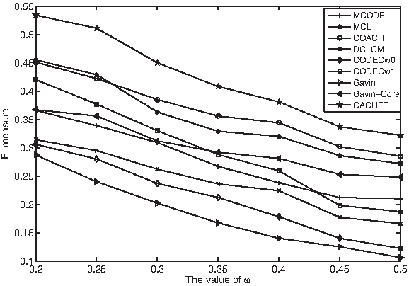
Finally, Figure 3 shows the F-measures of various methods when ω is varied from 0.2 to 0.5. CACHET consistently outperformed existing methods. This implies that the superiority of our CACHET is independent of the values of ω.

FIG. 3.

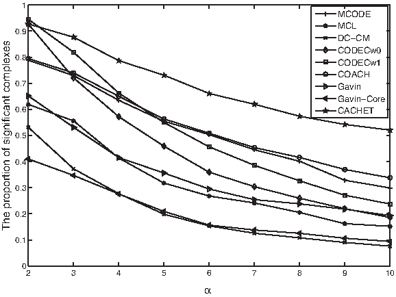
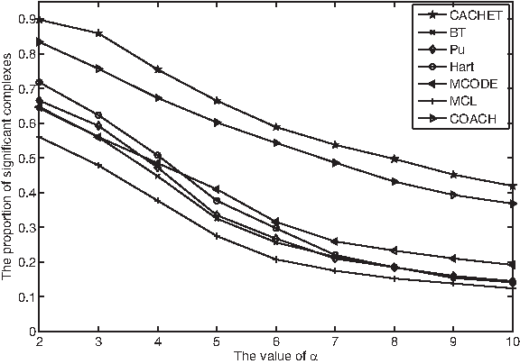
The proportion of significant complexes predicted by various methods.

We also investigate the proportion of protein complexes detected by the various methods that have statistically significant functional homogeneity. A protein complex has statistically significant functional homogeneity if its p-value is less than 10^−α the larger the α, the more likely that the complexes are genuine. Figure 4 shows the proportion of significant complexes under different values of α; In this figure,2 CACHET and CODEC (with both weighting schemes) are shown to achieve the highest proportion of significant complexes when α = 2. As the value of α increases, the superiority of our CACHET becomes obvious. For example, CACHET has 77.0% significant complexes, 10.7% higher than the second best (i.e., CODECw₁ with 66.3%) when α was set as 4. Furthermore, CACHET has 46.8% significant complexes, 13.0% higher than the second best (i.e., COACH with 33.8%) when α was set as 10. This shows that complexes predicted by CACHET are enriched by proteins with the same functions and are thus more likely to be true complexes.

FIG. 4.

F-measure of various methods when ω is varied from 0.2 to 0.5.

4.3. Evaluation of predicted protein-complex cores

Proteins within the complex cores have been found to have higher functional similarities and are more co-localized than the attachment proteins (Dezso et al., 2003; Gavin et al., 2006). For evaluation, we can calculate a functional similarity score for a core (or a protein complex) by averaging the semantic similarities among all bait-prey pairs (Wang et al., 2007). Table 4 shows the average functional similarity for all cores and protein complexes.

Table 4.

Average Functional Similarity Within Protein-Complex Cores and Protein Complexes

	Biological process (BP)		Cellular component (CC)
	in cores	In complexes	In cores	In complexes
H ₁	0.656 ± 0.008	0.601 ± 0.018	0.779 ± 0.006	0.762 ± 0.012
H ₂	0.675 ± 0.005	0.639 ± 0.016	0.796 ± 0.006	0.772 ± 0.008
H ₃	0.645 ± 0.010	0.582 ± 0.016	0.756 ± 0.007	0.724 ± 0.008

The functional similarities in Table 4 were calculated using two subontologies of GO (biological process and cellular component). The protein-complex cores generated by all three MWIS heuristics were found to have higher average functional similarities than the corresponding protein complexes. This demonstrates that our detected cores are more functionally consistent and likely to be more biologically significant. Figure 5 shows two examples to illustrate the organization of our predicted complexes. In Figure 5A, our identified core was reported in Gavin et al. (2006), and the predicted complex also matched well with the histone deacetylase complex (all eight proteins in our identified complexes are involved in the benchmark histone deacetylase complex). The protein YPL139C was identified as both bait-attachment and prey-attachment, and it is required to bind the protein YNL330C in the core for its activity. The protein YNL097C, which is predicted as another bait-attachment, has also been shown to be a possible component of the histone deacetylase complex (Gavin et al., 2006, 2002). In Figure 5B, the identified complex contained 14 proteins, which covered 10 of the 12 proteins in the benchmark DNA-directed RNA polymerase II complex (Cramer et al., 2000). The other four proteins in gray (YDL115C, YGR005C, YGR186C, and YML010W) are novel to our benchmark complex. However, YDL115C has already been demonstrated to belong to the DNA-directed RNA polymerase II complex (Krogan et al., 2006). The other three proteins identified as attachments were all annotated with the term GO:0006366 (transcription from RNA polymerase II promoter), which is also closely related to the function of this complex. This example indicates that our CACHET may be used to detect the potential knowledge absent in current reference data. Our identified core with the seven proteins was also validated in Gavin et al. (2006).

Fig. 5.

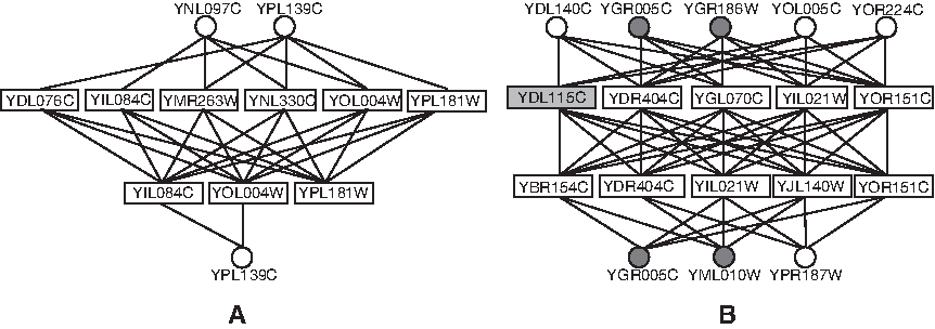
The organization of our identified protein complexes. The predicted complexes are histone deacetylase complex in (A) and DNA-directed RNA polymerase II complex in (B).

4.4. Effect of the parameter r

The reliability parameter r in Algorithm 1 determines the number and quality of the protein-complex cores detected by our CACHET. We investigate how the variation of r affects the performance of our CACHET. Figure 6 shows the Precision, Recall, and F-measure of CACHET on Gavin et al.'s data under different values of r.

FIG. 6.

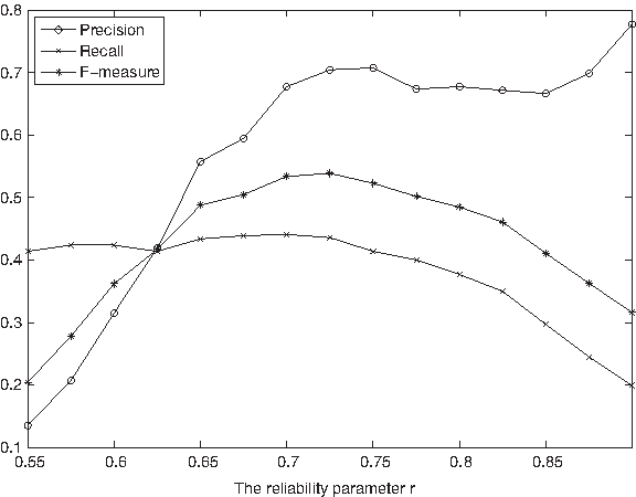
Performance of our CACHET method used on Gavin et al.'s data under different values of r.

Fewer false positive bait-prey links are involved in our identified complexes as we increase the reliability value of r, as expected. The predicted complexes are thus more likely to be true complexes, as reflected by the ascending trend of the precision of CACHET when r becomes larger, as shown in Figure 6. On the other hand, when r becomes too large, CACHET may filter away some true positive bait-prey interactions. As such, it will predict a small number of complexes with a low recall but achieving a very high precision. Overall, the resulting curve for the F-measure in Figure 6 has three distinct ranges. It increases significantly in the first range ( \documentclass{aastex} \usepackage{amsbsy} \usepackage{amsfonts} \usepackage{amssymb} \usepackage{bm} \usepackage{mathrsfs} \usepackage{pifont} \usepackage{stmaryrd} \usepackage{textcomp} \usepackage{portland, xspace} \usepackage{amsmath, amsxtra} \pagestyle{empty} \DeclareMathSizes {10} {9} {7} {6} \begin{document} $$r \in [ 0.55, 0.65 ]$$\end{document} ), remains stable in the second range ( \documentclass{aastex} \usepackage{amsbsy} \usepackage{amsfonts} \usepackage{amssymb} \usepackage{bm} \usepackage{mathrsfs} \usepackage{pifont} \usepackage{stmaryrd} \usepackage{textcomp} \usepackage{portland, xspace} \usepackage{amsmath, amsxtra} \pagestyle{empty} \DeclareMathSizes {10} {9} {7} {6} \begin{document} $$r \in [ 0.65, 0.8 ]$$\end{document} ), and decreases drastically in the last range. As such, in our experiments, we set r = 0.7 on Gavin et al.'s data to filter false positive interactions effectively while retaining most of true bait-prey relationships. For the other datasets and reliability measurements and to see how we select the value of r, see Section 5 in Supplementary Material.

4.5. Impact of reliability indexing and redundancy filtering

Recall that indexing the reliability of bait-prey links to identify reliable bicliques (denoted as Step I; see Section 3.1) and filtering redundancy amongst the detected reliable bicliques (denoted as Step II; see Section 3.2) are two key steps in CACHET. To see the impact of reliability indexing and redundancy filtering, we performed experiments to run CACHET without each step, respectively. In Table 5, CACHETwoI and CACHETwoII denote CACHET without Step I and Step II, respectively. CACHETwoI was observed to achieve a much lower precision than CACHET and CACHETwoII, indicating that detecting reliable bicliques does filter false positives effectively and increase the reliability of resulting protein complexes. Although CACHETwoII has the highest recall, it predicts protein complexes with huge redundancy (e.g., 4576/188 = 24.3 predicted complexes match a real one on average). The results showed that these two steps in CACHET are indeed essential to filter potential false positive interactions and reduce redundancy among protein-complexes.

Table 5.

Performance for CACHET on Gavin et al.'s Data (ω = 0.2)

Methods	No. of complexes	N_cp	N_cb	Precision	Recall	F-measure
CACHETwoI	3126	163	174	0.052	0.427	0.093
CACHETwoII	9862	4576	188	0.464	0.461	0.462
CACHET	369	250	180	0.678	0.441	0.534

4.6. Running CACHET on the combined data

Currently, Gavin et al. (2006) and Krogan et al. (2006) have already provided comprehensive TAP data. However, they just produced quite different descriptions of the yeast interactome due to the fact that they exploited different purification techniques and utilized a different number of baits in their purifications. Therefore, combining these two data sources will definitely improve the coverage of the data for better identifying protein complexes (Friedel et al., 2008; Hart et al., 2007; Pu et al., 2007).

Assuming that G_gavin = (U_g, V_g, E_g) and G_krogan = (U_k, V_k, E_k) denote Gavin et al.'s and Krogan et al.'s data, respectively, G_combined = (U_c, V_c, E_c) is the resulting combined data, where U_c = U_g ∪ U_k, V_c = V_g ∪ V_k, and E_c = E_g ∪ E_k. To index the reliability scores of edges in E_c, it is a possible solution to re-compute these scores based on the purification records in the combined data. Here, we adopt the strategy used in Collins et al. (2007) to assign reliability scores for bait-prey links in the combined data based on their original scores in individual datasets. For an edge \documentclass{aastex} \usepackage{amsbsy} \usepackage{amsfonts} \usepackage{amssymb} \usepackage{bm} \usepackage{mathrsfs} \usepackage{pifont} \usepackage{stmaryrd} \usepackage{textcomp} \usepackage{portland, xspace} \usepackage{amsmath, amsxtra} \pagestyle{empty} \DeclareMathSizes {10} {9} {7} {6} \begin{document} $$e \in E_c$$\end{document} , w_k(e) and w_g(e) are its scores in Krogan et al.'s data, and Gavin et al.'s data respectively. w_c(e), its score in the combined data, is calculated the same as PE scores by a weighted sum of w_k(e) and w_g(e) in Equation (11) instead of a straight sum, as suggested by Collins et al. (2007): \documentclass{aastex} \usepackage{amsbsy} \usepackage{amsfonts} \usepackage{amssymb} \usepackage{bm} \usepackage{mathrsfs} \usepackage{pifont} \usepackage{upgreek} \usepackage{stmaryrd} \usepackage{textcomp} \usepackage{portland, xspace} \usepackage{amsmath, amsxtra} \pagestyle{empty} \DeclareMathSizes{10}{9}{7}{6} \begin{document} \begin{align*}w_{c} ( e ) = 0.5 \times w_{k} ( e ) + w_{g} ( e ). \tag{11}\end{align*}\end{document}

We compared our CACHET with existing methods: MCODE, MCL, COACH, the bootstrapping method (BT) (Friedel et al., 2008), Pu et al.'s method (Pu et al., 2007), and Hart et al.'s method (Hart et al., 2007). Since the last three methods are independent of scoring schemes, we first show the F-measure of CACHET, MCODE, MCL, and COACH using various scoring schemes in Figure 7. The result is very similar to that of Gavin et al.'s data (Fig. 2). In terms of using individual scoring schemes, CACHET achieved the highest F-measure when using SA and DC scores, and performed equally well as MCL when using PE scores. In particular, CACHET with SA scores achieved the highest F-measure as compared to other methods with any scoring schemes. For example, CACHET with SA scores has an F-measure of 61.5%, (5.5% higher than MCL with PE scores), which is the best performer by combining existing methods and scoring schemes.

FIG. 7.

Comparison among various methods employed on the combined data using different reliability schemes.

CACHET with SA scores predicted 449 protein complexes from the combined data (the reliability threshold is set as 0.7, which is the same as on the Gavin et al.'s data). Compared with the results from individual data, CACHET achieved higher Precision, Recall, and F-measure on the combined data as shown in Table 6, indicating that CACHET can effectively exploit the biological knowledge from multiple data. Table 7 shows the comparison details between our CACHET using SA scores and other methods on the combined data. While MCL, BT, Pu, and Hart were shown to obtain relatively high recall, our CACHET gained much higher Precision, and thus obtained the highest overall F-measure. Our higher Precision indicates that the complexes predicted by CACHET are more accurate, implying that our unmatched complexes are more likely to be novel true complexes. We also show the F-measure of the above methods with different values of ω in Figure 8 and observe that our CACHET consistently achieved the best overall performance even with more stringent matching criteria.

FIG. 8.

Performance of our CACHET method used on Gavin et al.'s data under different values of ω.

Table 6.

Performance of Various Methods Using SA Scores on Combined Data (ω = 0.2)

Data	No. of complexes	N_cp	N_cb	Precision	Recall	F-measure
Gavin	369	250	180	0.678	0.441	0.534
Krogan	404	254	172	0.629	0.422	0.506
Combined	449	343	210	0.764	0.515	0.615

Table 7.

CACHET on Combined Data Using SA Scores (ω = 0.2)

Method	No. of complexes	N_cp	N_cb	Precision	Recall	F-measure
CACHET	449	343	210	0.764	0.515	0.615
BT	409	204	244	0.499	0.598	0.544
Pu	400	201	241	0.503	0.591	0.543
Hart	390	203	242	0.521	0.593	0.554
MCODE	265	123	149	0.462	0.365	0.408
MCL	1076	236	270	0.219	0.662	0.329
COACH	439	221	174	0.502	0.426	0.462

Finally, for functional homogeneity, Figure 9 shows the proportion of statistically significant complexes from the combined data under different values of α. Our CACHET is again observed to consistently achieve the highest proportion of statistically significant complexes. For example, when α was set as 2, CACHET produced 89.8% significant complexes, which is 6.4%, 18%, and 23.3% higher than COACH, Hart, and Pu (the top three performers), respectively.

FIG. 9.

The proportion of significant complexes predicted by various methods from the combined data.

5. Conclusion

In this article, we have proposed a novel algorithm CACHET to detect protein complexes as well as their core-attachment structures from TAP data. CACHET first computes all the maximal bicliques from the TAP bipartite graph. It detects high-quality protein-complex cores from the computed maximal bicliques by extracting reliable bicliques and removing redundancy among them. Then, CACHET forms protein complexes by incorporating attachments into cores.

CACHET significantly outperformed existing methods in terms of the F-measure and functional homogeneity of predicted complexes. Experimental evaluation on our identified protein complexes and cores also demonstrated the following advantages of our CACHET. First, as CACHET detects protein complexes directly from TAP data, it is able to exploit the co-complex information in the TAP data and avoid the step of converting the TAP data into a binary PPI network. Second, the protein complexes predicted by CACHET are with core-attachment structures, which provide useful information for revealing the inherent organization of the detected protein complexes.

Footnotes

Acknowledgment

This article was supported by Singapore MOE AcRF grant no. MOE2008-T2-1-074.

Disclosure Statement

No competing financial interests exist.

1

An additional restriction—cellular localization—was used for defining negative interactions in Pu et al. ().

2

Please note that the singleton complexes (those with only one protein) are not considered for p-value calculation (Wu et al., ).

References

Altaf-Ul-Amin

, Shinbo

, Mihara

et al. 2006. Development and implementation of an algorithm for detection of protein complexes in large interaction networks. BMC Bioinform., 7:207.

Bader

, Hogue

2003. An automated method for finding molecular complexes in large protein interaction networks. BMC Bioinform., 4:2.

Boyle

E.I.

, Weng

, Gollub

et al. 2004. GO::TermFinder—open source software for accessing gene ontology information and finding significantly enriched gene ontology terms associated with a list of genes. Bioinformatics, 20:3710–3715.

Chua

H.N.

, Ning

, Sung

W.-K.

et al. 2008. Using indirect protein-protein interactions for protein complex prediction. J. Bioinform. Comput. Biol., 6:435–466.

Collins

S.R.

, Kemmeren

, Zhao

X.C.

et al. 2007. Toward a comprehensive atlas of the physical interactome of saccharomyces cerevisiae. Mol. Cell Proteomics, 6:439–450.

Cramer

, Bushnell

D.A.

, Fu

et al. 2000. Architecture of RNA polymerase ii and implications for the transcription mechanism. Science, 288:640–649.

Dezso

, Oltvai

Z.D.

, Barabasi

A.L.

2003. Bioinformatics analysis of experimentally determined protein complexes in the yeast Saccharomyces cerevisiae. Genome Res., 13:2450–2454.

Fahrenkrog

, Aebi

2003. The nuclear pore complex: nucleocytoplasmic transport and beyond. Nat. Rev. Mol. Cell Biol, 4,10:757–766.

Friedel

C.C.

, Krumsiek

, Zimmer

2008. Boostrapping the interactome: unsupervised identification of protein complexes in yeast. Lect. Notes Comput. Sci., 4955:3–16.

10.

Garey

M.R.

, Johnson

D.S.

1979. Computers and Intractability; A Guide to the Theory of NP-Completeness. W. H. Freeman & Co.: New York.

11.

Gavin

A.C.

, Bösche

, Krause

et al. 2002. Functional organization of the yeast proteome by systematic analysis of protein complexes. Nature, 415:141–147.

12.

Gavin

, Aloy

, Grandi

et al. 2006. Proteome survey reveals modularity of the yeast cell machinery. Nature, 440:631–636.

13.

Geva

, Sharan

2011. Identification of protein complexes from co-immunoprecipitation data. Bioinformatics, 27:111–117.

14.

Hart

G.T.

, Lee

, Marcotte

2007. A high-accuracy consensus map of yeast protein complexes reveals modular nature of gene essentiality. BMC Bioinform., 8:236.

15.

Kako

, Ono

, Hirata

et al. 2005. Approximation algorithms for the weighted independent set problem. Lect. Notes Comput. Sci., 3787:341–350.

16.

Krogan

, Cagney

, Yu

et al. 2006. Global landscape of protein complexes in the yeast Saccharomyces cerevisiae. Nature, 440:637–643.

17.

Leung

H.C.

, Yiu

S.M.

, Xiang

et al. 2009. Predicting protein complexes from PPI data: a core-attachment approach. J. Comput. Biol., 16:133–144.

18.

, Liu

, Li

et al. 2007a. Maximal biclique subgraphs and closed pattern pairs of the adjacency matrix: a one-to-one correspondence and mining algorithms. IEEE Trans. Knowl. Data Eng., 19:1625–1637.

19.

, Foo

, Ng

2007b. Discovering protein complexes in dense reliable neighborhoods of protein interaction networks. Proc. CSB, 157–168.

20.

X.L.

, Wu

, Kwoh

C.K.

et al. 2010. Computational approaches for detecting protein complexes from protein interaction networks: a survey. BMC Genomics, 11:S3.

21.

Liu

G.M.

, Chua

H.N.

, Wong

2009. Complex discovery from weighted PPI networks. Bioinformatics, 25:1891–1897.

22.

Navlakha

, Kingsford

2010. Exploring biological network dynamics with ensembles of graph partitions. Proc. PSB, 166–177.

23.

Pereira-Leal

J.B.

, Enright

A.J.

, Ouzounis

C.A.

2004. Detection of functional modules from protein interaction networks. Proteins, 54:49–57.

24.

, Vlasblom

, Emili

et al. 2007. Identifying functional modules in the physical interactome of Saccharomyces cerevisiae. Proteomics, 7:944–960.

25.

, Wong

, Turner

et al. 2009. Up-to-date catalogues of yeast protein complexes. Nucleic Acids Res., 37:825–831.

26.

Puig

, Caspary

, Rigaut

G.G.R.

et al.2001. The tandem affinity purification (TAP) method: a general procedure of protein complex purification. Methods, 24:218–229.

27.

Sakai

, Togasaki

, Yamazaki

2003. A note on greedy algorithms for the maximum weighted independent set problem. Discrete Appl. Math., 126:313–322.

28.

Scholtens

, Vidal

, Gentleman

2005. Local modeling of global interactome networks. Bioinformatics, 21:3548–3557.

29.

Spirin

, Mirny

2003. Protein complexes and functional modules in molecular networks. Proc. Natl. Acad. Sci. USA, 100:12123–12128.

30.

Srihari

, Ning

, Leong

H.W.

2010. MCL-CAW: a refinement of MCL for detecting yeast complexes from weighted PPI networks by incorporating core-attachment structure. BMC Bioinform., 11:504.

31.

Tong

, Drees

, Nardelli

et al. 2002. A combined experimental and computational strategy to define protein interaction networks for peptide recognition modules. Science, 295:321–324.

32.

Wang

, Du

, Payattakool

et al. 2007. A new method to measure the semantic similarity of go terms. Bioinformatics, 23:1274–1281.

33.

, Li

X.L.

, Kwoh

C.K.

et al. 2009. A core-attachment based method to detect protein complexes in ppi networks. BMC Bioinform., 10:169.

34.

Zhang

, Park

, Karpinets

T.V.

et al. 2008. From pull-down data to protein interaction networks and complexes with biological relevance. Bioinformatics, 24:979–986.

Supplementary Material

Please find the following supplemental material available below.

For Open Access articles published under a Creative Commons License, all supplemental material carries the same license as the article it is associated with.

For non-Open Access articles published, all supplemental material carries a non-exclusive license, and permission requests for re-use of supplemental material or any part of supplemental material shall be sent directly to the copyright owner as specified in the copyright notice associated with the article.

0.00 MB

0.10 MB