Adjustable Chain Trees for Proteins

Abstract

A chain tree is a data structure for changing protein conformations. It enables very fast detection of clashes and free energy potential calculations. A modified version of chain trees that adjust themselves to the changing conformations of folding proteins is introduced. This results in much tighter bounding volume hierarchies and therefore fewer intersection checks. Computational results indicate that the efficiency of the adjustable chain trees is significantly improved compared to the traditional chain trees.

1. Introduction

A chain tree is a data structure for fast clash detection and free energy maintenance of folding protein chains. Suppose that during the simulation of the folding process, an attempt to rotate a backbone or a side chain bond is made. Such a rotation should be undone if it results in a clash (either at some intermediate stage during the rotation or at the end of the rotation). Clashing rotations have to be identified and rejected as quickly as possible. If a rotation is not clashing, the free energy of the new conformation has to be estimated. This energy estimate is crucial for the decision if the rotation should be accepted or rejected (note that in many methods, the increase of the free energy is not always causing a rejection).

The chain tree is a binary tree where leaves are atom groups and each node is associated with a transform matrix and a bounding volume. To maintain the conformation of a protein chain during folding, a brute-force method can be employed. It requires Θ(n) update time for each conformational change and Θ(n²) time for each clash detection. Often, grid methods are used to reduce the clash detection time to Θ(n). Lotan et al. (2004) showed that, using chain trees, the update time can be reduced to \documentclass{aastex}\usepackage{amsbsy}\usepackage{amsfonts}\usepackage{amssymb}\usepackage{bm}\usepackage{mathrsfs}\usepackage{pifont}\usepackage{stmaryrd}\usepackage{textcomp}\usepackage{portland,xspace}\usepackage{amsmath,amsxtra}\pagestyle{empty}\DeclareMathSizes{10}{9}{7}{6} \begin{document} $${ \cal O} ( \log n )$$\end{document} with a Θ(n^4/3) clash-detection time. It was also demonstrated that the average CPU-time required to perform a step in a Monte-Carlo search was much lower when using a chain tree compared to using grids.

We suggest a modification of chain trees based on the assumption that portions of folding proteins (such as α-helices and β-strands) are formed relatively early in the folding process. They remain stable throughout many (if not all) iterations of the simulation. Bonds of such subchains can be locked, and the bounding volumes of these subchains will therefore remain unchanged. As a consequence, the chain tree can be rearranged (so that bounding volumes of locked subchains can be made tighter) and rebalanced (so that updates due to rotations of unlocked bonds can be carried out more efficiently). In addition, we exploit the property of peptide planes (backbone atoms between two consecutive C_α-atoms are always in the same plane) to obtain tight bounding volumes at the lower levels of chain trees. We provide computational results that clearly indicate increased efficiency of chain trees when rearrangements and rebalancing is applied. Relative improvements (cost speed-up over cost in regular chain trees) for tested protein chains on adjustable chain trees compared to regular chain trees were 16–63%. The average relative improvement was 36%. This substantial improvement was achieved without affecting the worst-case asymptotic time and space complexity. Since chain trees are already shown to be superior to grid methods, we do not compare adjustable chain trees to grid methods.

This article is organized as follows: A brief discussion of proteins with special emphasis on issues related to the chain trees is given in Section 2. Chain trees are described in Section 3. Sections 4–6 discuss how the structure of chain trees can be modified in order to exploit special properties of proteins. Bounding volumes used in the experiments are described in Section 7. Computational results are given in Section 8. Finally, concluding remarks and suggestions for further research are collected in Section 9.

2. Proteins

A protein is an organic compound made of n amino acids, \documentclass{aastex}\usepackage{amsbsy}\usepackage{amsfonts}\usepackage{amssymb}\usepackage{bm}\usepackage{mathrsfs}\usepackage{pifont}\usepackage{stmaryrd}\usepackage{textcomp}\usepackage{portland,xspace}\usepackage{amsmath,amsxtra}\pagestyle{empty}\DeclareMathSizes{10}{9}{7}{6} \begin{document} $$A_1 , A_2 , \ldots , A_n$$\end{document} , arranged in a linear chain. It folds into a three-dimensional (3D) structure referred to as the native conformation. Each amino acid is a molecule containing an amine group NH₂, a carboxylic acid group COOH, and a side chain R that varies for each of the 20 different amino acids. The amine group, the carboxyl group, the side chain, and the hydrogen atom are all covalently bonded to the carbon atom, denoted by C_α. The i-th amino acid A_i, 1 ≤ i < n, is joined with its successor A_i₊₁ by a peptide bond between the carboxyl group of A_i and the amine group of A_i₊₁ (Fig. 1). The carboxyl group is replaced by the C = O group, and the amine group is replaced by the NH group. Finally, a water molecule is formed during this polymerization of consecutive amino acids.

FIG. 1.

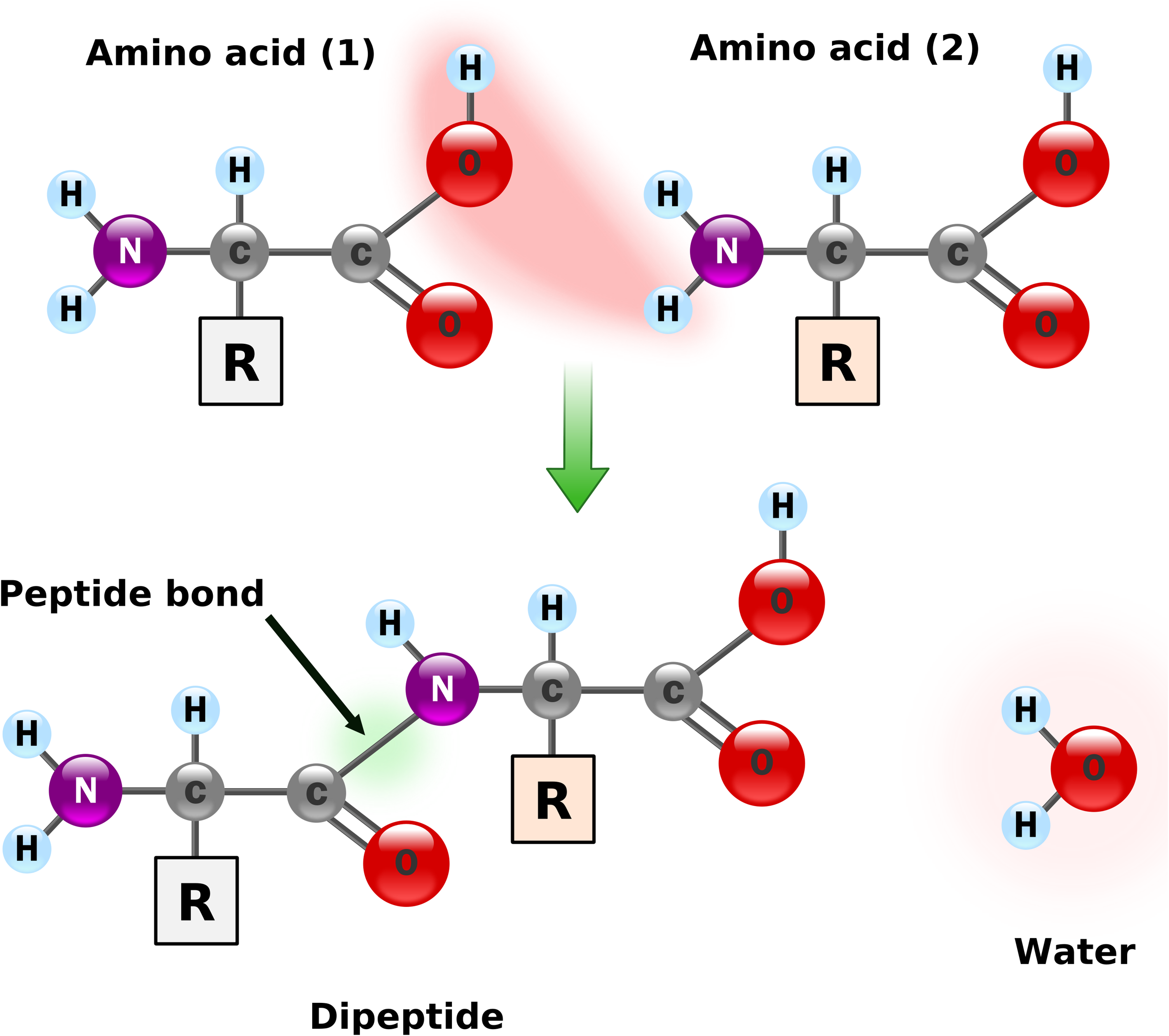
Peptide formation. Two amino acids form a peptide bond and a water molecule.

Once linked, individual amino acids are referred to as residues, and the chain of consecutive N-, C_α-, and C-atoms (sometimes together with the O-atom attached the C-atom and the H-atom attached to the N-atom) is the backbone of the protein.

Bond lengths and angles between two consecutive bonds do not change significantly in residues. They are therefore often considered to be constant and are set to their average values, as shown below in Figure 3.

Backbone bonds between N- and C_α-atoms in the same residue are called N-C_α bonds. The angle of the right-handed rotation around the N-C_α bond is called the phi (φ) torsion angle.

Backbone bonds between C_α- and C-atoms are called C_α-C bonds. The angle of a right-handed rotation around the C_α-C bond is called the psi (ψ) torsion angle.

Many combinations of φ and ψ torsion angles cannot occur, as they would result in steric clashes. The Ramachandran plot (Fig. 2) indicates which combinations of φ and ψ occur most frequently.

FIG. 2.

Ramachandran plot (Wikipedia, 2010). The typical distribution of backbone angles (φ, ψ).

Bonds between C-atoms of one residue and N-atoms of next residue are called C-N bonds or peptide bonds. The angle of right-handed rotation around the C-N bond is called the omega (ω) torsion angle. The value of ω is restricted to angles very close to 180° (trans-form) but can be close to 0° (cis-form) in rare cases (C = O and the NH groups point to the same side). The trans-form is about 1000 times more stable than the cis-form in all residues but in prolines. The trans-form in prolines is only four times more stable than the cis-form (Branden and Tooze, 1999). The restrictions of the ω torsion angle imply that backbone atoms between two consecutive C_α-atoms are in the same peptide plane (Fig. 3).

FIG. 3.

Backbone geometry and definitions. (Left) Since the C-N bond can be fixed at 180°, peptide planes containing six backbone atoms each are formed. (Right) Typical backbone bond lengths and angles.

3. Chain Trees

A protein can be represented by a collection of chain trees; one main chain tree representing the backbone of the protein and n small chain trees, each representing a side chain of its residue. The focus of this article is on the efficiency of adjustable chain trees. Consequently, chain trees of side chains have not been implemented, and will only be discussed briefly in the conclusion.

3.1. Backbone chain tree

The backbone chain tree is a binary search tree1 where the leaves correspond to the bonds of the backbone and interior nodes represent subsequences of bonds. Each atom is associated with two bonds. As will be explained in Section 7, bounding volumes will be associated with the leaves and with the interior nodes of the chain tree. As a consequence, bounding volumes of two consecutive nodes will overlap (sharing one atom). This differs from the standard definition of chain trees (Lotan et al., 2004), where leaves represent atoms. Our choice was caused by several factors. First of all, it is intuitively more natural to explain the mechanics of bond rotations when nodes of a chain tree correspond to bonds. Second, we will discuss a modification of chain trees where leaves correspond to entire peptide planes which is a straightforward extension of having bonds as leaves (two consecutive peptide planes share a common C_α-atom). Thirdly, in some applications, such as for example loop closure (Kolodny et al., 2005), where the objective is to get end bonds of subchains to overlap, the representation with leaves representing bonds seems to be more natural. A small overhead caused by the overlap of consecutive bounding volumes is therefore of limited significance. Finally, speed-ups obtained by adjustable chain trees would be of a similar magnitude if their leaves represented atoms rather than bonds.

Any node N of the backbone chain tree is the root of a subtree denoted by T(N). The leaves of T(N) are denoted by L(N). The leaf corresponding to the i-th bond in the backbone is denoted by L_i. The subchain of bonds corresponding to L(N) is denoted by S(N). We say that T(N) covers any subset of S(N) and exactly covers S(N). When the subtree is obvious from the context, we say that N covers S(N). Not every subchain of bonds is exacly covered by a node of a given backbone chain tree.

Given an interior node N in the backbone chain tree, its left and right children are denoted by l(N) and r(N). The parent of N is denoted by p(N).

3.2. Transformations

To bring a point p in the coordinate system of the (i + 1)-th atom of the backbone into the coordinate system of i-th atom of the backbone, the transform matrix R_i is applied to p. This transform matrix R_i is completely defined by a translation vector \documentclass{aastex}\usepackage{amsbsy}\usepackage{amsfonts}\usepackage{amssymb}\usepackage{bm}\usepackage{mathrsfs}\usepackage{pifont}\usepackage{stmaryrd}\usepackage{textcomp}\usepackage{portland,xspace}\usepackage{amsmath,amsxtra}\pagestyle{empty}\DeclareMathSizes{10}{9}{7}{6} \begin{document} $$\vec{t} = ( t_x , t_y , t_z )$$\end{document} between the two backbone atoms and by the rotation γ of the (i + 1)-th coordinate system around \documentclass{aastex}\usepackage{amsbsy}\usepackage{amsfonts}\usepackage{amssymb}\usepackage{bm}\usepackage{mathrsfs}\usepackage{pifont}\usepackage{stmaryrd}\usepackage{textcomp}\usepackage{portland,xspace}\usepackage{amsmath,amsxtra}\pagestyle{empty}\DeclareMathSizes{10}{9}{7}{6} \begin{document} $$\vec{t}$$\end{document} . Let \documentclass{aastex}\usepackage{amsbsy}\usepackage{amsfonts}\usepackage{amssymb}\usepackage{bm}\usepackage{mathrsfs}\usepackage{pifont}\usepackage{stmaryrd}\usepackage{textcomp}\usepackage{portland,xspace}\usepackage{amsmath,amsxtra}\pagestyle{empty}\DeclareMathSizes{10}{9}{7}{6} \begin{document} $$(x , y , z ) = \vec{t} / || \vec{t}||$$\end{document} , s = sin(γ), c = cos(γ), and d = 1 − c. Then \documentclass{aastex}\usepackage{amsbsy}\usepackage{amsfonts}\usepackage{amssymb}\usepackage{bm}\usepackage{mathrsfs}\usepackage{pifont}\usepackage{stmaryrd}\usepackage{textcomp}\usepackage{portland,xspace}\usepackage{amsmath,amsxtra}\pagestyle{empty}\DeclareMathSizes{10}{9}{7}{6} \begin{document} \begin{align*}R_i = \left[\begin{matrix}dx^2 + c & dxy - zs & dxz + ys & t_x \\ dxy + zs & dy^2 + c & dyz - xs & t_y \\ dxz - ys & dyz + xs & dz^2 + c & t_z \\ 0 & 0 & 0 & 1\end{matrix} \right]\end{align*}\end{document}

is the 4 × 4 transform matrix.

Note that, when performing repeated rotations around the same bond, the number of arithmetic operations can be considerably reduced as the values of x², y², z², xy, xz, and yz remain unchanged. Furthermore, rotations around other bonds do not affect these values.

Consider a point p in the coordinate system of the j-th backbone atom. Its coordinates in the coordinate system of the i-th backbone atom, i < j, can be obtained by applying the product R_ij of the rotation matrices \documentclass{aastex}\usepackage{amsbsy}\usepackage{amsfonts}\usepackage{amssymb}\usepackage{bm}\usepackage{mathrsfs}\usepackage{pifont}\usepackage{stmaryrd}\usepackage{textcomp}\usepackage{portland,xspace}\usepackage{amsmath,amsxtra}\pagestyle{empty}\DeclareMathSizes{10}{9}{7}{6} \begin{document} $$R_i , R_{i + 1} , \ldots , R_{j - 1}$$\end{document} to p.

The effort of computing the position of the j-th atom in the coordinate system of the i-th atom, 0 ≤ i < j ≤ n, can be reduced from \documentclass{aastex}\usepackage{amsbsy}\usepackage{amsfonts}\usepackage{amssymb}\usepackage{bm}\usepackage{mathrsfs}\usepackage{pifont}\usepackage{stmaryrd}\usepackage{textcomp}\usepackage{portland,xspace}\usepackage{amsmath,amsxtra}\pagestyle{empty}\DeclareMathSizes{10}{9}{7}{6} \begin{document} $${ \cal O} ( j - i )$$\end{document} to \documentclass{aastex}\usepackage{amsbsy}\usepackage{amsfonts}\usepackage{amssymb}\usepackage{bm}\usepackage{mathrsfs}\usepackage{pifont}\usepackage{stmaryrd}\usepackage{textcomp}\usepackage{portland,xspace}\usepackage{amsmath,amsxtra}\pagestyle{empty}\DeclareMathSizes{10}{9}{7}{6} \begin{document} $${ \cal O} ( \lceil \log ( j - i ) \rceil )$$\end{document} if appropriate transform matrices are associated with the interior nodes of the chain tree. An interior node N of the backbone chain tree has a 4 × 4 transform matrix R_N = R_l_(N) × R_r_(N), where R_l_(N) denotes the transform matrix associated with the left child of N and R_r_(N) denotes the transform matrix associated with the right child of N. These interior transform matrices can be easily computed by a bottom-up traversal of the backbone chain tree.

Let L_ij denote the leaves between L_i and L_j₋₁ (both included), and let N be the lowest common ancestor of L_i and L_j₋₁. Note that L_ij ⊆ L(N). If L_ij = L(N), then R_ij = R_N. Otherwise, R_ij = R_l × R_r where R_l is determined as follows. If T(N) has L_i as the leftmost leaf, than R_l = R_l_(N). Otherwise, let R_l initially be a 4 × 4 identity matrix. Right-multiply R_l by the transform matrices of right children of left-entered nodes when going from L_i to N. R_r is determined in an analogous way.

When a rotation around the bond represented by a leaf L_i has been carried out, only transform matrices between L_i and the root of the backbone chain tree need to be updated. They are determined bottom-up by multiplying transform matrices of their two children.

3.3. Clash detection

Suppose that the bond L_i, 1 < i < n, of the backbone is rotated by the torsion angle α. To identify a clash, traverse the chain tree from L_i to the root. Let \documentclass{aastex}\usepackage{amsbsy}\usepackage{amsfonts}\usepackage{amssymb}\usepackage{bm}\usepackage{mathrsfs}\usepackage{pifont}\usepackage{stmaryrd}\usepackage{textcomp}\usepackage{portland,xspace}\usepackage{amsmath,amsxtra}\pagestyle{empty}\DeclareMathSizes{10}{9}{7}{6} \begin{document} $${ \cal T}_l$$\end{document} and \documentclass{aastex}\usepackage{amsbsy}\usepackage{amsfonts}\usepackage{amssymb}\usepackage{bm}\usepackage{mathrsfs}\usepackage{pifont}\usepackage{stmaryrd}\usepackage{textcomp}\usepackage{portland,xspace}\usepackage{amsmath,amsxtra}\pagestyle{empty}\DeclareMathSizes{10}{9}{7}{6} \begin{document} $${ \cal T}_r$$\end{document} denote two sets of subtrees of the chain tree. Initially, \documentclass{aastex}\usepackage{amsbsy}\usepackage{amsfonts}\usepackage{amssymb}\usepackage{bm}\usepackage{mathrsfs}\usepackage{pifont}\usepackage{stmaryrd}\usepackage{textcomp}\usepackage{portland,xspace}\usepackage{amsmath,amsxtra}\pagestyle{empty}\DeclareMathSizes{10}{9}{7}{6} \begin{document} $${ \cal T}_l = { \cal T}_r = \emptyset$$\end{document} . When arriving at an interior node N from its left child l(N), a search for a clash between S(r(N)) and any S(M), \documentclass{aastex}\usepackage{amsbsy}\usepackage{amsfonts}\usepackage{amssymb}\usepackage{bm}\usepackage{mathrsfs}\usepackage{pifont}\usepackage{stmaryrd}\usepackage{textcomp}\usepackage{portland,xspace}\usepackage{amsmath,amsxtra}\pagestyle{empty}\DeclareMathSizes{10}{9}{7}{6} \begin{document} $$M \in { \cal T}_l$$\end{document} , is carried out. If no clash is detected, S(r(N)) is added to \documentclass{aastex}\usepackage{amsbsy}\usepackage{amsfonts}\usepackage{amssymb}\usepackage{bm}\usepackage{mathrsfs}\usepackage{pifont}\usepackage{stmaryrd}\usepackage{textcomp}\usepackage{portland,xspace}\usepackage{amsmath,amsxtra}\pagestyle{empty}\DeclareMathSizes{10}{9}{7}{6} \begin{document} $${ \cal T}_r$$\end{document} . When arriving at N from its right child r(N), a search for a clash between S(l(N)) and any S(M), \documentclass{aastex}\usepackage{amsbsy}\usepackage{amsfonts}\usepackage{amssymb}\usepackage{bm}\usepackage{mathrsfs}\usepackage{pifont}\usepackage{stmaryrd}\usepackage{textcomp}\usepackage{portland,xspace}\usepackage{amsmath,amsxtra}\pagestyle{empty}\DeclareMathSizes{10}{9}{7}{6} \begin{document} $$M \in { \cal T}_r$$\end{document} , is carried out. If no clash is detected, S(l(N)) is added to \documentclass{aastex}\usepackage{amsbsy}\usepackage{amsfonts}\usepackage{amssymb}\usepackage{bm}\usepackage{mathrsfs}\usepackage{pifont}\usepackage{stmaryrd}\usepackage{textcomp}\usepackage{portland,xspace}\usepackage{amsmath,amsxtra}\pagestyle{empty}\DeclareMathSizes{10}{9}{7}{6} \begin{document} $${ \cal T}_l$$\end{document} . Note that L_i is neither in \documentclass{aastex}\usepackage{amsbsy}\usepackage{amsfonts}\usepackage{amssymb}\usepackage{bm}\usepackage{mathrsfs}\usepackage{pifont}\usepackage{stmaryrd}\usepackage{textcomp}\usepackage{portland,xspace}\usepackage{amsmath,amsxtra}\pagestyle{empty}\DeclareMathSizes{10}{9}{7}{6} \begin{document} $${ \cal T}_l$$\end{document} nor in \documentclass{aastex}\usepackage{amsbsy}\usepackage{amsfonts}\usepackage{amssymb}\usepackage{bm}\usepackage{mathrsfs}\usepackage{pifont}\usepackage{stmaryrd}\usepackage{textcomp}\usepackage{portland,xspace}\usepackage{amsmath,amsxtra}\pagestyle{empty}\DeclareMathSizes{10}{9}{7}{6} \begin{document} $${ \cal T}_r$$\end{document} . But the two atoms connected by L_i will be covered by the first subtree added to \documentclass{aastex}\usepackage{amsbsy}\usepackage{amsfonts}\usepackage{amssymb}\usepackage{bm}\usepackage{mathrsfs}\usepackage{pifont}\usepackage{stmaryrd}\usepackage{textcomp}\usepackage{portland,xspace}\usepackage{amsmath,amsxtra}\pagestyle{empty}\DeclareMathSizes{10}{9}{7}{6} \begin{document} $${ \cal T}_l$$\end{document} and by the first subtree added to \documentclass{aastex}\usepackage{amsbsy}\usepackage{amsfonts}\usepackage{amssymb}\usepackage{bm}\usepackage{mathrsfs}\usepackage{pifont}\usepackage{stmaryrd}\usepackage{textcomp}\usepackage{portland,xspace}\usepackage{amsmath,amsxtra}\pagestyle{empty}\DeclareMathSizes{10}{9}{7}{6} \begin{document} $${ \cal T}_r$$\end{document} .

Rather than traversing the chain tree from L_i to the root, a top-down traversal is a possibility. This would result in \documentclass{aastex}\usepackage{amsbsy}\usepackage{amsfonts}\usepackage{amssymb}\usepackage{bm}\usepackage{mathrsfs}\usepackage{pifont}\usepackage{stmaryrd}\usepackage{textcomp}\usepackage{portland,xspace}\usepackage{amsmath,amsxtra}\pagestyle{empty}\DeclareMathSizes{10}{9}{7}{6} \begin{document} $${ \cal T}_l$$\end{document} and \documentclass{aastex}\usepackage{amsbsy}\usepackage{amsfonts}\usepackage{amssymb}\usepackage{bm}\usepackage{mathrsfs}\usepackage{pifont}\usepackage{stmaryrd}\usepackage{textcomp}\usepackage{portland,xspace}\usepackage{amsmath,amsxtra}\pagestyle{empty}\DeclareMathSizes{10}{9}{7}{6} \begin{document} $${ \cal T}_r$$\end{document} initially containing subchains far apart in the backbone. A hybrid method where the path between L_i and the root is traversed from both ends is also a possibility.

Consider two nodes \documentclass{aastex}\usepackage{amsbsy}\usepackage{amsfonts}\usepackage{amssymb}\usepackage{bm}\usepackage{mathrsfs}\usepackage{pifont}\usepackage{stmaryrd}\usepackage{textcomp}\usepackage{portland,xspace}\usepackage{amsmath,amsxtra}\pagestyle{empty}\DeclareMathSizes{10}{9}{7}{6} \begin{document} $$M \in { \cal T}_l$$\end{document} and \documentclass{aastex}\usepackage{amsbsy}\usepackage{amsfonts}\usepackage{amssymb}\usepackage{bm}\usepackage{mathrsfs}\usepackage{pifont}\usepackage{stmaryrd}\usepackage{textcomp}\usepackage{portland,xspace}\usepackage{amsmath,amsxtra}\pagestyle{empty}\DeclareMathSizes{10}{9}{7}{6} \begin{document} $$N \in { \cal T}_r$$\end{document} of the backbone chain tree. Note that L(M) ∩ L(N) = ∅. Let B(M) and B(N) denote bounding volumes completely containing M and N, respectively. Different types of boundary volumes have been suggested in the literature. Oriented bounding boxes (Ericson, 2005) are probably most well-known and will also be briefly discussed in Section 7. Their purpose is to simplify clash detection; when two bonding volumes are disjoint, so are the structures bounded by them. Tight bounding volumes with straightforward intersection checks can result in substantial speed ups of clash detection of bounded structures (Fig. 4).

FIG. 4.

Clash detection after bond rotation (shaded leaf node). Nodes \documentclass{aastex}\usepackage{amsbsy}\usepackage{amsfonts}\usepackage{amssymb}\usepackage{bm}\usepackage{mathrsfs}\usepackage{pifont}\usepackage{stmaryrd}\usepackage{textcomp}\usepackage{portland,xspace}\usepackage{amsmath,amsxtra}\pagestyle{empty}\DeclareMathSizes{10}{9}{7}{6} \begin{document} $$A , B , \ldots , F$$\end{document} denote subtrees, while r is the root of the chain tree. If no clash is detected, then B_l = {C, D, E} and B_r = {A, B, F} at the end.

If B(M) ∩ B(N) = ∅, then there is no clash between S(M) and S(N). If B(M) ∩ B(N) ≠ ∅, the clash may exist and the search for it has to continue recursively down the backbone chain tree. One possibility is first to search for a clash between S(l(M)) and S(N). If no clash is established between these two subchains, a search for a clash continues between S(r(M)) and S(N). Instead of splitting S(M), one could of course split S(N). The choice of which of the nodes to split first is governed by the volumes of B(M) and B(N) such that the larger is split first.

4. Grouping Peptide Planes

As already mentioned in Section 2, three consecutive bonds— \documentclass{aastex}\usepackage{amsbsy}\usepackage{amsfonts}\usepackage{amssymb}\usepackage{bm}\usepackage{mathrsfs}\usepackage{pifont}\usepackage{stmaryrd}\usepackage{textcomp}\usepackage{portland,xspace}\usepackage{amsmath,amsxtra}\pagestyle{empty}\DeclareMathSizes{10}{9}{7}{6} \begin{document} $${ \rm C}^i_ \alpha\hbox{-}{ \rm C}^i , { \rm C}^i \hbox{-}{\rm N}^{i + 1}$$\end{document} , and \documentclass{aastex}\usepackage{amsbsy}\usepackage{amsfonts}\usepackage{amssymb}\usepackage{bm}\usepackage{mathrsfs}\usepackage{pifont}\usepackage{stmaryrd}\usepackage{textcomp}\usepackage{portland,xspace}\usepackage{amsmath,amsxtra}\pagestyle{empty}\DeclareMathSizes{10}{9}{7}{6} \begin{document} $${\rm N}^{i + 1} \hbox{-}{\rm C}^{i + 1}_\alpha$$\end{document} —are in the same peptide plane because the ω torsion angle on the Cⁱ-Nⁱ⁺¹ bond is fixed at 180° (or sometimes at 0°) throughout the entire folding process (or when predicting the protein structure). It is therefore advantageous to modify the backbone chain tree so that it will contain nodes exactly covering the three bonds of each peptide plane. Bounding volumes of peptide planes are identical and can be computed by slower but exact methods in the preprocessing phase. Furthermore, some bounding volumes are indeed very tight when applied to peptide planes. Grouping of peptide planes was not previously utilized in the chain trees for protein folding or structure prediction.

When creating a backbone chain tree, three bonds of each peptide plane will be exactly covered by a peptide subtree of height two. The root of such a peptide subtree is called a peptide node. The left child of the peptide node has two leaves, while the right child is a leaf. Forcing peptide subtrees to be in the backbone chain tree may cause it to become slightly more unbalanced than it would be the case if almost all nodes of height 2 covered four instead of three leaves.

5. Locking and Grouping Secondary Structures

Suppose that at some stage of the folding process, a portion of the backbone is in its native conformation and none of its bonds will subsequently be rotated. This can, for example, happen when an α-helix or a β-strand is formed. Furthermore, in protein structure prediction, α-helices and β-strands are very often predicted in a preprocessing phase. As a consequence, ideal three-dimensional conformations of such secondary structures can be precomputed and will remain the same in all predicted structures. Their bonds will not be rotated and are said to be locked. A consecutive sequence of locked bonds (corresponding to for example an α-helix or a β-sheet) is called a locked subchain, and the subtree covering a locked subchain is said to be locked.

There are several advantages to rearranging chain trees so that their locked subchains are covered exactly by an internal node. Since all leaves of such a node are locked, tighter bounding volumes of all nodes in the subtree can be determined by more elaborate methods. Furthermore the depth of non-locked nodes decreases makes clash detections androtations faster. This rearrangement process is referred to as grouping.

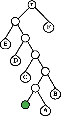
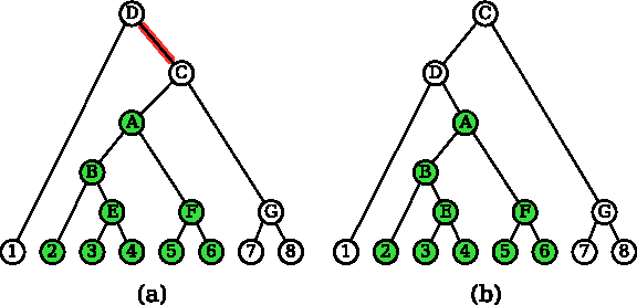
Consider for example the top-left chain tree in Figure 6a. Green (shaded) nodes are locked. Their lowest covering node is A (the root of the chain tree), but T(A) does not cover the locked nodes exactly. In the chain tree in Figure 6d, the node A covers locked nodes. A straightforward two-pass iterative grouping algorithm requiring \documentclass{aastex}\usepackage{amsbsy}\usepackage{amsfonts}\usepackage{amssymb}\usepackage{bm}\usepackage{mathrsfs}\usepackage{pifont}\usepackage{stmaryrd}\usepackage{textcomp}\usepackage{portland,xspace}\usepackage{amsmath,amsxtra}\pagestyle{empty}\DeclareMathSizes{10}{9}{7}{6} \begin{document} $${\cal O} ( h )$$\end{document} time (where h is the height of the regrouped tree) and \documentclass{aastex}\usepackage{amsbsy}\usepackage{amsfonts}\usepackage{amssymb}\usepackage{bm}\usepackage{mathrsfs}\usepackage{pifont}\usepackage{stmaryrd}\usepackage{textcomp}\usepackage{portland,xspace}\usepackage{amsmath,amsxtra}\pagestyle{empty}\DeclareMathSizes{10}{9}{7}{6} \begin{document} $${\cal O} ( 1 )$$\end{document} space is described in the remainder of this section.

FIG. 6.

Example of grouping. (a) Initially N = D. \documentclass{aastex}\usepackage{amsbsy}\usepackage{amsfonts}\usepackage{amssymb}\usepackage{bm}\usepackage{mathrsfs}\usepackage{pifont}\usepackage{stmaryrd}\usepackage{textcomp}\usepackage{portland,xspace}\usepackage{amsmath,amsxtra}\pagestyle{empty}\DeclareMathSizes{10}{9}{7}{6} \begin{document} $$6 \notin T ( 2 )$$\end{document} , \documentclass{aastex}\usepackage{amsbsy}\usepackage{amsfonts}\usepackage{amssymb}\usepackage{bm}\usepackage{mathrsfs}\usepackage{pifont}\usepackage{stmaryrd}\usepackage{textcomp}\usepackage{portland,xspace}\usepackage{amsmath,amsxtra}\pagestyle{empty}\DeclareMathSizes{10}{9}{7}{6} \begin{document} $$2 \in T ( 2 )$$\end{document} and D = l(B). S_r(D) is applied. (b) N = D, \documentclass{aastex}\usepackage{amsbsy}\usepackage{amsfonts}\usepackage{amssymb}\usepackage{bm}\usepackage{mathrsfs}\usepackage{pifont}\usepackage{stmaryrd}\usepackage{textcomp}\usepackage{portland,xspace}\usepackage{amsmath,amsxtra}\pagestyle{empty}\DeclareMathSizes{10}{9}{7}{6} \begin{document} $$6 \notin T ( B )$$\end{document} , \documentclass{aastex}\usepackage{amsbsy}\usepackage{amsfonts}\usepackage{amssymb}\usepackage{bm}\usepackage{mathrsfs}\usepackage{pifont}\usepackage{stmaryrd}\usepackage{textcomp}\usepackage{portland,xspace}\usepackage{amsmath,amsxtra}\pagestyle{empty}\DeclareMathSizes{10}{9}{7}{6} \begin{document} $$2 \in T ( B )$$\end{document} and D = l(A). S_τ(D) is applied. (c) N = D. \documentclass{aastex}\usepackage{amsbsy}\usepackage{amsfonts}\usepackage{amssymb}\usepackage{bm}\usepackage{mathrsfs}\usepackage{pifont}\usepackage{stmaryrd}\usepackage{textcomp}\usepackage{portland,xspace}\usepackage{amsmath,amsxtra}\pagestyle{empty}\DeclareMathSizes{10}{9}{7}{6} \begin{document} $$6 \in T ( A )$$\end{document} , and 2 is the leftmost leaf of T(A). First phase completed. N = F. \documentclass{aastex}\usepackage{amsbsy}\usepackage{amsfonts}\usepackage{amssymb}\usepackage{bm}\usepackage{mathrsfs}\usepackage{pifont}\usepackage{stmaryrd}\usepackage{textcomp}\usepackage{portland,xspace}\usepackage{amsmath,amsxtra}\pagestyle{empty}\DeclareMathSizes{10}{9}{7}{6} \begin{document} $$2 \notin T ( 5 )$$\end{document} and \documentclass{aastex}\usepackage{amsbsy}\usepackage{amsfonts}\usepackage{amssymb}\usepackage{bm}\usepackage{mathrsfs}\usepackage{pifont}\usepackage{stmaryrd}\usepackage{textcomp}\usepackage{portland,xspace}\usepackage{amsmath,amsxtra}\pagestyle{empty}\DeclareMathSizes{10}{9}{7}{6} \begin{document} $$6 \notin T ( 5 )$$\end{document} . Hence N = C. \documentclass{aastex}\usepackage{amsbsy}\usepackage{amsfonts}\usepackage{amssymb}\usepackage{bm}\usepackage{mathrsfs}\usepackage{pifont}\usepackage{stmaryrd}\usepackage{textcomp}\usepackage{portland,xspace}\usepackage{amsmath,amsxtra}\pagestyle{empty}\DeclareMathSizes{10}{9}{7}{6} \begin{document} $$2 \notin T ( F )$$\end{document} , \documentclass{aastex}\usepackage{amsbsy}\usepackage{amsfonts}\usepackage{amssymb}\usepackage{bm}\usepackage{mathrsfs}\usepackage{pifont}\usepackage{stmaryrd}\usepackage{textcomp}\usepackage{portland,xspace}\usepackage{amsmath,amsxtra}\pagestyle{empty}\DeclareMathSizes{10}{9}{7}{6} \begin{document} $$6 \in T ( F )$$\end{document} and C = r(A). S_l(C) is applied. (d) N = C and T(A) has 2 as the leftmost leaf and 6 as the rightmost leaf.

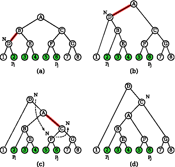
Consider a chain tree T and assume that it is the smallest subtree containing a locked sequence of leaves \documentclass{aastex}\usepackage{amsbsy}\usepackage{amsfonts}\usepackage{amssymb}\usepackage{bm}\usepackage{mathrsfs}\usepackage{pifont}\usepackage{stmaryrd}\usepackage{textcomp}\usepackage{portland,xspace}\usepackage{amsmath,amsxtra}\pagestyle{empty}\DeclareMathSizes{10}{9}{7}{6} \begin{document} $$L_{ij} = \{L_i , L_{i + 1} , \ldots , L_{j - 1}\} $$\end{document} , 1 ≤ i < j < n. T has to be grouped so that one node covers L_ij exactly. Let S_l(N) (respectively S_r(N)) denote the left (respectively, right) swap2 of the branch between node N and its parent. This is permissible only if N is a right (respectively, left) child (Fig. 5). The reader is referred to Cormen et al. (2009) for more on binary search trees and swaps.

FIG. 5.

Left and right swaps.

Consider the following iterative procedure beginning at the leaf L_i:

N = p(L_i)

while \documentclass{aastex}\usepackage{amsbsy}\usepackage{amsfonts}\usepackage{amssymb}\usepackage{bm}\usepackage{mathrsfs}\usepackage{pifont}\usepackage{stmaryrd}\usepackage{textcomp}\usepackage{portland,xspace}\usepackage{amsmath,amsxtra}\pagestyle{empty}\DeclareMathSizes{10}{9}{7}{6} \begin{document} $$L_{j - 1} \notin T ( r ( N ) )$$\end{document} do

if \documentclass{aastex}\usepackage{amsbsy}\usepackage{amsfonts}\usepackage{amssymb}\usepackage{bm}\usepackage{mathrsfs}\usepackage{pifont}\usepackage{stmaryrd}\usepackage{textcomp}\usepackage{portland,xspace}\usepackage{amsmath,amsxtra}\pagestyle{empty}\DeclareMathSizes{10}{9}{7}{6} \begin{document} $$L_i \in T ( r ( N ) )$$\end{document}

if N = r(p(N)) then S_l(N) else S_r(N)

else N = p(N).

At each iteration, the depth of the node N either reduces by 1 or it remains unchanged. In the latter case, the next iteration reduces the depth of N by 1. As a consequence, N will after a finite number of iterations cover L_ij. It is also obvious that L_i remains the leftmost leaf of T(N).

If T(N) exactly covers L_ij, the sought grouping is obtained. Assume therefore that L_j₋₁ is not the rightmost leaf of T(N).

Let N now denote the parent of L_j₋₁. The iterative procedure needed to make L_ij exactly covered is very similar to the one that resulted in N to become the root of the subtree having L_i as a leftmost leaf and being the lowest common ancestor of both L_i and L_j₋₁. The details are therefore omitted.

The discussion in this section can be summarized as follows:

Corollary 1

A chain tree with k locked leaves can be regrouped in \documentclass{aastex}\usepackage{amsbsy}\usepackage{amsfonts}\usepackage{amssymb}\usepackage{bm}\usepackage{mathrsfs}\usepackage{pifont}\usepackage{stmaryrd}\usepackage{textcomp}\usepackage{portland,xspace}\usepackage{amsmath,amsxtra}\pagestyle{empty}\DeclareMathSizes{10}{9}{7}{6} \begin{document} $${ \cal O} ( 1 )$$\end{document} space and \documentclass{aastex}\usepackage{amsbsy}\usepackage{amsfonts}\usepackage{amssymb}\usepackage{bm}\usepackage{mathrsfs}\usepackage{pifont}\usepackage{stmaryrd}\usepackage{textcomp}\usepackage{portland,xspace}\usepackage{amsmath,amsxtra}\pagestyle{empty}\DeclareMathSizes{10}{9}{7}{6} \begin{document} $${ \cal O} ( h )$$\end{document} time where h is the height of the chain tree. If the chain tree is balanced, then \documentclass{aastex}\usepackage{amsbsy}\usepackage{amsfonts}\usepackage{amssymb}\usepackage{bm}\usepackage{mathrsfs}\usepackage{pifont}\usepackage{stmaryrd}\usepackage{textcomp}\usepackage{portland,xspace}\usepackage{amsmath,amsxtra}\pagestyle{empty}\DeclareMathSizes{10}{9}{7}{6} \begin{document} $$h \in { \cal O} ( \log n )$$\end{document} where n is the number of leaves.

6. Rebalancing

When locking and grouping chain trees, they will inevitably become unbalanced in the sense that the heights of the siblings may differ by more than one. There are in fact two types of unbalance that can occur. The less important unbalance may occur in exactly covering trees that emerge after regrouping. This is not so important because bonds of leaves covered by such subtrees will normally not be rotated. But this unbalance after regrouping can still have undesirable influence on clash detection.

The second type of unbalance occurs when regrouped, exactly covering subtrees are considered as leaf nodes (represented by their roots) Since bounding volumes associated with nodes of such subtrees and, in particular, with their roots can be expected to remain unchanged in subsequent iterations, they can be computed by more precise, slower methods. Search for clashes through such subtrees will therefore occur less often because of tighter bounding volumes. Such subtrees can therefore be pushed further away from the root of the chain tree. Futhermore, this will bring some unlocked leaves closer to the root making the rotations and clash detections less expensive. An example of rebalancing can be seen in Figure 7.

FIG. 7.

Rebalancing the chain tree. (a) Left child of the root has height 0 while right child has height 2 (subtree rooted at A is locked and therefore regarded as a leaf). (b) Left swap on the branch from C to D results in a tree where both children of the root have height 1.

Suppose that a chain tree contains an internal node A of height k, k ≥ 3. Let B = l(A), C = r(A), D = l(B), and E = r(B). Suppose that h(B) = k − 1 and h(C) ≤ k − 3. The case h(B) ≤ k − 3 and h(C) = k − 1 is dealt with in analogous manner (right swaps being replaced by left swaps). Assume furthermore that no other pair of siblings in T(A) has heights differing by 2 or more.

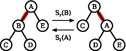
Suppose first that h(D) = k − 2 and k − 3 ≤ h(E) ≤ k − 2 (Fig. 8a). Perform the right swap on the branch between B and A. As a consequence, B becomes the root of the subtree, A becomes the right child of B, D becomes the left child of B, while E becomes the left child of A as shown in Figure 8a. If h(E) − h(C) > 1, rebalance A again. Notice however that the height of A is at least one less than before the swap. 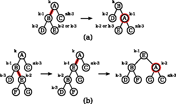Hence, rebalancing of A may propagate down the chain tree but cannot be repeated more than \documentclass{aastex}\usepackage{amsbsy}\usepackage{amsfonts}\usepackage{amssymb}\usepackage{bm}\usepackage{mathrsfs}\usepackage{pifont}\usepackage{stmaryrd}\usepackage{textcomp}\usepackage{portland,xspace}\usepackage{amsmath,amsxtra}\pagestyle{empty}\DeclareMathSizes{10}{9}{7}{6} \begin{document} $${ \cal O} ( k )$$\end{document} times, and k is bounded by the height of the chain tree.

FIG. 8.

The two rebalancing cases considered in the rebalancing method. The method ensures that unbalanced nodes are either balanced or propagated downwards in the tree.

Suppose next that h(D) = k − 3 and h(E) = k − 2 (Fig. 8b). Let F = l(E) and G = r(E). Perform the left swap on the branch from E to B (making E the left child of A) followed by the right swap on the branch from E to A. E becomes the root of the subtree. A becomes the right child of E with G being its left child and C being its right child, as shown in Figure 8b. If h(G) − h(C) > 1, rebalance A again. Also in this case, the rebalancing of A can propagate down the chain but cannot be repeated ore than \documentclass{aastex}\usepackage{amsbsy}\usepackage{amsfonts}\usepackage{amssymb}\usepackage{bm}\usepackage{mathrsfs}\usepackage{pifont}\usepackage{stmaryrd}\usepackage{textcomp}\usepackage{portland,xspace}\usepackage{amsmath,amsxtra}\pagestyle{empty}\DeclareMathSizes{10}{9}{7}{6} \begin{document} $${ \cal O} ( k )$$\end{document} times.

The above procedure explains how to perform a rebalancing step given the node A. The rebalancing of the entire chain tree is performed by applying this step to every single node in the chain tree in a bottom-up fashion as a preprocessing step. If, for example, α-helices and β-strands have been formed, their bonds are locked and the chain tree is regrouped so that all secondary structures are covered exactly. Next, subtrees exactly covering secondary structures are replaced by their roots. The chain tree is rebalanced (identifying siblings with height difference of more than 1 in a bottom-up fashion). Finally, the subtrees exactly covering secondary structures are added back to the chain tree. The chain tree of the protein 1CTFA (see Fig. 12 below) before and after locking, grouping, and rebalancing is shown in Figure 9. The chain tree was also rearranged so that peptide planes are exactly covered in the bottom chain tree (subtrees of height 2 have 3 instead of four leaves).

FIG. 9.

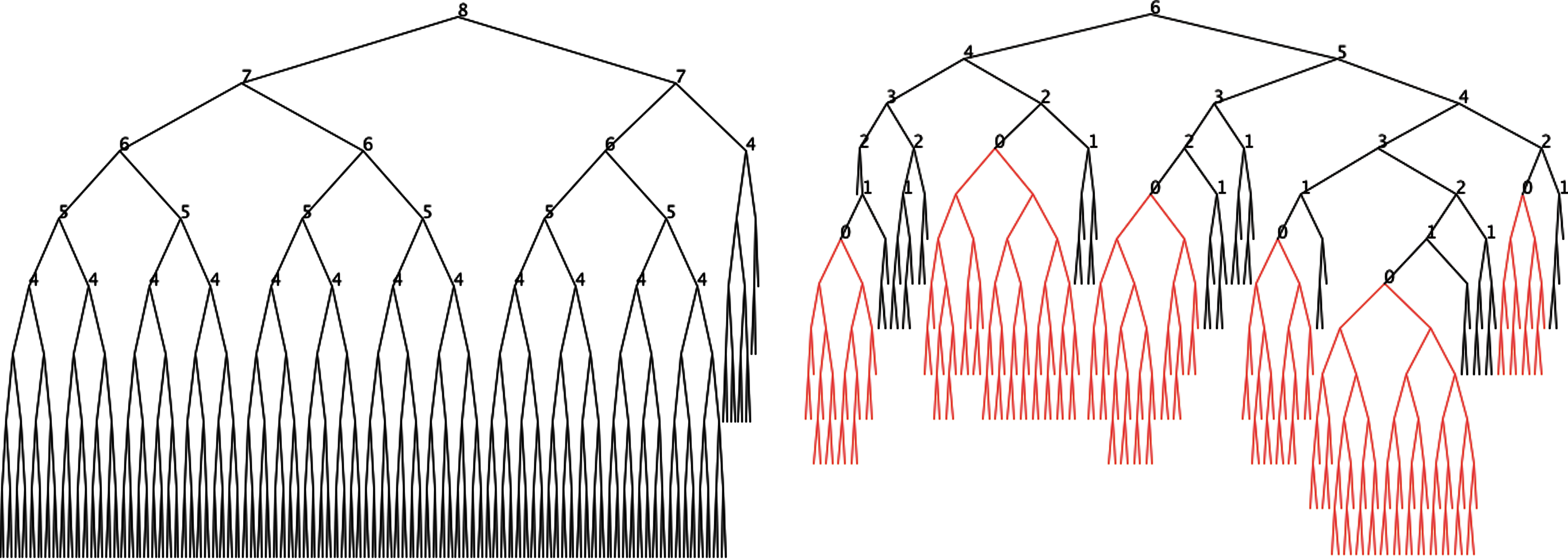
The chain tree of 1CTFA before and after locking and rebalancing. Red/shaded subtrees are locked subtrees of secondary structures. Integers at nodes are their heights. Note that during the rebalancing the roots of red/shaded subtrees and roots of peptide planes are regarded as leaves of height 0.

The discussion in this section can be summarized as follows:

Corollary 2

Rebalancing of a single node in the chain tree can be done in \documentclass{aastex}\usepackage{amsbsy}\usepackage{amsfonts}\usepackage{amssymb}\usepackage{bm}\usepackage{mathrsfs}\usepackage{pifont}\usepackage{stmaryrd}\usepackage{textcomp}\usepackage{portland,xspace}\usepackage{amsmath,amsxtra}\pagestyle{empty}\DeclareMathSizes{10}{9}{7}{6} \begin{document} $${ \cal O} ( 1 )$$\end{document} space and \documentclass{aastex}\usepackage{amsbsy}\usepackage{amsfonts}\usepackage{amssymb}\usepackage{bm}\usepackage{mathrsfs}\usepackage{pifont}\usepackage{stmaryrd}\usepackage{textcomp}\usepackage{portland,xspace}\usepackage{amsmath,amsxtra}\pagestyle{empty}\DeclareMathSizes{10}{9}{7}{6} \begin{document} $${ \cal O} ( h )$$\end{document} time where h is the height of the node. If the chain tree is balanced, then \documentclass{aastex}\usepackage{amsbsy}\usepackage{amsfonts}\usepackage{amssymb}\usepackage{bm}\usepackage{mathrsfs}\usepackage{pifont}\usepackage{stmaryrd}\usepackage{textcomp}\usepackage{portland,xspace}\usepackage{amsmath,amsxtra}\pagestyle{empty}\DeclareMathSizes{10}{9}{7}{6} \begin{document} $$h \in { \cal O} ( \log n )$$\end{document} where n is the number of leaves. Rebalancing of all nodes in the chain tree (bottom-up) can then be carried out in \documentclass{aastex}\usepackage{amsbsy}\usepackage{amsfonts}\usepackage{amssymb}\usepackage{bm}\usepackage{mathrsfs}\usepackage{pifont}\usepackage{stmaryrd}\usepackage{textcomp}\usepackage{portland,xspace}\usepackage{amsmath,amsxtra}\pagestyle{empty}\DeclareMathSizes{10}{9}{7}{6} \begin{document} $${ \cal O} ( n \log n )$$\end{document} time.

7. Bounding Volumes

Use of bounding volumes in chain trees requires efficient methods to:

• transform a bounding volume to another coordinate system,

• decide if two bounding volumes intersect,

• find a tight volume bounding two smaller volumes,

• find a tight volume bounding a set of bonds or atoms.

In this study we decided to use line-segment swept spheres as bounding volumes. A line-segment swept sphere (LSS) is the Minkowski sum of an arbitrarily oriented line-segment and a sphere. A LSS is therefore fully specified by the two end-points of the line-segment and the radius of the sphere. A LSS is also sometimes referred to as a capsule, a capped cylinder, a spherocylinder (Ericson, 2005), or even as a cigar (Bereg, 2004).

Our choice was motivated by our intuition that LSSs are much better suited to bound proteins (especially if protein chains are appropriately divided into subchains) than oriented bounding boxes (Gottschalk and Manocha, 1996) and rectangular swept spheres (Larsen et al., 2000; Eberly, 2000) that are more commonly used. Our intuition proved in fact to be correct. The comparative study (Fonseca and Winter, 2010) of various bounding volumes clearly indicated that LSSs are superior (at least for protein chains). The relative speed-up is in fact greater when using either adjustable chain trees with oriented bounding boxes or rectangular swept spheres. In terms of dramatic speed-ups, LSSs are the least spectacular choice. But we nevertheless opted for LSSs, as they are most suitable for protein chains.

A LSS is transformed to another coordinate system by applying an appropriate transform matrix to the end-points of its defining line-segment.

The intersection test between two LSSs is performed as described in Ericson (2005). It basically reduces to deciding if the distance between the two defining line-segments is less than the sum of the radii.

To find a good (but not necessarily optimal) LSS bounding a set of points, the principal component, \documentclass{aastex}\usepackage{amsbsy}\usepackage{amsfonts}\usepackage{amssymb}\usepackage{bm}\usepackage{mathrsfs}\usepackage{pifont}\usepackage{stmaryrd}\usepackage{textcomp}\usepackage{portland,xspace}\usepackage{amsmath,amsxtra}\pagestyle{empty}\DeclareMathSizes{10}{9}{7}{6} \begin{document} $$\vec{d}$$\end{document} , of the points is used as the direction of the defining line-segment. The points are projected onto a plane normal to \documentclass{aastex}\usepackage{amsbsy}\usepackage{amsfonts}\usepackage{amssymb}\usepackage{bm}\usepackage{mathrsfs}\usepackage{pifont}\usepackage{stmaryrd}\usepackage{textcomp}\usepackage{portland,xspace}\usepackage{amsmath,amsxtra}\pagestyle{empty}\DeclareMathSizes{10}{9}{7}{6} \begin{document} $$\vec{d}$$\end{document} and the smallest enclosing circle C with radius r is found. C together with \documentclass{aastex}\usepackage{amsbsy}\usepackage{amsfonts}\usepackage{amssymb}\usepackage{bm}\usepackage{mathrsfs}\usepackage{pifont}\usepackage{stmaryrd}\usepackage{textcomp}\usepackage{portland,xspace}\usepackage{amsmath,amsxtra}\pagestyle{empty}\DeclareMathSizes{10}{9}{7}{6} \begin{document} $$\vec{d}$$\end{document} , defines an infinitely extended cylinder that contains all the points (now back in 3D). Finally, the infinite line-segment is capped with two hemispheres of radius r such that the points are bounded. Centers of these hemispheres define end-points of the defining line-segment.

To find a good (but not necessarily optimal) LSS, B bounding two smaller LSSs, B_l and B_r, the four spheres defined by the end-points of the line-segments of B_l and B_r and their radii are considered. The direction \documentclass{aastex}\usepackage{amsbsy}\usepackage{amsfonts}\usepackage{amssymb}\usepackage{bm}\usepackage{mathrsfs}\usepackage{pifont}\usepackage{stmaryrd}\usepackage{textcomp}\usepackage{portland,xspace}\usepackage{amsmath,amsxtra}\pagestyle{empty}\DeclareMathSizes{10}{9}{7}{6} \begin{document} $$\vec{d}$$\end{document} of B is determined as the direction between the two most remote points on the surfaces of these four spheres. The four spheres are projected onto a plane orthogonal to \documentclass{aastex}\usepackage{amsbsy}\usepackage{amsfonts}\usepackage{amssymb}\usepackage{bm}\usepackage{mathrsfs}\usepackage{pifont}\usepackage{stmaryrd}\usepackage{textcomp}\usepackage{portland,xspace}\usepackage{amsmath,amsxtra}\pagestyle{empty}\DeclareMathSizes{10}{9}{7}{6} \begin{document} $$\vec{d}$$\end{document} as four circles (one will be nested in another and can be disregarded). The smallest circle enclosing the remaining three circles together with \documentclass{aastex}\usepackage{amsbsy}\usepackage{amsfonts}\usepackage{amssymb}\usepackage{bm}\usepackage{mathrsfs}\usepackage{pifont}\usepackage{stmaryrd}\usepackage{textcomp}\usepackage{portland,xspace}\usepackage{amsmath,amsxtra}\pagestyle{empty}\DeclareMathSizes{10}{9}{7}{6} \begin{document} $$\vec{d}$$\end{document} , defines an infinitely extended cylinder containing all four spheres. Finally, the cylinder is capped as explained above.

8. Computational Results

The main purpose of adjustable chain trees is to deal with α-helices and β-strands (such secondary structures will normally be fixed beforehand or created early in the folding process). In order to justify the need for adjustable chain trees, it is therefore necessary to establish if occurrences of secondary structures are sufficiently common. We argue in Subsection 8.1 that this is indeed the case, and we choose a set of chains for computational experiments. In Subsection 8.2, we set up an appropriate cost measure to evaluate the speed-up independently of implementational and hardware details. In Subsection 8.3, we show to what extent adjustable chain trees speed-up clash detections.

8.1. Data sets

Statistics presented in this section are based on proteins (or rather chains) taken from PDBSelect 25 (Berman et al., 2000). The version we consider contains 4018 chains. Forty-two of these were filtered out because of various format problems.

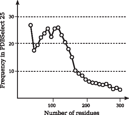
Lengths of chains in PDBSelect 25 are shown in Figure 10. Frequencies of chains with n residues, 10 × l ≤ n ≤ 10 × l + 9, \documentclass{aastex}\usepackage{amsbsy}\usepackage{amsfonts}\usepackage{amssymb}\usepackage{bm}\usepackage{mathrsfs}\usepackage{pifont}\usepackage{stmaryrd}\usepackage{textcomp}\usepackage{portland,xspace}\usepackage{amsmath,amsxtra}\pagestyle{empty}\DeclareMathSizes{10}{9}{7}{6} \begin{document} $$l = 0 , 1 , \ldots , 29$$\end{document} , are averaged. Chains with more than 300 residues are rare, and therefore not shown. It can be seen that chains with 110–119 residues are among the most common.

FIG. 10.

Distribution of lengths of chains in PDBSelect 25.

Figure 11 shows the distribution of chains in PDBSelect 25 with respect to the portion of residues in secondary structures. Out of the 3976 considered chains, only 60 had no secondary structures. More than 75% of all chains had over 50% of their residues in either helices or β-strands.

FIG. 11.

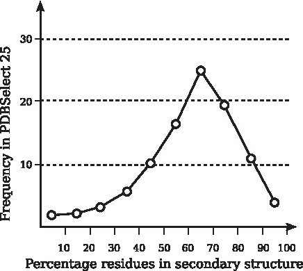
Percentage of secondary structures in chains of PDBSelect 25.

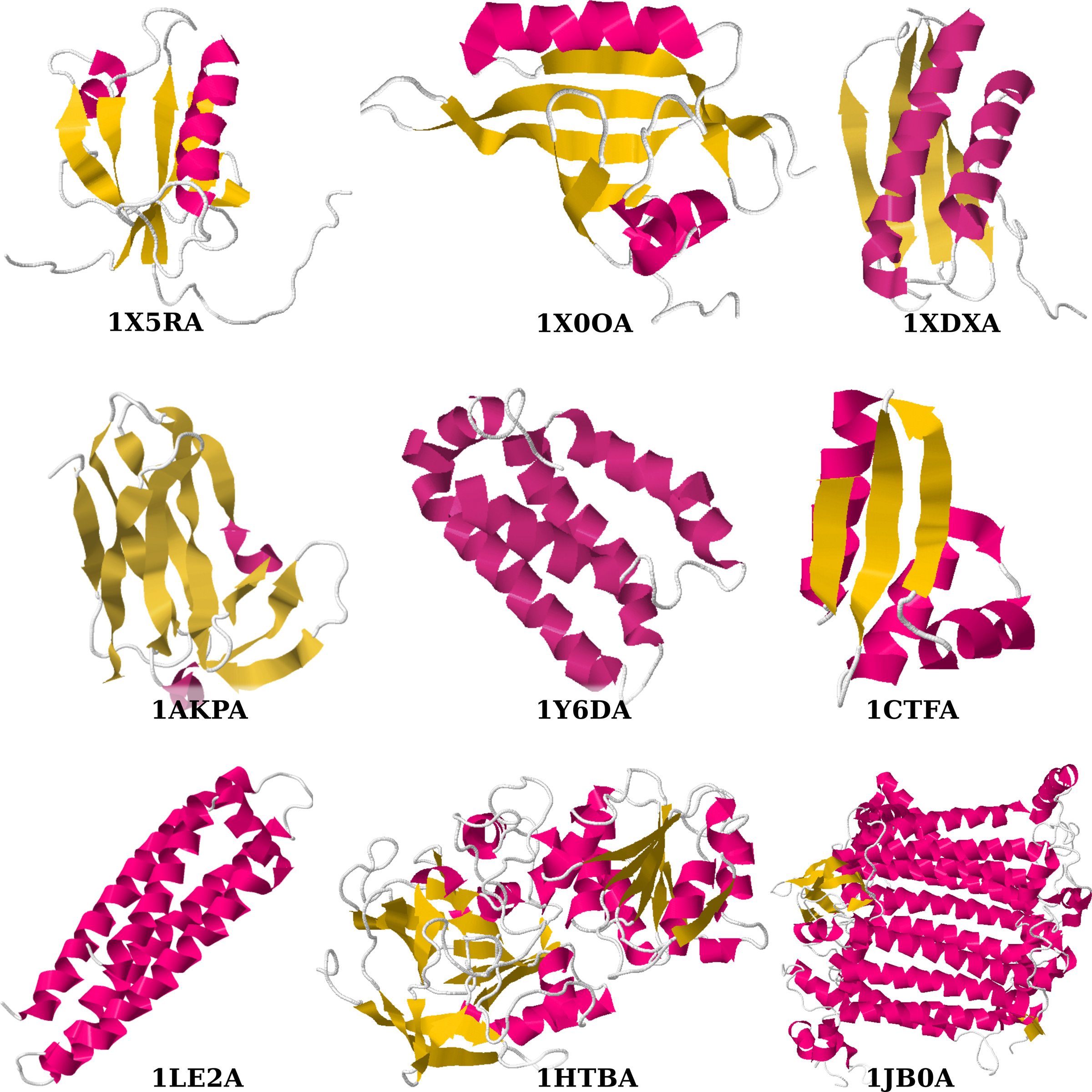
Based on the above statistics, chain tree experiments were performed on two data sets. The first data set had five chains with 110–119 residues, the typical length in PDBSelect 25. These five chains were selected so that the portions of residues in secondary structures were one in each of the five intervals \documentclass{aastex}\usepackage{amsbsy}\usepackage{amsfonts}\usepackage{amssymb}\usepackage{bm}\usepackage{mathrsfs}\usepackage{pifont}\usepackage{stmaryrd}\usepackage{textcomp}\usepackage{portland,xspace}\usepackage{amsmath,amsxtra}\pagestyle{empty}\DeclareMathSizes{10}{9}{7}{6} \begin{document} $$[ i \times 10 \% , ( i + 1 ) \times 10 \% [ , i = 4 , 5 , \ldots , 8$$\end{document} . The first five rows of Table 1 provide some basic characteristics of the five chosen chains.

Table 1.

Second Column is the Number of Residues in the Examined Chains

PDB-id	No. of res.	% in αβ	#α + #β
1X5RA	112	42%	2 + 6
1X0OA	119	58%	3 + 5
1XDXA	114	63%	2 + 4
1AKPA	114	79%	2 + 11
1Y6DA	114	82%	7 + 0
1CTFA	68	82%	3 + 3
1LE2A	144	83%	5 + 0
1HTBA	374	52%	10 + 19
1JB0A	755	62%	12 + 4

The third column indicates the portion of residues in secondary structures. The fourth column indicates the number of α-helices and β-strands.

The second data set is the four chains used in the seminal article on chain trees (Lotan et al., 2004). The lengths vary from 68 to 755 residues. The last four rows of Table 1 indicate which chains are in the second data set. Figure 12 shows all nine examined chains.

FIG. 12.

Chains in the two data sets displayed using Jmol (JMol, 2010). The first five chains have almost the same length, but different distributions of secondary structures. The last four chains are from Lotan et al. (2004) and have varying lengths.

8.2. Cost measure

To evaluate how much grouping of peptide planes, locking, regrouping, and balancing improves the efficiency of chain trees, we determined the average cost of a single rotation in the chain tree. The cost of a rotation was defined as \documentclass{aastex}\usepackage{amsbsy}\usepackage{amsfonts}\usepackage{amssymb}\usepackage{bm}\usepackage{mathrsfs}\usepackage{pifont}\usepackage{stmaryrd}\usepackage{textcomp}\usepackage{portland,xspace}\usepackage{amsmath,amsxtra}\pagestyle{empty}\DeclareMathSizes{10}{9}{7}{6} \begin{document} \begin{align*}N_V C_V + N_U C_U + N_P C_P\end{align*}\end{document}

where

• N_V is the number of bounding volume pairs tested for overlap,

• C_V is the cost of testing two bounding volumes for overlap,

• N_U is the number of bounding volumes updated due to rotations,

• C_U is the cost of updating a bounding volume,

• N_P is the number of primitive pairs (bonds) tested for overlap,

• C_P is the cost of testing a primitive pair for overlap.

The three costs—C_V , C_U, and C_P—shown in Table 2 were determined experimentally. Using the chain tree, a 1° rotation of every non-locked bond (all peptide bonds and all bonds in secondary structures were locked) was carried out. The subsequent clash detection typically involved many volume intersection tests. C_V was determined by measuring the avarage CPU-time for all the resulting volume intersection tests (no matter their outcome). The transformation of one bounding volume into the coordinate system of another bounding volume was included in C_V. Rotations that did not result in clashes were used to update the chain tree. Such an update requires updating of all bounding volumes associated with nodes between the rotated bond and the root of the chain tree. C_U was determined by measuring the average CPU-time of all such bounding volume updates. The transformation of the bounding volume of the right subtree to the coordinate system of the bounding volume of the left subtree was included in C_U. To increase the accuracy of C_V and C_U, they were averaged over 100 repetitions.

Table 2.

Average Costs (in ms) of Checking LSSs for Overlap (C_V ), Updating an LSS (C_U), and Checking Primitives for Overlap C_P

C_V	C_U	C_P
0.00075	0.0020	0.00040

Testing a pair of primitives corresponds to finding the distance between two atoms. To determine C_P , we therefore generated 10⁶ random point-pairs and measured the average time it took to transform one point to another point's coordinate system, and then to find their distance.

8.3. To adjust or not to adjust

In the experiments reported in this subsection, all peptide bonds were locked. The φ torsion angle on the first N-C_α bond and the ψ torsion angle on the last C_α-C bond do not affect the structures of chains, so the corresponding bonds were also locked.

Three sets of experiments were carried out. In the first set, chain trees were set up to represent native structures of the selected chains. The coordinates of all atoms were obtained from the Protein Data Bank (PDB) (Berman et al., 2000). Ten rotations by the angles ±i × 4°, \documentclass{aastex}\usepackage{amsbsy}\usepackage{amsfonts}\usepackage{amssymb}\usepackage{bm}\usepackage{mathrsfs}\usepackage{pifont}\usepackage{stmaryrd}\usepackage{textcomp}\usepackage{portland,xspace}\usepackage{amsmath,amsxtra}\pagestyle{empty}\DeclareMathSizes{10}{9}{7}{6} \begin{document} $$i = 1 , 2 , \ldots , 5$$\end{document} , were applied to each unlocked bond. For each selected chain, six types of chain trees were examined: unlocked or locked peptide plane, unlocked or locked (and regrouped) secondary structures, and unbalances or balanced secondary structures (only in case of regrouping).

The average costs of the first set of experiments (rotations applied to the native structures) are shown in Table 3. It is clear that grouping peptide planes, locking, grouping and balancing secondary structures provides a substantial speed-up. Also, not surprisingly, the cost improvements tend to increase for chains with high fraction of secondary structures.

Table 3.

Average Costs (in ms) of Rotations of Native Structures

Native	1X5RA	1X0OA	1XDXA	1AKPA	1Y6DA
All rotations
—	0.291	0.283	0.234	0.234	0.251
P	0.226	0.197	0.164	0.213	0.164
S	0.245	0.233	0.170	0.204	0.113
PS	0.208	0.200	0.155	0.183	0.099
SB	0.243	0.256	0.184	0.217	0.095
PSB	0.200	0.194	0.141	0.188	0.091

Clashing rotations only
Ratio	33.3%	19.1%	29.4%	36.2%	15.6%
—	0.296	0.202	0.185	0.214	0.323
P	0.209	0.165	0.148	0.180	0.134
S	0.258	0.184	0.142	0.204	0.170
PS	0.204	0.163	0.127	0.160	0.122
SB	0.260	0.203	0.160	0.178	0.131
PSB	0.194	0.164	0.120	0.164	0.099

Non-clashing rotations only
Ratio	66.7%	80.9%	70.6%	63.8%	84.4%
—	0.288	0.309	0.257	0.244	0.242
P	0.235	0.203	0.178	0.234	0.170
S	0.239	0.248	0.182	0.204	0.109
PS	0.211	0.210	0.166	0.196	0.095
SB	0.235	0.272	0.195	0.235	0.092
PSB	0.203	0.201	0.149	0.201	0.089

The three-character code in the first column indicates which improvements were applied to the chain tree. A “P” indicates that peptide planes were grouped. The “S” indicates that secondary structures were locked and the chain tree was regrouped. Finally, a “B” indicates that the chain tree was rebalanced (only applicable with “S”). The fastest configuration is highlighted in boldface for each protein.

The second section in Table 3 shows the average costs of clashing rotations, while the third section shows the average costs of non-clashing rotations. Ratios of clashing and non-clashing rotations are also provided. Figure 13 summarizes graphically the results of Table 3.

FIG. 13.

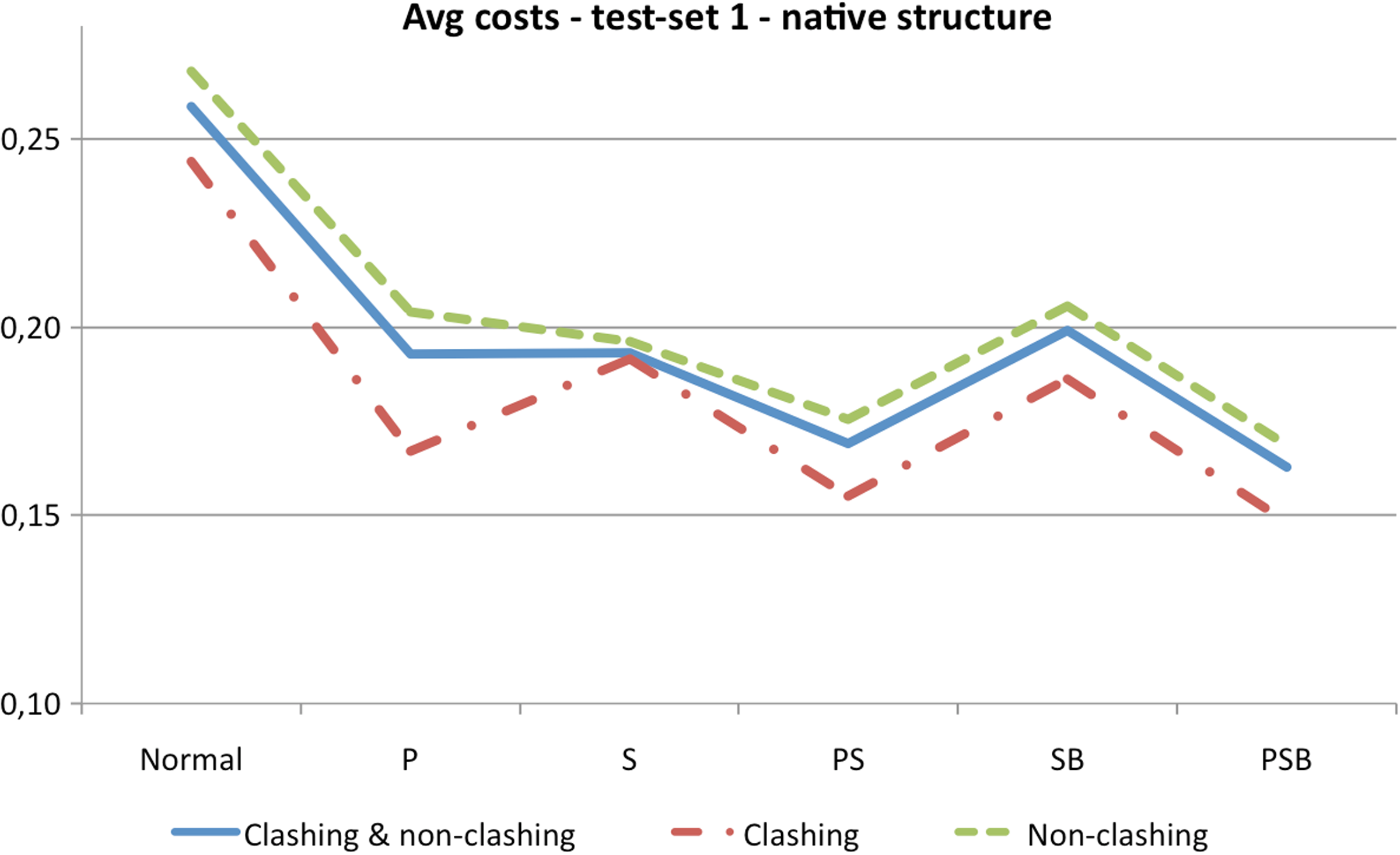
Summary of Table 3. The costs are averaged over all five chains. “P” indicates that peptide planes were grouped, “S” that secondary structures were locked and grouped, and “B” that chain trees were rebalanced.

In the second set of experiments, adjustable chain trees were used on structures not as tight packed as was the case for native structures. This is a very typical situation during the folding process. These loosely packed structures were obtained as follows. Their initial conformation were unfolded structures: all φ and ψ angles were set to 180°. ω-angles of peptide bonds were extracted from the PDB. Non-clashing rotations that minimized the RMSD between the current and the native conformation were applied as long as the RMSD was above 10Å. Then, 10 rotations by the angles ±i × 4°, \documentclass{aastex}\usepackage{amsbsy}\usepackage{amsfonts}\usepackage{amssymb}\usepackage{bm}\usepackage{mathrsfs}\usepackage{pifont}\usepackage{stmaryrd}\usepackage{textcomp}\usepackage{portland,xspace}\usepackage{amsmath,amsxtra}\pagestyle{empty}\DeclareMathSizes{10}{9}{7}{6} \begin{document} $$i = 1 , 2 , \ldots , 5$$\end{document} , were applied to each unlocked bond. Table 4 shows the average rotation costs analogous to the results for native structures shown in Table 3. Once again, substantial speed-up can be observed when peptide planes are grouped and when secondary structures are locked, regrouped, and rebalanced. This applies equally well for clashing and non-clashing rotations. Figure 14 summarizes graphically the results of Table 4.

FIG. 14.

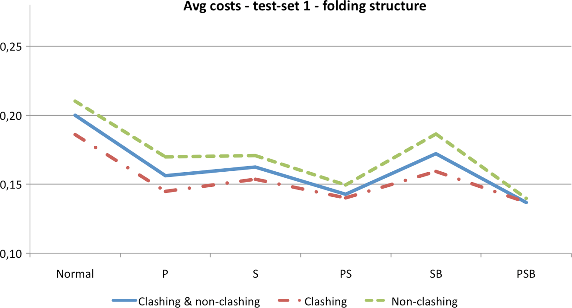
Summary of Table 4. The costs are averaged over all five chains. “P” indicates that peptide planes were grouped, “S” that secondary structures were locked and grouped, and “B” that chain trees were rebalanced.

Table 4.

Average Costs (in ms) of Rotations of Folding Structures

Folding RMSD	1X5RA 10.0Å	1X0OA 10.0Å	1XDXA 10.0Å	1AKPA 10.0Å	1Y6DA 10.0Å
All rotations
—	0.223	0.241	0.158	0.231	0.147
P	0.173	0.175	0.137	0.193	0.102
S	0.190	0.206	0.122	0.184	0.110
PS	0.173	0.161	0.109	0.172	0.098
SB	0.202	0.212	0.137	0.200	0.110
PSB	0.162	0.152	0.105	0.179	0.086

Clashing rotations
Ratio	37.4%	31.1%	43.0%	68.2%	17.5%
—	0.219	0.185	0.147	0.241	0.138
P	0.173	0.138	0.135	0.176	0.102
S	0.196	0.152	0.118	0.192	0.110
PS	0.183	0.121	0.110	0.164	0.123
SB	0.213	0.153	0.136	0.192	0.103
PSB	0.171	0.130	0.107	0.171	0.106

Non-clashing rotations
Ratio	62.6%	68.9%	57.0%	31.8%	82.5%
—	0.225	0.295	0.170	0.212	0.149
P	0.173	0.199	0.140	0.236	0.101
S	0.186	0.266	0.127	0.164	0.110
PS	0.168	0.192	0.108	0.185	0.094
SB	0.195	0.277	0.137	0.211	0.112
PSB	0.157	0.162	0.104	0.194	0.082

“P” indicates that peptide planes were grouped, “S” that secondary structures were locked and grouped, and “B” that chain trees were rebalanced. The fastest configuration is highlighted in boldface for each protein.

In the first and second sets of experiments, adjustable chain trees were intentionally tested on chains with comparable number of residues but with various fractions of secondary structures. But the usability of adjustable chain trees should increase as the number of residues in chains increases. In order to show this, we tested adjustable chain trees on four chains used by Lotan et al. (2004). These were 1CTFA (68 residues), 1LE2A (144 residues), 1HTBA (374 residues), and 1JB0A (755 residues).

The performance of adjustable chain trees was tested in a slightly different way than in the previous two sets of experiments, since non-clashing rotations become rare for longer chains already when the RMSD is around 30Å. If a rotation did not result in a clash and the RMSD between current and native conformation was reduced, then the next rotation was applied to the improved conformation. If the RMSD did not decrease or if the rotation resulted in a clash, the new conformation was rejected and the next rotation was applied to the old conformation. The rotations were applied until 100 consecutive rotations did not give any RMSD improvement. Structures obtained in this manner were not as tightly packed as the native structures. Hence, they can be considered as realistic structures somewhere in the middle of the folding process. Average costs of rotations in native and folding structures are reported in Table 5. Once again, a dramatic improvement can be observed. But it seems that it is not dependent on the number of residues but rather on the size of the fractions of secondary structures. Figure 15 summarizes graphically the results of Table 5.

FIG. 15.

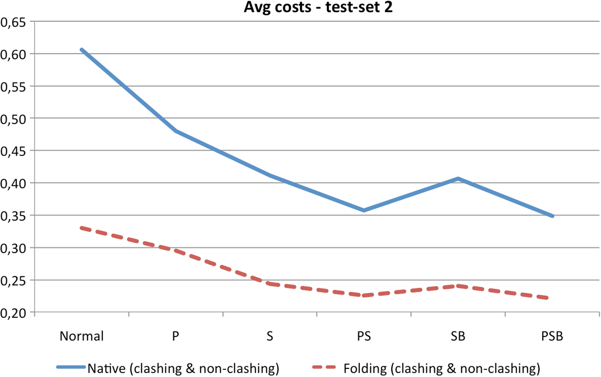
Summary of Table 5. The costs are averaged over all four proteins. “P” indicates that peptide planes were grouped, “S” that secondary structures were locked and grouped, and “B” that chain trees were rebalanced.

Table 5.

Average Costs (in ms) of Rotations of Structures from Lotan et al. (2004)

Native
PDB-id	1CTFA	1LE2A	1HTBA	1JB0A
—	0.177	0.311	0.961	0.975
P	0.142	0.257	0.712	0.810
S	0.124	0.101	0.785	0.634
PS	0.101	0.113	0.605	0.608
SB	0.119	0.118	0.754	0.634
PSB	0.087	0.113	0.601	0.593

Folding
RMSD	10.9Å	6.3Å	28.9Å	35.2Å
—	0.102	0.236	0.407	0.575
P	0.091	0.274	0.324	0.491
S	0.076	0.103	0.363	0.431
PS	0.082	0.123	0.301	0.394
SB	0.080	0.127	0.368	0.385
PSB	0.085	0.141	0.299	0.358

It should be expected that the addition of side chains will reduce the speed-up obtained by using adjustable chain trees rather than standard chain trees. Neither α-helices nor β-strands with side chains can be bounded as tight. Although our implementation has not yet been extended to include side chains, we investigated the speed-up of adjustable chain trees when all bounding volumes had an added radius of 2Å, 4Å, and 6Å. Bounding volumes will then contain larger and larger portions of side chains. While the speed-up becomes less dramatic as the radius increases, it is still advantageous to use adjustable chain trees (results are not included here).

Blowing up the radii of all atoms is of course a very primitive approach. Once side chains can be bounded by their own tighter bounding volumes, the advantage of using adjustable chain trees will be restored (although it will never be as good as when side chains are ignored). In some applications, non-clashing conformations of the backbone are generated first and appropriate rotamers are added afterwards. The use of adjustable chain trees rather than standard chain trees is then an obvious choice.

9. Conclusion

In this article, we suggested a modification of chain trees particularly suitable for the detection of clashes in folding simulations or structure predictions of the backbone of protein chains. As α-helices and β-strands are either predicted beforehand or are created relatively early in the folding or prediction process, locking, rearranging, and rebalancing can be done in a preprocessing phase. Rearrangement of secondary structures and peptide planes results in chain trees with much tighter bounding volumes. Our results clearly indicate that adjustable chain trees provide a substantial speed-up in the detection of clashes and in the update of conformations.

We investigated elsewhere (Fonseca and Winter, 2010) how adjustable chain trees perform when other bounding volumes—such as spheres, capsules, and rectangular swept spheres—are used. Similar speed-ups were observed for all these bounding volumes when switching from the ordinary chain tree to the adjustable version.

Adjustable chain trees can also be used for the efficient determination of free energy changes when moving from one conformation to another. Bounding volumes will in this context typically have larger volumes, and more clash checks will be required. This is not only due to the increased volumes, but also to the fact that the entire chain tree has to be checked for overlaps. We believe that adjustable chain trees will prove just as useful in energy calculations as they did in clash detection.

Footnotes

Acknowledgment

We would like to thank Kevin Karplus for valuable comments and suggestions during the preparation of this manuscript.

Disclosure Statement

No competing financial interests exist.

1

The term “search” is included to indicate the implicit ordering of subchains represented by the nodes: the subchain of the left child of a node directly precedes the subchain of its right child.

2

Swaps are in the binary search tree literature called “rotations”, but we wish to avoid confusion with bond rotations.

References

Berman

H.M.

, Westbrook

, Feng

et al. 2000. The Protein Data Bank. Nucleic Acids Res., 28:235–242. www.pdb.org. 2011 February 1.

Bereg

2004. Cylindrical hierarchy for deforming necklaces. Int. J. Comput. Geom. Appl., 14:3–17.

Branden

, Tooze

1999. Introduction to Protein Structure, 2nd. Garland Publishing: New York.

Cormen

T.H.

, Leiserson

C.E.

, Rivest

et al. 2009. Introduction to Algorithms, 3rd. MIT Press: Cambridge, MA.

Eberly

D.H.

2000. 3D Game Engine Design: A Practical Approach to Real-Time Computer Graphics. Morgan Kaufmann: New York.

Ericson

2005. Real-Time Collision Detection. Elsevier: New York.

Fonseca

, Winter

2010. Bounding volumes for proteins—a comparative study [Technical Report] Department of Computer Science, University of Copenhagen: Denmark.

Gottschalk

, Lin

, Manocha

1996. OBB-Tree: a hierarchical structure for rapid interference detection. Proc. 23rd Annu. Conf. Comput. Graphics Interactive Techniq., 171–180.

JMol. 2010. JMol: an open-source Java viewer for chemical structures in 3D. www.jmol.org. 2011 February 1.

10.

Kolodny

, Guibas

, Levitt

et al. 2005. Inverse kinematics in biology: the protein loop closure problem. Int. J. Robot. Res., 24:151–163.

11.

Larsen

, Gottschalk

, Lin

M.C.

et al. 2000. Fast distance queries with rectangular swept sphere volumes. Proc. IEEE Conf. Robot. Automation, 4:3719–3726.

12.

Lotan

, Schwarzer

, Halperin

et al. 2004. Algorithm and data structures for efficient energy maintenance during Monte Carlo simulation of proteins. J. Comput. Biol., 11:902–932.

13.

Wikipedia. 2010. File:Ramachandran plot general 100K.jpg. http://en.wikipedia.org/wiki/File:Ramachandran_plot_general_100K.jpg. 2011 February 1

Lovell

S.C.

Davis

I.W.

, Arendall

W.B.

III

et al. Structure validation by Cα geometry: φ, ψ and Cβ deviation: Proteins, Structure, Function, and Bioinformatics. 50,3:437–450 February 15, 2003.