Tracing the Most Parsimonious Indel History

Abstract

Sequence alignment (the grouping of homologous bases into one column) is fundamental to almost any task in comparative genomics. This translates to positing gaps in the genomic sequences to account for events of insertions and deletions (indels). The interrelationship between sequence alignment and phylogenetic reconstruction has drawn substantial attention recently with works showing the significance of differences in alignments. One of the plausible approaches in this direction is to grade the suitability of a tree to an associated alignment and vice verse. We here present a combinatorial (as opposed to statistical) approach based on the indel history. We show—both by simulations and by using real biological data from the Encyclopedia of DNA Elements (ENCODE)—that this criterion is sound. The novelty of our approach is the distinguishing between insertions and deletions, and augmenting the analysis with a dimension of “depth,” extending it from the sequence space to the phylogenetic space. Using this approach, we perform a comprehensive study of indel characteristic behavior among mammals in both coding and non-coding regions. Our results show significant differences in indel patterns between coding and non-coding regions. We also show other characteristic patterns of indel evolution in the depth of the underlying phylogeny.

1. Introduction

Phylogenetic reconstruction—the reconstruction of the evolutionary history of a group of organisms—is one of the most important tasks in biology. Molecular phylogenetics infers a phylogeny from a set of homologous sequences of the related organisms and relies very heavily on identifying homologous bases in these sequences (Felsenstein, 2003). This task, denoted as sequence alignment, is among the oldest in bioinformatics, and numerous works, theoretical as well as practical, have appeared in this area for about four decades (Smith and Waterman, 1981). The goal is to locate the homologous bases in one column by introducing gaps in the genomic sequences. These gaps represent events of DNA insertions and deletions, colloquially denoted as indels, occurred during the sequence evolution. Therefore, a preliminary crucial part preceding phylogenetic reconstruction is multiple sequence alignment (MSA). The interrelationship between MSA and phylogenetic reconstruction has been noted quite a while ago. Already in Lake (1991) it was shown that different orderings of pairwise alignments of a given set of sequences, induce distinct tree topologies. Similarly, it was recently demonstrated by a study of Wong et al. (2008) that different alignment software applied on the same data sets, led to different phylogenies, sometimes with striking topological differences. Indels also convey very important phylogenetic signal as they are considered less homoplastic than point mutations (Belinky et al., 2010; Lake et al., 2008) and therefore can contribute in various evolutionary studies (Lake et al., 2008; Lunter et al., 2006; Hollister et al., 2010). Despite the importance of indels in phylogenetic reconstruction and modifying the function of genes and genomes (Chen et al., 2009; Clark et al., 2007; Thomas et al., 2003; Chuzhanova et al., 2003; Söding and Lupas, 2003), the underlying biological mechanisms are not well understood (Frazer et al., 2003; Lunter et al., 2006). Moreover, compared with the amount of research devoted to the study of point mutations during sequence evolution, research of indel evolution has gained substantially less attention. Indels are roughly divided into large scale mutational events (Thomas et al., 2003) corresponding to the shuffling of large genomic regions at the order of several kilo BP such as duplication and translocation events, and small-scale mutational events such as point mutation and micro-indels (Taylor et al., 2004). Few models for the evolution of micro-indels were introduced such as the TKF model (Thorne et al., 1991), and HMM based models (Mitchison, 1999; Mitchison and Durbin, 1995; McGuire et al., 2001; Rivas and Eddy, 2008); however, the restriction into a single base model where these events involve multiple bases, make these models too simplistic. Indeed several works extended the latter models to account for multiple bases indels (Miklos et al., 2004; Diallo et al., 2007). These MSA algorithms are based on probabilistic approaches where the goal is to maximize a likelihood function defined by the model (Bradley et al., 2009; Holmes, 2003; Paten et al., 2008). Most MSA algorithms proceed by a bottom-up approach of aligning the sequences along an assumed phylogenetic tree—an approach denoted as progressive alignment (Sankoff and Cedergren, 1983). A common drawback of these algorithms is the tendency to penalize insertion events multiple times along the path from the root (Loytynoja and Goldman, 2008). This calls for a definition of indel history (Snir and Pachter, 2006) that seeks for the exact locations of the events along the associated phylogeny, and consequently distinguishes between insertion and deletion events. Inference of indel history from a MSA is problematic as can be evidenced from a very simple example: Consider four events during the evolution of a nucleotide sequence in human, mouse and rat: two speciation events and two micro-indel events, but no point substitution event (Fig. 1). Suppose that the primates-rodents ancestor consists of three bases. The evolutionary tree of these species is shown in Figure 1A on the right. Suppose both primates and rodents ancestors keep the same three bases of the root. Next comes the rat-mouse speciation, which is followed by two parallel events: a deletion of the last two bases in the mouse and a deletion of the first two bases in the rat. There is no indel event along the branch leading to the human. The true alignment of this section in the three species human, rat and mouse consists of the first human base aligned with the first (and only) base of the mouse, and the last human base aligned with the last (and only) base of the rat (Fig. 1A, left). The simplest and most straightforward approach for tracing indel history is by the popular maximum parsimony (MP) approach for sequence evolution (Fitch, 1971). This approach works in a site-by-site manner with binary characters—a gap and a wild card representing existence/non-existence of a nucleotide—lacking the capability to take multi-site effects into consideration. However, by using this algorithm the resulting optimal sequence at the ancestral rodent is base-gap-base, yielding a history of three indel events: single base deletions at the first and last sites along the rat and mouse lineages respectively, and another single base deletion along the rodents ancestor lineage at site 2 (Fig. 1B, left). Obviously, this is not the true history, neither the most parsimonious one.

FIG. 1.

Greedy MP fails to obtain the most parsimonious history. (A) A simple 3-sites long alignment and a phylogenetic tree over human mouse and rat (The numbers are a labeling to internal nodes). In the reconstruction, we represent a base by a star (*) to signify that the type of base is irrelevant. A history assigns extended sequences (stars and dashes) to the internal nodes. (B) Two different histories: On the left a naive MP history inferred on a site-by-site algorithm (Fitch, 1971). By this approach, internal node 0 (rodent ancestor) acquires the sequence *-* and *** for the root. (C) This history gives rise to 3 events, one at each site (left). At the right side in the middle, a less greedy history assigns *** at that rodent ancestral node yielding a history with only two events (right): A deletion of the first two bases at the rat and the last two at the mouse.

It is important to note that the most parsimonious solution (history) is not necessarily unique and sometimes the real history is not among the most parsimonious solutions. This is in particular prominent in multi event sites (see Results, where we demonstrate such a scenario). However, most parsimonious solutions never claim to be the real scenarios neither even the most likely. Our simulation results confirm that this criterion reconstructs the real history fairly well.

A naive straightforward implementation of the parsimony approach for optimal indel history search, requires time that is exponential in the length of the alignment. This observation has already been utilized in the simplest cases. For example, as part of a broad analysis of microevolutionary features across the genomes of the human, mouse, and rat, Cooper et al. (2004) studied micro-indels and their variability, and found a constant ratio between the rates of indel events and point substitutions along the mouse and rat lineages. Taylor et al. (2004) restricts analysis to human and rodent coding sequences, in particular to 8148 orthologous genes among the three genomes. Only codon indel events (nucleotides sequences of size divisible by 3) were examined. Among their main findings was that slippage like (see J.M. and A.P., 2000, for more details) indel events are substantially more frequent than expected. We also confirm this observation by identifying indel hotspots. A comprehensive study of indels in the human genome was done by Clark et al. (2007) based on the ENCODE data. This study contrasted indel behavior to point mutations and inferred results similar to ours regarding the density of events. Interestingly, indel inference was not done along a tree rather by shotgun re-sequencing reads. Micro-indels have also been considered by Blanchette et al. (2004) in the context of reconstructing large portions of the ancestral mammalian genome. Although the main goal was not the study of indels, their work was the first to deal with indel evolution in a non-trivial set of species and with a large dataset. For their purpose, a heuristic was devised in order to infer a plausible indel history and subsequently reconstruct the ancestral sequences at ungapped positions. They showed by simulations that this heuristic is accurate in general. Finally, we mention that micro-indel modeling is also significant for modeling context-dependent mutation (Siepel and Haussler, 2004; Hwang and Green, 2004), where the substitution probability of a nucleotide depends on its flanking nucleotides. To the best of our knowledge, indels have not been thoroughly considered in this line of research.

In this article, we make use of the notion of most parsimonious indel history (Kim and Sinha, 2007; Snir and Pachter, 2006). We confirm with a simulation study that for evolutionarily closely related regions (that have not been subjected to many mutational events), our approach accurately reconstructs the true indel history. For example, in coding-like regions we are able to reconstruct 97% of the events and in non-coding-like regions, 88% of the events. Our model of evolution is a restricted tree alignment model (Sankoff and Cedergren, 1983), where gap extensions receive no penalty. We argue that this specialization is biologically interesting, and computationally appealing. In particular, in the Methods Section, we develop, via a series of simplifications, an algorithm for inferring an optimal indel history. The running time of this algorithm is bounded by the number of events occurred during the history. Our model differs from other, statistical or discrete tree alignment models (Holmes, 2003), in that it assumes the sequences at the leaves are already aligned and the task is to find the sequences at the internal nodes of the tree. This type of input was already considered in other works (Chindelevitch et al., 2006; Fredslund et al., 2003); however, the underlying assumptions on the required solution were different. In particular, Chindelevitch et al. (2006) considers anchors between which the cost of insertions and deletions is computed, regardless of the permutations of sites between the anchors. Our definition does not assume these anchors and in particular, permuting columns can affects substantially the score. Fredslund et al. (2003), as opposed to us, works on unrooted trees which allows bigger freedom on the position of the indel and does not distinguish between an insertion and a deletion.

For results reliability, we chose to work with coding sequences from the ENCODE project (ENCODE Project Consortium, 2004; 2007) as well as non-coding sequences from multiple primates. This choice is important, as it improves the reliability of alignments (Boffelli et al., 2003; Chen et al., 2009), which is crucial for obtaining meaningful results in the analysis of indels. In the Results Section we also compare our results with previous studies. Specifically, our findings extend the results of Clark et al. (2007), Taylor et al. (2004), and Cooper et al. (2004), who investigated separately either coding or non-coding regions. Our findings enable us to compare and contrast indel events in both these regions. The ability to work with multiple sequences allows us to refute an assumption made by Saitou and Ueda (1994) that indel rates are approximately fixed even when the mutation rate changes (Blanchette et al., 2004) and allows us to show that indel events are not neutral. In particular, we show that indel hotspots do occur at a higher rate than expected by chance. As our findings reveal that deletions dominate insertions in both coding and non-coding regions and along all tree branches, the question of reliable ancestral reconstruction emerges.

Additionally, the use of our algorithm, both the exact and the heuristic, can contribute to the growing study on the interrelationship between phylogenetic and MSA inference (Liu et al., 2009) as it can rank the fitness of a given tree and an MSA, where preference is given to more parsimonious explanations.

2. Results

2.1. Phylogenetic profiling of insertions and deletions

The analysis of indels among multiple sequences related by a phylogeny begins with a set of globally aligned sequences, together with a phylogenetic tree representing the evolutionary history of the sequences (Semple and Steel, 2003). Note that any given sequence in the multiple alignment may contain the gap (-) character, and to distinguish such sequences from raw DNA sequences we refer to sequences in an alignment as extended sequences. Therefore, a global multiple alignment consists of a collection of extended sequences, all of the same length.

Figure 2 (left) depicts a simple example consisting of extended sequences of length nine representing an alignment of the human, chimp, galago, mouse, and rat, and Figure 2 (right) depicts a phylogenetic tree for these sequences. Internal nodes in that phylogenetic tree represent hypothesized extinct species, ancestral to the species at the leaves of the tree. A key concept is a history with respect to the input, by which we mean extending the given input by assigning extended sequences to the internal nodes. Therefore, a history is the input tree with the input aligned (extended) sequences assigned to the appropriate leaves and arbitrary extended sequences assigned to internal nodes. The number of indel events in a history is given by the insertions and deletions, which are uniquely defined once the history is given (to be defined precisely shortly). Our goal is to find a history that minimizes the number of indel events. Such a history, which we refer to as maximally parsimonious (MP) may not correspond to the actual history, but is likely to be reasonably accurate assuming that indel events are rare; this is indeed the case. See Table 1 for a comparison between indel rates and mutation rate as well as results from Clark et al. (2007).

FIG. 2.

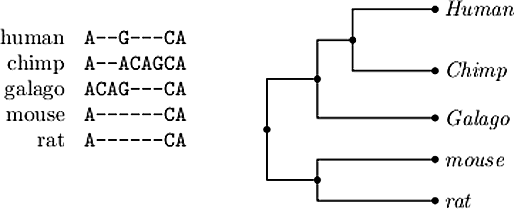
An example input to the indel history problem: An alignment of homologous extended sequences on the left, and the evolutionary tree for the species in the alignment on the right.

Table 1.

Comparison of Numbers and Frequencies of Events between Coding and Non-Coding Regions

	Total no. of sites	Total no. of bases	Total no. of events	Sum of event lengths	Indels/substitution ratio
Coding regions (from ENCODE)	156,607	931,938	661	2,343	0.01
Non-coding regions (CFTR)	209,381	1,438,546	2,851	8,160	0.11

The numbers for the coding regions were taken from a data set from ENCODE for the species human, chimp, galago, rat, mouse, and dog. The total number of events includes, in addition to insertions and deletions, also root events, which are events that cannot be determined uniquely as either insertions or deletions. The numbers for the non-coding regions were taken from non-coding regions around the CFTR gene for various primates.

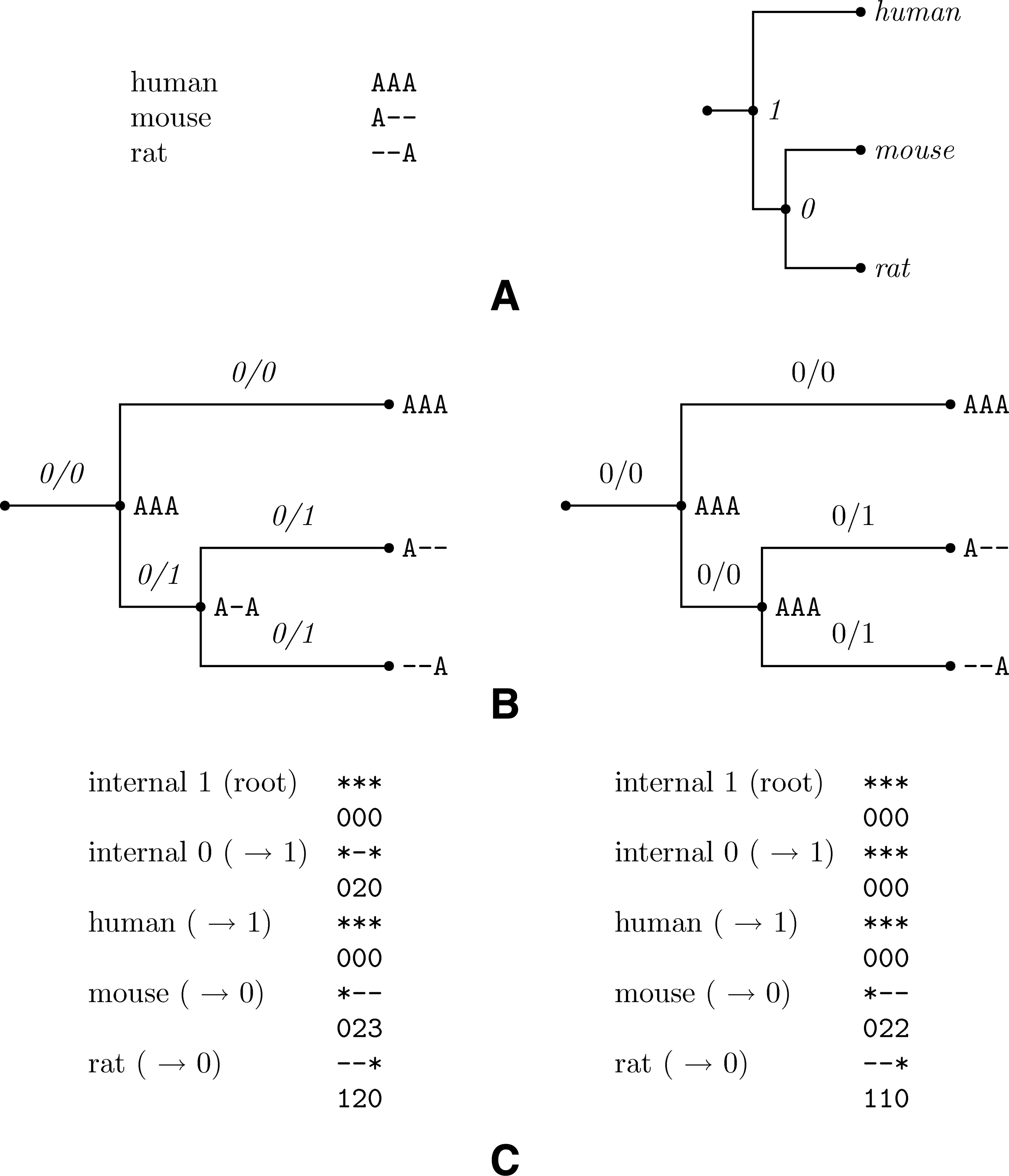
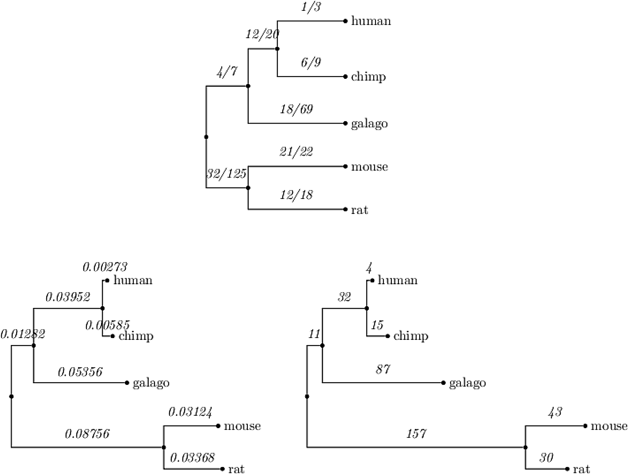
Note that we are not interested in the assignment of nucleotides to ungapped positions in the history; rather we simply care about the gaps. For this reason, we indicate ungapped positions by “*.” Figure 3 describes a possible history to the input of Figure 2.

FIG. 3.

history describing the input alignment of Figure 2 with respect to the given tree. As can be seen, the symbols at internal nodes distinguish only between a missing and existing base. The numbers along the branches indicate the number of insertions and deletions along each branch summed over the whole length of the alignment (in the form ins/dels). According to that history there was an insertion of AGC at sites 5–7 along the branch leading to the chimp and a deletion at sites 2,3 along the branch to the human-chimp ancestor.

For a given history, an insertion at some node is a succession of ungapped sites for which the same sites in the parent sequence are gaps. An example of an insertion is shown in Figure 3 in the sequence of the chimp where the inserted sequence is CAG at sites 5–7. Similarly, a deletion is a succession of gaps for which the parent sequence contains no gaps. An example of a deletion is shown in the ancestral sequence of the chimp and human, at sites 2–3. There is always ambiguity at the root of the tree as to whether an indel is an insertion or deletion, so such events are denoted by gaps. Every insertion, deletion or a gap constitutes an event. The score of a history is the number of events it induces on the input. A different view of our task is demonstrated by Figure 4. Indels create “holes” in the given alignment. Our task is to cover all the holes by associating events to the tree branches. Every event on an edge is associated with starting and ending column that indicate what hole it covers.

FIG. 4.

Another view of the input to the problem. (Top) A tree and an alignment with “holes” correspond to indels. (Bottom) Holes are covered by assigning events to the tree branches. The task is to cover all holes in the alignment.

We developed software, which takes as input an alignment and a phylogeny and produces an optimal history for that input. The output is in the form of an alignment including the inferred ancestral sequences. It is convenient to display summaries of the output, as in Figure 3. Figure 5 shows a toy example of an output of our software for finding a maximal history for a given input. The upper part of the figure shows a forty site alignment of human cow and dog and the corresponding phylogeny. The lower part shows the output produced by the software. In this example, there are five events and therefore the largest event number is five. The numbers under every site indicate the event associated with the site. As was explained above, a star represents an existence of a nucleotide and a “-” the opposite. However, in places where there was an insertion, the inferred base is plotted in uppercase letters, and in case of a deletion, it is plotted in lowercase.

FIG. 5.

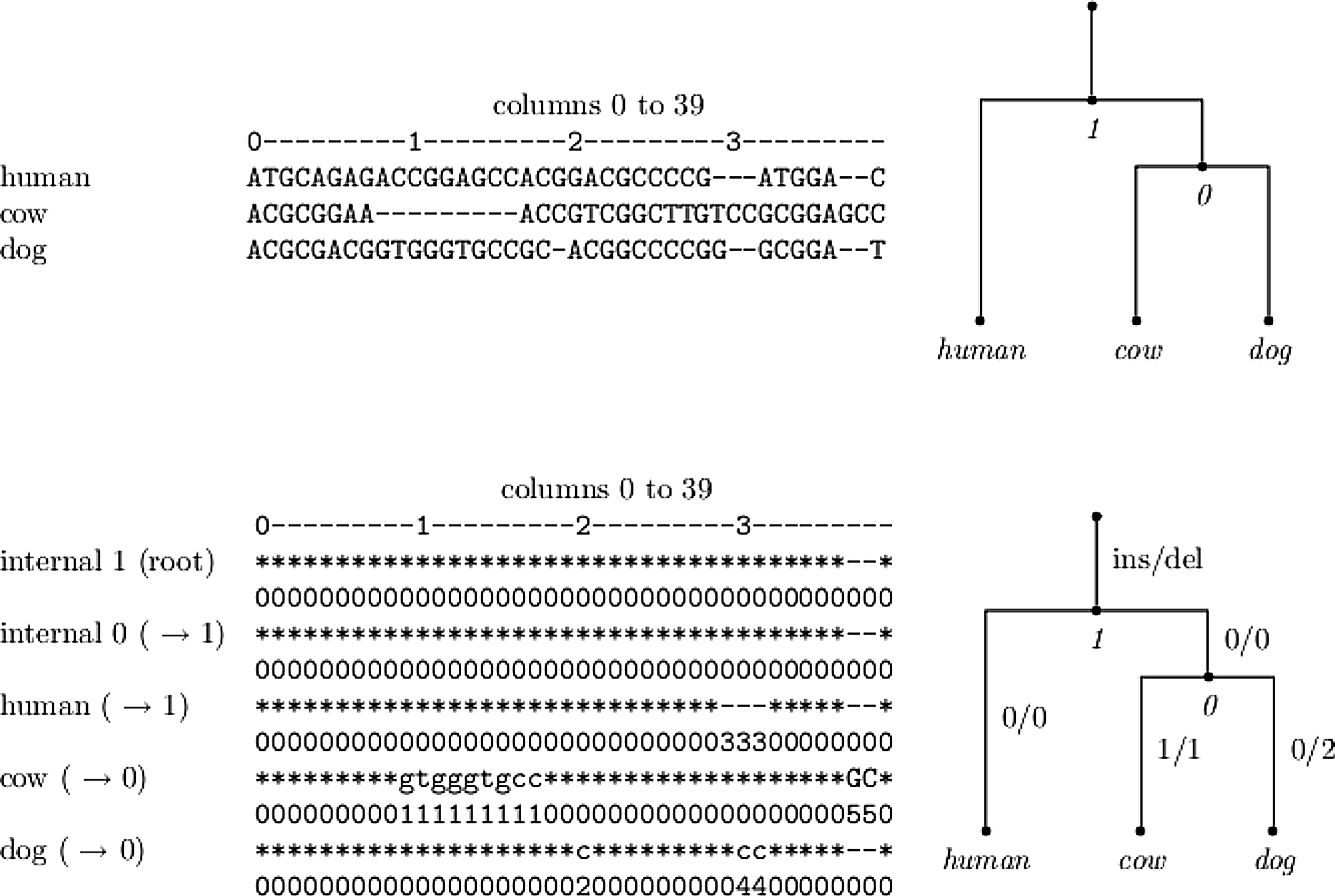
A toy example of the software output. On top, a 40-sites-long alignment of human, cow, and dog is displayed (left) and the corresponding phylogeny (right). At the bottom, the software output corresponding to the given input is displayed. In addition to the extant species, ancestral species are also displayed with the ancestral node besides every node name. The inferred optimal history is displayed in the centre. Stars (*) stand for an existing bases and dashes (-) for none. At positions (species and site) where an insertion was inferred (e.g., site 37 for cow) the inferred bases are displayed in uppercase and where a deletion was inferred (e.g., site 30 for dog), in lowercase. Every indel event is associated with a unique number arbitrarily (e.g., the deletion at the dog at sites 30–31 is assigned the number 4) where no-event positions (inherited from the root) are assigned number 0. Events from the root (e.g., site 29 at the human) are not interpreted as neither insertion nor deletion. At the bottom right, a summary of the events along the phylogeny branches is displayed in the form ins/del.

2.2. Previous work

Our aim here is to show how our findings compare to previous findings obtained on related data, first to show relevance of our approach, but also to enhance these results. We started with the deletion/insertion proportion compared in previous studies. Previous studies have already indicated the excess of deletions in comparison to insertions in both coding (Taylor et al., 2004) and non-coding regions (Thomas et al., 2003). We enforce these results but also reveal differences between the two types of regions. We start with coding regions. We applied our software to alignments of coding regions from ENCODE (see Methods) and obtained the number of events along all branches not emanating from the root. Since Taylor et al. (2004) considered only codon insertion and deletion events (i.e., indels of length divisible by 3), we filtered out all events of other lengths. The distribution of events obtained along the tree branches is shown in Figure 6 (top tree). The first value we examined is the ratio between insertions and deletions along each branch of the tree. The del/ins ratio at the mouse lineage is 1.05 (versus 1.1 obtained by Taylor et al. [2004]) and 1.5 at the rat (versus 1.7 obtained by Taylor et al. [2004]). The second value we measured is the frequency of events along a sequence. This measure should not be confused with the rate of events along a branch in the tree. The latter indeed measures the number of events with respect to the edge length (and therefore is proportional to evolutionary distance (Felsenstein, 2003), while the frequency of events ignores this factor. In our data, there were 108,000 codons for the rat and mouse sequences (twice the alignment length, 156,000 for both rat and mouse divided by 3) and a total of 73 events (sum of events for rat and mouse), yielding a frequency of one event per 1,479 codons (versus 1,736 obtained by Taylor et al. [2004]). The agreement is striking considering that our trees contain more than twice the number of species and four-fold more branches (eight vs. two, not counting branches emanating from the root), and events could have been attributed to other branches of the tree. While in Taylor et al. (2004), a gap in the mouse and human is automatically inferred as an insertion in the rat, in our method, based on the whole set of sequences, this scenario can be interpreted as a multi event site (see exact definition in the sequel) in which both mouse and human exhibit two different deletion events at that site.

FIG. 6.

Indel and point mutation statistics along the tree branches at coding regions. (Top) The tree on the upper part of the figure illustrates the distribution of indel events along the tree branches (in the form ins/del). Since the data corresponds to coding regions, events of length not divisible by 3 were eliminated. (Bottom left) Branch lengths correspond to the point substitution rate inferred according to the HKY model for the data. (Bottom right) Branch lengths correspond to the total number of indel events along the branches. The figure demonstrates the close link between the two processes. In order to obtain the ratio between point mutation rate and indel rate, we normalize the number of indel events by the alignment length 156,000 bases. The ratio found is 0.01 (Fig. 9).

Coding regions were also studied by Clark et al. (2007) on the human genome on the same data set we used the ENCODE. Indels were inferred by the shutgun re-sequencing reads and compared to point mutations. Although there was no distinction between insertions and deletions, the data relevant to our study is the distribution of indels in general along the genome. Clark et al. (2007) found that there are approximately 15 indel events per 100 kilo bp. This number is significantly smaller than our findings (Table 1). However, a closer look reveals that since our study included two rodent species and a galago that exhibit rates about 10 fold faster than human, a similar result is obtained. This also holds for average number of inserted bases that were found to be 43 per 100 kilo bp.

Our next comparison was to Cooper et al. (2004), who studied indel events among mouse, rat and human, and found a constant ratio between them to substitutions events. In Cooper et al. (2004), the rate of indel events is measured as the number of events per site, and substitution events are the rate of point substitutions per site (expressed as the length of the tree branch). This ratio, calculated only in the two pendant mouse and rat branches and along the whole genome, was found to be 0.05. Since our non-coding data was comprised of different, but closer species, we cannot make an exact comparison. Our non-coding data (on which we compared indels to branch lengths) is of two alignments of primate sequences in which ratios of 0.11 and 0.07 were found. Cooper et al. (2004) eliminated regions heavily gapped in either rodent, leading to an artificial reduction in the ratio computed, so we believe the agreement is satisfactory.

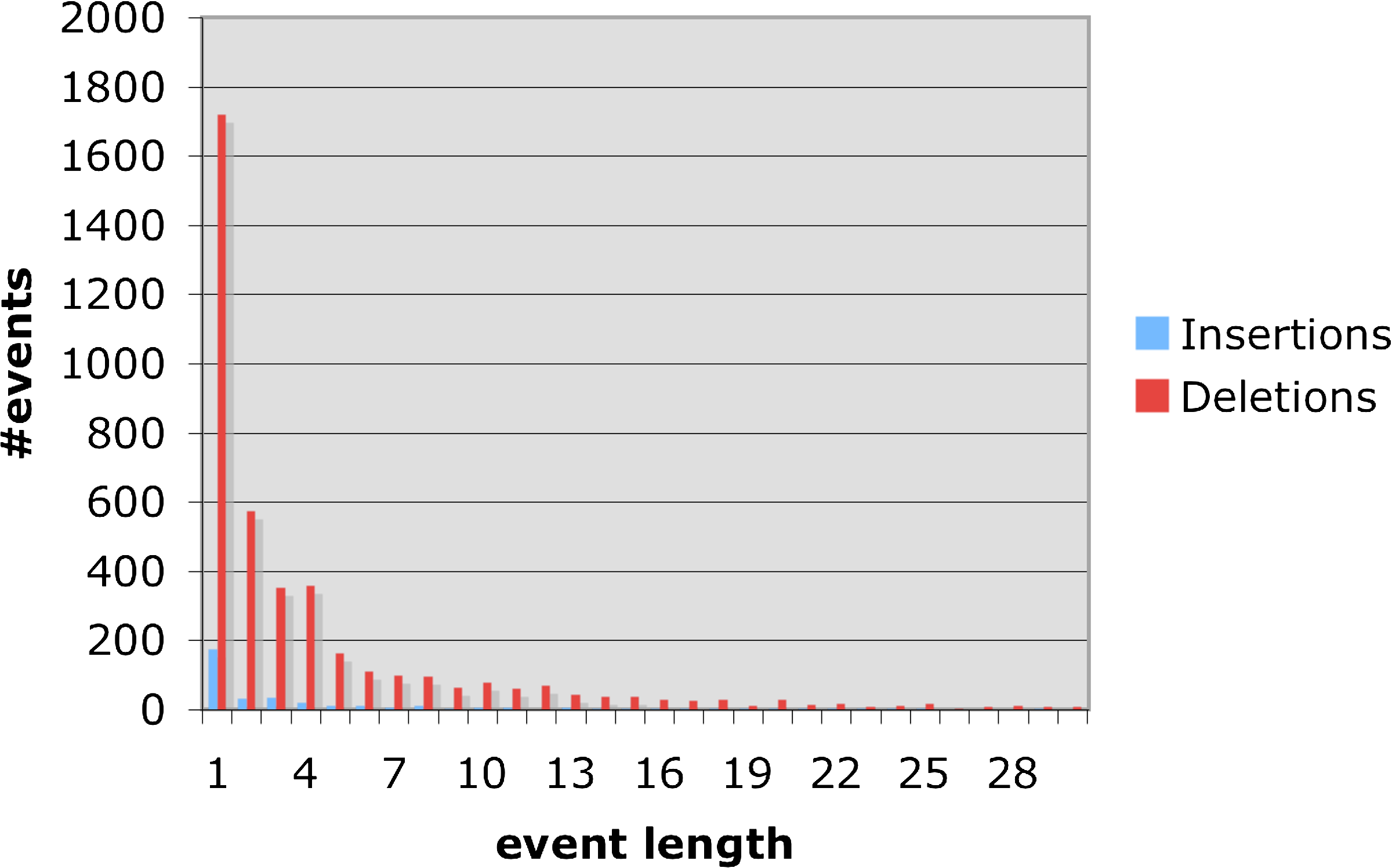
Cooper et al. (2004) present an exponentially decaying curve, describing the frequency of events as a function of their length. Figure 7 plots our findings with respect to this point in both coding and non-coding regions. The shape of the curve is very similar to the one in Cooper et al. (2004). We stress that our data summarizes events along all tree branches and hence endows it some more reliability.

FIG. 7.

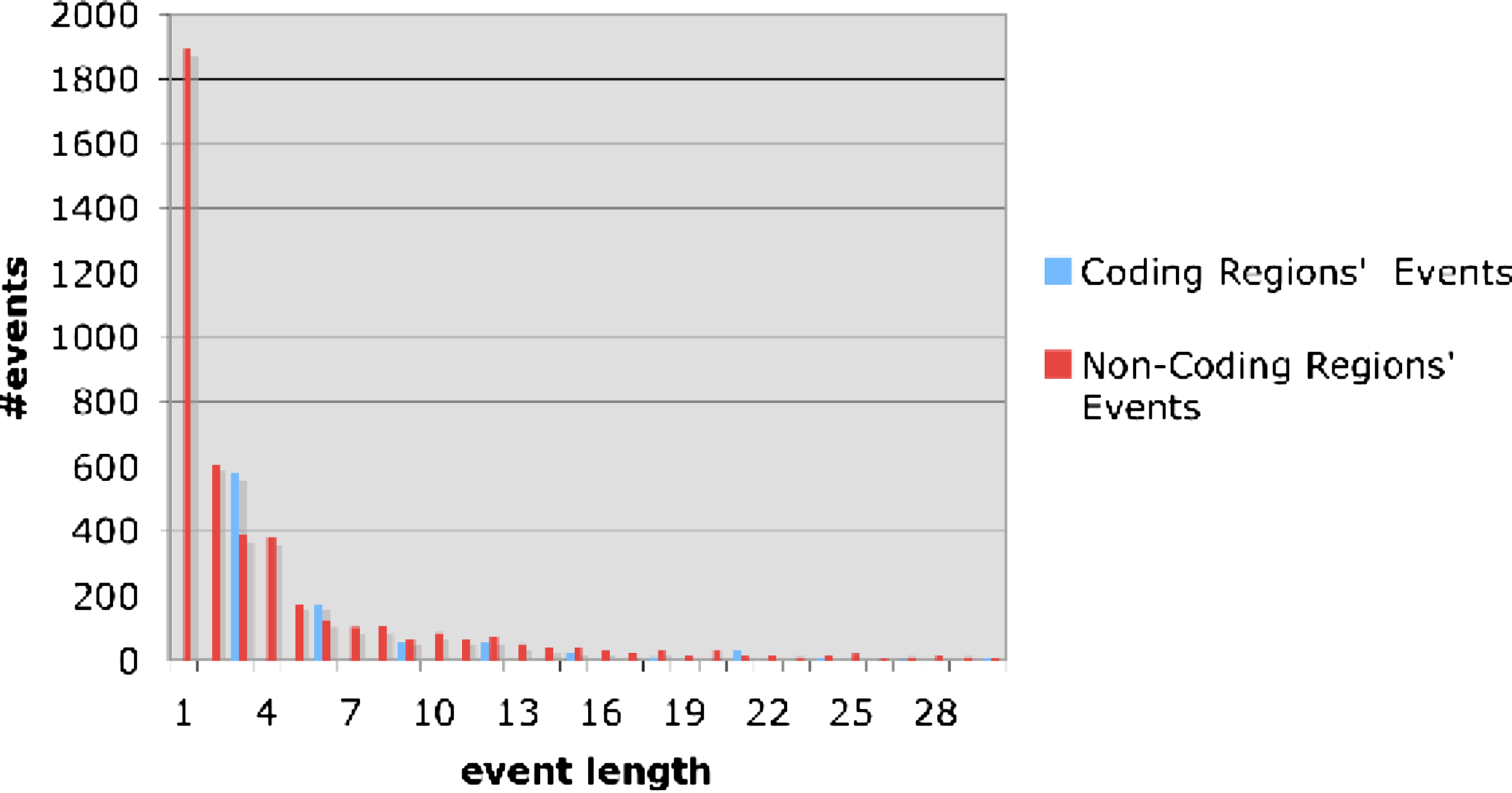
The distribution of the total number of events (insertions and deletions) as a function to event lengths. Red and blue blocks correspond to non-coding and coding regions respectively. Data obtained for all species and regions analyzed (not restricted to the species at Figs. 6 and 12). As can be noticed, frequency decreases exponentially with length.

2.3. Coding regions

As coding and non-coding regions differ both in the type of analysis and results, we report them separately. Figure 8 and Table 2 summarize our finding in coding regions. Both insertion and deletion frequencies decay exponentially with length. An exception to this exponential decay in the length is events of 7 codons (21 bases) that stand out in both insertions and deletions. We do not have an explanation for this. It can also be seen that deletions are slightly longer on average than insertions. We also wanted to measure if, and how, the rate of indels changes along the branches of the tree. We normalized the number of events on each tree edge, by the length of the edge. This measurement enables us to estimate the correlation between the length of an edge (the expected number of substitutions on the edge) and the number of indel events accumulated on it. Another question we examined is whether the indel process is homogeneous over time, or changes along different lineages of the tree. The ENCODE data contains many genes and different sets of species. In order to obtain enough information we concatenated multiple genes over a common set of species. Figure 6 at the top shows the number of indels along each edge of the tree. We used the same data in order to obtain the edge lengths corresponding to the tree, by ML estimate according to the HKY (Hasegawa et al., 1985) model. As the dog served as an outgroup to the rest of the species it was excluded from the figure. The tree on the bottom left of the figure shows the edge lengths inferred for the tree (measured by the expected number of substitutions along an edge). The edge lengths of the tree at the right bottom of the figure correspond to the number of indel (insertions plus deletions) events along the edges. The correlation between the edge length and the number of events is notable. Specifically, for every edge e, we computed the ratio ide/le where ide is the expected number of indel events per site along e and le is the length of e (the expected number of substitutions per site along it). We performed a linear regression between the ide and le values along the different edges. We found a ratio of 0.01 between ide and le with p ¡ 0.001 (Fig. 9). These results confirm the constant ratio found by Cooper et al. (2004), however, only at the two rodents branches whereas here we report this also for internal edges.

FIG. 8.

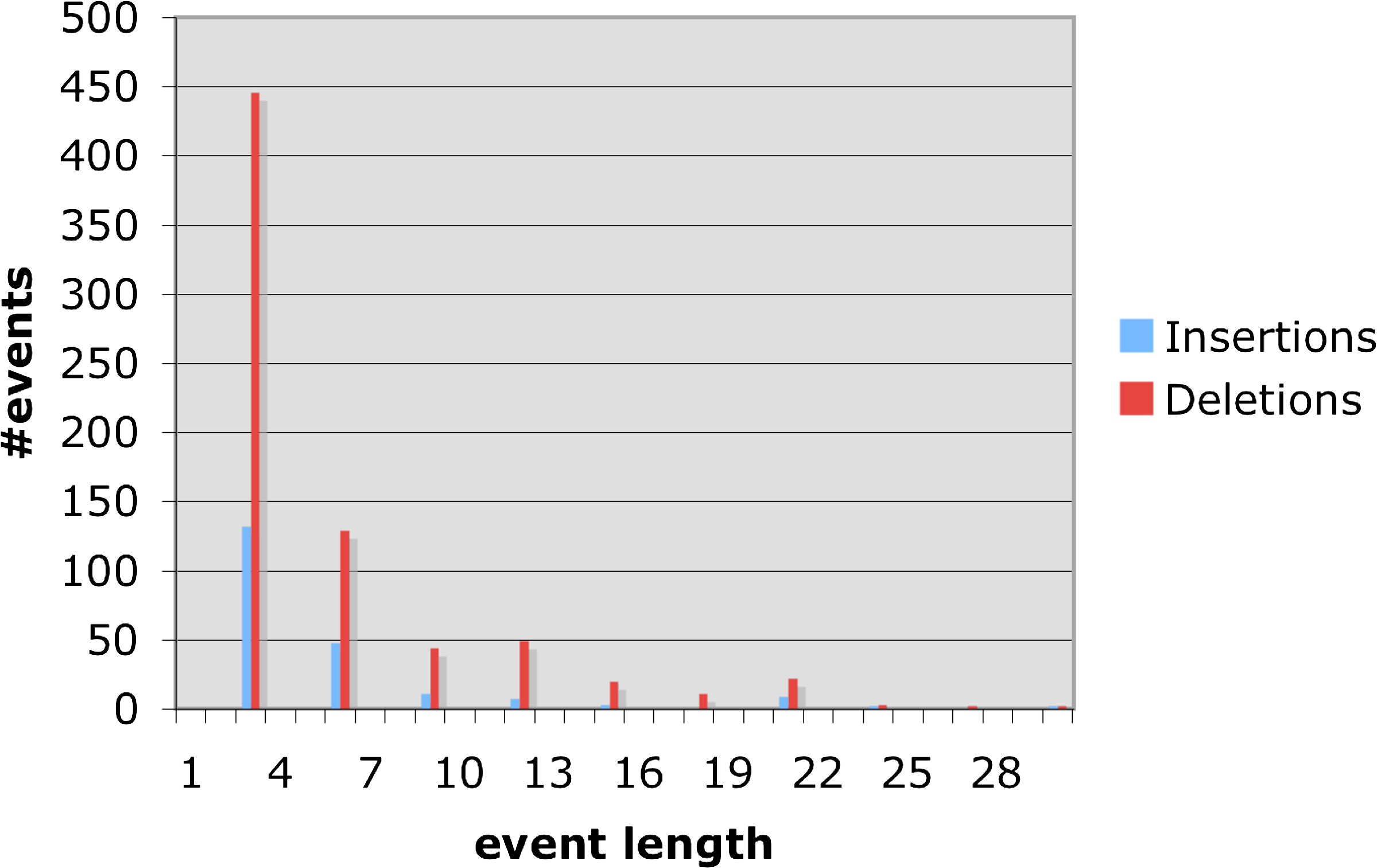
Frequencies of insertions/deletions in coding regions. Only events of length 0 mod 3 are reported.

FIG. 9.

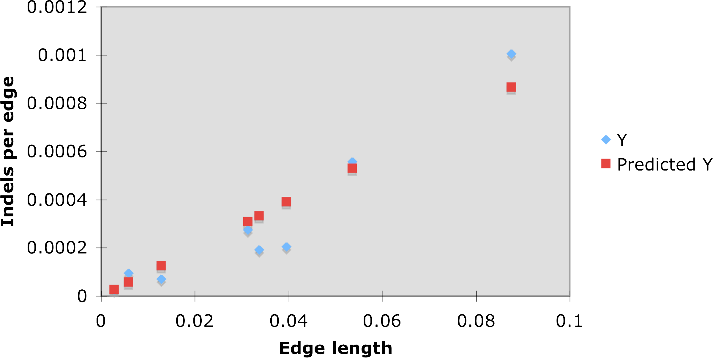
The linear regression analysis for the indel/mutation ratio at coding regions. The red line is the inferred ratio with slope 0.01 and p-value 0.0003 (confidence level 95%).

Table 2.

Events at Coding Regions (Only 0 mod 3)

Coding regions statistics
	Coding events distribution		Coding insertions distribution		Coding deletions distribution
Event length	No. of events	Total length per event	No. of events	Total length per event	No. of events	Total length per event
3	578	1734	132	396	446	1338
6	177	1062	48	288	129	774
9	55	495	11	99	44	396
12	56	672	7	84	49	588
15	23	345	3	45	20	300
18	11	198	0	0	11	198
21	31	651	9	189	22	462
24	5	120	2	48	3	72
27	2	54	0	0	2	54
30	4	120	2	60	2	60
Total	942	5451	214	1209	728	4242
Average event length		5.786		5.649		5.826

Except for events of 7 codons, the number of events decays exponentially with the length of the event. The average length of an event is 5.78 where average insertion is 5.65 bases and deletion 5.82 bases. The insertions/deletions ratio is 3.4.

In Saitou and Ueda (1994), it was postulated that the indel process obeys a molecular clock. This means that if we measure the length of the path along the tree, from any internal node to any of its descendants, this length will be the same. It is well known (Wu and Li, 1985) that with respect to point substitutions, this hypothesis does not apply to the set of species we investigated here. There was an acceleration in the rate of mutations in the rodents lineage after the speciation event from the primates. This causes a substitution rate twice as large in the rodents, than in the primates. The approximately constant ratio between ide to le refute the hypothesis of Saitu and Ueda (1994). In particular, it can easily be seen that the number of events on the path from the root to the mouse is exactly 200 while to the human it is only 47.

At the amino acid level, we examined whether there was a preference for certain kinds of insertions or deletions. The composition of amino acids in insertion and deletion events is depicted in Table 3. We inferred amino acid insertion/deletion in both extant species (i.e. in the aligned sequences) and the ancestral nodes. An event is determined to be an insertion/deletion by the optimal history (see Methods). The second and the third columns in the table display the actual number of times amino acids deleted/inserted respectively. The fourth and fifth columns display its relative weight in the insertion/deletion (respectively) processes. The sixth column is its frequency in the sequences examined (i.e. the background frequency). The last two columns normalize columns four and five by the background frequency. This allowed us to check whether an amino acid is over or under represented in either process. Figure 10 depicts the last two columns of Table 3 graphically. The green line at level of 1 signifies neutrality. It is notable that some amino acids maintain the same ratio in both processes (e.g., Arginine, Serine, Threonine), although this deviates from a neutral rate of relative value of one (e.g., Arginine, Serine, Phenylalanine). Another characteristic is that most of the amino acids are either overrepresented or underrepresented in both insertions and deletions. Since both insertions and deletions are almost uniformly distributed on both sides of the neutrality line, the probability of observing sixteen out of the twenty amino acids over or under represented by chance in both processes is 0.0046. Exceptions include Cysteine, Valine, and Glutamic Acid that are overrepresented in one process but underrepresented in the other. Table 4 depicts the distribution of the bases in the indel process. It can be seen that G-C are overrepresented (above their relative frequency in the population) in both insertions and deletions, while T is underrepresented in both processes and A is underrepresented in deletions and almost neutral in insertions.

FIG. 10.

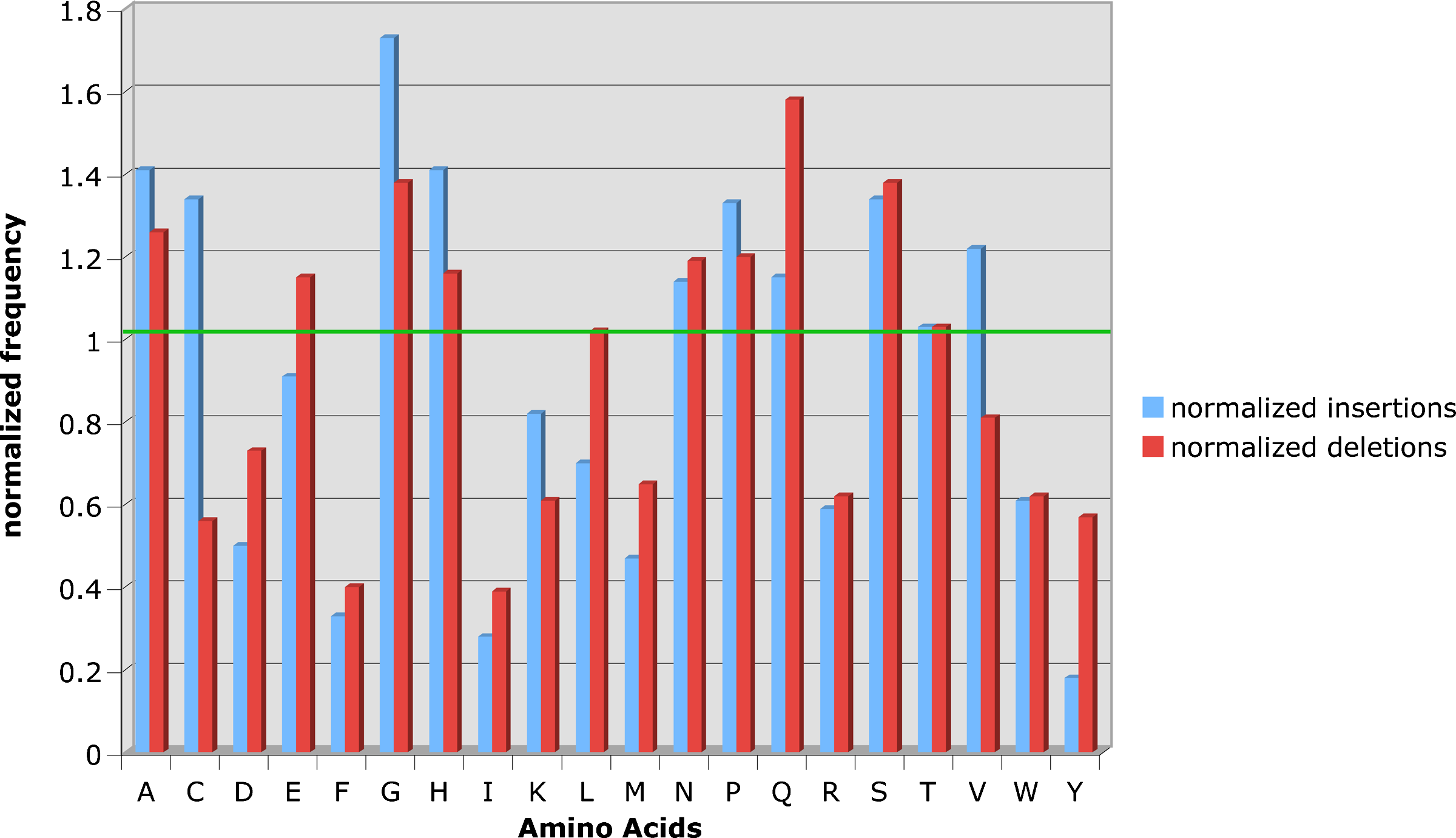
Normalized representation of amino acids in insertions and deletions. The frequency of an amino acid in either process was normalized in its background frequency. The green line represents neutrality, meaning an amino acid is inserted/deleted the same as it appears in the population. It can be seen that most of the amino acids are either over or underrepresented in both insertions and deletions.

Table 3.

Indel Statistics for Amino Acids

Indel statistics for amino acids
AA	No. of insertions	No. of deletions	Percent in insertions	Percent in deletions	Percent in population	Relative insertion	Relative deletion
A	45	133	10.56	9.38	7.41	1.41	1.26
C	10	14	2.34	0.98	1.73	1.34	0.56
D	10	48	2.34	3.38	4.59	0.5	0.73
E	28	117	6.57	8.25	7.16	0.91	1.15
F	5	20	1.17	1.41	3.52	0.33	0.4
G	49	129	11.50	9.1	6.56	1.73	1.38
H	15	41	3.52	2.89	2.47	1.41	1.16
I	5	23	1.17	1.62	4.05	0.28	0.39
K	19	47	4.46	3.31	5.37	0.82	0.61
L	30	143	7.04	10.09	9.89	0.7	1.02
M	5	23	1.17	1.62	2.47	0.47	0.65
N	16	55	3.75	3.88	3.24	1.14	1.19
P	39	116	9.15	8.18	6.78	1.33	1.2
Q	24	108	5.63	7.62	4.82	1.15	1.58
R	15	52	3.52	3.66	5.91	0.59	0.62
S	49	166	11.50	11.71	8.48	1.34	1.38
T	24	79	5.63	5.57	5.4	1.03	1.03
V	33	73	7.74	5.15	6.28	1.22	0.81
W	3	10	0.70	0.7	1.13	0.61	0.62
Y	2	20	0.46	1.41	2.46	0.18	0.57

The second and the third columns in the table display the actual number of times amino acids deleted/inserted respectively. The fourth and fifth columns display its relative weight in the insertion/deletion (respectively) process. The sixth column is its frequency in the sequences examined (i.e. the background frequency). The last two columns normalize columns four and five by the background frequency.

Table 4.

Distribution of Bases in Insertions and Deletion Events in Coding Regions

Base Distribution in Indel Processes
	% in population	% in insertions insertions	% insertions relative to percentage in population	% in deletions	% deletions relative to percentage in population
A	25.5	23.9	0.93	26.1	1.02
T	21.4	19.9	0.93	18.3	0.85
C	26.3	27.9	1.06	27.4	1.04
G	26.6	28.2	1.06	28	1.05

Table 5 and Figure 11 depict the statistics obtained for the non-coding regions we analyzed. There were 4465 events with a total length of 19534 bases, yielding an average of 4.37 bases per event. Events of a single base comprised 42.4 percent of the total number of events and of length two, 13.5 percent. Of the total number of events, there were 362 insertion events with a total length of 1697, yielding an average insertion size of 4.68 bases. There were 4103 deletion events with a total length of 17837, yielding an average deletion length of 4.34 bases.

FIG. 11.

Frequencies of insertions/deletions in non-coding regions.

Table 5.

Event Statistics at Non-Coding Regions

Non-coding regions statistics
	Coding events distribution		Coding insertions distribution		Coding deletions distribution
Event length	No. of events	Total length per event	No. of events	Total length per event	No. of events	Total length per event
1	1895	1895	174	174	1721	1721
2	606	1212	33	66	573	1146
3	388	1164	35	105	353	1059
4	379	1516	20	80	359	1436
5	175	875	12	60	163	815
6	123	738	11	66	112	672
7–12	500	4619	34	303	466	4316
13–18	224	3403	20	302	204	3101
19–30	175	4112	23	541	152	3571
Total	4465	19534	362	1697	4103	17837
Average event length		4.37		4.68		4.34

Table 6 depicts statistics of the composition of the bases in the indel events in non-coding regions. We used the same method here for the inference of the content of the indel events as for coding regions, except for the fact that we did not eliminate events with lengths not divisible by 3. We found that the GC content in indels was lower than the genome frequency. In insertion events, C is substantially underrepresented (0.81 of its genome frequency), while T is similarly overrepresented (1.13). In deletion events, both A and T are similarly overrepresented (around 1.05 of their background frequency) while C and G are similarly underrepresented (0.92). C and T exhibit the largest variation between insertions and deletions.

Table 6.

Distribution of Bases in Insertions and Deletion Events in Non-Coding Regions

Base distribution in indel processes non-coding regions
	% in population	% in insertions insertions	% insertions relative to percentage in population	% in deletions	% deletions relative to percentage in population
A	28.3	30.6	1.08	30.3	1.06
T	29.5	33.3	1.13	30.8	1.04
C	20.8	17.0	0.81	19.1	0.92
G	21.2	18.9	0.89	19.6	0.92

Similarly to coding regions, we wanted to measure the correlation between rate of indel events to the rate of point substitutions along the tree branches. Figure 12 depicts our findings in the CFTR region (ENCODE region number 1). The upper part of the figure depicts the distribution along the tree edges. The edge lengths of the tree in the lower left part correspond to the point substitution probabilities and at the lower right side, to the total number of indel events. As can be evidenced, both trees are more “clock like.” We were interested in the ratio ide/le for every edge e. Again by linear regression we obtained a value 0.11 with p-value 4.3E-7 (Fig. 13).

FIG. 12.

Indel and point mutation statistics for non-coding regions, taken from around the CFTR gene. The interpretation of the figure is identical to that of Figure 6 except that all events were counted. A significant bigger indel/mutation rate ratio of 0.11 is obtained (Fig. 13). Indels on branches were normalized by alignment length of 209,000 bases.

FIG. 13.

The linear regression analysis for the indel/mutation ratio. The red line is the inferred ratio with slope 0.01 and p-value 0.0003 (confidence level 95%).

2.4. Multi-event sites

From probabilistic perspective, several events occurring at the same site are not very likely. We denote these as multi-event sites (MES); that is, sites where indel events have occurred on more than one branch of the tree. Indel events (as opposed to the sites) at MES sites are called parallel events. For a deletion, this definition is straightforward: A deletion event at a branch is parallel (to another event) if it deletes a nucleotide that was either inserted at some ancestral branch or has a homolog that was deleted at a non-ancestral branch. However, as for insertions, this definition is a bit more complicated. An insertion at a branch is considered parallel to another insertion event if it occurs between the sites flanking the other event (note that if the other event is not ancestral to the first, the two sites flank both events). An insertion at a branch is considered parallel to ancestral deletion if it occurs between the sites flanking the deletion, and parallel to a non-ancestral deletion if the sites deleted flanking the insertion.

MES can cause confounding input to our algorithm that might yield a wrong history. Consider the case of insertion inside an insertion as illustrated in Figure 14. The root node has two nucleotides “15,” an insertion of “24” results in “1245” at a descendant, and the second subsequent insertion of “3” results in “12345” at a descendant of the later. Note however that the problem of inferring optimal history is not constrained to specific sequences at ancestral nodes, as is described in the Method section, rather only to sequences at the leaves. Hence, translating the scenario above to a representative input yields the input at Figure 14A, where the sequences at the root and its direct descendant sit at leaf children of each such node. The real history appears at Figure 14B. It is important to note that this history yields a sequence of three events by the scoring algorithm, which is in contrast to the sequences that gave rise to that history. However, a closer look reveals that this input admits a different, more parsimonious history of two events as illustrated in Figure 14C. This example demonstrates that indeed the most parsimonious history is not necessarily the correct history, but the number of events produced is not larger than the number of original events.

FIG. 14.

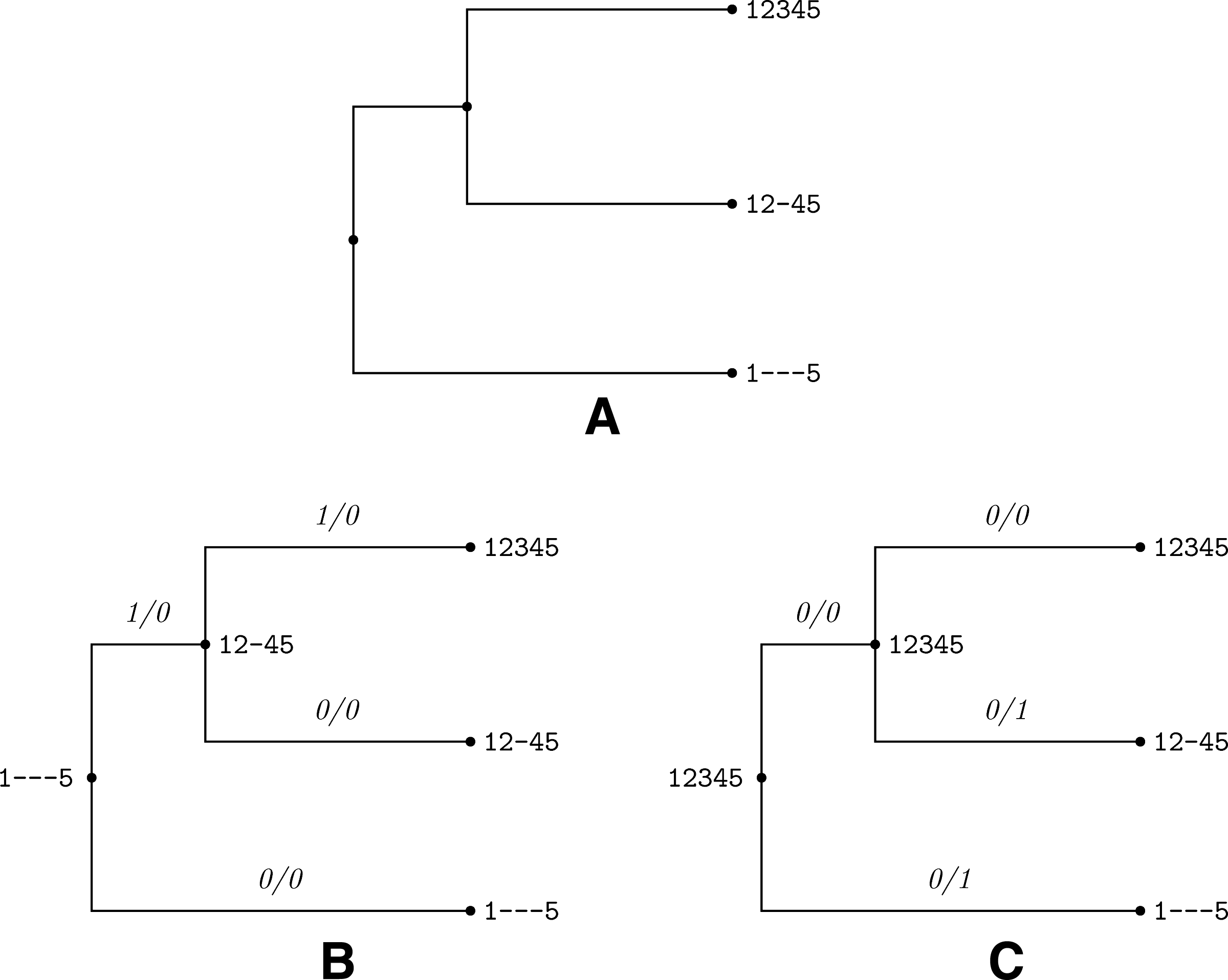
The most parsimonious history is not necessarily the true scenario. (A) shows the imprint of a sequence of two insertion events shown in (B). This scenario gives rise to three spurious events by our counting principle. However, a more parsimonious history for that input can be found as in (C), with the same number of events as in the original scenario.

Since alignment programs never place parallel insertions at the same sites (since this causes non-homologous bases to overlap), our calculations underestimate the number of parallel events. However, as insertions are less frequent than deletions and in particular insertions occurring in parallel to other events, we believe our estimates are fairly accurate. Our findings show that in both datasets, the frequency of parallel events was above two fold the expected value. Specifically, for coding regions, the number of sites containing a single event was 9,553, yielding an expected value of 0.0295 (the total number of sites in all datasets analyzed was 323,673) and a probability of 0.000871 of finding a parallel event at a site. The actual number of sites containing parallel events was 1093, yielding a frequency of 0.00337 parallel events per site, 3.876 times its expected value. For non-coding regions, we found 30,616 sites containing an event, yielding a frequency of 0.0714 sites containing events, and a probability of 0.0051 for a parallel event at a site. The actual frequency of parallel events was 0.0111, which is 2.178 times the expected value. These findings are consistent with the findings of Taylor et al. (2004) about the effect of slippage at indel events. Taylor et al. (2004) found that the frequency of indel events is about 50% higher than expected in proximity to small regions where the same amino acid is duplicated. As we have shown, such indel “hot spots” are also evident in non-coding sites. It is interesting to note that Lytynoja and Goldman (2005) argue against evidence for indel hot spots, suggesting that they are the result of alignment artifacts. While we do not argue with Lytynoja and Goldman (2005) findings, we believe that our results confirm the existence of indel hotspots.

3. Conclusions

In this work, we have used the algorithm developed in our previous work for further studying of most parsimonious indel history. We demonstrated by simulation that this approach is sound when the analyzed data pertains to evolutionarily closely related species. Subsequently, we analyzed alignments taken from both coding and non-coding regions and discussed implications stemming from multi-event sites. The points below summarize several issues arising from this research.

3.1. Differences between coding and non-coding regions

Table 1 depicts major differences we found between indels inside coding and non-coding regions.

3.1.1. Insertion/deletion ratio

The difference between the rates of insertions and deletions has been mentioned many times in the past; however, it was believed to be constant in different regions (Blanchette et al., 2004). Our first remarkable observation is that the ratio between the rates of insertions and deletions changes substantially from 2.47 del/ins in coding regions to 11.23 del/ins in non-coding regions. We note that we did not find significant shifts in the behavior of the processes along the tree branches in both regions. We comment that indel variation was also observed by Chen et al. (2009); however, our analysis extends theirs also to the tree branches.

3.1.2. Indels average length

The average length of events differs between coding and non-coding regions. In general, the average length of an event is larger in coding regions and is 5.78 versus 4.37. This can be attributed directly to the prevalence of single base events in non-coding regions where these events are deleterious in coding regions. Another interesting difference is the ratio between the lengths of an average insertion to average deletion in both regions. While in coding regions the average insertion length is 5.649 and 5.826 for deletion, in non-coding regions, insertion length is 4.68 versus 4.34 for deletion.

3.1.3. Ratio between indel events rate to mutation rate

The ratio between indel events rate to mutation rate, ide/le also changes substantially between the two region types. Indeed this ratio at non-coding regions is also changing among the different data sets we considered (CFTR, LDLR, CETP, APOA1, etc.). However, the variability was relatively moderate centered around the value of 0.13. This is to be compared to a ratio of 0.013 in coding regions (0.01 disregarding non 0 mod 3 events). Some explanation to this is the fact that while coding regions are under very high selective pressure against indels in general and non 0 mod 3 specifically, they allow for a high rate of synonymous point substitutions that may cause a shift down in the value of ide/le at these regions.

3.2. Estimating the size of ancestral genomes

Since we know the ratio between point mutation rate and indel rate, and have noted that this ratio is unchanged with time, we can compute how many indel events are accumulated in a certain amount of time. Knowing the ratio between the rates of insertions and deletions and the average lengths of both events, enables us to calculate by how much the genome is contracting due to indels. A similar question was studied by Grover et al. (2008) focusing on two cotton species by considering also large scale mutational events. The question was also addressed from a different point of view by Petrov et al. (2000) who tried to explain differences in genome sizes of the Drosophila and Hawaiian crickets (Laupala) by the differences in the indel profile (ide/le, differences between insertion and deletion rates, differences in average sizes). We pursue a similar approach with the aim of estimating DNA loss due to indels.

Since coding regions comprise a small amount of the genome, and in addition both the rate of indels ide/le is low and the difference between insertion and deletion rate is small, it suffices to consider only non-coding regions. We rely on our finding that there has been no significant shift in the effects of indel processes with time, and take the ide/le value obtained for the CFTR region: 0.11. In non-coding regions we have a ratio of approximately 11 between deletions to insertions, yielding an expected decrease of 3.58 bases per indel event [(11*4.34 4.68)/12]. This boils down to a decrease of 0.394 bases (0.11*3.58) per one expected substitution. This implies that for an evolutionary distances of 1 expected substitution per site, only 0.606 of the bases that existed in the ancestral sequence even survived. ENCODE region 1 contains data from various species for the CFTR extended region. The length of the path from the human to the human- zebrafish ancestor in the tree is 0.891. By the above analysis we find that 0.35 of the human-zebrafish ancestral sequence disappeared due to micro-indels events. Of course, the extant genomes have also been subjected to transposable element duplication, and other large scale duplications which have presumably drastically altered the size and content of the genomes.

4. Methods

4.1. The Data

As was explained above, our approach requires working with evolutionarily close sequences. Hence alignments for coding regions of a set of vertebrates were obtained from the ENCODE project (ENCODE Project Consortium, 2004, 2007) (http://genome.ucsc.edu/ENCODE/). These alignments were re-aligned to ensure consistency of codon alignments. For non-coding regions, a large set of primate sequences was required. ENCODE region 1 contains aligned sequences of ten primates. Additionally, sequences flanking various genes such as LDLR, CETP, APOA1, etc., in primates were obtained from the Programs for Genomic Applications (PGA) database at Lawrence Berkeley National Laboratories (http://pga.jgi-psf.org/seq/). These were aligned with MAVID (Bray and Pachter, 2004) (http://bio.math.berkeley.edu/mavid/download/). We also made use of two recent primate intron data sets from the PAX9 gene and the MSX1 gene, analyzed by Perry et al. (2006). These alignments contain 15 and 14 species, respectively.

4.2. Computing the optimal history

We now describe our algorithm for computing the optimal history for a given alignment of length n (number of sites) for a set of m species, and a phylogeny for the species. As was mentioned above, a history is an assignment of extended sequences (sequences composed of stars for base presence, and dashes for absence) to the internal nodes of the phylogeny. The length of the history is defined to be the length of the alignment, or alternatively, the length of each extended sequence in the history. A position is defined as a specific site at a sequence (either from the alignment, or from the extended sequences of the history). The ancestor of a position p at sequence s, denoted a(p), is the position of the same site at the sequence ancestral to s (as defined by the phylogeny). The left of a position p at sequence s, denoted l(p), is the position at the same sequence but one site before.

We start by describing a simple algorithm to compute the score of a given history of length n. (Note that this is not an algorithm for finding an optimal history rather for evaluating a given history.) Given a history, the number of events in the history can be computed by proceeding along the history from left (site number 1) to right. At every site, for every position p, with ancestral a(p), we define the sign of the position p as follows: \documentclass{aastex}\usepackage{amsbsy}\usepackage{amsfonts}\usepackage{amssymb}\usepackage{bm}\usepackage{mathrsfs}\usepackage{pifont}\usepackage{stmaryrd}\usepackage{textcomp}\usepackage{portland,xspace}\usepackage{amsmath,amsxtra}\pagestyle{empty}\DeclareMathSizes{10}{9}{7}{6}\begin{document}\begin{align*} sign (p) = \begin{cases} \quad 0 &\ \hbox{if under the history both} \ {\it p}" \ {\rm and} \ {\it a(p)} \ \hbox{are, either gapped or both are non gapped}, \\ \quad 1 &\ \hbox{if under the history} \ {\it p}" \ \hbox{is non gapped but} \ {\it a(p)} \ \hbox{is gapped}, \\ \ - 1 &\ \hbox{if under the history} {\it a} \ ({\it p})" \ \hbox{is non gapped but} \ \it {p} \ \hbox{is gapped}.\end{cases} \end{align*}\end{document}

Note that sign is computed at every site and every node, except the root of the tree (because the root has no ancestral node). Given a history h, after computing the sign of a position p under h, it is possible to compute the event number at p, denoted event(p). The event number at every position at the roots extended sequence is defined to be 0. The event at every position at the first site (site 1) is determined by a top down fashion as follows: \documentclass{aastex}\usepackage{amsbsy}\usepackage{amsfonts}\usepackage{amssymb}\usepackage{bm}\usepackage{mathrsfs}\usepackage{pifont}\usepackage{stmaryrd}\usepackage{textcomp}\usepackage{portland,xspace}\usepackage{amsmath,amsxtra}\pagestyle{empty}\DeclareMathSizes{10}{9}{7}{6}\begin{document}\begin{align*} event (p) = \begin{cases}event (a(p)) & {\rm if} \ sign (p) = 0 \\ \hbox{new event number} & \hbox{otherwise}\end{cases} \end{align*}\end{document}

The process continues now from left to right and top to bottom. For a position p for which the event number of its ancestral position a(p) and the position to its left l(p) have already been determined, the event number is computed by: \documentclass{aastex}\usepackage{amsbsy}\usepackage{amsfonts}\usepackage{amssymb}\usepackage{bm}\usepackage{mathrsfs}\usepackage{pifont}\usepackage{stmaryrd}\usepackage{textcomp}\usepackage{portland,xspace}\usepackage{amsmath,amsxtra}\pagestyle{empty}\DeclareMathSizes{10}{9}{7}{6}\begin{document}\begin{align*} event (p) = \begin{cases}event (a (p)) &{\rm if} \ sign (p) = 0 \\ event (l (p)) &{\rm if} \ sign (p) \neq 0 \ {\rm but} \ sign (p) = sign (l (p)) \\ \hbox{new even number} &\hbox{otherwise}\end{cases} \end{align*}\end{document}

Upon completing the last site, the cost of the given history is the number of new events. As can be evidenced from the algorithm, this cost is computed by the cost of the site previous (or left) to the site currently checked, plus the cost of moving to the current site (that is, the number of new events incurred by that move). This defines a recurrence relation to compute the cost of a history. However, finding the optimal assignment (history) is a more complicated task even though it uses the same recurrence relation. For this end, we define the notion of a slice of a history. The slice of a history h at a site s, is the value (under h) of all the positions at s. For two slices at two adjacent sites, with history slices s and s, we define the cost of the two slices as follows: \documentclass{aastex}\usepackage{amsbsy}\usepackage{amsfonts}\usepackage{amssymb}\usepackage{bm}\usepackage{mathrsfs}\usepackage{pifont}\usepackage{stmaryrd}\usepackage{textcomp}\usepackage{portland,xspace}\usepackage{amsmath,amsxtra}\pagestyle{empty}\DeclareMathSizes{10}{9}{7}{6}\begin{document}\begin{align*} cost (s , s^{\prime}) = \sum_{v \in V (T) \setminus \{r \}} \mid sign (s^{\prime} , v) \mid \cdot \bar{\delta}_{sign (s , v) , sign (s^{\prime} , v)} , \end{align*}\end{document}

where \documentclass{aastex}\usepackage{amsbsy}\usepackage{amsfonts}\usepackage{amssymb}\usepackage{bm}\usepackage{mathrsfs}\usepackage{pifont}\usepackage{stmaryrd}\usepackage{textcomp}\usepackage{portland,xspace}\usepackage{amsmath,amsxtra}\pagestyle{empty}\DeclareMathSizes{10}{9}{7}{6}\begin{document}\begin{align*} \overline{\delta}_{x , y} = \begin{cases}0 &{\rm if} \ x = y \\ 1 &{\rm otherwise}\end{cases} \end{align*}\end{document}

It can be noted that cost(s, s) is the number of new events introduced by moving from slice s to s. Eventually, we define by opt(s, i) the cost of the optimum history up to site i under the constraint that the slice at character i is s. Then we can see that: \documentclass{aastex}\usepackage{amsbsy}\usepackage{amsfonts}\usepackage{amssymb}\usepackage{bm}\usepackage{mathrsfs}\usepackage{pifont}\usepackage{stmaryrd}\usepackage{textcomp}\usepackage{portland,xspace}\usepackage{amsmath,amsxtra}\pagestyle{empty}\DeclareMathSizes{10}{9}{7}{6}\begin{document}\begin{align*} opt (s , i) = \min_{s^{\prime}} [ opt (s^{\prime} , i - 1) + cost (s^{\prime} , s) ] . \end{align*}\end{document}

That is, opt(s, i) is obtained by finding the slice s that minimizes the number of events up to site i1 plus the number of events introduced by moving from s to s. Assume now that the length of the alignment is n and we define by opt the score of the optimal history. Then we find: \documentclass{aastex}\usepackage{amsbsy}\usepackage{amsfonts}\usepackage{amssymb}\usepackage{bm}\usepackage{mathrsfs}\usepackage{pifont}\usepackage{stmaryrd}\usepackage{textcomp}\usepackage{portland,xspace}\usepackage{amsmath,amsxtra}\pagestyle{empty}\DeclareMathSizes{10}{9}{7}{6}\begin{document}\begin{align*} opt = \min \limits_{s} opt (s , n) . \end{align*}\end{document}

After the last character has been processed, the most parsimonious history found is reconstructed by tracing backward the optimal solutions that constituted the final solution.

The uniqueness of the solution is a serious issue in this type of computation. A solution is unique if when tracing backward to reconstruct the optimal solution, at every site i for which the optimal solution inferred the slice s, there is a unique s′ satisfying opt(s, i) = opt(s, i − 1) + cost(s, s). Our algorithm keeps the first optimal value encountered. This might lead to a discrepancy between two optimal solutions as to the specific events along the tree edges (although, not as to the whole tree, by definition of the optimality). In practice, we computed two extreme optimal solutions and took the average. In brief, one approach is star-favoring while the other is dash-favoring. Except for branches emanating from the root the difference between the two solutions was not significant.

The running time of the algorithm on an input alignment of m species and n sites is O(n^2m − 2) since for every two adjacent sites we check for all possible history slices for these sites which amount to 2^2m − 2 (we considered only binary trees in which the number of internal nodes is m − 1). More details are available in Snir and Pachter (2006).

4.3. Simulation results

In order to test the viability of our approach, we designed a sequence simulator tailored specifically for our purposes. The simulator distinguishes between coding to non-coding regions and generates events according to the event frequencies we observed in both regions (see Results). The input to the simulator contains a phylogeny with branch lengths, an indication for coding or non-coding region and event length distribution tables for insertions and deletions. The simulator generates an indel history in a top-down manner as follows:

∘ The root of the tree is assigned a sequence of ungapped bases.

∘ For every node whose ancestor has been processed:

Let p_e be the event probability for the edge (obtained by the id_e/l_e ratio for the region simulated times the length of the edge entering the node).

At every ungapped base, with probability p_e open an event. Otherwise, copy the type of base at the ancestral node.

∘ Output the (aligned) sequences at the leaves.

Given the simulator output to an algorithm, we consider a reconstruction to be correct if for both insertions and deletions the number of events inferred for every length is the same as was generated by the simulator (note that this does not require a perfect reconstruction of the original history). We believe this is a more accurate measure than counting the percentage of positions at which the original value (star or dash) was reconstructed.

We tested our algorithm on with two trees of ten species. The first tree was chosen from the 27 vertebrates tree from ENCODE region 1 with accumulated edge length of 3.56. The second was derived from the 15 primates tree of Perry et al. (2006) with accumulated edge lengths of 0.49. We used the first tree to simulate events in coding regions and the second in non-coding regions. For each region, 30 alignments were generated. In the coding experiment 3211 events were simulated out of which 97% were reconstructed. In the non-coding regime, 1399 events were simulated, out of which 88% were reconstructed. Due to the stringent comparison metric, we believe this is a fairly good reconstruction ratio.

4.4. Scalability

The current phase of the ENCODE project was a pilot for a whole genome analysis. We therefore considered practical approaches for scaling our analyses. A first significant improvement is achieved by the following property: it can be shown that there exist optimal histories in which identical adjacent sites induce the same ancestral history. That means that by advancing along identical sites in the alignment, we do not acquire new events. Therefore, we can contract every two adjacent identical sites in the input alignment into one. The above operation yields an alignment in which every two adjacent columns (sites) are non identical. After the optimal history is found, the compact alignment is expanded to its original form. Moreover, since at every site in the compact alignment, at least one event is either starting or terminating, the length of this alignment is at most twice the number of events in the optimal history. This improvement was particularly useful in coding regions where it rendered about 100 fold shorter alignments (mostly due to very long segments without any gap).

The exponential factor in the running time can pose a serious drawback on the method and makes it prohibitively slow for large number of species. In order to be able to process larger numbers of sequences we also tested the following heuristics: At every site, we computed the greedy MP assignment at internal nodes by the Fitch algorithm (Fitch, 1971) in a fashion similar to the algorithms described above. When at some position p the MP assignment was not unique, we set the state at p to the one at l(p). The running time of the heuristic grows linearly with the size of the alignment (number of species times the alignment length). The heuristic was compared to the exact algorithm on the two primate intron data sets of the PAX9 gene and the MSX1 gene. The results are shown in Table 7.

Table 7.

Comparison between the Exact and the Heuristic Methods on the PAX9 and MSX1 Genes

		Sites		Exact		Heuristic
Gene	Species	Original	Compact	Events	Time	Events	Time
PAX9	15	1314	119	133	320 min	137	16 sec
MSX1	14	1702	209	139	123 min	158	13 sec

In both cases, the inferred histories (exact and heuristic) contain fairly similar events (especially for PAX9 where the difference is negligible).

4.5. Realignment of coding regions

As the raw ENCODE alignment was done by large-scale aligners oblivious to the type of sequence being aligned, coding sequences often contain gaps of size not divisible by 3. Therefore, for every transcript, we analyzed, the aligned sequences were re-aligned with CLUSTALW (Thompson et al., 1994). This correction substantially reduced alignment artifacts. Furthermore, as ENCODE provides us with the exact reading frame (RF) of every gene, we strove to have all 0 mod 3 gaps aligned with the human RF. Note that such a gap can be either 0,1 or −1 displaced from the RF, meaning it starts exactly on the RF, one nucleotide before or one nucleotide after, respectively. Our correction strategy was to shift each such unaligned gap sequence by one either backward or forward as necessary. The number of such corrections performed was about 6000 over a total length of over 74,000 bases.

4.6. Obtaining point substitution information

In order to obtain the edge lengths of the trees corresponding to the data we analyzed, we constructed the maximum likelihood (ML) trees for the species under study. We used HKY (Hasegawa et al., 1985) substitution model implemented by the PAML (Yang, 1997) software. As the rodents are difficult to correctly place in the tree construction (Al-Aidroos and Snir, 2005), we imposed the tree topology depicted in Figure 6. Since the substitution matrix S is obtained by the formula S = exp(tQ) where Q is a rate matrix and t is the edge length, Q is multiplied by a constant so that the average substitution rate is 1 and therefore t represents the expected number of substitutions per site along the edge.

References

Al-Aidroos

, Snir

2005. Analysis of point mutations in vertebrate genomes, 375–387. Pachter

, Sturmfels

Algebraic Statistics for Computational Biology. Cambridge University Press: New York.

Belinky

, Cohen

, Huchon

2010. Large-scale parsimony analysis of metazoan indels in protein-coding genes. Mol. Biol. Evol., 27:441–451.

Blanchette

, Green

E.D.

, Miller

et al. 2004. Reconstructing large regions of an ancestral mammalian genome in silico. Genome Res., 14:2412–2423.

Boffelli

, McAuliffe

, Ovcharenko

et al. 2003. Phylogenetic shadowing of primate sequences to find functional regions of the human genome. Science, 299:1391–1394.

Bradley

R.K.

, Roberts

, Smoot

et al. 2009. Fast statistical alignment. PLoS Comput. Biol., 5:e1000392.

Bray

, Pachter

2004. MAVID: constrained ancestral alignment of multiple sequences. Genome Res., 14:693–699.

Chen

J.-Q.

, Wu

, Yang

et al. 2009. Variation in the ratio of nucleotide substitution and indel rates across genomes in mammals and bacteria. Mol. Biol. Evol., 26:1523–1531.

Chindelevitch

, Li

, Blais

et al. 2006. On the inference of parsimonious indel evolutionary scenarios. J. Bioinform. Comput. Biol., 4:721–744.

Chuzhanova

N.A.

, Anassis

E.J.

, Ball

E.V.

et al. 2003. Meta-analysis of indels causing human genetic disease: mechanisms of mutagenesis and the role of local DNA sequence complexity. Hum. Mutat., 21:28–44.

10.

Clark

, Andrew

, Cooper

et al. 2007. Functional constraint and small insertions and deletions in the encode regions of the human genome. Genome Biol., 8:R180.

11.

Cooper

G.M.

, Brudno

, Stone

E.A.

et al. 2004. Characterization of evolutionary rates and constraints in three mammalian genomes. Genome Res., 14:539–548.

12.

Diallo

A.B.

, Makarenkov

, Blanchette

2007. Exact and heuristic algorithms for the indel maximum likelihood problem. J. Comput. Biol., 14:446–461.

13.

ENCODE Project Consortium. 2004. The ENCODE (ENCyclopedia Of DNA Elements) Project. Science, 306:636–640.

14.

ENCODE Project Consortium. 2007. Identification and analysis of functional elements in 1% of the human genome by the ENCODE pilot project. Nature, 447:799–816.

15.

Felsenstein

2003. Inferring Phylogenies. Sinauer Associates: Sunderland, MA.

16.

Fitch

1971. Toward defining the course of evolution: minimum change for a specified tree topology. Syst. Zool., 20:406–416.

17.

Frazer

K.A.

, Chen

, Hinds

D.A.

et al. 2003. Genomic DNA insertions and deletions occur frequently between humans and nonhuman primates. Genome Res., 13:341–346.

18.

Fredslund

, Hein

, Scharling

2003. A large version of the small parsimony problem. Proc. WABI, 417–432.

19.

Grover

C.E.

, Yu

, Wing

R.A.

et al. 2008. A phylogenetic analysis of indel dynamics in the cotton genus. Mol. Biol. Evol., 25:1415–1428.

20.

Hasegawa

, Kishino

, Yano

1985. Dating of the human-ape splitting by a molecular clock of mitochondrial DNA. J. Mol. Evol., 22:160–174.

21.

Hollister

J.D.

, Ross-Ibarra

, Gaut

B.S.

2010. Indel-associated mutation rate varies with mating system in flowering plants. Mol. Biol. Evol., 27:409–416.

22.

Holmes

2003. Using guide trees to construct multiple-sequence evolutionary HMMs. Bioinformatics, 19,Suppl 1:i147–i157.

23.

Hwang

D.G.

, Green

2004. Bayesian Markov chain Monte Carlo sequence analysis reveals varying neutral substitution patterns in mammalian evolution. Proc. Natl. Acad. Sci. USA, 101:13994–14001.

24.

Hancock

J.M.

, Vogler

A.P.

2000. How slippage-derived sequences are incorporated into rRNA variable-region secondary structure: implications for phylogeny reconstruction. Mol. Phylogenet. Evol., 14:366–374.

25.

Kim

, Sinha

2007. Indelign: a probabilistic framework for annotation of insertions and deletions in a multiple alignment. Bioinformatics, 23:289–297.

26.

Lake

J.A.

1991. The order of sequence alignment can bias the selection of tree topology. Mol. Biol. Evol., 8:378–385.

27.

Lake

J.A.

, Servin

J.A.

, Herbold

C.W.

et al. 2008. Evidence for a new root of the tree of life. Syst. Biol., 57:6.

28.

Liu

, Raghavan

, Nelesen

et al. 2009. Rapid and accurate large-scale coestimation of sequence alignments and phylogenetic trees. Science, 324:1561–1564.

29.

Loytynoja

, Goldman

2008. Phylogeny-aware gap placement prevents errors in sequence alignment and evolutionary analysis. Science, 320:1632–1635.

30.

Lunter

, Ponting

C.P.

, Jotun

2006. Genome-wide identification of human functional DNA using a neutral indel model. PLoS Comput. Biol., 2:e5.

31.

Lytynoja

, Goldman

2005. An algorithm for progressive multiple alignment of sequences with insertions. Proc. Natl. Acad. Sci. USA, 102:10557–10562.

32.

McGuire

, Denham

M.C.

, Balding

D.J.

2001. Models of sequence evolution for DNA sequences containing gaps. Mol. Biol. Evol., 18:481–490.

33.

Miklos

, Lunter

G.A.

, Holmes

2004. A “long indel” model For evolutionary sequence alignment. Mol. Biol. Evol., 21:529–540.

34.

Mitchison

, Durbin

1995. Tree-based maximal likelihood substitution matrices and hidden Markov models. J. Mol. Evol., 41:1139–1151.

35.

Mitchison

G.J.

1999. A probabilistic treatment of phylogeny and sequence alignment. J. Mol. Evol., 49:11–22.

36.

Paten

, Herrero

, Fitzgerald

et al. 2008. Genome-wide nucleotide-level mammalian ancestor reconstruction. Genome Res., 18:1829–1843.

37.

Perry

G.H.

, Verrelli

B.C.

, Stone

A.C.

2006. Molecular evolution of the primate developmental genes MSX1 and PAX9. Mol. Biol. Evol., 23:644–654.

38.

Petrov

D.A.

, Sangster

T.A.

, Johnston

J.S.

et al. 2000. Evidence for DNA loss as a determinant of genome size. Science, 287:1060–1062.

39.

Rivas

, Eddy

S.R.

2008. Probabilistic phylogenetic inference with insertions and deletions. PLoS Comput. Biol., 4:e1000172.

40.

Saitou

, Ueda

1994. Evolutionary rates of insertion and deletion in noncoding nucleotide sequences of primates. Mol. Biol. Evol., 11:504–512.

41.

Sankoff

, Cedergren

1983. Simultaneous comparisons of three or more sequences related by a tree, 253–264. Sankoff

, Kruskal

Time Warps, String Edits, and Macromolecules: The Theory and Practice of Sequence Comparison. Addison Wesley: New York.

42.

Semple

, Steel

M.A.

2003. Phylogenetics. Oxford University Press: New York.

43.

Siepel

, Haussler

2004. Phylogenetic estimation of context-dependent substitution rates by maximum likelihood. Mol. Biol. Evol., 21:468–488.

44.

Smith

T.F.

, Waterman

M.S.

1981. Identification of common molecular subsequences. J. Mol. Biol., 147:195–197.

45.

Snir

, Pachter

2006. Phylogenetic profiling of insertions and deletions in vertebrate genomes. Lect. Notes Comput. Sci., 3909:265–280.

46.

Söding

, Lupas

A.N.

2003. More than the sum of their parts: on the evolution of proteins from peptides. BioEssays, 25:837–846.

47.

Taylor

M.S.

, Ponting

C.P.

, Copley

R.R.

2004. Occurrence and consequences of coding sequence insertions and deletions in mammalian genomes. Genome Res., 14:555–566.

48.

Thomas

J.W.

, Touchman

J.W.

, Blakesley

R.W.

et al. 2003. Comparative analyses of multi-species sequences from targeted genomic regions. Nature, 424:788–793.

49.

Thompson

J.D.

, Higgins

D.G.

, Gibson

T.J.

1994. CLUSTAL W: improving the sensitivity of progressive multiple sequence alignment through sequence weighting, position-specific gap penalty and weight matrix choice. Nucleic Acids Res., 22:4673–4780.

50.

Thorne

J.L.

, Kishino

, Felsenstein

1991. An evolutionary model for maximum likelihood alignment of dna sequences. J. Mol. Evol., 33:114–124.

51.

Wong

K.M.

, Suchard

M.A.

, Huelsenbeck

J.P.

2008. Alignment uncertainty and genomic analysis. Science, 319:473–476.

52.

C.I.

, Li

W.H.

1985. Evidence for higher rates of nucleotide substitution in rodents than in man. Proc. Natl. Acad. Sci. USA, 82:1741–1745.

53.

Yang

1997. PAML: a program package for phylogenetic analysis by maximum likelihood. Comput. Appl. Biosci., 13:555–556.