Using Iterative Ridge Regression to Explore Associations Between Conditioned Variables

Abstract

We address a specific case of joint probability mapping, where the information presented is the probabilistic associations of random variables under a certain condition variable (conditioned associations). Bayesian and dependency networks graphically map the joint probabilities of random variables, though both networks may identify associations that are independent of the condition (background associations). Since the background associations have the same topological features as conditioned associations, it is difficult to discriminate between conditioned and non-conditioned associations, which results in a major increase in the search space. We introduce a modification of the dependency network method, which produces a directed graph, containing only condition-related associations. The graph nodes represent the random variables and the graph edges represent the associations that arise under the condition variable. This method is based on ridge-regression, where one can utilize a numerically robust and computationally efficient algorithm implementation. We illustrate the method's efficiency in the context of a medically relevant process, the emergence of drug-resistant variants of human immunodeficiency virus (HIV) in drug-treated, HIV-infected people. Our mapping was used to discover associations between variants that are conditioned by the initiation of a particular drug treatment regimen. We have demonstrated that our method can recover known associations of such treatment with selected resistance mutations as well as documented associations between different mutations. Moreover, our method revealed novel associations that are statistically significant and biologically plausible.

1. Introduction

The search methods of associations, dependencies, and correlations between random variables have been thoroughly studied during the past five decades. In some cases, there is a need to recover a specific type of association: those that result from the existence of a joint event. For example, dependencies between variables can change with the appearance of another variable; a different pattern of associations are created with the appearance of this variable. This variable will herein be referred to as “condition,” and the associations generated by this condition will be called “conditioned associations.”

Mathematically speaking, we want to find a subset S out of a set of random variables \documentclass{aastex}\usepackage{amsbsy}\usepackage{amsfonts}\usepackage{amssymb}\usepackage{bm}\usepackage{mathrsfs}\usepackage{pifont}\usepackage{stmaryrd}\usepackage{textcomp}\usepackage{portland, xspace}\usepackage{amsmath, amsxtra}\pagestyle{empty}\DeclareMathSizes{10}{9}{7}{6}\begin{document} $$ \{x_1 , x_2 , \ldots x_n \}$$ \end{document} where p(S/c) significantly differs from p(S).

Exploring the conditioned associations can uncover hidden mechanisms or processes that operate only when the condition exists. For example, such mechanisms can be quantitative and qualitative modifications of elements of the immune system in response to pathogens, emergency services recruitment upon a catastrophic event, or DNA mutations in an infecting virus arising under the selection pressure of a novel treatment.

Pearl (2009) specifies the benefits of using a graph representation of joint probability mapping—specifically clarity, convenience, and economical representation. Graphical notation and terminology will be used in this article.

Problem example

Assume there are three random binary variables (car rental shortage [ x ₁], airport closure [ x ₂], Western wind [ x ₃]) and one condition (Icelandic volcano eruption ( c )).

Exploring the correlations between x ₁, x ₂, and x ₃ will show that x ₁ correlates with x ₂, whereas none of them correlates with x ₃. Thus, normally there is no apparent correlation between western wind and airport closure or car rental shortage, or p ( x ₁, x ₂/ x ₃) = p ( x ₁, x ₂). Yet, when an Icelandic volcano erupts, a Western wind can carry the ash cloud over the airport, causing it to shut down, in which case p ( x ₂, x ₃/ c ) ≫ p ( x ₂, x ₃). In a graph representation, retrieving the x ₃ → x ₂ edge will suggest that a new association was created under the condition c (Fig. 1).

FIG. 1.

Graphical representation of the dependencies between three random variables. (a) General case. (b) Cases under the condition c (Icelandic Volcano eruption). The edge x₃ → x₂ is unique to cases under condition c.

Using Bayesian networks to infer about conditioned patterns

Bayesian networks (BNT) represent the conditional dependencies between random variables, using a Directed A-cyclic Graph (DAG) (Cooper and Herskovits, 1992). BNT are commonly used in problems similar to ours, such as mapping the associations between genes (Friedman et al., 2000) and the associations between HIV DNA mutations (Deforche et al., 2006).

The condition variable is usually referred to as a variable with a predefined value. Predefining the value of a variable is commonly termed “intervention” or “perturbation” of the observed data.

Pearl (2009) uses the term “Atomic Intervention” to describe an external manipulation of a network variable value. He suggests adding to the condition variable a parent variable that activates the induced state (Pearl, 1993).

Pe'er et al. (2001) explored the causal relationships between genes' expression level. In their article, they note that external perturbations such as medical treatment, which have no direct influence over other variables (in this case gene expression level) but indirectly affect the values of many other variables, should be regarded as “indicator variables,” and added to the BNT with the constraint that they cannot have other variables as network parents.

Note that the above examples require manipulating or placing constraints over the discovered network structure.

The result of inducing the condition variable to our data will be a joint probability map, containing a node representing the condition. In order to deduce the conditioned associations, one can traverse through the nodes connected to the condition node, or review the whole connected component containing the condition node.

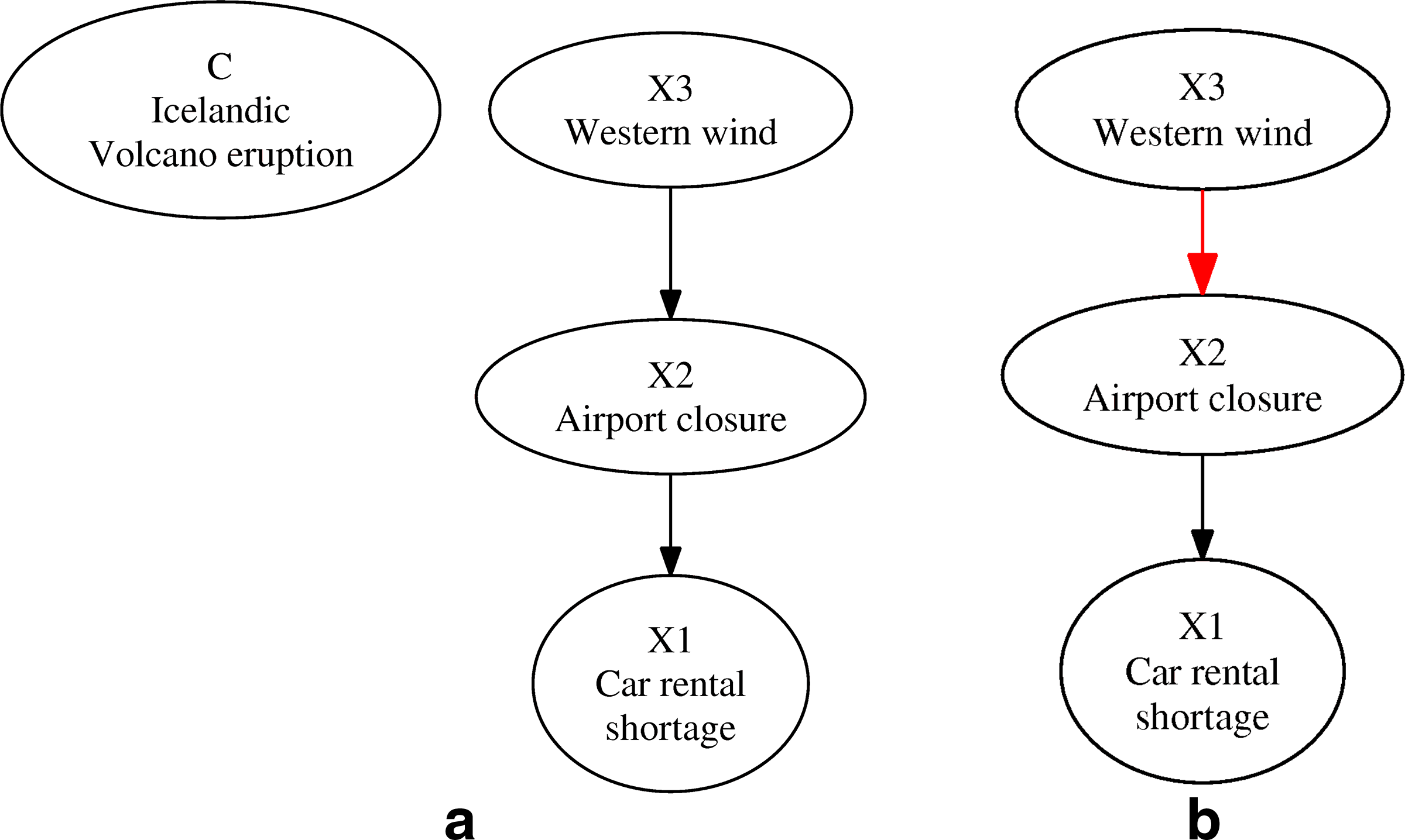
Figure 2 displays the joint probability mapping of our example, represented by a BNT. It is clear that the new edge, x ₃ → x ₂, which appears in the resulting network, suggests that this unique association has been discovered.

FIG. 2.

Bayesian Network representing the joint distribution mapping of X1, X2, X3, and the condition C. The edge x₃ → x₂ was retrieved using the BNT.

However, this case demonstrates the ambiguity encountered when trying to discover conditioned associations using BNT. The x ₃ → x ₂ association can result from an existing correlation between ( x ₃) and ( x ₂) in the general population and is not specific to the conditioned case, in which c=true. When this graph is the only source of information, there is no way to distinguish between background associations (in the general case) and conditioned associations (in the conditioned case).

This matter could be resolved by exploring the differences between the BNT without the condition variable and the BNT containing the condition variable. Yet in many cases, the proportion of the samples with a positive value of the condition variable may be large enough for the conditioned associations to appear in the BNT without the condition variable. In other cases, when the proportion of the samples with a positive condition value is small enough, the conditioned associations will not be discovered in the BNT with the condition variable. In fact, the former ambiguity was clearly visible in a simulation described later in this article.

Deforche et al. (2006) overcomes this issue by preexamining the candidate variables for the BNT and selecting variables that show significant correlation with the condition. This way the chance that background associations will arise is lowered; conversely, conditioned associations with variables that are not significantly correlated with the condition may be lost. In the above example, since Western wind ( x ₃) is not correlated with the volcanic eruption ( c ), ( x ₃) will not be used in our BNT; therefore, the x ₃ → x ₂ association will be lost.

Another drawback might be caused by the stochastic nature of searching the BNT model and its DAG structure. Reconstructing the BNT structure from given observational data requires searching through all possible models and looking for the model that maximizes the log-likelihood of the data. Since this problem is NP-Hard (Chickering et al., 2004), cases with more than a few variables require heuristic search methods (Friedman et al., 2000). Since prior causal knowledge is missing in many cases, our model search can result in structures that satisfy the observed statistical dependencies, but cannot accurately recover the underlying “real” structure or suggest an equivalent model that may hide the conditioned associations.

Consider the case displayed in Figure 3a, where an additional variable is added to our network: ash cloud ( x ₄). This DAG can be observationally equivalent (Pearl, 2009) DAGs (Fig. 3b) where the statistical dependencies between the variables (herein, d-separation [Pearl, 2009]) are still maintained, i.e., ( c ) and ( x ₂) are independent given ( x ₄). In the case displayed in Figure 3b, the causal relationship is obviously wrong.

FIG. 3.

Alternate Bayesian Network representation of our data. These networks maintain the d-separation criteria between the variables, though now the novel conditioned association (x₃ → x₂) should be searched within the whole connected component containing C.

This example shows the ambiguity faced when trying to draw conclusions concerning the conditioned association while exploring the graph structure of the BNT. In cases where the network structure is unknown, a single criterion cannot be applied in order to locate the conditioned associations, since we can alternate between two different graph structures that represent a single conditioned association.

This ambiguity affects the search procedure applied in order to locate the novel conditioned associations. To ensure that the conditioned association edges are covered by our search space, the edge directions should be ignored and the edges of the connected component containing the condition should be added to our search space. However, our search space will be greatly obscured by background association added to our result. Applying the methods described above, such as adding an activating variable (Pearl, 1993) to the condition variables, or removing the edges from the parents of the condition variable, while increasing the inference capabilities of the network, still does not eliminate the ambiguity regarding other variables.

Dependency networks

Heckerman et al. (2000) suggest a method that deals with some of the problems that arise, when interpreting a resultant BNT, especially the tight topology constraints, such as DAG, and the dependencies implied from the d-separation criteria.

This method iteratively regresses, using probabilistic decision trees. Each variable uses the rest of the model variables, and uses the prediction capabilities of the regressor variables as criteria for adding an edge between the regressor variables and the predicted variable. This method retains the “Markov Blanket” property of the BNT—given the parents' values for a network variable; it renders this variable independent of all other variables.

Dependency networks provide another advantage over other modeling methods: since the computation is done locally over the variable's immediate neighborhood, the computational effort is polynomial over the number of variables and, as such, more efficient.

Meinshausen et al. (2006) suggest a method for reconstructing the variables' graphical neighborhood using an estimation of Tibshirani's (1996) lasso method, applying penalty over the regression coefficients norm, and applying a zero value to coefficients with negligible prediction values. While regressing a variable using all the other variables as predictors. Non-zero coefficients will add an edge between the predictor and the predicted variables, that is, enabling a robust and computational efficient method for reconstructing a dependency network, especially in high dimensional cases.

Friedman et al. (2008) later enhance this model, suggesting an efficient exact solution to the lasso peer regression problem, using the Banerjee et al. (2008) blockwise coordinate descent approach. This method, herein graphical lasso, is demonstrated on cell signaling data from 11 different proteins.

Dependency networks efficiently solve the above problems, providing a straightforward interpretation and usage of a robust numerical mechanism. Yet the ambiguity between the background and conditioned associations still needs to be solved, since the condition variable is still part of the resulting network.

Current state of the art and the proposed method

The above sections display the inherent limitations of locating conditioned associations using BNT modeling, mainly the DAG structure that constrains the network structure and observational equivalency that may produce different graphical models for similar variable dependencies. Both limitations can cause the conditioned associations to appear far, or not on the path of the condition variable in the result graph, and so, largely increase the number of associations that need to be tested as candidates for conditioned associations.

Dependency networks and their recent adaptations solve this problem by addressing the local dependency neighborhood of the variable. Therefore, at least one of the conditioned association vertices should be a neighbor of the condition variable.

Yet, both Bayesian and dependency networks may identify associations that are independent of the condition (background associations). Since the background associations have the same topological features as conditioned associations, it is hard to discriminate between conditioned and non-conditioned associations, which results in a major increase in the search space.

We introduce a modification of the dependency network method, which obtains a graph containing only conditioned related associations.

We suggest a tool, based on an efficient and numerically robust implementation of ridge regression, which maps the associations of variables under the condition. These properties render it invariant to the proportion of the conditioned samples in the population. The resulting graph identifies the associations between variables that are correlated specifically under the condition variables, and so solving the ambiguity between associations in the general population (background associations) and conditioned associations.

2. IRR Method

We suggest a method that graphically maps conditioned associations between variables. Each association can be illustrated as a directed edge between the variables. The edges can be weighted according to the assumed prediction strength between the variables under the condition. The result will be a network structure (built as a directed graph) that will map the variable associations under the condition.

Exploring the network structure is done by regressing the condition variable using the remaining variables, observing the weight change of the regressor variables when omitting one, and then again regressing the condition variable by the remaining variables.

We will show that the weight change in the remaining variables is relative to their predictive value over the omitted variable under the condition.

Prediction capabilities of one variable by another, under the condition, can be used as a cue for conditioned association, which can later be tested separately by a simple hypothesis testing tool.

Defining the problem

Let \documentclass{aastex}\usepackage{amsbsy}\usepackage{amsfonts}\usepackage{amssymb}\usepackage{bm}\usepackage{mathrsfs}\usepackage{pifont}\usepackage{stmaryrd}\usepackage{textcomp}\usepackage{portland, xspace}\usepackage{amsmath, amsxtra}\pagestyle{empty}\DeclareMathSizes{10}{9}{7}{6}\begin{document} $$ S = \{x_1 , x_2 , \ldots x_n \}$$ \end{document} be a set of random binary variables (features), random binary variable c (condition), and a data sample set D, where each sample represents a vector for the value of \documentclass{aastex}\usepackage{amsbsy}\usepackage{amsfonts}\usepackage{amssymb}\usepackage{bm}\usepackage{mathrsfs}\usepackage{pifont}\usepackage{stmaryrd}\usepackage{textcomp}\usepackage{portland, xspace}\usepackage{amsmath, amsxtra}\pagestyle{empty}\DeclareMathSizes{10}{9}{7}{6}\begin{document} $$ x_1 , x_2 , \ldots x_n$$ \end{document} and their corresponding c value. Next, generate a graph (network) G = {V, E} where each node corresponds to a variable of \documentclass{aastex}\usepackage{amsbsy}\usepackage{amsfonts}\usepackage{amssymb}\usepackage{bm}\usepackage{mathrsfs}\usepackage{pifont}\usepackage{stmaryrd}\usepackage{textcomp}\usepackage{portland, xspace}\usepackage{amsmath, amsxtra}\pagestyle{empty}\DeclareMathSizes{10}{9}{7}{6}\begin{document} $$ \{x_1 , x_2 , \ldots x_n \}$$ \end{document} ; add an edge x_j → x_k , if the association { x_j , x_k } under the condition c is significantly better than in the general population. The direction of the edge is dependent upon the prediction direction between x_j and x_k if x_j can predict the value of x_k under the condition c, there will be an edge directed from x_j to x_k , and vice versa.

Selection or regularized regression method

In a classic regression problem, we want to find a weight set W that satisfies the equation: \documentclass{aastex}\usepackage{amsbsy}\usepackage{amsfonts}\usepackage{amssymb}\usepackage{bm}\usepackage{mathrsfs}\usepackage{pifont}\usepackage{stmaryrd}\usepackage{textcomp}\usepackage{portland, xspace}\usepackage{amsmath, amsxtra}\pagestyle{empty}\DeclareMathSizes{10}{9}{7}{6}\begin{document} \begin{align*}\leqslant\mathop{ \rm argmin} \limits_{w} E \left ( Y - \sum_{i = 1 \rightarrow n} w_i x_i \right ) ^2 \tag {1}\end{align*} \end{document}

In order to handle the problem of regressing variables with high covariance (typical of the problems explored by the Iterative Ridge Regression [IRR]), which cause instability when inverting the sample matrix, a statistical method called ridge regression, or Tikhonov regularization (Tychonoff and Arsenin, 1977) is utilized. This method adds a penalty over the weight vector norm. \documentclass{aastex}\usepackage{amsbsy}\usepackage{amsfonts}\usepackage{amssymb}\usepackage{bm}\usepackage{mathrsfs}\usepackage{pifont}\usepackage{stmaryrd}\usepackage{textcomp}\usepackage{portland, xspace}\usepackage{amsmath, amsxtra}\pagestyle{empty}\DeclareMathSizes{10}{9}{7}{6}\begin{document} \begin{align*}\mathop{ \rm argmin} \limits_{w} E \left ( Y - \sum_{i = 1 \rightarrow n} w_i x_i \right ) ^2 + \lambda \ \| W \| ^2 \tag {2}\end{align*} \end{document}

where the λ parameter stands for the ridge parameter.

Another method, called the lasso regularization, suggested by Tibshirani (1996), replaces the ridge regression's L2 norm penalty of the weight vector, with L1 norm penalty: \documentclass{aastex}\usepackage{amsbsy}\usepackage{amsfonts}\usepackage{amssymb}\usepackage{bm}\usepackage{mathrsfs}\usepackage{pifont}\usepackage{stmaryrd}\usepackage{textcomp}\usepackage{portland, xspace}\usepackage{amsmath, amsxtra}\pagestyle{empty}\DeclareMathSizes{10}{9}{7}{6}\begin{document} \begin{align*}\lambda \ \| W \| \ \ell 1\end{align*} \end{document}

While it also has an efficient solution of the weight vector, it also tends toward a zero value for negligible coefficients when using a large enough λ value.

As was recently suggested, the elastic nets (Zou and Hastie, 2005) use a mix of L2 and L1 regularization over the weight norm: \documentclass{aastex}\usepackage{amsbsy}\usepackage{amsfonts}\usepackage{amssymb}\usepackage{bm}\usepackage{mathrsfs}\usepackage{pifont}\usepackage{stmaryrd}\usepackage{textcomp}\usepackage{portland, xspace}\usepackage{amsmath, amsxtra}\pagestyle{empty}\DeclareMathSizes{10}{9}{7}{6}\begin{document} \begin{align*}\lambda ( ( 1 - \alpha ) \| W \| ^2 + \alpha \| W \| _{ \ell 1} )\end{align*} \end{document}

where the α parameter value determines whether the penalty leans toward L2 (which displays the ridge regression behavior) or L1 (lasso).

In their most recent article, Friedman et al. (2010) display a distinction between the above three regularization methods—ridge regression, lasso, and elastic nets—in regards to the effect of the weight change of regressor variables after omitting one of them.

Since the L2 norm penalty amplifies an uneven weight distribution, ridge regression tends to split the coefficient weight of the omitted variable between the highly correlated variables. Lasso, on the other hand, tends to pick one correlated variable to receive the weight of the omitted variable. Elastic-nets behavior depends on the value of the α parameter.

In our case, the inter-relations between the variables are more relevant than the precision of the model's prediction. Therefore, the ridge regression will be more suitable for our needs, while there is a need for a threshold value to filter the negligible interaction,

Iterative interaction discovery

Once the regularization method is chosen, the conditioned interactions are discovered while iterating over the model variables.

At the first stage, the regression of the condition variable will be done, using the variables in S: \documentclass{aastex}\usepackage{amsbsy}\usepackage{amsfonts}\usepackage{amssymb}\usepackage{bm}\usepackage{mathrsfs}\usepackage{pifont}\usepackage{stmaryrd}\usepackage{textcomp}\usepackage{portland, xspace}\usepackage{amsmath, amsxtra}\pagestyle{empty}\DeclareMathSizes{10}{9}{7}{6}\begin{document} \begin{align*}W^B = \mathop { \rm argmin} \limits_{w} E \left ( C - \sum_{x_i \in S} w_i x_i \right ) ^2 + \lambda \ \| W \| ^2 \tag {3}\end{align*} \end{document}

Later, in each iteration j, the values of variable x_j will be omitted from the samples' data, and the condition variable will again be predicted using the remaining variables: \documentclass{aastex}\usepackage{amsbsy}\usepackage{amsfonts}\usepackage{amssymb}\usepackage{bm}\usepackage{mathrsfs}\usepackage{pifont}\usepackage{stmaryrd}\usepackage{textcomp}\usepackage{portland, xspace}\usepackage{amsmath, amsxtra}\pagestyle{empty}\DeclareMathSizes{10}{9}{7}{6}\begin{document} \begin{align*}W^j = \mathop { \rm argmin} \limits_{w} E \left ( C - \sum_{x_i \in S / x_j} w_i x_i \right ) ^2 + \lambda \ \| W \| ^2 \tag {4}\end{align*} \end{document}

This results in a new set of weights for the remaining features, W^j, which will be compared with the original set of weights. The weight difference of each feature can be computed: ΔW^j = W^B − W^j

As proved in Appendix 7c, ΔW^j is the coefficients vector that gives the best regularized estimation of \documentclass{aastex}\usepackage{amsbsy}\usepackage{amsfonts}\usepackage{amssymb}\usepackage{bm}\usepackage{mathrsfs}\usepackage{pifont}\usepackage{stmaryrd}\usepackage{textcomp}\usepackage{portland, xspace}\usepackage{amsmath, amsxtra}\pagestyle{empty}\DeclareMathSizes{10}{9}{7}{6}\begin{document} $$ W_j^B x_j$$ \end{document} . \documentclass{aastex}\usepackage{amsbsy}\usepackage{amsfonts}\usepackage{amssymb}\usepackage{bm}\usepackage{mathrsfs}\usepackage{pifont}\usepackage{stmaryrd}\usepackage{textcomp}\usepackage{portland, xspace}\usepackage{amsmath, amsxtra}\pagestyle{empty}\DeclareMathSizes{10}{9}{7}{6}\begin{document} \begin{align*}\Delta W^j = \mathop { \rm argmin} \limits_{w} E \left ( W_j^B x_j - \sum_{x_i \in S / x_j} w_ix_i \right ) ^2 + \lambda \ \| W^B - W \| ^2 \tag {5}\end{align*} \end{document}

At this point, the benefits of ridge regression come in hand. The best estimation of \documentclass{aastex}\usepackage{amsbsy}\usepackage{amsfonts}\usepackage{amssymb}\usepackage{bm}\usepackage{mathrsfs}\usepackage{pifont}\usepackage{stmaryrd}\usepackage{textcomp}\usepackage{portland, xspace}\usepackage{amsmath, amsxtra}\pagestyle{empty}\DeclareMathSizes{10}{9}{7}{6}\begin{document} $$ W_j^B x_j$$ \end{document} is biased towards the selection of ΔW_j, which evenly distribute the weights between variables that are correlated with x_j under C.

For instance, if x ₁ and x ₂ are fully correlated with x_j , the result will be \documentclass{aastex}\usepackage{amsbsy}\usepackage{amsfonts}\usepackage{amssymb}\usepackage{bm}\usepackage{mathrsfs}\usepackage{pifont}\usepackage{stmaryrd}\usepackage{textcomp}\usepackage{portland, xspace}\usepackage{amsmath, amsxtra}\pagestyle{empty}\DeclareMathSizes{10}{9}{7}{6}\begin{document} $$ [ \Delta W^j ] _1 = [ \Delta W^j ] _2 = \frac{1}{2}$$ \end{document} , while in L1 norm penalty, the result may be [ΔW_j]₁ = 1 and [ΔW_j]₁ = 0, or vice versa.

In this case, one can expect all of the variables that highly correlate with x_j under c, to receive significant value in the corresponding ΔW^j index.

Therefore, each element i in ΔW^j represents the prediction level of x_j using x_i under the condition c. This element can be used as a cue for the conditioned association level between x_i and x_j .

If [ΔW^j]i passes a known threshold t, the association x_j → x_k can be tested using an independent χ² test, whether it is statistically significant under the condition c. The X² test results are adjusted for false discovery rate using the Hochberg-Benjamini correction (Benjamini and Hochberg, 1995).

Passing both criteria, an edge x_j → x_k will be added to our graph G.

See Appendix (sections 7a and 7b) for pseudo code and demonstration of the method.

Complexity of the IRR algorithm

Since the IRR algorithm uses both ridge regression and χ² test, both have many robust and efficient implementations, its calculation time is a linear function over the sample size.

Overall, using an N size variable set and an M size sample set, the IRR regresses the sample set N times, then tests again within the set all of the N variables for significant associations.

In this case, the IRR's asymptotic complexity is O(N²M).

3. Comparing the IRR Algorithm with BNT

Herein is a performance comparison of the IRR algorithm with the state-of-the art BNT algorithm. Both algorithms try to locate a priori induced associations between variables that correlate under a condition.

Data set construction

The sample set contains 1000 samples with 20 variables. Each variable can hold a binary value of − 1 or 1.

Each sample is assigned with a binary condition value; the total size of the condition vector is 1000 samples. All sample values were initialized to −1, afterwards 0.2 of the samples had their values inversed to simulate background noise.

Out of the 20 variables, four variables were randomly selected to hold the conditioned pattern – their values will be correlated under the condition and random otherwise.

Out of the condition vector, a predefined ratio (0.8) of the samples was set as a condition, and their values were set to 1. Out of the conditioned samples, a predefined ratio (0.2) was randomly selected to hold the pattern. These samples will have a positive (1) value in the conditioned pattern variables.

After the construction of the sample set, sampling noise was induced by inversing the values of a predefined ratio (noise level) of the sample set.

Simulation overview

Both the IRR and the BNT algorithms were used to extract the conditioned pattern variables. We used the BNT Matlab package of Murphy (2001) for BNT construction. The BNT was constructed using the K2 algorithm (Cheng et al., 1997) that outperformed other network construction algorithms (Leray and Francois, 2004).

As described above, the BNT result DAG was searched for the connected component containing the condition variable. All the variables in this connected component (ignoring edge directions) were tested as the result pattern.

The BNT and the IRR result patterns were tested against the induced pattern and scored using the Jaccard Index. For each noise level, 100 independent simulation executions were performed, and the mean and standard deviation of the Jaccard score were used as a basis for performance comparison between the IRR and the BNT (see exact simulation details in Appendix 7d).

Results

See Table 1 and Figure 4.

FIG. 4.

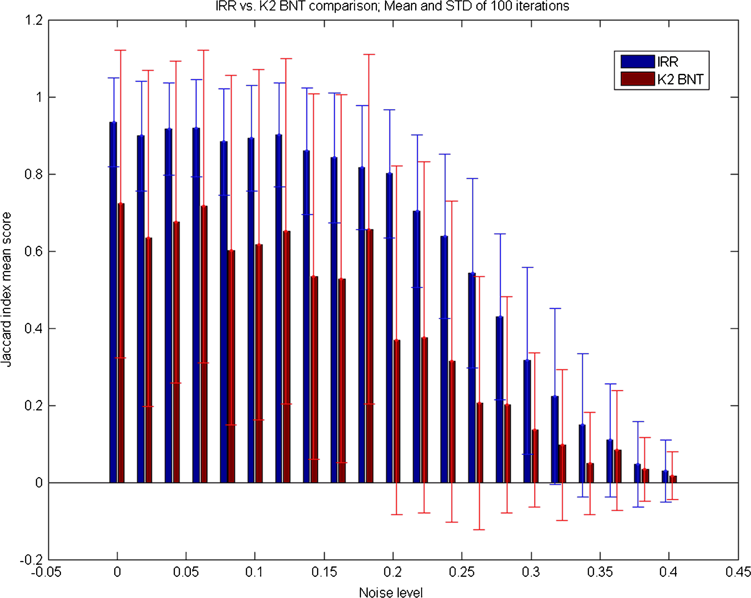
Graphic representation of the Jaccard index scoring mean and STD of the IRR and Bayesian Network K2 algorithms, over 100 iterations. The IRR algorithm significantly outperforms the Bayesian Network K2 algorithm (p < 0.01). The STD values show more stable performance by the IRR as compared with the K2 algorithm.

Table 1.

Mean Jaccard Index Scoring Over 100 Iterations of the IRR and Bayesian Network K2 Algorithms Along Various Noise Levels

Noise level	IRR	K2
0	0.9340	0.7220
0.02	0.8980	0.6327
0.04	0.9163	0.6750
0.06	0.9180	0.7153
0.08	0.8828	0.6020
0.1	0.8923	0.6173
0.12	0.9012	0.6504
0.14	0.8593	0.5330
0.16	0.8418	0.5280
0.18	0.8160	0.6558
0.2	0.8001	0.3687
0.22	0.7030	0.3755
0.24	0.6382	0.3135
0.26	0.5423	0.2052
0.28	0.4298	0.2015
0.3	0.3153	0.1360
0.32	0.2223	0.0965
0.34	0.1480	0.0492
0.36	0.1093	0.0827
0.38	0.0470	0.0329
0.4	0.0295	0.0170

The comparison results

The simulation results show that the IRR performs well when trying to locate conditioned patterns in data that have up to 25% noisy (i.e., reversed) values. At these noise levels, the IRR significantly (p < 0.01) outperforms known state-of-the-art algorithms such as the K2 BNT algorithm.

These results emphasize the effect of association ambiguity of the BNT, as shown in the following simulation case:

In this case, a 4 sized pattern that includes variable numbers 1, 16, 17, and 20 was induced to a 20 random variables data set. These variables associate only under the condition; otherwise, they are randomly correlated.

Figure 5 shows that the IRR result is a fully connected graph, which includes the pattern variables. The BNT graph, which by nature is a DAG, contains the pattern variables but also two other variables (var12 and var15) that were randomly associated with the pattern variables, regardless of the condition.

FIG. 5.

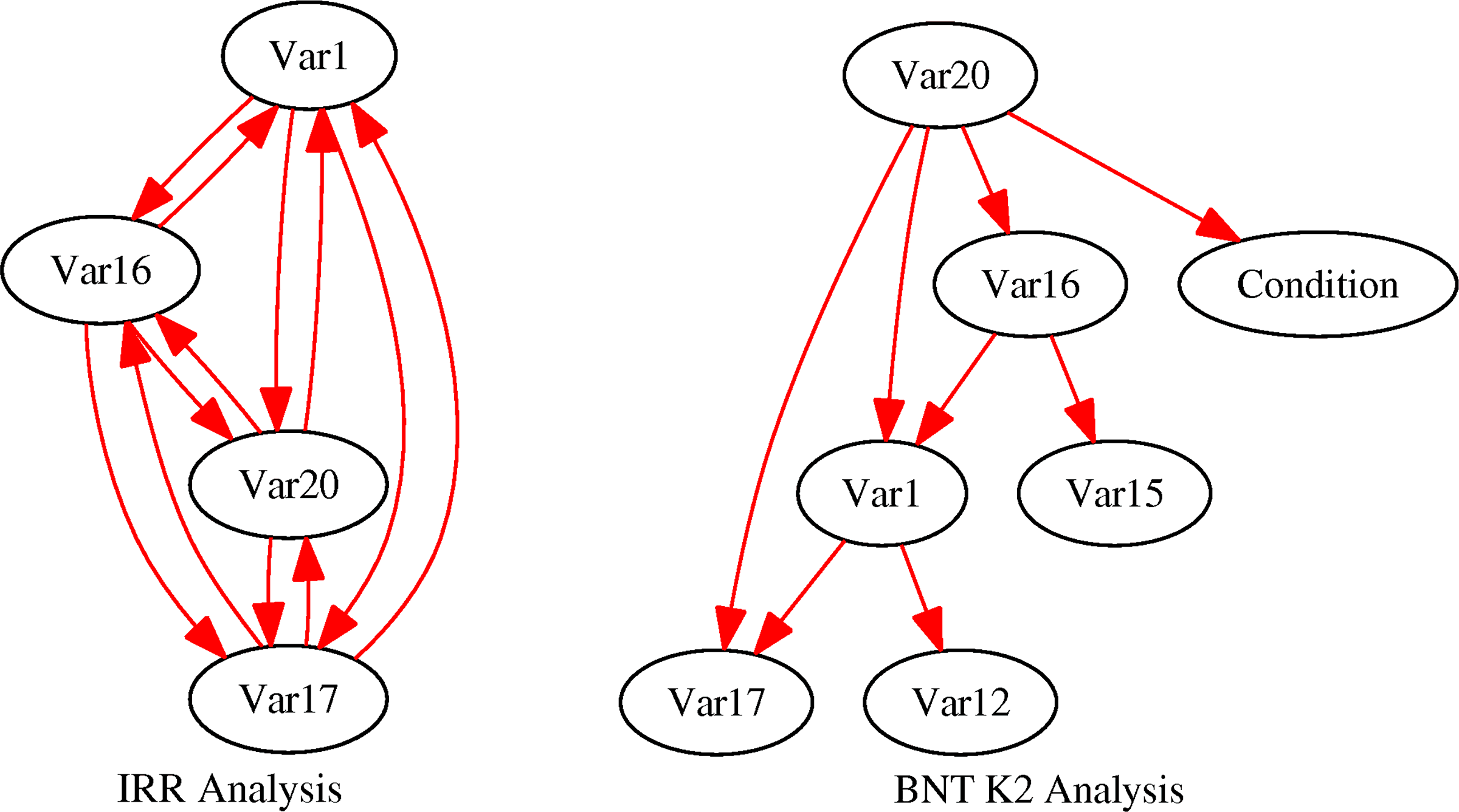
Graphical result of pattern locating. The pattern contains four variables (Var1, Var16, Var17, and Var20) in a 20 random variables data set. The IRR has fully located the induced pattern, while the BNT has also located two randomly correlated variables (Var12 and Var15), not associated in the pattern under the condition.

As described before, we can only assume about the conditional nature of the BNT result by exploring the connected component of the graph containing the condition, and ignoring the direction of the edges, thus including variables 12 and 15 in the suggested pattern result.

In this case, the Jaccard index score of the IRR graph will be 1 (fully compatible with the pattern), while the BNT result will be 0.67.

4. Application of the IRR for Prediction of Human Immunodeficiency Virus (HIV) Resistance Mutation Patterns

We used IRR to explore patterns of HIV RNA mutations that emerge in HIV-infected people after the initiation of antiretroviral drug treatment. These mutations, termed drug-resistant mutations, are preferentially selected because they render the virus resistant to the drugs admitted. In fact, this was the trigger for the development of IRR in the first place.

In most cases, the treatment is targeted to interfere with the activity of specific HIV proteins, such as viral protease, reverse-transcriptase and integrase. The mutations occur in parts of the viral RNA sequences that map into the protein active sites upon translation. These are the sites that are affected by the HIV treatment. Characterization of the associations between resistance mutations and treatment regimens can be beneficial in the selection and optimization of treatment. It can be used to predict the appearance of resistance mutations or to assess the functional behavior of the mutant protein and reveal interactions among the drugs and among different coexisting mutations.

Deforche et al. (2006) have explored the interactions between resistance mutations using BNT modeling. Their data set contained amino acid samples of the protease site from HIV patients and their treatment history (focusing specifically on the protease inhibitor [PI] Nelfinavir [NFV]). First, χ² test was applied to identify mutations that significantly correlated with the treatment. A new data set was then created, where the presence/absence of a given mutation in each sample was represented by the Boolean value of a variable assigned to this mutation. An additional variable was assigned to the NFV treatment status of this sample.

BNT modeling was used to explore associations between the variables described above. The resultant network recovered some of the known interactions between the NFV-induced mutations. It also pointed to new associations that were later found to be biologically meaningful.

We will briefly describe the application of IRR to the same biological process using our own data.

Data and method

A total of 1745 sample protease sequences were obtained from the depository of the National HIV Reference Laboratory (NHRL): 1261 samples were of individuals infected with subtype-C HIV, of which 170 were treated with NFV, and 454 samples were of subtype-B, of which 29 patients were treated with NFV.

Using IRR, we separately analyzed each subtype's samples, since C and B subtypes display different resistance mutation patterns (Grossman et al., 2004; Kantor et al., 2005; Rhee et al., 2006).

For each of the two subtypes, the amino acid sequences were compared to the subtype consensus sequence (that is, the sequence that is the best representative of the wild-type virus). The subtype consensus sequences were equal in samples from drug-naive HIV carriers and in the general sample population, reflecting the fact that variants constitute a small minority in the sequence population. After the consensus comparison, a mutations variable set was established by including every diversion from consensus that occurred at least twice

For each mutation, a binary variable was created, indicating for each sample whether the mutation appeared in that sample (positive value, set to + 1) or not (−1). Similarly, the condition variable binary value indicates the NFV treatment status for each sample.

A binary frequency matrix of the mutation variables and the condition variable over the sample population was used as input for the IRR algorithm.

The IRR algorithm used a value of 50 as the ridge parameter and p < 0.05 as the χ² test significance range.

Results

Graphical representations of the HIV mutation data constructed via IRR are displayed in Figure 6a (subtype B analysis) and 6b (subtype C analysis). Associations that showed exceptionally significant χ² scoring (p < 0.00000) and IRR scoring of >0.01 are marked by red edges.

FIG. 6.

IRR graphical result of amino acid mutations associations found in subtype B (a) and subtype C (b) HIV protease sequences, conditioned by Nelfinavir (NFV) treatment. Red edges suggest exceptionally significant associations with high IRR and X² scoring. Edge directions are such that the presence of the edge source will increase the probability of the edge target.

A detailed comparison with previously established results and a discussion of the potential significance of new, previously unknown associations is in preparation and will be published (Bar-Yaakov et al., 2011). Briefly, out of the 31 mutations in the IRR-generated networks, 13 have been previously identified as resistance mutations. The IRR network contains several directed paths that match known resistance mutation pathways. In addition, the IRR network shared 24 mutations and a number of pathways with the BNT generated through the analysis of Deforche et al. (2006). Importantly, the IRR method revealed novel associations, such as V15I-D30N, that are biologically plausible and that provide new insights into the mechanisms of drug-resistance development.

Our results display some inconsistencies with previous publications. These and implications regarding limitations of the method and possible remedies are discussed in more detail in elsewhere (Bar-Yaakov et al., 2011).

5. Conclusion

This article introduced IRR, a modification of the dependency network method, which produces a directed graph containing only condition-related associations. We have described a robust and computationally efficient estimator algorithm used to uncover such a network.

We showed that the IRR algorithm performs better than the current state-of-the-art BNT when the purpose is to identify conditioned associations.

We also briefly describe, here and in a forthcoming publication, a real-life application of the IRR method to the analysis of HIV mutation patterns that emerge in HIV-infected patients treated with a particular antiretroviral drug. We have demonstrated that our method can recover, from a pool of viral sequences, known associations of such treatment with selected resistance mutations as well as documented associations between different mutations. Moreover, the IRR method revealed novel associations that are statistically significant and biologically plausible.

6. Appendix

For IRR pseudo code and detailed demonstration of the IRR algorithm, please refer to www.cs.tau.il/∼nin.

Analytical proof of the IRR method

Given a random variable set \documentclass{aastex}\usepackage{amsbsy}\usepackage{amsfonts}\usepackage{amssymb}\usepackage{bm}\usepackage{mathrsfs}\usepackage{pifont}\usepackage{stmaryrd}\usepackage{textcomp}\usepackage{portland, xspace}\usepackage{amsmath, amsxtra}\pagestyle{empty}\DeclareMathSizes{10}{9}{7}{6}\begin{document} $$ S = \{x_1 , x_2 , \ldots x_n \}$$ \end{document} and a condition variable c, denote W^B as the basis weight vector of ridge regressing c using S: \documentclass{aastex}\usepackage{amsbsy}\usepackage{amsfonts}\usepackage{amssymb}\usepackage{bm}\usepackage{mathrsfs}\usepackage{pifont}\usepackage{stmaryrd}\usepackage{textcomp}\usepackage{portland, xspace}\usepackage{amsmath, amsxtra}\pagestyle{empty}\DeclareMathSizes{10}{9}{7}{6}\begin{document} \begin{align*}W^B = \mathop { \rm argmin} \limits_{w} E \left ( c - \sum_{x_i \in S} w_i x_i \right ) ^2 + \lambda \ \| W \| ^2\end{align*} \end{document}

Let W^j be the resulting weight vector, after the ridge regression of c using S excluding x_j: \documentclass{aastex}\usepackage{amsbsy}\usepackage{amsfonts}\usepackage{amssymb}\usepackage{bm}\usepackage{mathrsfs}\usepackage{pifont}\usepackage{stmaryrd}\usepackage{textcomp}\usepackage{portland, xspace}\usepackage{amsmath, amsxtra}\pagestyle{empty}\DeclareMathSizes{10}{9}{7}{6}\begin{document} \begin{align*}W^j = \mathop { \rm argmin} \limits_{w} E \left ( c - \sum_{x_i \in S / x_j} w_i x_i \right ) ^2 + \lambda \ \| W \| ^2\end{align*} \end{document}

In the case where \documentclass{aastex}\usepackage{amsbsy}\usepackage{amsfonts}\usepackage{amssymb}\usepackage{bm}\usepackage{mathrsfs}\usepackage{pifont}\usepackage{stmaryrd}\usepackage{textcomp}\usepackage{portland, xspace}\usepackage{amsmath, amsxtra}\pagestyle{empty}\DeclareMathSizes{10}{9}{7}{6}\begin{document} $$ W_j^B \neq 0$$ \end{document} , i.e., x_j has significant part in estimating c, we receive: \documentclass{aastex}\usepackage{amsbsy}\usepackage{amsfonts}\usepackage{amssymb}\usepackage{bm}\usepackage{mathrsfs}\usepackage{pifont}\usepackage{stmaryrd}\usepackage{textcomp}\usepackage{portland, xspace}\usepackage{amsmath, amsxtra}\pagestyle{empty}\DeclareMathSizes{10}{9}{7}{6}\begin{document} \begin{align*}E \left( c - \sum_{x_i \in S} W_j^B x_j \right)^2 + \lambda \| W^B \|^2 < E \left( c - \sum_{x_i \in S / x_j} W^j {}_ix_i \right)^2 + \lambda \| W^j \|^2 \end{align*} \begin{align*}\Delta W^j = \mathop { \rm argmin} \limits_{w} E \left ( W_j^B x_j - \sum_{x_i \in S / x_j} w_i x_i \right ) ^2 + \lambda \ \| W^B - W \| ^2\end{align*} \end{document}

Lemma. Denote ΔW^j to be the weight difference between the two results: ΔW^j = W^B − W^j. We wish to prove that ΔW^j is the coefficients vector that gives the best estimation of \documentclass{aastex}\usepackage{amsbsy}\usepackage{amsfonts}\usepackage{amssymb}\usepackage{bm}\usepackage{mathrsfs}\usepackage{pifont}\usepackage{stmaryrd}\usepackage{textcomp}\usepackage{portland, xspace}\usepackage{amsmath, amsxtra}\pagestyle{empty}\DeclareMathSizes{10}{9}{7}{6}\begin{document} $$ W_j^B x_j$$ \end{document} , while maintaining the regularization expression small:

\documentclass{aastex}\usepackage{amsbsy}\usepackage{amsfonts}\usepackage{amssymb}\usepackage{bm}\usepackage{mathrsfs}\usepackage{pifont}\usepackage{stmaryrd}\usepackage{textcomp}\usepackage{portland, xspace}\usepackage{amsmath, amsxtra}\pagestyle{empty}\DeclareMathSizes{10}{9}{7}{6}\begin{document} \begin{align*} E \left ( W_j^B x_j - \sum_{x_i \in S / x_j} \widetilde{W}^{\jmath}_{\imath} x_i \right ) ^2 + \lambda \ \| W^B - \widetilde{W}^{ \jmath} \| ^2 < E \left ( W_j^B x_j - \sum_{x_i \in S / x_j} \Delta W_i^j x_i \right ) ^2 + \lambda \ \| W^B - \Delta W^j \| ^2 \end{align*} \end{document}

Proof. Suppose there is an alternative set of weights: \documentclass{aastex}\usepackage{amsbsy}\usepackage{amsfonts}\usepackage{amssymb}\usepackage{bm}\usepackage{mathrsfs}\usepackage{pifont}\usepackage{stmaryrd}\usepackage{textcomp}\usepackage{portland, xspace}\usepackage{amsmath, amsxtra}\pagestyle{empty}\DeclareMathSizes{10}{9}{7}{6}\begin{document} $$ \widetilde{W}^{ \jmath} \neq \Delta W^j$$ \end{document} that offers better regularized estimation of \documentclass{aastex}\usepackage{amsbsy}\usepackage{amsfonts}\usepackage{amssymb}\usepackage{bm}\usepackage{mathrsfs}\usepackage{pifont}\usepackage{stmaryrd}\usepackage{textcomp}\usepackage{portland, xspace}\usepackage{amsmath, amsxtra}\pagestyle{empty}\DeclareMathSizes{10}{9}{7}{6}\begin{document} $$ W_j^B x_j$$ \end{document} than ΔW^j, hence:

\documentclass{aastex}\usepackage{amsbsy}\usepackage{amsfonts}\usepackage{amssymb}\usepackage{bm}\usepackage{mathrsfs}\usepackage{pifont}\usepackage{stmaryrd}\usepackage{textcomp}\usepackage{portland, xspace}\usepackage{amsmath, amsxtra}\pagestyle{empty}\DeclareMathSizes{10}{9}{7}{6}\begin{document} \begin{align*} E \left( W_j^B x_j - \sum_{x_i \in S / x_j} (\widetilde{\Delta W}^{ \jmath}_{ \imath} + \Delta W_i^j ) x_i \right)^2 + \lambda \ \| W^B - \widetilde{W}^{ \jmath} \| ^2 < E \left( W_j^B x_j - \sum_{x_i \in S / x_j} \Delta W_i^j x_i \right)^2 + \lambda \ \| W^B - \Delta W^j \|^2 \end{align*} \end{document}

Denote \documentclass{aastex}\usepackage{amsbsy}\usepackage{amsfonts}\usepackage{amssymb}\usepackage{bm}\usepackage{mathrsfs}\usepackage{pifont}\usepackage{stmaryrd}\usepackage{textcomp}\usepackage{portland, xspace}\usepackage{amsmath, amsxtra}\pagestyle{empty}\DeclareMathSizes{10}{9}{7}{6}\begin{document} $$ \widetilde{ \Delta W}^{ \jmath}$$ \end{document} as their weight difference: \documentclass{aastex}\usepackage{amsbsy}\usepackage{amsfonts}\usepackage{amssymb}\usepackage{bm}\usepackage{mathrsfs}\usepackage{pifont}\usepackage{stmaryrd}\usepackage{textcomp}\usepackage{portland, xspace}\usepackage{amsmath, amsxtra}\pagestyle{empty}\DeclareMathSizes{10}{9}{7}{6}\begin{document} $$ \widetilde{ \Delta \rm W}^{ \j} = \widetilde{\rm W}^{ \j} - \Delta {\rm W^j}$$ \end{document} . After decomposing \documentclass{aastex}\usepackage{amsbsy}\usepackage{amsfonts}\usepackage{amssymb}\usepackage{bm}\usepackage{mathrsfs}\usepackage{pifont}\usepackage{stmaryrd}\usepackage{textcomp}\usepackage{portland, xspace}\usepackage{amsmath, amsxtra}\pagestyle{empty}\DeclareMathSizes{10}{9}{7}{6}\begin{document} $$ \widetilde{W}^{ \jmath}$$ \end{document} : \documentclass{aastex}\usepackage{amsbsy}\usepackage{amsfonts}\usepackage{amssymb}\usepackage{bm}\usepackage{mathrsfs}\usepackage{pifont}\usepackage{stmaryrd}\usepackage{textcomp}\usepackage{portland, xspace}\usepackage{amsmath, amsxtra}\pagestyle{empty}\DeclareMathSizes{10}{9}{7}{6}\begin{document} \begin{align*} E \left( W_j^B x_j - \sum_{x_i \in S / x_j} \Delta W_i^j x_i + \sum_{x_i \in S / x_j} \widetilde{ \Delta W}_{ \imath}^{ \jmath}x_i \right)^2 + \lambda \ \| W^B - \Delta W^j + \widetilde{ \Delta W}^{ \jmath} \| ^2 // & \qquad < E \left( W_j^B x_j - \sum_{x_i \in S / x_j} \Delta W_i^j x_i \right) ^2 + \lambda \ \| W^B - \Delta W^j \| ^2 \end{align*} \end{document}

Hence: \documentclass{aastex}\usepackage{amsbsy}\usepackage{amsfonts}\usepackage{amssymb}\usepackage{bm}\usepackage{mathrsfs}\usepackage{pifont}\usepackage{stmaryrd}\usepackage{textcomp}\usepackage{portland, xspace}\usepackage{amsmath, amsxtra}\pagestyle{empty}\DeclareMathSizes{10}{9}{7}{6}\begin{document} \begin{align*} E \left( c - \sum_{x_i \in S} W_i^B x_i \right) ^2 + \lambda \ \| W^B \| ^2 < E \left( c - \sum_{x_i \in S / x_j}W^j {}_ix_i \right) ^2 + \lambda \ \| W^j \| ^2 \end{align*} \end{document}

Since: \documentclass{aastex}\usepackage{amsbsy}\usepackage{amsfonts}\usepackage{amssymb}\usepackage{bm}\usepackage{mathrsfs}\usepackage{pifont}\usepackage{stmaryrd}\usepackage{textcomp}\usepackage{portland, xspace}\usepackage{amsmath, amsxtra}\pagestyle{empty}\DeclareMathSizes{10}{9}{7}{6}\begin{document} \begin{align*} E \left( c - \sum_{x_i \in S / x_j} W_i^B x_i + W_j^B x_j \right) ^2 + \lambda \ \| W^B \| ^2 < E \left( c - \sum_{x_i \in S / x_j} W_i^B x_i + \sum_{x_i \in S / x_j} \Delta W_{ i}^j x_i \right) ^2 + \lambda \| W^j \| ^2 \end{align*} \end{document}

After decomposing: \documentclass{aastex}\usepackage{amsbsy}\usepackage{amsfonts}\usepackage{amssymb}\usepackage{bm}\usepackage{mathrsfs}\usepackage{pifont}\usepackage{stmaryrd}\usepackage{textcomp}\usepackage{portland, xspace}\usepackage{amsmath, amsxtra}\pagestyle{empty}\DeclareMathSizes{10}{9}{7}{6}\begin{document} \begin{align*} E \left( c - \sum_{x_i \in S / x_j} W_i^B x_i + \sum_{x_i \in S / x_j} \Delta W_i^j x_i + \sum_{x_i \in S / x_j} \widetilde{ \Delta W}_{ \imath}^{ \jmath} x_i \right)^2 + \lambda \ \| W^B - \Delta W^j + \widetilde{ \Delta W}^{ \jmath} \| ^2 // & \qquad < E \left( c - \sum_{x_i \in S / x_j} W_i^B x_i + \sum_{x_i \in S / x_j} \Delta W_i^j x_i \right) ^2 + \lambda \ \| W^B - \Delta W^j \|^2 \end{align*} \end{document}

Since we have a better regularized estimation for \documentclass{aastex}\usepackage{amsbsy}\usepackage{amsfonts}\usepackage{amssymb}\usepackage{bm}\usepackage{mathrsfs}\usepackage{pifont}\usepackage{stmaryrd}\usepackage{textcomp}\usepackage{portland, xspace}\usepackage{amsmath, amsxtra}\pagestyle{empty}\DeclareMathSizes{10}{9}{7}{6}\begin{document} $$ { \rm W}^{ \rm B} {}_{ \rm j}{ \rm x}_{ \rm j}$$ \end{document} : \documentclass{aastex}\usepackage{amsbsy}\usepackage{amsfonts}\usepackage{amssymb}\usepackage{bm}\usepackage{mathrsfs}\usepackage{pifont}\usepackage{stmaryrd}\usepackage{textcomp}\usepackage{portland, xspace}\usepackage{amsmath, amsxtra}\pagestyle{empty}\DeclareMathSizes{10}{9}{7}{6}\begin{document} \begin{align*} E \left( c - \sum_{x_i \in S / x_j} W_i^j x_i + \sum_{x_i \in S / x_j} \widetilde{ \Delta W}_{ \imath}^{ \jmath} x_i \right) ^2 + \lambda \ \| W^j + \widetilde{ \Delta W}^{ \jmath} \| ^2 < E \left( c - \sum_{x_i \in S / x_j} W^j {}_ix_i \right) ^2 + \lambda \ \| W^j \| ^2 \end{align*} \end{document}

Therefore, it can use \documentclass{aastex}\usepackage{amsbsy}\usepackage{amsfonts}\usepackage{amssymb}\usepackage{bm}\usepackage{mathrsfs}\usepackage{pifont}\usepackage{stmaryrd}\usepackage{textcomp}\usepackage{portland, xspace}\usepackage{amsmath, amsxtra}\pagestyle{empty}\DeclareMathSizes{10}{9}{7}{6}\begin{document} $$ \widetilde{ \Delta W}^{ \jmath}$$ \end{document} for better minimization of the condition variable estimation without using x_j: \documentclass{aastex}\usepackage{amsbsy}\usepackage{amsfonts}\usepackage{amssymb}\usepackage{bm}\usepackage{mathrsfs}\usepackage{pifont}\usepackage{stmaryrd}\usepackage{textcomp}\usepackage{portland, xspace}\usepackage{amsmath, amsxtra}\pagestyle{empty}\DeclareMathSizes{10}{9}{7}{6}\begin{document} \begin{align*} E \left( c - \sum_{x_i \in S / x_j} W_i^j x_i + \sum_{x_i \in S / x_j} \widetilde{\Delta W}_{\imath}^{\jmath} x_i \right)^2 + \lambda \ \| W^j + \widetilde{\Delta W}^{\jmath} \|^2 < E \left( c - \sum_{x_i \in S / x_j} W^j_i x_i \right)^2 + \lambda \ \| W^j \| ^2\end{align*} \end{document}

And this contradicts with the argmin property of W^j. ▪

In the above procedure, we have proved that by simple reduction of W^j from W^B we receive the best regularized estimation of the omitted variable by its co-variables.

Exact details of the IRR—BNT simulation

(A) Data simulation

(1) Parameters

(a) Number of features—N

(b) Number of samples—M

(d) Pattern description

(i) Pattern size—number of features in the pattern.

(ii) Pattern-condition ratio—the ratio of the conditioned samples which contains the pattern.

(e) Background noise level—ratio of random data members which have positive value (before pattern induction).

(f) Sampling noise level—ratio of random data members, which will have their value inverted.

(2) Data creation

(a) Allocate an N by M data matrix (samples).

(b) Allocate an M size vector (condition vector).

(d) Randomly select cells out of the sample's matrix, until selecting total cells ratio of background noise level. Inverse their value to 1.

(e) Randomly select cells out of the condition vector, until selecting an amount of cells corresponding to the condition ratio multiplied by the samples set size. These are the condition indices, Inverse their value to 1.

(f) Pattern induction

(i) Randomly select total of pattern size indices out of the features indices. These are the pattern indices.

(ii) Randomly select samples, until reaching total of (pattern-condition ratio * size of condition indices), which their corresponding indices in the condition vector are positive. These are the conditioned samples associated with the condition vector.

(iii) Change the values of the conditioned samples in the pattern indices to 1.

(g) Sampling noise induction

(i) Randomly select values until reaching a ratio of sampling noise level out of the samples values, and inverse their values.

(B) Single simulation execution

(1) IRR execution and scoring

(a) Use the sample matrix and the condition vector as an input to the IRR algorithm.

(b) IRR result is the estimated conditioned pattern; use Jaccard Index to evaluate the similarity between the original induced pattern and the estimated IRR result pattern.

(2) BNT execution and scoring

(a) We used the BNT package (Murphy, 2001) for executing a Bayesian network analysis over the simulated data.

(b) We compared the IRR with the K2 Bayesian network algorithms (Cheng et al., 1997), showed to outperform or match other BNET algorithms (Leray and Francois, 2004)

(c) Input for the BN was created by concatenating the sample matrix and the condition vector—the condition vector becomes another feature in the sample features.

(d) We used the DAG result of the Bayesian Network Power Constructor (BNPC) algorithm (Cooper and Herskovits, 1992), for topological sorting used to deduct the variable order, needed as an input for the K2 algorithm.

(e) The scoring was done by searching the connected component of the DAG result that contains the condition feature.

(f) We assemble a variable set containing the variables in the connected component.

(g) The set is regarded as the result estimated pattern of the algorithm.

(h) We use Jaccard Index to evaluate the similarity between the original induced pattern and the estimated BNT result pattern.

(1) In each comparison iteration, we simulated an input data matrix with parameters values as follows

(a) Number of features—N = 20

(b) Number of samples—M = 1000

(d) Single pattern induced

(i) Pattern size = 4

(ii) Pattern-condition ratio = 0.2.

(e) Background noise level = 0.2

(f) Sampling noise level = variable across the simulation

(2) We used the simulated data as an input to the IRR, BNPC, and K2 algorithms.

(3) For each set of parameters, we used 100 executions to get an average score on each sampling noise level.

Footnotes

Disclosure Statement

No competing financial interests exist.

References

Banerjee

, Ghaoui

L.E.

, d'Aspremont

2008. Model selection through sparse maximum likelihood estimation for multivariate Gaussian or binary data. J Mach. Learn. Res., 9:485–516.

Bar-Yaakov

, Intrator

, Grossman

2011. Interactions among PI-induced resistance mutations revealed by iterative ridge regression (in press).

Benjamini

, Hochberg

1995. Controlling the false discovery rate: a practical and powerful approach to multiple testing. J. R. Stat. Soc. B, 57:289–300.

Cheng

, Bell

D.A.

, Liu

1997. An algorithm for Bayesian belief network construction from data. Proc. AI STAT, 97:83–90.

Chickering

D.M.

, Heckerman

, Meek

2004. Large-sample learning of Bayesian networks is NP-hard. J. Mach. Learn. Res., 5:1287–1330.

Cooper

, Herskovits

1992. A Bayesian method for the induction of probabilistic networks from data. Mach. Learn., 9:309–347.

Deforche

, Silander

, Camacho

et al. 2006. Analysis of HIV-1 pol sequences using Bayesian networks: implications for drug resistance. Bioinfomatics, 22:2975–2979.

Edwards

D.M.

2000. Introduction to Graphical Modelling, 2nd. Springer: New York.

Friedman

, Linial

, Nachman

et al. 2000. Using Bayesian networks to analyze expression data. J. Comput. Biol., 7:601–620.

10.

Friedman

, Hastie

, Tibshirani

2008. Sparse inverse covariance estimation with the graphical lasso. Biostatistics, 9:432–441.

11.

Friedman

, Hastie

, Tibshirani

2010. Regularization paths for generalized linear models via coordinate descent. J. Stat. Software, 33:1–22.

12.

Grossman

, Paxinos

E.E.

, Averbuch

et al. 2004. Mutation D30N is not preferentially selected by human immunodeficiency virus type 1 subtype C in the development of resistance to nelfinavir. Antimicrob. Agents Chemother., 48:2159–2165.

13.

Heckerman

, Chickering

D.M.

, Meek

et al. 2000. Dependency networks for inference, collaborative filtering, and data visualization. J. Mach. Learn. Res., 1:49–75.

14.

Hoerl

A.E.

1962. Application of ridge analysis to regression problems. Chem. Eng. Prog., 58:54–59.

15.

Jain

A.K.

, Murty

M.N.

, Flynn

P.J.

1999. Data clustering: a review. Comput. Surveys, 31:264–323.

16.

Jensen

F.V.

1996. An Introduction to Bayesian Networks. Springer: Berlin.

17.

Kantor

, Katzenstein

D.A.

, Efron

et al. 2005. Impact of HIV-1 subtype and antiretroviral therapy on protease and reverse transcriptase genotype: results of a global collaboration. PLoS Med., 2:325–337.

18.

Leray

, Francois

2004. BNT structure learning package: documentation and experiments [Technical report FRE CNRS 2645] Laboratoire PSI, Universitè et INSA de Rouen: France.

19.

Markowetz

, Spang

2007. Inferring cellular networks—a review. BMC Bioinform., 8:S5.

20.

Meinshausen

, Buhlmann

2006. High-dimensional graphs and variable selection with the lasso. Ann. Stat., 34:1436–1462.

21.

Murphy

2001. Bayes Net Toolbox for Matlab. http://people.cs.ubc.ca/~murphyk/Software/BNT/bnt.html?. 2012 January 10.

22.

Nikulin

M.S.

1973. Chi-square test for continuous distributions with shift and scale parameters. Theor. Probabil. Appl., 18:559–568.

23.

Pearl

1986. Fusion, propagation, and structuring in belief networks. Artifi. Intell., 29:241–288.

24.

Pearl

1993. Comment: graphical models, causality and intervention. Stat. Sci., 8:266–269.

25.

Pearl

2009. Causality: Models, Reasoning, and Inference. Cambridge University Press: London.

26.

Pe'er

, Regev

, Elidan

et al. 2001. Inferring subnetworks from perturbed expression profiles. Bioinformatics, 17:S215–S224.

27.

Rhee

S.Y.

, Kantor

, Katzenstein

D.A.

et al. 2006. HIV-1 pol mutation frequency by subtype and treatment experience: extension of the HIVseq program to seven non-B subtypes. AIDS, 20:643–652.

28.

Shafer

R.W.

2006. Rationale and uses of a public HIV drug-resistance database. J. Infect. Dis., 194:S51–S58.

29.

Sing

, Svicher

, Beerenwinkel

et al. 2005. Characterization of novel HIV drug resistance mutations using clustering, multidimensional scaling and SVM-based feature ranking. Proc. Knowledge Discov. Databases PKDD 2005, 285–296.

30.

Tibshirani

1996. Regression shrinkage and selection via the lasso. J. R. Stat. Soc. B, 58:267–288.

31.

Tychonoff

A.N.

, Arsenin

V.Y.

1977. Solution of Ill-Posed Problems. Winston: New York.

32.

Zou

, Hastie

2005. Regularization and variable selection via the elastic net. J. R. Stat. Soc. B, 67:301–320.