Algorithms for the Design of Maximum Hydropathic Complementarity Molecules

1. Introduction

Traditionally, the sense strand of DNA is thought to be translated into the amino acids sequence of proteins, whereas the complementary (or antisense) strand is involved in the DNA replication. Evidence accumulates, however, that the complementary strand can also be transcribed into the so-called antisense peptides (Heal et al., 2002). In aqueous solutions, sense and complementary peptides can interact through both specific pairwise interactions between corresponding amino acids and their different interactions with water. Indeed, the Molecular Recognition Theory (MRT) (Blalock, 1995) claims that sense and antisense amino acid feature opposite hydropathy characteristics. However, the affinity of complementary peptides depends on the length of the interacting pair stretches, suggesting that multilocalized interactions cooperate to stabilize the peptide interaction. In the literature, the Kyte and Doolittle hydropathy scale (Kyte and Doolittle, 1982) has often been used to evaluate the affinity of complementary peptides, considering an average sliding window of 3–7 amino acids centered on each amino acid of the sense peptide.

Finding good complementary peptides is a key issue in fields such as drug design, and this criterion proved to be meaningful in identifying candidate sequences (Fassina and Cassani, 1992). For short molecules, exhaustive enumeration is a viable approach to finding the optimal complementary sequence. For instance, Weathington et al. (2006) studied the chemoattractant PGP (Prolyne-Glycine-Prolyne), whose optimal complement can be detected by simply listing all possible distinct triples of amino acids and selecting the optimal one.

However, as the dimension of the peptides increases, exhaustive enumeration is not viable any longer. Hence, various computer programs have been developed to determine complementary optimized sequences. An example is given by Williams et al. (2005), where the authors studied a sequence of 18 amino acids taken from Semaphorin-3A. The authors were able to determine an “optimal” complementary sequence. However, they obtained their result by simulated annealing, without any optimality guarantee. Another approach has been pursued by Fassina and Cassani (1992), where the authors use the heuristic algorithm implemented in their AMINOMAT package to identify a list of candidate complementary sequences; they subsequently synthesized the best candidates and tested them in vitro.

In this work, we tackle the problem of finding optimal complementary sequences by mathematical programming techniques; our approach allows us to find in a few seconds on a common notebook computer proven optimal solutions with respect to the score function proposed by Kyte and Doolittle (1982), but is general enough to be extended to many other quality measures. With our algorithms, we could prove the optimality of the solution of Williams et al. (2005), and we also found several other equivalent solutions. Moreover, we could detect a number of near-optimal solutions in a short computing time. We also applied our approach to the same problem tackled by Fassina and Cassani (1992) and found an alternative complementary peptide having better hydropathy score.

The article is organized as follows: In Sections 2 and 3, we provide a combinatorial optimization model for the problem, and we describe our algorithms. In Section 4, we report on experimental results, benchmarking on open problems and comparing to existing methods from the literature. In Section 5, we briefly draw some conclusions.

2. Models

We are given a set \documentclass{aastex} \usepackage{amsbsy} \usepackage{amsfonts} \usepackage{amssymb} \usepackage{bm} \usepackage{mathrsfs} \usepackage{pifont} \usepackage{stmaryrd} \usepackage{textcomp} \usepackage{portland, xspace} \usepackage{amsmath, amsxtra} \pagestyle{empty} \DeclareMathSizes {10} {9} {7} {6} \begin{document} $${\cal A}$$\end{document} of amino acids, a vector of hydropathic coefficients \documentclass{aastex} \usepackage{amsbsy} \usepackage{amsfonts} \usepackage{amssymb} \usepackage{bm} \usepackage{mathrsfs} \usepackage{pifont} \usepackage{stmaryrd} \usepackage{textcomp} \usepackage{portland, xspace} \usepackage{amsmath, amsxtra} \pagestyle{empty} \DeclareMathSizes {10} {9} {7} {6} \begin{document} $$c_i \ \forall i \in {\cal A}$$\end{document} , a target sequence \documentclass{aastex} \usepackage{amsbsy} \usepackage{amsfonts} \usepackage{amssymb} \usepackage{bm} \usepackage{mathrsfs} \usepackage{pifont} \usepackage{stmaryrd} \usepackage{textcomp} \usepackage{portland, xspace} \usepackage{amsmath, amsxtra} \pagestyle{empty} \DeclareMathSizes {10} {9} {7} {6} \begin{document} $${\cal S}$$\end{document} of N amino acids, and a window width W, where W is an odd integer number. We also indicate as s_j the hydropathic coefficient of the amino acid in position j in the target sequence for all \documentclass{aastex} \usepackage{amsbsy} \usepackage{amsfonts} \usepackage{amssymb} \usepackage{bm} \usepackage{mathrsfs} \usepackage{pifont} \usepackage{stmaryrd} \usepackage{textcomp} \usepackage{portland, xspace} \usepackage{amsmath, amsxtra} \pagestyle{empty} \DeclareMathSizes {10} {9} {7} {6} \begin{document} $$j = 1 , \ldots , N$$\end{document} .

We want to design a sequence \documentclass{aastex} \usepackage{amsbsy} \usepackage{amsfonts} \usepackage{amssymb} \usepackage{bm} \usepackage{mathrsfs} \usepackage{pifont} \usepackage{stmaryrd} \usepackage{textcomp} \usepackage{portland, xspace} \usepackage{amsmath, amsxtra} \pagestyle{empty} \DeclareMathSizes {10} {9} {7} {6} \begin{document} $${\cal X}$$\end{document} of N amino acids; to encode this sequence, we use binary variables x_ij indicating whether amino acid \documentclass{aastex} \usepackage{amsbsy} \usepackage{amsfonts} \usepackage{amssymb} \usepackage{bm} \usepackage{mathrsfs} \usepackage{pifont} \usepackage{stmaryrd} \usepackage{textcomp} \usepackage{portland, xspace} \usepackage{amsmath, amsxtra} \pagestyle{empty} \DeclareMathSizes {10} {9} {7} {6} \begin{document} $$i \in {\cal A}$$\end{document} is in position \documentclass{aastex} \usepackage{amsbsy} \usepackage{amsfonts} \usepackage{amssymb} \usepackage{bm} \usepackage{mathrsfs} \usepackage{pifont} \usepackage{stmaryrd} \usepackage{textcomp} \usepackage{portland, xspace} \usepackage{amsmath, amsxtra} \pagestyle{empty} \DeclareMathSizes {10} {9} {7} {6} \begin{document} $$j = 1 , \ldots , N$$\end{document} .

Following Kyte and Doolittle (1982), the objective function to be optimized is a measure of the complementarity between the two sequences. This measure is defined by a sum of as many terms as the number of different positions that a sliding window of width W can take along the sequences. We indicate by w_min = (W + 1)/2 and w_max = N − (W − 1)/2 the first and the last position of the sequence in which a window can have its center, and by k = (W − 1)/2 the offset between the center and the first (or last) position in each window. We also indicate as target value for each position w the value \documentclass{aastex} \usepackage{amsbsy} \usepackage{amsfonts} \usepackage{amssymb} \usepackage{bm} \usepackage{mathrsfs} \usepackage{pifont} \usepackage{stmaryrd} \usepackage{textcomp} \usepackage{portland, xspace} \usepackage{amsmath, amsxtra} \pagestyle{empty} \DeclareMathSizes {10} {9} {7} {6} \begin{document} \begin{align*}C ( w ) = \sum_{j = w - k}^{w + k} s_j.\end{align*}\end{document}

For each w between w_min and w_max, the complementarity value h_w of two portions of the sequences of length W centered in w is defined as the squared sum of the average hydropathic coefficient of the amino acids in each sequence, that is \documentclass{aastex} \usepackage{amsbsy} \usepackage{amsfonts} \usepackage{amssymb} \usepackage{bm} \usepackage{mathrsfs} \usepackage{pifont} \usepackage{stmaryrd} \usepackage{textcomp} \usepackage{portland, xspace} \usepackage{amsmath, amsxtra} \pagestyle{empty} \DeclareMathSizes {10} {9} {7} {6} \begin{document} \begin{align*}h_w = \left( \frac { C ( w ) + \sum_ { j = w - k } ^ { w + k } \sum_ { i \in { \cal A } } c_i x_ { ij } } { W } \right)^ { 2 } \end{align*}\end{document}

The Hydropathic Coefficient (HC) score of a sequence \documentclass{aastex} \usepackage{amsbsy} \usepackage{amsfonts} \usepackage{amssymb} \usepackage{bm} \usepackage{mathrsfs} \usepackage{pifont} \usepackage{stmaryrd} \usepackage{textcomp} \usepackage{portland, xspace} \usepackage{amsmath, amsxtra} \pagestyle{empty} \DeclareMathSizes {10} {9} {7} {6} \begin{document} $${\cal X}$$\end{document} is then defined as \documentclass{aastex} \usepackage{amsbsy} \usepackage{amsfonts} \usepackage{amssymb} \usepackage{bm} \usepackage{mathrsfs} \usepackage{pifont} \usepackage{stmaryrd} \usepackage{textcomp} \usepackage{portland, xspace} \usepackage{amsmath, amsxtra} \pagestyle{empty} \DeclareMathSizes {10} {9} {7} {6} \begin{document} \begin{align*}HC_ { \cal X } = \sqrt { \frac { \sum_ { w = w_ { min } } ^ { w_ { max } } h_w } { w_ { max } - w_ { min } + 1 } } .\end{align*}\end{document}

Since the minimization of \documentclass{aastex} \usepackage{amsbsy} \usepackage{amsfonts} \usepackage{amssymb} \usepackage{bm} \usepackage{mathrsfs} \usepackage{pifont} \usepackage{stmaryrd} \usepackage{textcomp} \usepackage{portland, xspace} \usepackage{amsmath, amsxtra} \pagestyle{empty} \DeclareMathSizes {10} {9} {7} {6} \begin{document} $$HC_{\cal X}$$\end{document} requires to minimize the argument of the square root, and the terms at each denominator are constant values, our objective function can be written as \documentclass{aastex} \usepackage{amsbsy} \usepackage{amsfonts} \usepackage{amssymb} \usepackage{bm} \usepackage{mathrsfs} \usepackage{pifont} \usepackage{stmaryrd} \usepackage{textcomp} \usepackage{portland, xspace} \usepackage{amsmath, amsxtra} \pagestyle{empty} \DeclareMathSizes {10} {9} {7} {6} \begin{document} \begin{align*}\sum_{w = w_{min}}^{w_{max}} \left( C ( w ) + \sum_{j = w - k}^{w + k} \sum_{i \in { \cal A}} c_i x_{ij} \right)^2.\end{align*}\end{document}

With this notation, the problem of finding a sequence \documentclass{aastex} \usepackage{amsbsy} \usepackage{amsfonts} \usepackage{amssymb} \usepackage{bm} \usepackage{mathrsfs} \usepackage{pifont} \usepackage{stmaryrd} \usepackage{textcomp} \usepackage{portland, xspace} \usepackage{amsmath, amsxtra} \pagestyle{empty} \DeclareMathSizes {10} {9} {7} {6} \begin{document} $${\cal X}$$\end{document} minimizing \documentclass{aastex} \usepackage{amsbsy} \usepackage{amsfonts} \usepackage{amssymb} \usepackage{bm} \usepackage{mathrsfs} \usepackage{pifont} \usepackage{stmaryrd} \usepackage{textcomp} \usepackage{portland, xspace} \usepackage{amsmath, amsxtra} \pagestyle{empty} \DeclareMathSizes {10} {9} {7} {6} \begin{document} $$HC_{\cal X}$$\end{document} can be formulated as follows: \documentclass{aastex} \usepackage{amsbsy} \usepackage{amsfonts} \usepackage{amssymb} \usepackage{bm} \usepackage{mathrsfs} \usepackage{pifont} \usepackage{stmaryrd} \usepackage{textcomp} \usepackage{portland, xspace} \usepackage{amsmath, amsxtra} \pagestyle{empty} \DeclareMathSizes {10} {9} {7} {6} \begin{document} \begin{align*}{ \rm minimize} \,\,\,z = & \sum_{w = w_{min}}^{w_{max}} \left( C ( w ) + \sum_{j = w - k}^{w + k} \sum_{i \in { \cal A}} c_i x_{ij} \right)^2 & ( 1 ) \\ { \rm s.t.} & \ \sum_{i \in { \cal A}} x_{ij} = 1 \quad \forall j = 1 , \ldots , N & ( 2 ) \\ & x_{ij} \ { \rm binary} \qquad \forall i \in { \cal A} \ \forall j = 1 , \ldots , N.\end{align*}\end{document}

Assignment constraints (2) ensure that exactly one amino acid is selected for each position of the sequence. The problem turns out to be a quadratic Boolean problem, which is \documentclass{aastex} \usepackage{amsbsy} \usepackage{amsfonts} \usepackage{amssymb} \usepackage{bm} \usepackage{mathrsfs} \usepackage{pifont} \usepackage{stmaryrd} \usepackage{textcomp} \usepackage{portland, xspace} \usepackage{amsmath, amsxtra} \pagestyle{empty} \DeclareMathSizes {10} {9} {7} {6} \begin{document} $${\cal NP}$$\end{document} -hard in general (Sahni, 1974; Garey and Johnson, 1979).

In the ideal case, the coefficients of one sequence should be exactly opposite in sign with respect to the corresponding coefficients of the other sequence, and hence the resulting objective function value would be null. This is usually not possible, because according to common estimation scales (Jääskeläinen et al., 2007), the values of the hydropathic coefficients of the 20 amino acids existing in nature are not pairwise opposite in sign.

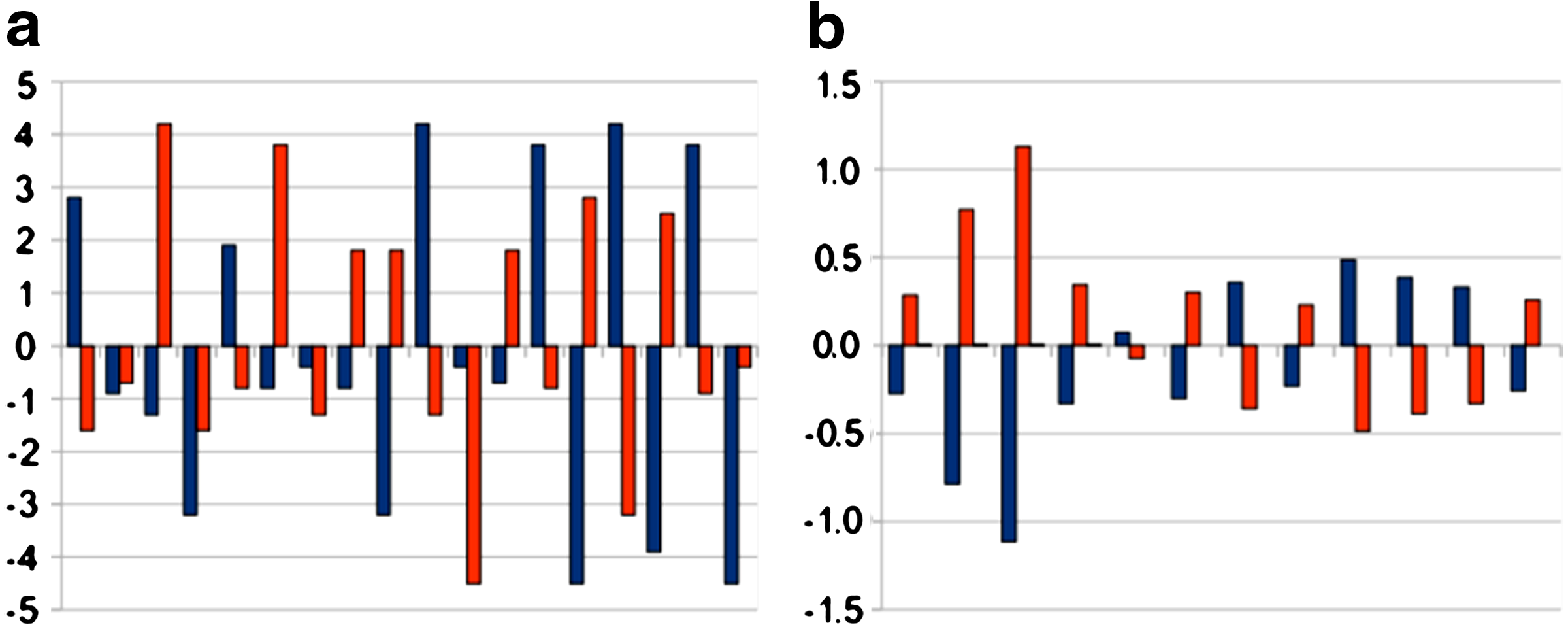
Figure 1a shows the pairwise comparison between the values of the hydropathic coefficients of the amino acids in the Semaphorin-3A sequence and in its complement found by Williams et al. (2005) with a window width W = 7. Figure 1b shows the comparison between the aggregate values on each window for the same two sequences. It is remarkable that in the former case no regularity is observed, whereas in the latter it is clear that for each window the aggregate values of the two sequences are always almost perfectly opposite in sign.

OPEN IN VIEWER

Fig. 1.

Comparison of hydropathic values and profiles between target and complementary peptides. (a) Hydropathic values of target (blue) and complement (red). (b) Hydropathic profiles of target (blue) and complement (red), and their difference (yellow).

3. An Exact Optimization Method

Assume that all possible distinct subsequences of amino acids of length W have been enumerated a priori. We build a graph \documentclass{aastex} \usepackage{amsbsy} \usepackage{amsfonts} \usepackage{amssymb} \usepackage{bm} \usepackage{mathrsfs} \usepackage{pifont} \usepackage{stmaryrd} \usepackage{textcomp} \usepackage{portland, xspace} \usepackage{amsmath, amsxtra} \pagestyle{empty} \DeclareMathSizes {10} {9} {7} {6} \begin{document} $${\cal G}$$\end{document} whose nodes are partitioned into layers that are classes of the partition, one for each \documentclass{aastex} \usepackage{amsbsy} \usepackage{amsfonts} \usepackage{amssymb} \usepackage{bm} \usepackage{mathrsfs} \usepackage{pifont} \usepackage{stmaryrd} \usepackage{textcomp} \usepackage{portland, xspace} \usepackage{amsmath, amsxtra} \pagestyle{empty} \DeclareMathSizes {10} {9} {7} {6} \begin{document} $$w = w_{min} , \ldots , w_{max}$$\end{document} . Each node of \documentclass{aastex} \usepackage{amsbsy} \usepackage{amsfonts} \usepackage{amssymb} \usepackage{bm} \usepackage{mathrsfs} \usepackage{pifont} \usepackage{stmaryrd} \usepackage{textcomp} \usepackage{portland, xspace} \usepackage{amsmath, amsxtra} \pagestyle{empty} \DeclareMathSizes {10} {9} {7} {6} \begin{document} $${\cal G}$$\end{document} in a layer w corresponds to a subsequence of length W in position w; hence, each layer contains as many nodes as the number of distinct subsequences of length W (i.e., \documentclass{aastex} \usepackage{amsbsy} \usepackage{amsfonts} \usepackage{amssymb} \usepackage{bm} \usepackage{mathrsfs} \usepackage{pifont} \usepackage{stmaryrd} \usepackage{textcomp} \usepackage{portland, xspace} \usepackage{amsmath, amsxtra} \pagestyle{empty} \DeclareMathSizes {10} {9} {7} {6} \begin{document} $$\mid {\cal A} \mid ^W$$\end{document} ). The nodes of \documentclass{aastex} \usepackage{amsbsy} \usepackage{amsfonts} \usepackage{amssymb} \usepackage{bm} \usepackage{mathrsfs} \usepackage{pifont} \usepackage{stmaryrd} \usepackage{textcomp} \usepackage{portland, xspace} \usepackage{amsmath, amsxtra} \pagestyle{empty} \DeclareMathSizes {10} {9} {7} {6} \begin{document} $${\cal G}$$\end{document} are weighted: the weight of a node in layer w is the w-th term in the objective function, which depends on the complementarity achieved if a particular subsequence appears in position w. Arcs exist between two nodes of consecutive layers in \documentclass{aastex} \usepackage{amsbsy} \usepackage{amsfonts} \usepackage{amssymb} \usepackage{bm} \usepackage{mathrsfs} \usepackage{pifont} \usepackage{stmaryrd} \usepackage{textcomp} \usepackage{portland, xspace} \usepackage{amsmath, amsxtra} \pagestyle{empty} \DeclareMathSizes {10} {9} {7} {6} \begin{document} $${\cal G}$$\end{document} if and only if the corresponding subsequences are compatible. Two subsequences having nodes in layers w and w + 1 are defined to be compatible if and only if they can appear in consecutive positions in a full sequence, that is if and only if the last W − 1 elements of the subsequence in layer w are the same as the first W − 1 elements in the subsequence in layer w + 1, as illustrated in Figure 2 through an arbitrary example.

OPEN IN VIEWER

Fig. 2.

An arbitrary example of two compatible subsequences of length W = 7.

Graph \documentclass{aastex} \usepackage{amsbsy} \usepackage{amsfonts} \usepackage{amssymb} \usepackage{bm} \usepackage{mathrsfs} \usepackage{pifont} \usepackage{stmaryrd} \usepackage{textcomp} \usepackage{portland, xspace} \usepackage{amsmath, amsxtra} \pagestyle{empty} \DeclareMathSizes {10} {9} {7} {6} \begin{document} $${\cal G}$$\end{document} is directed and acyclic. In principle, computing a shortest path from any node of the first layer to any node of the last layer in \documentclass{aastex} \usepackage{amsbsy} \usepackage{amsfonts} \usepackage{amssymb} \usepackage{bm} \usepackage{mathrsfs} \usepackage{pifont} \usepackage{stmaryrd} \usepackage{textcomp} \usepackage{portland, xspace} \usepackage{amsmath, amsxtra} \pagestyle{empty} \DeclareMathSizes {10} {9} {7} {6} \begin{document} $${\cal G}$$\end{document} yields the optimal solution of the maximum complementarity problem in pseudo-polynomial time. Unfortunately, this construction is impractical because the size of \documentclass{aastex} \usepackage{amsbsy} \usepackage{amsfonts} \usepackage{amssymb} \usepackage{bm} \usepackage{mathrsfs} \usepackage{pifont} \usepackage{stmaryrd} \usepackage{textcomp} \usepackage{portland, xspace} \usepackage{amsmath, amsxtra} \pagestyle{empty} \DeclareMathSizes {10} {9} {7} {6} \begin{document} $${\cal G}$$\end{document} is exponential in W: the number of nodes is \documentclass{aastex} \usepackage{amsbsy} \usepackage{amsfonts} \usepackage{amssymb} \usepackage{bm} \usepackage{mathrsfs} \usepackage{pifont} \usepackage{stmaryrd} \usepackage{textcomp} \usepackage{portland, xspace} \usepackage{amsmath, amsxtra} \pagestyle{empty} \DeclareMathSizes {10} {9} {7} {6} \begin{document} $$( w_{max} - w_{min} + 1 ) \mid {\cal A} \mid ^W$$\end{document} . For instance, for Semaphorin-3A, this number would be equal to 12 × 20⁷ = 15,360,000,000. Even considering that amino acids with the same hydropathic coefficent value are equivalent for our purpose, and noting that amino acids Q, E, N, and D have the same value −3.5, we still have a number of nodes equal to 12 × 17⁷ = 4,924,064,076. If dynamic programming algorithms are used to solve the problem, the construction of \documentclass{aastex} \usepackage{amsbsy} \usepackage{amsfonts} \usepackage{amssymb} \usepackage{bm} \usepackage{mathrsfs} \usepackage{pifont} \usepackage{stmaryrd} \usepackage{textcomp} \usepackage{portland, xspace} \usepackage{amsmath, amsxtra} \pagestyle{empty} \DeclareMathSizes {10} {9} {7} {6} \begin{document} $${\cal G}$$\end{document} can be performed layer by layer incrementally, but even in this case the number of nodes to be handled at the same time can be reduced at most by a small constant factor.

For this reason, we use a different construction: we neglect the order in which the amino acids appear in the subsequences, and we only consider all possible distinct (unordered) multi-sets of cardinality W instead of all possible distinct (ordered) subsequences of length W. In this way, we reduce the size of \documentclass{aastex} \usepackage{amsbsy} \usepackage{amsfonts} \usepackage{amssymb} \usepackage{bm} \usepackage{mathrsfs} \usepackage{pifont} \usepackage{stmaryrd} \usepackage{textcomp} \usepackage{portland, xspace} \usepackage{amsmath, amsxtra} \pagestyle{empty} \DeclareMathSizes {10} {9} {7} {6} \begin{document} $${\cal G}$$\end{document} by a factor which is almost equal to W! (almost, because multi-sets with repeated elements correspond to less than W! distinct subsequences). However, the weights associated with the vertices are the same as before, because all subsequences made of the same elements give the same contribution to the objective function. On the contrary, the definition of compatibility changes: two multi-sets corresponding to nodes in consecutive layers are now defined to be compatible if and only if they share at least W − 1 elements. This relaxed definition of compatibility allows the construction of paths which do not correspond to feasible solutions. An arbitrary example is illustrated in Figure 3.

OPEN IN VIEWER

Fig. 3.

An arbitrary example of compatible multi-sets not corresponding to a feasible solution.

To ensure feasibility while constructing a path along the digraph, it is furthermore necessary to explicitly check that an amino acid entering the multi-set in a given layer leaves the multi-set exactly W iterations later. This is done in a dynamic programming algorithm, based on the following definition of state. A state is a tuple (w, S, f, T, P), where w is the position of the window center in the current sequence, S is a multi-set of amino acids of cardinality W, f is the objective function value, and T is the multi-set of amino acids that can leave the window while moving from position w to position w + 1; finally, the entity P is a sequence pattern representing the sliding window, that is a string of length W containing in each position either an amino acid identifier or a wildcard character ′*′. We indicate as P_j the element in position j of P. If P_j = ′*′, any of the amino acids in T can leave the window during the transition from layer w + j − 1 to layer w + j; otherwise, the amino acid P_j has to be that leaving the window during such transition. That is, the amino acids in T are those which can replace wildcard characters in P. Considering the example in Figure 3 and assuming the first three layers are represented, a state in the second layer would have T = {G, H, M, V, W, Y} and P = ′******S′.

The algorithm starts from a set of initial states, one for each node of the first layer, having the form (w_min, S, C, S, P), where S is each distinct multi-set of cardinality W, C is the corresponding cost, and P is a string of W wildcard characters.

Feasible extensions of states from each layer to the next depend on both T and P. In particular, a state (w, S, f, T, P) can be extended only to nodes of the next layer corresponding to compatible multi-sets S′. Furthermore, if P₁ ≠ ′*′, then the amino acid leaving the window has to be P₁, and so (S\S′) ⊆ {P₁}; on the other hand, if P₁ = ′*′, then the amino acid leaving the window has to be in T, that is (S\S′) ⊆ T.

Provided the extension is feasible, and indicating as C′ the cost corresponding to S′, a new state (w + 1, S′, f ′, P′, T′) is created as follows: \documentclass{aastex} \usepackage{amsbsy} \usepackage{amsfonts} \usepackage{amssymb} \usepackage{bm} \usepackage{mathrsfs} \usepackage{pifont} \usepackage{stmaryrd} \usepackage{textcomp} \usepackage{portland, xspace} \usepackage{amsmath, amsxtra} \pagestyle{empty} \DeclareMathSizes {10} {9} {7} {6} \begin{document} \begin{align*} f^{ \prime} &= f + C^{ \prime} \\ P_j^{ \prime} &= P_{j + 1} \quad \forall j = 1 \ldots W - 1 \\ T^{ \prime} &= T \setminus ( S \setminus S^{ \prime} ) \\ P^{ \prime}_{ W } &= \begin{cases}{\rm unique} \ { \rm element} \ { \rm of} \ S^{ \prime} \setminus S \quad{\rm if} \ S^{ \prime} \setminus S \neq\, \emptyset \\ P_1 \quad\quad\quad\quad\quad\quad\quad\quad\quad\quad{\rm otherwise}\end{cases}\end{align*}\end{document}

that is, beside increasing the partial cost, if S ≠ S′ we delete from T the unique element in S\S′, we delete from P its first element and append to P the unique element in S′\S. Instead, if S = S′, either P₁ ≠ ′*′ and then the amino acid \documentclass{aastex} \usepackage{amsbsy} \usepackage{amsfonts} \usepackage{amssymb} \usepackage{bm} \usepackage{mathrsfs} \usepackage{pifont} \usepackage{stmaryrd} \usepackage{textcomp} \usepackage{portland, xspace} \usepackage{amsmath, amsxtra} \pagestyle{empty} \DeclareMathSizes {10} {9} {7} {6} \begin{document} $$P_{W}^{\prime}$$\end{document} entering the window has to be the same as that leaving the window, or P₁ = ′*′ and then the amino acid entering the window can be any of those in T, and therefore \documentclass{aastex} \usepackage{amsbsy} \usepackage{amsfonts} \usepackage{amssymb} \usepackage{bm} \usepackage{mathrsfs} \usepackage{pifont} \usepackage{stmaryrd} \usepackage{textcomp} \usepackage{portland, xspace} \usepackage{amsmath, amsxtra} \pagestyle{empty} \DeclareMathSizes {10} {9} {7} {6} \begin{document} $$P_{W}^{\prime}$$\end{document} has still to be marked with ′*′; in both cases, \documentclass{aastex} \usepackage{amsbsy} \usepackage{amsfonts} \usepackage{amssymb} \usepackage{bm} \usepackage{mathrsfs} \usepackage{pifont} \usepackage{stmaryrd} \usepackage{textcomp} \usepackage{portland, xspace} \usepackage{amsmath, amsxtra} \pagestyle{empty} \DeclareMathSizes {10} {9} {7} {6} \begin{document} $$P_{W}^{\prime} = P_1$$\end{document} .

Final states are those of layer w_max, and the minimum cost state among them corresponds to an optimal solution.

The dominance criterion used to fathom useless states is the following: (w′, S′, f ′, T ′, P′) dominates (w″, S″, f ″, T ″, P″) only if \documentclass{aastex} \usepackage{amsbsy} \usepackage{amsfonts} \usepackage{amssymb} \usepackage{bm} \usepackage{mathrsfs} \usepackage{pifont} \usepackage{stmaryrd} \usepackage{textcomp} \usepackage{portland, xspace} \usepackage{amsmath, amsxtra} \pagestyle{empty} \DeclareMathSizes {10} {9} {7} {6} \begin{document} \begin{align*} & w^{ \prime \prime} = w^{ \prime} \\ & f^{ \prime \prime} \geq \,f^{ \prime} \\ & T^{ \prime \prime} \subseteq T^{ \prime} \\ & P^{ \prime \prime} = P^{ \prime}\end{align*}\end{document}

Given any upper bound U on the overall value of the objective function, we can discard all multi-sets for which the sum of the hydropathic coefficients is too far from 0 to be balanced by a complementary multi-set (this is checked during the initial enumeration) as well as all dynamic programming states with \documentclass{aastex} \usepackage{amsbsy} \usepackage{amsfonts} \usepackage{amssymb} \usepackage{bm} \usepackage{mathrsfs} \usepackage{pifont} \usepackage{stmaryrd} \usepackage{textcomp} \usepackage{portland, xspace} \usepackage{amsmath, amsxtra} \pagestyle{empty} \DeclareMathSizes {10} {9} {7} {6} \begin{document} $$f > \sqrt{U}$$\end{document} (this is checked in the dynamic programming algorithm).

To apply these two fathoming techniques, we need good upper bounds that can be easily provided by heuristics.

The complete algorithm is divided into three steps. Step 1 consists of the computation of an upper bound U with any heuristic technique. In Step 2, the digraph \documentclass{aastex} \usepackage{amsbsy} \usepackage{amsfonts} \usepackage{amssymb} \usepackage{bm} \usepackage{mathrsfs} \usepackage{pifont} \usepackage{stmaryrd} \usepackage{textcomp} \usepackage{portland, xspace} \usepackage{amsmath, amsxtra} \pagestyle{empty} \DeclareMathSizes {10} {9} {7} {6} \begin{document} $${\cal G}$$\end{document} is constructed: for each position w of the sliding window, the algorithm enumerates all multi-sets of cardinality W and discards those whose overall weight (the sum of the hydropathic coefficients of the W amino acids) is too different (more than \documentclass{aastex} \usepackage{amsbsy} \usepackage{amsfonts} \usepackage{amssymb} \usepackage{bm} \usepackage{mathrsfs} \usepackage{pifont} \usepackage{stmaryrd} \usepackage{textcomp} \usepackage{portland, xspace} \usepackage{amsmath, amsxtra} \pagestyle{empty} \DeclareMathSizes {10} {9} {7} {6} \begin{document} $$\sqrt{U}$$\end{document} ) from the target value −C(w). For each enumerated multi-set, a weighted node is inserted into layer w of digraph \documentclass{aastex} \usepackage{amsbsy} \usepackage{amsfonts} \usepackage{amssymb} \usepackage{bm} \usepackage{mathrsfs} \usepackage{pifont} \usepackage{stmaryrd} \usepackage{textcomp} \usepackage{portland, xspace} \usepackage{amsmath, amsxtra} \pagestyle{empty} \DeclareMathSizes {10} {9} {7} {6} \begin{document} $${\cal G}$$\end{document} . Finally, Step 3A consists of the dynamic programming algorithm described above, to compute the shortest path on \documentclass{aastex} \usepackage{amsbsy} \usepackage{amsfonts} \usepackage{amssymb} \usepackage{bm} \usepackage{mathrsfs} \usepackage{pifont} \usepackage{stmaryrd} \usepackage{textcomp} \usepackage{portland, xspace} \usepackage{amsmath, amsxtra} \pagestyle{empty} \DeclareMathSizes {10} {9} {7} {6} \begin{document} $${\cal G}$$\end{document} . The last step can be replaced by a Step 3B in which the dynamic programming algorithm is run without the dominance test. In this way, all paths with cost not greater than UB are found.

We remark that Step 2 does not require the explicit enumeration of all multi-sets of cardinality W, especially if the upper bound U is close to 0. We also remark that Step 3A or 3B can be easily implemented as a label setting algorithm because \documentclass{aastex} \usepackage{amsbsy} \usepackage{amsfonts} \usepackage{amssymb} \usepackage{bm} \usepackage{mathrsfs} \usepackage{pifont} \usepackage{stmaryrd} \usepackage{textcomp} \usepackage{portland, xspace} \usepackage{amsmath, amsxtra} \pagestyle{empty} \DeclareMathSizes {10} {9} {7} {6} \begin{document} $${\cal G}$$\end{document} is acyclic.

4. Experimental Results

In this section, we compare the performance of our algorithm to that of existing methods from the literature. We take into account two aspects of our algorithm: the computational behavior and the quality of the peptides produced. In our experiments, we set the hydropathic coefficient c_i of each amino acid \documentclass{aastex} \usepackage{amsbsy} \usepackage{amsfonts} \usepackage{amssymb} \usepackage{bm} \usepackage{mathrsfs} \usepackage{pifont} \usepackage{stmaryrd} \usepackage{textcomp} \usepackage{portland, xspace} \usepackage{amsmath, amsxtra} \pagestyle{empty} \DeclareMathSizes {10} {9} {7} {6} \begin{document} $$i \in {\cal A}$$\end{document} according to the Kyte and Doolittle scale, although many others were presented and compared in the literature (Jääskeläinen et al., 2007). This was done to compare with previous approaches, as the same scale has been used by both Williams et al. (2005) and Fassina and Cassani (1992).

4.2. Experiments on human interleukin 1β

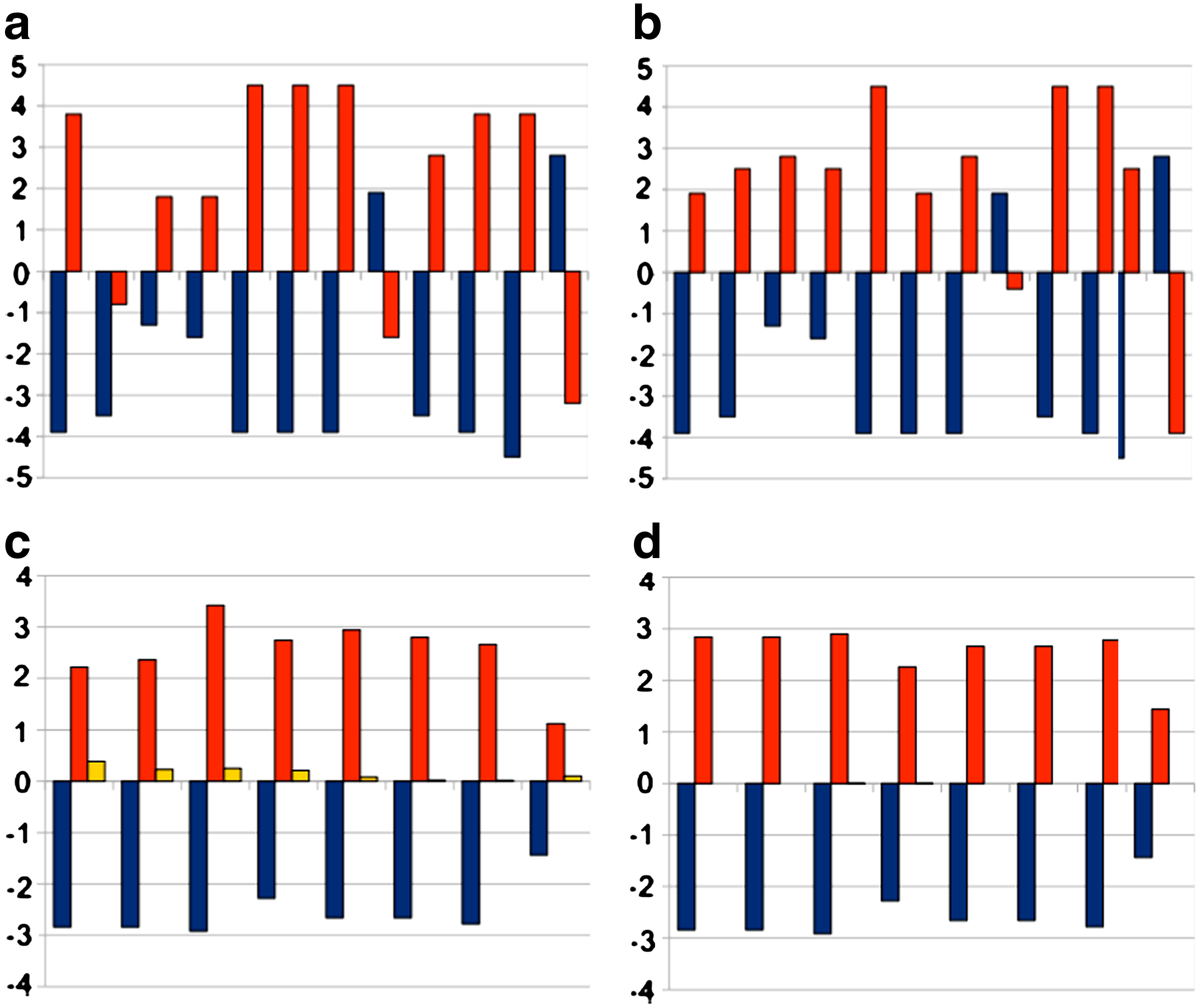
In a second set of experiments, we considered as a target the human interleukin 1β (KNYPKKKMEKRF). In this way, we could compare to Fassina and Cassani (1992), where complementary peptides were identified using the heuristic approach implemented in the AMINOMAT software tool. The best sequence found by AMINOMAT (indicated as AM in the remainder) is HLLFPIIIAASL with an HC score of 0.401746, and was found by the authors by optimizing with respect to the HC criterion only; our algorithm, instead, was able to solve the problem to proven optimality in 0.10 seconds, and identified the sequence KCIIGFMICFCM (indicated as opt in the remainder) as an optimal one, having an HC score of 0.01. In Figure 4a, b, we compare hydropathic values of amino acids in corresponding positions respectively in the target-AM pair and target-opt pair; in Figure 4c, d, the average hydropathic score in each sliding window, in respectively, the target-AM pair and the target-opt pair is represented (in all figures, the red bars represent the final score in each sliding window). As discussed in Section 2, it is interesting to note that a better average hydropathic score is obtained by allowing less regularity in the complementary sequence.

OPEN IN VIEWER

Fig. 4.

Comparison of hydropathic values and profiles between target, AM and opt peptides on human interleukin 1β. (a) Hydropathic values of target (blue) and AM (red) peptides. (b) Hydropathic values of target (blue) and opt (red) peptides. (c) Hydropathic profiles of target (blue) and AM (red) peptides, and their difference (yellow). (d) Hydropathic profiles of target (blue) and opt (red) peptides, and their difference (yellow).

5. Conclusion

In this article, we tried to tackle a problem arising in drug design using combinatorial optimization techniques. We designed an effective algorithm and built a computing tool that can find a proven global optimum in a few seconds on a notebook computer. With our method, we could also enumerate and score a number of good solutions in an additional short computing time. The source code of a prototype C++ implementation of our algorithms is freely available for noncommercial use on the web (Ceselli et al., 2010).

As a main result, we showed that in this context mathematical programming methods are more successful than heuristics such as simulated annealing. In fact, our exact method can provide in a few seconds solutions with a global optimality guarantee. As a side effect, we also proved the optimality of the solution given by Williams et al. (2005) for the Semaphorin-3A, and we found a solution with a better score than that given by AMINOMAT for the human interleukin 1β.

We also used our tool to evaluate different solutions according to both HC and AH scoring methods. From our analysis, HC and AH appear as different criteria, not always consistent, for scoring peptides. The AH score seems particularly difficult to compute in an effective way, since the antisense complement of each amino acid can be defined with some degree of freedom (Heal et al., 2002); also the computation of the HC score allows some degree of freedom, as many hydropathy scales have been proposed in the literature (Jääskeläinen et al., 2007). In this setting, our algorithm unfolds its potential, being able to provide not only a single optimal solution, but a ranking of provable good ones; this ranking can then be used by biologists as a starting basis for further refinements, simulations, or in vitro experiments.

In the future, we aim to upgrade our method in order to enumerate all the Pareto-optimal solutions with respect to HC, AH, and other criteria; in fact, the same methodology can be applied to other scoring functions already successfully tested in different contexts (Pandini et al., 2010). This could yield a useful tool for evalutating the effectiveness of MRT-like techniques for identifying complementary peptides of different molecules.

To validate the rankings produced by different criteria, we are also experimenting on combining optimization techniques with molecular dynamics simulations.

References

1.
BaranyiL., CampbellW., OhshimaK.et al.1995. The antisense homology box: a new motif within proteins that encodes biologically active peptides. Nat. Med., 1:894–901.
2.
BlalockJ.1995. Genetic origins of protein shape and interaction rules. Nat. Med., 1:876–878.
DayhoffM., SchwartzR., OrcuttB.1978. A model of evolutionary change in proteins. Atlas Protein Seq. Struct., 5:345–352.
5.
FassinaG., CassaniG.1992. Design and recognition properties of a hydropathically complementary peptide to human interleukin 1βBiochem. J., 282:773–779.
6.
GareyM., JohnsonD.1979. Computers and Intractability: A Guide to the Theory of NP-Completeness. W.H. Freeman: New York.
7.
HealJ., RobertsG., RaynesJ.et al.2002. Specific interactions between sense and complementary peptides: the basis for the proteomic code. Chem. Biol. Chem., 3:136–151.
8.
JääskeläinenS., RiikonenP., SalakoskiT.et al.2007. Evaluation of protein hydropathy scales. Proc. IEEE Int. Conf. Bioinform. Biomed., 245–251.
9.
KyteJ., DoolittleR.1982. A simple method for displaying the hydropathic character of a protein. J. Mol. Biol., 157:105–132.
10.
PandiniA., ForniliA., KleinjungJ.2010. Structural alphabets derived from attractors in conformational space. BMC Bioinform., 11.
11.
SahniS.1974. Computationally related problems. SIAM J. Comput., 3:262–279.
12.
WeathingtonN., van HouwelingenA., NoeragerB.et al.2006. A novel peptide CXCR ligand derived from extracellular matrix degradation during airway inflammation. Nat. Med., 12:317–323.
13.
WilliamsG., EickholtB., MaisonP.et al.2005. A complementary peptide approach applied to the design of novel semaphorin/neuropilin antagonists. J. Neurochem., 92:1180–1190.