Theory and Practice of Ultra-Perfection

Abstract

Perfection has been used as a criteria to classify rearrangement scenarios since 2004. However, there is a fundamental bias towards extant species in the original definition: ancestral species are not bound to perfection. Here we develop a new theory of perfection that takes an egalitarian view of species, and we examine the fitness of this theory on several datasets. Supplementary Material is available at www.liebertonline.com/cmb.

1. Introduction

In mathematical biology, the genome sorting problem is to find a sequence of rearrangement operations that transforms one genome into another. The type of rearrangement operations is fixed, and a sorting sequence of operations is called a scenario. Given two genomes, there can be an exponential number of scenarios, which makes difficult the choice of one particular scenario, even among those of minimum length called parsimonious. Parsimony is only one of the criteria that can be used for the selection of a scenario, and there are many alternatives that are worth exploring.

Here we consider the problem of perfect sorting which was initially stated roughly as follows: given two genomes, find a sorting scenario between the genomes that preserves common genomic segments in intermediate states of the transformation. Such scenarios are called perfect and this problem was first introduced under the inversion rearrangement model by Figeac and Varré (2004) who showed the NP-hardness of the problem. It was later shown by Bérard et al. (2004, 2007), Braga et al. (2009), and Sagot and Tannier (2005) that for some classes of instances, the problem could be solved in polynomial time. More recently, Bérard et al. (2008) explored the problem under the double-cut-and-join (DCJ) rearrangement model, using a less stringent definition of perfection that allows temporary circular chromosomes.

In this article, we address the problem of perfect sorting by DCJ under the initial definition of perfection. We also reexamine the original idea of perfection which applies only to the two compared extant species. What about all intermediate species that are generated by the scenario? Any good biological argument in favor of perfect scenarios would apply to any pair of these intermediate species. In this paper, we intend to correct this injustice. Note that, in Braga et al. (2009), an asymmetric approach that consists in progressively detecting and preserving common segments between intermediate species and one of the extant species was proposed. Here, we present a symmetric approach that considers common segments between all pairs of species.

We introduce a new, more restrictive class of perfection, called ultra-perfection with the corresponding problem: given two genomes, find a sorting scenario such that any sub-scenario is perfect. Our main results are the description of combinatorial properties of ultra-perfection that leads to a polynomial time algorithm for computing ultra-perfect scenarios between genomes, and the discussion of its practicability through real datasets.

This article is organized as follows: in Section 2, we give the definitions of genomes, common intervals, rearrangement scenarios and ultra-perfection. In Section 3, we characterize ultra-perfection in terms of commutation of inversion scenarios, which leads to an algorithm for computing ultra-perfect scenarios. In Section 4, we describe several examples of rearrangement scenarios, on real datasets, ranging from a scenario that breaks almost all common intervals to ultra-perfect scenarios.

2. Models and Definitions

In this section, we give the main definitions and notation that are used in the paper: genomes, inversions, double-cut-and-join operations, commuting inversions, perfect and ultra-perfect scenarios.

2.1. Genomes

Genomes are compared by identifying homologous segments along their DNA sequences, called blocks, organized in circular or linear chromosomes. A genome is circular (resp. linear) if it is only composed of circular (resp. linear) chromosomes. Each genome contains exactly one occurrence of each block, and the order and orientation of the blocks may differ between genomes. A linear chromosome will be represented by an ordered sequence of signed integers, one for each block, flanked by the unsigned block ∘ at each end, and a circular chromosome will be represented by a circularly ordered sequence of signed integers. For example, genome (−5 7 1 −3 2) (∘ −6 4 8 9 ∘) consists of one circular chromosome and one linear chromosome.

An adjacency in a genome is a pair of consecutive blocks. Since a chromosome can be read in two directions; the adjacencies (x y) and (−y − x) are equivalent. Moreover, since the block ∘ is unsigned, the adjacencies (∘ y) and (−y ∘) are equivalent. An interval in a genome is a set of blocks that appear consecutively in the genome. For example, in genome (−5 7 1 − 3 2) (∘ −6 4 8 9 ∘), {−3 2 − 5} and {−6 4} are two intervals. A common interval between genomes A and B is an interval that exists in both A and B. A maximal common interval between A and B is a common interval that is not included in any other common interval between A and B.

2.2. Rearrangement scenarios

In this paper, we consider two models of rearrangements: the inversion model and the double-cut-and-join model. An inversion of a set of contiguous blocks reverses the order of those blocks and change their signs. A double-cut-and-join (DCJ) operation on a genome A cuts two different adjacencies in A and glues pairs of the four exposed extremities to form two new adjacencies, no other adjacency is altered. The circularization of a linear chromosome \documentclass{aastex}\usepackage{amsbsy}\usepackage{amsfonts}\usepackage{amssymb}\usepackage{bm}\usepackage{mathrsfs}\usepackage{pifont}\usepackage{stmaryrd}\usepackage{textcomp}\usepackage{portland, xspace}\usepackage{amsmath, amsxtra}\pagestyle{empty}\DeclareMathSizes{10}{9}{7}{6}\begin{document}$$(\circ x \ldots y \circ)$$\end{document} is the DCJ operation that cuts adjacencies (∘ x) and (y ∘) to produce (y x) and (∘ ∘), thus creating the circular chromosome \documentclass{aastex}\usepackage{amsbsy}\usepackage{amsfonts}\usepackage{amssymb}\usepackage{bm}\usepackage{mathrsfs}\usepackage{pifont}\usepackage{stmaryrd}\usepackage{textcomp}\usepackage{portland, xspace}\usepackage{amsmath, amsxtra}\pagestyle{empty}\DeclareMathSizes{10}{9}{7}{6}\begin{document}$$(x \ldots y)$$\end{document} . The opposite operation called a linearization is a DCJ operation that transforms a circular chromosome into a linear chromosome.

For example, a DCJ operation on genome (−5 7 1 −3 2) (∘ −6 4 8 9 ∘) that cuts the adjacencies (2 − 5) and (−6 4) to form (2 4) and (−6 − 5) would produce genome (∘ −6 −5 7 1 −3 2 4 8 9 ∘). Note that we consider the empty chromosome (∘ ∘) to belong to any genome so that the DCJ on the circular genome (−5 7 1 −3 2) which cuts adjacencies (7 1) and (∘ ∘) will produce the linear genome (∘1 −3 2 −5 7∘).

Let A and B be two genomes. A scenario from A to B is a sequence of rearrangements that transforms A into B. An inversion scenario from A to B contains only inversions, and DCJ scenario contains only DCJ operations. Since an inversion can always be realized by one DCJ operation, an inversion scenario is always a DCJ scenario.

Note that the application of an inversion on a given genome only affects a single chromosome of the genome. Thus, an inversion scenario on a genome A can always be decomposed into a set of independent inversion scenarios, each acting on a single chromosome of genome A. In the following, we will restrict our study of inversion scenarios to unichromosomal genomes.

2.3. Perfection and commutation

The following definition of perfection is used in Bérard et al. (2004, 2007), Figeac and Varré (2004), and Sagot and Tannier (2005):

Definition 1 (Perfection)

A rearrangement scenario from genome A to genome B is perfect if all common intervals of A and B are also intervals in the intermediate genomes of the scenario.

In this paper we introduce a new, more restrictive class of perfection that we call ultra-perfection.

Definition 2 (Ultra-Perfection)

A rearrangement scenario from genome A to genome B is ultra-perfect if all sub-scenarios are perfect.

The difference between the two notions is illustrated by the following example. Consider the two genomes (∘ −3 −1 4 2 ∘) and (∘ 1 2 3 4 ∘) that have no common intervals, except trivial ones. Definition 1 implies that any inversion scenario between the two genomes is perfect. However, as we will show in Section 3, none of these scenarios is ultra-perfect. In particular, the scenario depicted in Figure 1 creates the common interval {2, 3, 4} between chromosomes C₂ and C₄, but destroys it in C₃.

FIG. 1.

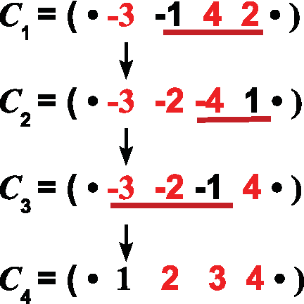
An inversion scenario that sorts (∘ −3 −1 4 2 ∘) into (∘ 1 2 3 4 ∘).

General ultra-perfect DCJ scenarios can break and rearrange chromosomes. For example, genome (∘ 1 2 3 4 ∘) (∘ 5 6 7 8 ∘) can be transformed into genome (∘ 1 2 7 8 ∘)(∘ 5 6 3 4 ∘) with one DCJ operation, and a subsequent scenario may remain ultra-perfect as long as intervals {1, 2, 3, 4} and {5, 6, 7, 8} are not re-created.

As we will see, the notion of ultra-perfection is intimately related with commutation of inversions. We first recall the definition of commutation used in Bérard et al. (2004): two sets of blocks commute if they are either disjoint or one is included in the other. Two inversions commute if their associated sets of blocks commute. For example, in the scenario depicted in Figure 1 the first and the second inversions commute, while the second inversion and the third do not commute. An inversion scenario is commuting if all pairs of inversions contained in the scenario commute.

When considering circular chromosome, the definition of commutation must be adapted. Indeed, in a circular chromosome containing the set of blocks G, an inversion associated to a set S ⊂ G produces the same result as an inversion associated to the set G\S. We thus introduce the circularly commuting property defined as: given a set G of blocks, two subsets S and T of G commute circularly if S and T commute, or G \ S and T commute. For example, in Figure 1, the second inversion and the third inversion do not commute, but they commute circularly.

Note that in Bérard et al. (2008) a less stringent definition of perfection is used for DCJ scenarios. In this version, the notion of common interval is relaxed to allow subsets of common intervals that form circular chromosomes.

3. Ultra-perfect scenarios

We now consider the problem of computing an ultra-perfect scenario between two genomes. In Section 3.1, we show that each maximal common interval can be considered independently. This implies an ultra-perfect scenario that first sorts each substring associated with a maximal common interval, and then sorts the whole genome in its final configuration. Section 3.2 then describes conditions for the existence of ultra-perfect DCJ scenarios between substrings associated to each maximal common interval.

Throughout the section we refer to a substring of a genome associated with an interval as a segment of the genome. The segment of a genome A induced by an interval I is denoted A_I.

3.1. Independent DCJ sorting of maximal common intervals

The following proposition states that, in any ultra-perfect DCJ scenario between genomes A and B, the segments induced by maximal common intervals of A and B are sorted independently.

Proposition 1

Let I be a maximal common interval between genomes A and B. If \documentclass{aastex}\usepackage{amsbsy}\usepackage{amsfonts}\usepackage{amssymb}\usepackage{bm}\usepackage{mathrsfs}\usepackage{pifont}\usepackage{stmaryrd}\usepackage{textcomp}\usepackage{portland, xspace}\usepackage{amsmath, amsxtra}\pagestyle{empty}\DeclareMathSizes{10}{9}{7}{6}\begin{document}$${\cal S}$$\end{document} is an ultra-perfect DCJ scenario from A to B, then there exists an equal length ultra-perfect scenario \documentclass{aastex}\usepackage{amsbsy}\usepackage{amsfonts}\usepackage{amssymb}\usepackage{bm}\usepackage{mathrsfs}\usepackage{pifont}\usepackage{stmaryrd}\usepackage{textcomp}\usepackage{portland, xspace}\usepackage{amsmath, amsxtra}\pagestyle{empty}\DeclareMathSizes{10}{9}{7}{6}\begin{document}$${\cal S}^{\prime} = {\cal S}_I {\cal T}$$\end{document} such that \documentclass{aastex}\usepackage{amsbsy}\usepackage{amsfonts}\usepackage{amssymb}\usepackage{bm}\usepackage{mathrsfs}\usepackage{pifont}\usepackage{stmaryrd}\usepackage{textcomp}\usepackage{portland, xspace}\usepackage{amsmath, amsxtra}\pagestyle{empty}\DeclareMathSizes{10}{9}{7}{6}\begin{document}$${\cal S}_I$$\end{document} is an ultra-perfect DCJ scenario transforming A_I into B_I.

Proof

Let C be a genome obtained by applying some (possibly empty) prefix of \documentclass{aastex}\usepackage{amsbsy}\usepackage{amsfonts}\usepackage{amssymb}\usepackage{bm}\usepackage{mathrsfs}\usepackage{pifont}\usepackage{stmaryrd}\usepackage{textcomp}\usepackage{portland, xspace}\usepackage{amsmath, amsxtra}\pagestyle{empty}\DeclareMathSizes{10}{9}{7}{6}\begin{document}$${\cal S}$$\end{document} , and D be the genome obtained by applying some subsequent operations of \documentclass{aastex}\usepackage{amsbsy}\usepackage{amsfonts}\usepackage{amssymb}\usepackage{bm}\usepackage{mathrsfs}\usepackage{pifont}\usepackage{stmaryrd}\usepackage{textcomp}\usepackage{portland, xspace}\usepackage{amsmath, amsxtra}\pagestyle{empty}\DeclareMathSizes{10}{9}{7}{6}\begin{document}$${\cal S}$$\end{document} on C. Since \documentclass{aastex}\usepackage{amsbsy}\usepackage{amsfonts}\usepackage{amssymb}\usepackage{bm}\usepackage{mathrsfs}\usepackage{pifont}\usepackage{stmaryrd}\usepackage{textcomp}\usepackage{portland, xspace}\usepackage{amsmath, amsxtra}\pagestyle{empty}\DeclareMathSizes{10}{9}{7}{6}\begin{document}$${\cal S}$$\end{document} is ultra-perfect, I is an interval of C and D. Say that the operation transforming the intermediate genome C into the intermediate genome D modifies I if C_I ≠ D_I.

Let f be an operation of \documentclass{aastex}\usepackage{amsbsy}\usepackage{amsfonts}\usepackage{amssymb}\usepackage{bm}\usepackage{mathrsfs}\usepackage{pifont}\usepackage{stmaryrd}\usepackage{textcomp}\usepackage{portland, xspace}\usepackage{amsmath, amsxtra}\pagestyle{empty}\DeclareMathSizes{10}{9}{7}{6}\begin{document}$${\cal S}$$\end{document} such that f modifies I and the operation e preceding f does not modify I. If f cuts no adjacency created by e, then simply switch the order of e and f. Otherwise we replace e and f by two DCJs e′ and f′ such that e′ precedes f′, through the following process: say e cuts the adjacency (u v) and (y x), u being a block belonging to I, to create (u x) and (y v), and that f then cuts (u x) and (t s) to create (u s) and (t x). Then take DCJs e′ and f′ such that e′ cuts the adjacency (u v) and (t s) to create (u s) and (t v), and f′ cuts (t v) and (y x) to create (t x) and (y v). In this way, any operations modifying I can be moved to the beginning of the DCJ scenario. Each move does not effect the ultra-perfection of the scenario since e′ cannot create an interval that is later broken: any new interval created by e′ (and later broken by some DCJ g) would have to include some elements of I and some adjacent elements to I. But this implies the existence of a larger interval that would be broken by g in the original scenario.

Moreover, at the end of this process, the scenario obtained can be decomposed into two sequences \documentclass{aastex}\usepackage{amsbsy}\usepackage{amsfonts}\usepackage{amssymb}\usepackage{bm}\usepackage{mathrsfs}\usepackage{pifont}\usepackage{stmaryrd}\usepackage{textcomp}\usepackage{portland, xspace}\usepackage{amsmath, amsxtra}\pagestyle{empty}\DeclareMathSizes{10}{9}{7}{6}\begin{document}$${\cal S}_I$$\end{document} and \documentclass{aastex}\usepackage{amsbsy}\usepackage{amsfonts}\usepackage{amssymb}\usepackage{bm}\usepackage{mathrsfs}\usepackage{pifont}\usepackage{stmaryrd}\usepackage{textcomp}\usepackage{portland, xspace}\usepackage{amsmath, amsxtra}\pagestyle{empty}\DeclareMathSizes{10}{9}{7}{6}\begin{document}$${\cal T}$$\end{document} such that all operations in \documentclass{aastex}\usepackage{amsbsy}\usepackage{amsfonts}\usepackage{amssymb}\usepackage{bm}\usepackage{mathrsfs}\usepackage{pifont}\usepackage{stmaryrd}\usepackage{textcomp}\usepackage{portland, xspace}\usepackage{amsmath, amsxtra}\pagestyle{empty}\DeclareMathSizes{10}{9}{7}{6}\begin{document}$${\cal S}_I$$\end{document} modify I but no operation in \documentclass{aastex}\usepackage{amsbsy}\usepackage{amsfonts}\usepackage{amssymb}\usepackage{bm}\usepackage{mathrsfs}\usepackage{pifont}\usepackage{stmaryrd}\usepackage{textcomp}\usepackage{portland, xspace}\usepackage{amsmath, amsxtra}\pagestyle{empty}\DeclareMathSizes{10}{9}{7}{6}\begin{document}$${\cal T}$$\end{document} modifies I. Then, \documentclass{aastex}\usepackage{amsbsy}\usepackage{amsfonts}\usepackage{amssymb}\usepackage{bm}\usepackage{mathrsfs}\usepackage{pifont}\usepackage{stmaryrd}\usepackage{textcomp}\usepackage{portland, xspace}\usepackage{amsmath, amsxtra}\pagestyle{empty}\DeclareMathSizes{10}{9}{7}{6}\begin{document}$${\cal S}_I$$\end{document} is an ultra-perfect DCJ scenario between the segments A_I and B_I. ▪

3.2. Ultra-perfect scenarios between unichromosomal genomes

Proposition 1 implies that, for each maximal common interval I of A and B, the ultra-perfect sorting of A_I into B_I can be examined independently from the rest of the scenario. We now give characterizations of the existence of ultra-perfect DCJ scenarios between unichromosomal genomes A and B by establishing properties of commuting inversion scenarios.

Ultra-perfect inversion scenarios

First, we characterize ultra-perfect inversion scenarios.

Proposition 2

An inversion scenario between two linear genomes is ultra-perfect if and only if the scenario is commuting.

Proof

Bérard et al. (2007) shows that a commuting inversion scenario is always perfect. So, if a scenario \documentclass{aastex}\usepackage{amsbsy}\usepackage{amsfonts}\usepackage{amssymb}\usepackage{bm}\usepackage{mathrsfs}\usepackage{pifont}\usepackage{stmaryrd}\usepackage{textcomp}\usepackage{portland, xspace}\usepackage{amsmath, amsxtra}\pagestyle{empty}\DeclareMathSizes{10}{9}{7}{6}\begin{document}$${\cal S}$$\end{document} is commuting, then all sub-scenarios of \documentclass{aastex}\usepackage{amsbsy}\usepackage{amsfonts}\usepackage{amssymb}\usepackage{bm}\usepackage{mathrsfs}\usepackage{pifont}\usepackage{stmaryrd}\usepackage{textcomp}\usepackage{portland, xspace}\usepackage{amsmath, amsxtra}\pagestyle{empty}\DeclareMathSizes{10}{9}{7}{6}\begin{document}$${\cal S}$$\end{document} are commuting and thus perfect. Commutation then implies ultra-perfection.

Next, let \documentclass{aastex}\usepackage{amsbsy}\usepackage{amsfonts}\usepackage{amssymb}\usepackage{bm}\usepackage{mathrsfs}\usepackage{pifont}\usepackage{stmaryrd}\usepackage{textcomp}\usepackage{portland, xspace}\usepackage{amsmath, amsxtra}\pagestyle{empty}\DeclareMathSizes{10}{9}{7}{6}\begin{document}$${\cal S}$$\end{document} be an ultra-perfect scenario. Suppose that \documentclass{aastex}\usepackage{amsbsy}\usepackage{amsfonts}\usepackage{amssymb}\usepackage{bm}\usepackage{mathrsfs}\usepackage{pifont}\usepackage{stmaryrd}\usepackage{textcomp}\usepackage{portland, xspace}\usepackage{amsmath, amsxtra}\pagestyle{empty}\DeclareMathSizes{10}{9}{7}{6}\begin{document}$${\cal S}$$\end{document} is not commuting. Then there exists two inversions in \documentclass{aastex}\usepackage{amsbsy}\usepackage{amsfonts}\usepackage{amssymb}\usepackage{bm}\usepackage{mathrsfs}\usepackage{pifont}\usepackage{stmaryrd}\usepackage{textcomp}\usepackage{portland, xspace}\usepackage{amsmath, amsxtra}\pagestyle{empty}\DeclareMathSizes{10}{9}{7}{6}\begin{document}$${\cal S}$$\end{document} , e preceding f, such that e and f do not commute but e and f commute with all inversions in \documentclass{aastex}\usepackage{amsbsy}\usepackage{amsfonts}\usepackage{amssymb}\usepackage{bm}\usepackage{mathrsfs}\usepackage{pifont}\usepackage{stmaryrd}\usepackage{textcomp}\usepackage{portland, xspace}\usepackage{amsmath, amsxtra}\pagestyle{empty}\DeclareMathSizes{10}{9}{7}{6}\begin{document}$${\cal S}$$\end{document} between e and f.

Say, without loss of generality, that the genome looks like UVWXY before applying inversion e where U, V, W, X, and Y represent sets of blocks. In this configuration e = {V, W} and f = {V, X}, and all inversions in the scenario between e and f, then, do not change the relative order of V, W, and X to each other (since they commute with e and f). So e creates the order WVX while f creates the order WXV. But this contradicts the hypothesis that \documentclass{aastex}\usepackage{amsbsy}\usepackage{amsfonts}\usepackage{amssymb}\usepackage{bm}\usepackage{mathrsfs}\usepackage{pifont}\usepackage{stmaryrd}\usepackage{textcomp}\usepackage{portland, xspace}\usepackage{amsmath, amsxtra}\pagestyle{empty}\DeclareMathSizes{10}{9}{7}{6}\begin{document}$${\cal S}$$\end{document} is ultra-perfect since the interval {W, X} is destroyed by e and recreated by f. ▪

In Bérard et al. (2007), it was shown that the commuting inversion scenarios between linear genomes could be characterized in terms of the structure of a tree, called the strong interval tree, representing the set of all common intervals. The strong interval tree of two linear genomes is a tree whose vertices are the common intervals that commute with any other common interval and there is an edge (I, J) between two vertices if J ⊂ I and there exist no third vertex K such that J ⊂ K ⊂ I. The strong interval tree was first described in Heber and Stoye (2001), Landau et al. (2005), and Bergeron et al. (2005), and it was inspired from a data structure called the PQ-tree. PQ-trees are used to represent all consecutive-ones orderings of the columns of a matrix that has the consecutive-ones property.

In the remainder of the section, we develop the counterpart characterization for DCJ scenarios by relating ultra-perfect DCJ scenarios to a tree representing the set of all common intervals between two circular genomes. We present the circular common interval tree that is the circular analogue of the strong interval tree. Circular common interval trees are inspired from an analogous structure of a PQ-tree, called a PC-tree. The PC-tree was introduced in Hsu (2001) and Hsu and McConnell (2003), where it was used to represent all circular-ones orderings of the columns of a matrix that has the circular-ones property.

Circular common interval tree

Here, we define a tree representing the set of all common intervals between two circular genomes. Let G be a set of n blocks, and A and B be two circular genomes on G. A circular common interval of A and B is either a singleton block, or a subset I of G such that I is a common interval between A and B, and |I| ≠ n − 1. The circular strong intervals of A and B are the circular common intervals of A and B that commute circularly with any other circular common interval.

We now define the circular common interval tree of two circular genomes.

Definition 3

The circular common interval tree of two circular genomes A and B, denoted by T (A, B) is defined as follows: the vertices of T (A, B) are the circular strong intervals of A and B that commute with any other circular strong interval; a vertex J is a child of a vertex I if J ⊂ I, and there exist no third vertex K such that J ⊂ K ⊂ I.

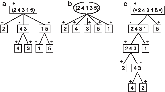
For example, let us consider the following circular genomes A = (2 4 3 1 5) and C = (1 2 3 4 5). The circular common intervals of A and C are {1, 5}, {1, 5, 2}, {4, 3}, {2, 4, 3}, and the singletons \documentclass{aastex}\usepackage{amsbsy}\usepackage{amsfonts}\usepackage{amssymb}\usepackage{bm}\usepackage{mathrsfs}\usepackage{pifont}\usepackage{stmaryrd}\usepackage{textcomp}\usepackage{portland, xspace}\usepackage{amsmath, amsxtra}\pagestyle{empty}\DeclareMathSizes{10}{9}{7}{6}\begin{document}$$\{1 \} \ldots \{5 \} $$\end{document} . The circular strong intervals are all the circular common intervals. The vertices of the circular common interval tree T (A, C) are {1, 5}, {4, 3} and the singletons. Remark that {1, 5, 2} and {2, 4, 3} are excluded from T (A, C) because they do not commute, although being circularly commuting. The tree T (A, C) is depicted in Figure 2a.

FIG. 2.

Let genomes A = (2 4 3 1 5), B = (2 4 1 3 5), and C = (1 2 3 4 5). (a) The circular common interval tree of genomes A and C. (b) The circular common interval tree of genomes B and C. (c) The strong interval tree of genomes (∘ 2 4 3 1 5 ∘) and (∘ 1 2 3 4 5 ∘). Rectangular nodes correspond to linear vertices and round nodes to prime vertices. The signs of linear vertices are indicated by a + or − symbol.

Given a vertex I of T (A, B), two orderings, either both circular, or both linear, of the set of children of I can be inferred from the orderings of the blocks in A and B corresponding to I. Following the notation of Bérard et al. (2007), the vertex I is linear if both orderings are identical or reciprocal, otherwise the vertex I is prime. If I is a linear vertex, I has a positive sign if both orderings are identical, and a negative sign if they are reciprocal (Fig. 2).

A circular common interval tree is definite if its vertices are linear. For example, in Figure 2, the left-hand tree (a) is definite, while the middle one (b) is not definite.

The definition of linear or prime vertices, and definite trees, also hold for the strong interval tree of two linear genomes (signed linear permutations). Given a vertex I of the strong interval tree of two linear genomes A and B, if I is linear (resp. prime), we also say that the common interval I between A and B is linear (resp. prime) Bérard et al. (2007) (Fig. 2c).

Ultra-perfect DCJ scenarios

In Bérard et al. (2007), it was shown that the existence of a perfect inversion scenario between unichromosomal linear genomes A and B was conditioned on properties of the strong interval tree of A and B: there exists a commuting scenario if and only if the strong interval tree is definite. In the following, we give the equivalent theorem for DCJ scenarios with circular common interval trees: there exists an ultra-perfect DCJ scenario if and only if the circular common interval tree is definite. We start by stating an obvious but useful property of ultra-perfect DCJ scenarios.

Property 1

Let A and B be unichromosomal genomes on the same set of blocks G. G is a common interval between A and B. So, if a DCJ scenario \documentclass{aastex}\usepackage{amsbsy}\usepackage{amsfonts}\usepackage{amssymb}\usepackage{bm}\usepackage{mathrsfs}\usepackage{pifont}\usepackage{stmaryrd}\usepackage{textcomp}\usepackage{portland, xspace}\usepackage{amsmath, amsxtra}\pagestyle{empty}\DeclareMathSizes{10}{9}{7}{6}\begin{document}$${\cal S}$$\end{document} from A to B is ultra-perfect, then any operation in \documentclass{aastex}\usepackage{amsbsy}\usepackage{amsfonts}\usepackage{amssymb}\usepackage{bm}\usepackage{mathrsfs}\usepackage{pifont}\usepackage{stmaryrd}\usepackage{textcomp}\usepackage{portland, xspace}\usepackage{amsmath, amsxtra}\pagestyle{empty}\DeclareMathSizes{10}{9}{7}{6}\begin{document}$${\cal S}$$\end{document} is either an inversion, or a circularization, or a linearization.

The circular version of a unichromosomal genome A is A itself if A is already a circular genome, otherwise it is the circular genome obtained by applying the circularization DCJ on A. We denote by A_c the circular version of a genome A.

Theorem 1

Let A and B be two unichromosomal genomes with the same set of blocks. There exists an ultra-perfect DCJ scenario from A to B if and only if the circular common interval tree of A_c and B_c is definite.

Proof

Let T = T(A_c, B_c) be a circular common interval tree of A_c and B_c.

First, if T is definite, then an inversion scenario \documentclass{aastex}\usepackage{amsbsy}\usepackage{amsfonts}\usepackage{amssymb}\usepackage{bm}\usepackage{mathrsfs}\usepackage{pifont}\usepackage{stmaryrd}\usepackage{textcomp}\usepackage{portland, xspace}\usepackage{amsmath, amsxtra}\pagestyle{empty}\DeclareMathSizes{10}{9}{7}{6}\begin{document}$${\cal S}$$\end{document} composed of inversions whose associated sets are the vertices of T that have a sign different from their parents is a commuting inversion scenario from A_c to B_c. So, \documentclass{aastex}\usepackage{amsbsy}\usepackage{amsfonts}\usepackage{amssymb}\usepackage{bm}\usepackage{mathrsfs}\usepackage{pifont}\usepackage{stmaryrd}\usepackage{textcomp}\usepackage{portland, xspace}\usepackage{amsmath, amsxtra}\pagestyle{empty}\DeclareMathSizes{10}{9}{7}{6}\begin{document}$${\cal S}$$\end{document} is an ultra-perfect scenario. Say e \documentclass{aastex}\usepackage{amsbsy}\usepackage{amsfonts}\usepackage{amssymb}\usepackage{bm}\usepackage{mathrsfs}\usepackage{pifont}\usepackage{stmaryrd}\usepackage{textcomp}\usepackage{portland, xspace}\usepackage{amsmath, amsxtra}\pagestyle{empty}\DeclareMathSizes{10}{9}{7}{6}\begin{document}$${\cal S}$$\end{document} f is the DCJ scenario from A to B where e is the eventual circularization transforming A into A_c and f is the eventual linearization transforming B_c into B. It is easy to see that e \documentclass{aastex}\usepackage{amsbsy}\usepackage{amsfonts}\usepackage{amssymb}\usepackage{bm}\usepackage{mathrsfs}\usepackage{pifont}\usepackage{stmaryrd}\usepackage{textcomp}\usepackage{portland, xspace}\usepackage{amsmath, amsxtra}\pagestyle{empty}\DeclareMathSizes{10}{9}{7}{6}\begin{document}$${\cal S}$$\end{document} f is an ultra-perfect scenario from A to B.

Now, if T is not definite, let I be a vertex of T that is prime. Since a DCJ scenario from A to B contains only inversions, circularization and linearization, then there exists no ultra-perfect DCJ scenario that sorts A_I into B_I. ▪

For example, consider the linear genomes A = (∘ 3 1 5 2 4 ∘) and B = (∘ 1 2 3 4 5 ∘). The circular common interval tree of the circular versions of A and B is depicted in Figure 2a. Since it is a definite tree, then there exists the following ultra-perfect DCJ scenario: \documentclass{aastex}\usepackage{amsbsy}\usepackage{amsfonts}\usepackage{amssymb}\usepackage{bm}\usepackage{mathrsfs}\usepackage{pifont}\usepackage{stmaryrd}\usepackage{textcomp}\usepackage{portland,xspace}\usepackage{amsmath,amsxtra}\pagestyle{empty}\DeclareMathSizes{10}{9}{7}{6}\begin{document}\begin{align*} \begin{array}{llll} (\circ \ 3 \ 1 \ 5 \ 2 \ 4 \ \circ) & circularization & (4 \ {- }5 \ {- }1 \ 2 \ 3) & inversion \ of \ \{1 \} \\ (3 \ 1 \ 5 \ 2 \ 4) & inversion \ of \ \{4 , 3 \} & (4 \ {- 5} \ 1 \ 2 \ 3) & inversion \ of \ \{5 \} \\ ({- 4} \ 1 \ 5 \ 2 {- 3}) & inversion \ of \ \{1 , 5 \} & (4 \ 5 \ 1 \ 2 \ 3) & linearization\\ ({- 4} \ {- 5} \ {- 1} \ 2 \ {- 3}) & inversion \ of \ \{4 \} & (\circ \ 1 \ 2 \ 3 \ 4 \ 5 \ {\circ}) & \\ (4 \ {- 5} \ {- 1} \ 2 \ {- 3}) & inversion \ of \ \{3\}& & \end{array} \end{align*}\end{document}

4. Ultra-perfection in practice

The number of datasets available to test the concept of ultra-perfection is currently very low. In this section, we study four of them. The first one goes back to early 20th century and documents inversions linking chromosomes of thirteen closely related drosophila flies. Almost none of the pairwise comparisons in this dataset are perfect or ultra-perfect, which underlies the apparent randomness of inversions in this group. The second dataset compares two drosophila species—D. melanogaster and D. yakuba—whose common ancestor dates back to more than 12 million years: one chromosome displays a remarkable ultra-perfect scenario. The third dataset comes from the comparison of the human chromosome 17 with the mouse chromosome 11, where a parsimonious ultra-perfect scenario of twelve inversions exists. Finally we discuss near ultra-perfection using the comparison of the human, mouse, and rat chromosome X.

4.1. Inversions in chromosome 3 of Drosophila pseudoobscura

In a landmark article on genome rearrangements, Dobzhansky and Sturtevant (1938) described a phylogeny of various strains of D. pseudoobscura using polytene chromosomes. These chromosomes exist in cells that undergo several rounds of DNA replication, without cell division, forming huge chromosomes with a characteristic banding patterns that reflects gene order.

Figure 3 shows the subtree that relates 13 strains, one of them predicted, in which each adjacent pair is separated by one inversion. We translated the gene orders into signed permutations on 19 blocks, with the identity permutation labeling the Standard arrangement. The edges are labeled by the set of blocks that are reversed. The topology of the tree is the unique parsimonious topology corresponding to reversals, due to the additivity of the pairwise distances.

FIG. 3.

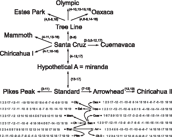
Phylogenetic tree of 13 strains of Drosophila flies. The relative gene order of the strains is modeled by signed permutations of 19 blocks. Each edge of the tree is labeled by the set of inverted blocks between two adjacent strains.

There are 66 pairwise scenarios of length 2 or more implied by the tree. Only 8 of the 21 scenarios of length 2 are ultra-perfect. Of the remaining scenarios none are ultra-perfect and 8 are perfect; 7 of which are trivially perfect as the first and last permutations are bereft of non-trivial common intervals. The exception is the comparison of strains Tree line and Pikes Peak. Table 1 gives the detailed results in terms of length of scenario between pairs of permutations.

Table 1.

Detailed Results

Length	n	Ultra-perfect	Perfect	Trivial
2	21	8	8	0
3	20	0	1	1
4	12	0	3	2
5	10	0	4	4
6	3	0	0	0

This example clearly illustrates ultra-perfection as an uncommon feature of inversion scenarios. Random inversions, even those that disrupt clusters of co-expressed genes, are possible (Meadows et al., 2010), and it takes only a few overlapping inversions to lose common intervals. Herein lies the significance of identifying ultra-perfect scenarios.

4.2. Comparing chromosomes 3R of D. melanogaster and D. yakuba

The next dataset comes from the 12 Drosophila sequencing project and is based on the breakpoints and inversions identified between the 3R chromosomes of D. yakuba and D. melanogaster Schaeffer et al. (2008); Ranz et al. (2007). In Schaeffer et al. (2008), the authors identify 9 inversions separating the two species, and analysis of their suggested 12 breakpoints yields the signed permutations: \documentclass{aastex}\usepackage{amsbsy}\usepackage{amsfonts}\usepackage{amssymb}\usepackage{bm}\usepackage{mathrsfs}\usepackage{pifont}\usepackage{stmaryrd}\usepackage{textcomp}\usepackage{portland,xspace}\usepackage{amsmath,amsxtra}\pagestyle{empty}\DeclareMathSizes{10}{9}{7}{6}\begin{document}\begin{align*} Dmel & = \ (\circ \ 1 \ 2 \ 3 \ 4 \ 5 \ 6 \ 7 \ 8 \ 9 \ 10 \ 11 \ 12 \ 13 \ {\circ}) \\ Dyak & = \ (\circ \ 1 \ 10 \ {- 3} \ 4 \ {- 8} \ 6 \ {- 7} \ {- 5} \ 9 \ 2 \ 11 \ {- 12} \ 13 \ {\circ} ). \end{align*}\end{document}

Figure 4a gives the strong intervals tree resulting from the comparison of those two permutations: it contains only linear vertices and indicates an ultra-perfect scenario of length 9, obtained by inverting the sets in the shaded vertices of the tree. This scenario corresponds to that proposed in Schaeffer et al. (2008). In Ranz et al. (2007), the authors propose a parsimonious scenario of length 7, depicted in Figure 4b. This scenario is based not only on parsimony, but also on additional genomic information used by the authors to perform mandatory inversions.

FIG. 4.

(a) The strong intervals tree resulting from the comparison of chromosomes 3R of D. melanogaster and D. Yakuba. Reversing the intervals corresponding to shaded blocks yield an ultra-perfect scenario of length 9 proposed in Schaeffer et al. (2008). (b) The parsimonious scenario of length 7 proposed in Ranz et al. (2007).

4.3. The human chromosome 17 and the mouse chromosome 11

The comparison between the human chromosome 17 with the mouse genome reveals that the whole human chromosome is syntenic with a major section of mouse chromosome 11 (Bourque et al., 2004). Comparison of the blocks common in human, rat and mouse, yields the following permutations for the human and mouse: \documentclass{aastex}\usepackage{amsbsy}\usepackage{amsfonts}\usepackage{amssymb}\usepackage{bm}\usepackage{mathrsfs}\usepackage{pifont}\usepackage{stmaryrd}\usepackage{textcomp}\usepackage{portland,xspace}\usepackage{amsmath,amsxtra}\pagestyle{empty}\DeclareMathSizes{10}{9}{7}{6}\begin{document}\begin{align*} H17 & = \ (\circ \ 1 \ 2 \ 3 \ 4 \ 5 \ 6 \ 7 \ 8 \ 9 \ 10 \ 11 \ 12 \ 13 \ 14 \ 15 \ 16 \ 17 \ 18 \ 19 \ {\circ}) \\ M11 & = \ (\circ \ 7 \ {- 8} \ 6 \ {- 5} \ 4 \ {- 3} \ 1 \ 2 \ {- 10} \ {- 9} \ 11 \ 12 \ {- 13} \ 16 \ {- 15} \ 14 \ 17 \ {- 18} \ 19 \ {\circ}) \end{align*}\end{document}

The most striking feature of these permutations is the existence of an ultra-perfect scenario that is also most parsimonious. Figure 5 displays this scenario, of length 12, as shaded vertices of the corresponding strong intervals tree.

FIG. 5.

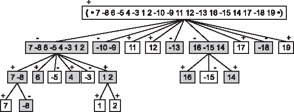
The strong intervals tree resulting from the comparison of human chromosome 17 and mouse chromosome 11. Reversing the intervals corresponding to shaded blocks yield an ultra-perfect scenario of length 12. This scenario is also parsimonious.

For these two permutations, there exist other parsimonious sorting scenarios that are not ultra-perfect. These scenarios can be partitioned into 21 distinct traces computed with baobabLUNA (Braga, 2009). (For further detail, see online Supplementary Material at www.liebertonline.com/cmb.) Figure 6 displays, side-by-side, the segment of permutations M11 and H17 containing blocks 1 to 10 sorted by a non ultra-perfect scenario and by an ultra-perfect scenario, showing the disruption of gene synteny.

FIG. 6.

Two parsimonious scenarios that sort the segment of permutations M11 and H17 containing blocks 1 to 10. The scenario on the right is ultra-perfect, and the scenario on the left is not.

4.4. Imperfect sorting

When no ultra-perfect scenario exists, we wish to define a way to score scenarios that are nearly ultra-perfect. There is no easy or straightforward way to do this: the competing parameters include broken common intervals, overlapping inversions, prime intervals and parsimony. In this section, we propose a first measure that is relatively simple to define, and that allows us to compare scenarios that would otherwise be difficult to rank.

Our first simplification is that, when trying to build a scenario for two or more species, each common interval should be sorted independently. Since linear common intervals are rather easy to sort with an ultra-perfect scenario, we focus on the sorting of individual prime common intervals.

A scenario \documentclass{aastex}\usepackage{amsbsy}\usepackage{amsfonts}\usepackage{amssymb}\usepackage{bm}\usepackage{mathrsfs}\usepackage{pifont}\usepackage{stmaryrd}\usepackage{textcomp}\usepackage{portland, xspace}\usepackage{amsmath, amsxtra}\pagestyle{empty}\DeclareMathSizes{10}{9}{7}{6}\begin{document}$${\cal S}$$\end{document} between two or more species can be represented as an unrooted tree whose nodes are the genomes, and whose branches are the rearrangement operations. Removing an operation r from a scenario \documentclass{aastex}\usepackage{amsbsy}\usepackage{amsfonts}\usepackage{amssymb}\usepackage{bm}\usepackage{mathrsfs}\usepackage{pifont}\usepackage{stmaryrd}\usepackage{textcomp}\usepackage{portland, xspace}\usepackage{amsmath, amsxtra}\pagestyle{empty}\DeclareMathSizes{10}{9}{7}{6}\begin{document}$${\cal S}$$\end{document} is done by cutting the branch labeled by r yielding two subtrees called subscenarios. We have:

Definition 4

The imperfection score of a scenario \documentclass{aastex}\usepackage{amsbsy}\usepackage{amsfonts}\usepackage{amssymb}\usepackage{bm}\usepackage{mathrsfs}\usepackage{pifont}\usepackage{stmaryrd}\usepackage{textcomp}\usepackage{portland, xspace}\usepackage{amsmath, amsxtra}\pagestyle{empty}\DeclareMathSizes{10}{9}{7}{6}\begin{document}$${\cal S}$$\end{document} is the minimum number of operations that can be removed from \documentclass{aastex}\usepackage{amsbsy}\usepackage{amsfonts}\usepackage{amssymb}\usepackage{bm}\usepackage{mathrsfs}\usepackage{pifont}\usepackage{stmaryrd}\usepackage{textcomp}\usepackage{portland, xspace}\usepackage{amsmath, amsxtra}\pagestyle{empty}\DeclareMathSizes{10}{9}{7}{6}\begin{document}$${\cal S}$$\end{document} such that each of the remaining subscenarios is ultra-perfect.

Our goal is to find, among all possible scenarios with minimum imperfection score, one that is of minimum length.

It turns out that the data on human, mouse, and rat chromosomes X is a very interesting instance of this problem: there are prime common intervals in both the Human-Mouse and the Human-Rat strong interval trees. The prime common interval in the Human-Mouse comparison is maximal, but there is no ultra-perfect scenario since the induced permutation from Bérard et al. (2007), (∘ −4 6 1 −3 −5 2 ∘), does not have a commuting scenario, even with circularization.

The following permutations, obtained from the blocks of Bourque et al. (2004), model the homologous blocks of the human, mouse, and rat chromosomes X: \documentclass{aastex}\usepackage{amsbsy}\usepackage{amsfonts}\usepackage{amssymb}\usepackage{bm}\usepackage{mathrsfs}\usepackage{pifont}\usepackage{stmaryrd}\usepackage{textcomp}\usepackage{portland,xspace}\usepackage{amsmath,amsxtra}\pagestyle{empty}\DeclareMathSizes{10}{9}{7}{6}\begin{document}\begin{align*} H & = \ (\circ \ 1 \ 2 \ 3 \ 4 \ 5 \ 6 \ 7 \ 8 \ 9 \ 10 \ 11 \ 12 \ 13 \ 14 \ 15 \ 16 \ {\circ}) \\ M & = \ (\circ \ {- 6} \ {- 5} \ 4 \ 13 \ 14 {- 15} \ 16 \ 1 \ {- 3} \ 9 \ {- 10} \ 11 \ 12 \ {- 7} \ 8 \ {- 2} \ {\circ}) \\ R & = \ (\circ \ {- 13} \ {- 4} \ 5 \ {- 6} \ {- 12} \ {- 8} \ {- 7} \ 2 \ 1 \ {- 3} \ 9 \ 10 \ 11 \ 14 \ {- 15} \ 16 \ {\circ}) \end{align*}\end{document}

We first apply single block inversions (they have no impact on the perfection of a scenario) that create an adjacency in one genome that already exists in the other two. There are 5 of them in the chromosome data: {4} and {15} applied to the human chromosome, {7} and {10} applied to the mouse chromosome, and {6} applied to the rat chromosome. The resulting chromosomes are the following, renamed with a subscript that indicates how far the new chromosome is from the original. \documentclass{aastex}\usepackage{amsbsy}\usepackage{amsfonts}\usepackage{amssymb}\usepackage{bm}\usepackage{mathrsfs}\usepackage{pifont}\usepackage{stmaryrd}\usepackage{textcomp}\usepackage{portland,xspace}\usepackage{amsmath,amsxtra}\pagestyle{empty}\DeclareMathSizes{10}{9}{7}{6}\begin{document}\begin{align*} H_{+ 2} & = \ (\circ \ 1 \ 2 \ 3 \ {- 4} \ 5 \ 6 \ 7 \ 8 \ 9 \ 10 \ 11 \ 12 \ 13 \ 14 \ {- 15} \ 16 \ {\circ}) \\ M_{+ 2} & = \ (\circ \ {- 6} \ {- 5} \ 4 \ 13 \ 14 \ {- 15} \ 16 \ 1 \ {- 3} \ 9 \ {10} \ 11 \ 12 \ {7} \ 8 \ {- 2} \ {\circ}) \\ R_{+ 1} & = \ (\circ \ {- 13} \ {- 4} \ 5 \ {6} \ {- 12} \ {- 8} \ {- 7} \ 2 \ 1 \ {- 3} \ 9 \ 10 \ 11 \ 14 \ {- 15} \ 16 \ {\circ}) \end{align*}\end{document}

Next, there are three adjacencies that are shared by the rodents, but are not in the human lineage, and that require inversions longer than single blocks: (1 − 3), (4 13) and (−3 9). The corresponding inversions associated to the sets, {2, 3},{4, 5, 6, 7, 8, 9, 10, 11, 12} and {2, 9, 10, 11, 12} can be applied to the H₊₂ genome to yield H₊₅ = (∘ 1 −3 9 10 11 12 2 −8 −7 −6 −5 4 13 14 −15 16 ∘).

In the next section, we will construct an ultra-perfect scenario for the three permutations H₊₅, M₊₂ and R₊₁. Since the first two inversions applied to the H₊₂ chromosome are commuting, the imperfection score of the global scenario will be 1, obtained by removing inversion {2, 9, 10, 11, 12}, which is the best that can be achieved. The scenario between H₊₂ and H₊₅ is also parsimonious, since it constructs 3 adjacencies present in both the mouse and rat genome, implying that any alternate solution should have the same length. Up to commutation of the two initial inversions, it is easy to show that this is the only solution constructing the 3 adjacencies.

4.5. The ultra-perfect median of three genomes

After applying the inversions of the preceding section, the three genomes are the following, where adjacencies common to all three chromosomes are indicated by dots: \documentclass{aastex}\usepackage{amsbsy}\usepackage{amsfonts}\usepackage{amssymb}\usepackage{bm}\usepackage{mathrsfs}\usepackage{pifont}\usepackage{stmaryrd}\usepackage{textcomp}\usepackage{portland,xspace}\usepackage{amsmath,amsxtra}\pagestyle{empty}\DeclareMathSizes{10}{9}{7}{6}\begin{document}\begin{align*} H_{+ 5} & = \ (\circ \ 1 \cdot {- 3} \cdot 9 \cdot 10 \cdot 11 \ 12 \ 2 \ {- 8} \cdot{- 7} \ {- 6} \cdot{- 5} \cdot 4 \cdot13 \ \ 14 \cdot {- 15} \cdot 16 \ {\circ}) \\ M_{+ 2} & = \ (\circ \ {- 6} \cdot{- 5} \cdot 4 \cdot13 \ 14 \cdot {- 15} \cdot 16 \ 1 \cdot {- 3} \cdot 9 \cdot 10 \cdot 11 \ 12 \ 7 \cdot 8 \ {- 2} \ {\circ}) \\ R_{+ 1} & = \ (\circ \ {- 13} \cdot{- 4} \cdot5 \cdot6 \ {- 12} \ {- 8} \cdot{- 7} \ 2 \ 1 \cdot{- 3} \cdot9 \cdot10 \cdot11 \ 14 \cdot{- 15} \cdot 16 \ {\circ}) \end{align*}\end{document}

It is convenient, at this point, to relabel the blocks so that the remaining differences are more apparent. There are six blocks that we label with respect to the H₊₅ genome order: \documentclass{aastex}\usepackage{amsbsy}\usepackage{amsfonts}\usepackage{amssymb}\usepackage{bm}\usepackage{mathrsfs}\usepackage{pifont}\usepackage{stmaryrd}\usepackage{textcomp}\usepackage{portland,xspace}\usepackage{amsmath,amsxtra}\pagestyle{empty}\DeclareMathSizes{10}{9}{7}{6}\begin{document}\begin{align*} \overbrace{1 \cdot {- 3} \cdot 9 \cdot 10 \cdot 11}^{\bf{1}} \overbrace{12}^{\bf{2}} \overbrace{2}^{\bf{3}} \overbrace{{- 8} \cdot{- 7}}^{\bf{4}} \overbrace{{- 6} \cdot{- 5} \cdot 4 \cdot13}^{\bf{5}} \overbrace{14 \cdot {- 15} \cdot 16}^{\bf{6}} \end{align*}\end{document}

This yields the new representation: \documentclass{aastex}\usepackage{amsbsy}\usepackage{amsfonts}\usepackage{amssymb}\usepackage{bm}\usepackage{mathrsfs}\usepackage{pifont}\usepackage{stmaryrd}\usepackage{textcomp}\usepackage{portland,xspace}\usepackage{amsmath,amsxtra}\pagestyle{empty}\DeclareMathSizes{10}{9}{7}{6}\begin{document}\begin{align*} H_{+ 5} & = \ (\circ \ \bf{1 \ 2 \ 3 \ 4 \ 5 \ 6} \ {\circ}) \\ M_{+ 2} & = \ (\circ \ \bf{5 \ 6 \ 1 \ 2 \ {- 4} \ {- 3}} \ {\circ}) \\ R_{+ 1} & = \ (\circ \ \bf{{- 5} \ {- 2} \ 4 \ 3 \ 1 \ 6} \ {\circ}) \end{align*}\end{document}

Given three genomes, deciding if an ultra-perfect scenario connecting them exists begins with a simple check. Indeed, the median of three genomes belongs to all implied pairwise scenarios, thus must share all common intervals of all pairs of genomes. Formally we have:

Proposition 3

The median M of an ultra-perfect scenario linking three permutations A, B and C contains all common intervals of A and B, of A and C, and of B and C.

In order to apply Proposition 3 to the mammal chromosomes, we first compute their common intervals: \documentclass{aastex}\usepackage{amsbsy}\usepackage{amsfonts}\usepackage{amssymb}\usepackage{bm}\usepackage{mathrsfs}\usepackage{pifont}\usepackage{stmaryrd}\usepackage{textcomp}\usepackage{portland,xspace}\usepackage{amsmath,amsxtra}\pagestyle{empty}\DeclareMathSizes{10}{9}{7}{6}\begin{document}\begin{align*} H_{+ 5} & \ {\rm and} \ M_{+ 2} : \ \bf{\{1 , 2 \} , \{3 , 4 \} , \{5 , 6 \} , \{2 , 3 , 4 \} , \{1 , 2 , 3 , 4 \} } \\ H_{+ 5} & \ {\rm and} \ R_{+ 1} : \bf{\{3 , 4 \} , \{2 , 3 , 4 \} , \{1 , 2 , 3 , 4 \} , \{2 , 3 , 4 , 5 \} , \{1 , 2 , 3 , 4 , 5 \} } \\ M_{+ 2} & \ {\rm and} \ R_{+ 1} : \bf{\{1 , 6 \} , \{2 , 4 \} , \{3 , 4 \} , \{2 , 3 , 4 \} , \{1 , 2 , 3 , 4 \} , \{1 , 2 , 3 , 4 , 6 \} } \end{align*}\end{document}

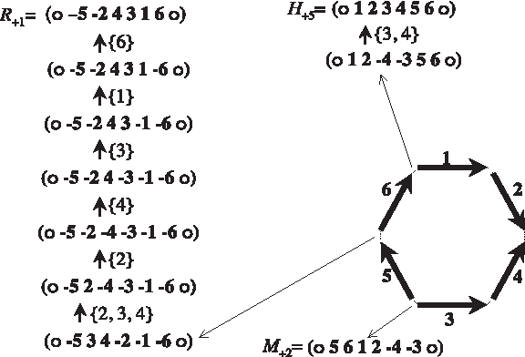
The—unique—permutation that contains all these intervals is a circular chromosome! Its block order, (5 6 1 2 −4 −3), is the circularization of the mouse genome. It is then a simple exercise to transform the median into each genome. The whole scenario has 7 inversions, 5 of them inverting single blocks; the remaining 2 inversions are {3, 4} towards the human chromosome, and {2, 3, 4} towards the rat chromosome (Fig. 7).

FIG. 7.

An ultra-perfect scenario between chromosomes H₊₅, M₊₂ and R₊₁. The location where the circular median is cut is shown by thin arrows. The set of inverted blocks is shown between each pair of permutations.

5. Conclusion

In this article, we showed that reality is seldom perfect or ultra-perfect, but some comparisons yield surprising results. When inversions occur in a seemingly random way, as in the dataset on drosophila strains, very few common intervals are found, even for close species. The comparison between D. melanogaster and D. yakuba has an ultra-perfect scenario that is not parsimonious, and up to the exchange of commuting inversions, a unique parsimonious scenario. In this case, it is interesting to note that both these scenarios are proposed in the literature. We also found an ultra-perfect scenario, involving the complete human chromosome 17, that is also parsimonious. This, together with the fact that gene synteny is conserved on an unusually large scale, is notable.

The search for an ultra-perfect scenario for the human, mouse, and rat X chromosome leads to a surprising circular median, deduced by combinatorial techniques. We are certainly not inferring that actual species had circular X chromosomes. The fact that the number of blocks is quite small, n = 6, might be the simplest explanation: more than half of the random trios of permutations on six elements have a circular median. However, the remarkable preservation of the circular order of blocks between the human and mouse X chromosome asks for a more satisfying answer. Are there some biological mechanisms that would allow rearrangement operations that preserve a circular order? Among the well known combinatorial operations with this property are the shift operation, or a double centromeric inversion.

On the algorithmic side, the circular common interval tree allows us to easily find the set of inversions of an ultra-perfect scenario between two genomes; ultra-perfect DCJ scenarios are essentially ultra-perfect inversion scenarios on a circular version of the genomes. In the case of multiple genomes, the existence and computation of an ultra-perfect scenario should be easy to characterize using the sets of inversions corresponding to pairwise genomes. In the case of nearly ultra-perfect scenario, methods still have to be developed but most efforts will likely lead to hardness results. However, interesting instances of the problem, such as rearrangements between human and rodents, are still quite manageable by manual techniques, and should get easier with the sequencing of additional rodent genomes. It is also relatively easy to score scenarios: the scenario proposed by GRIMM (Tesler, 2002) for the human, mouse and rat chromosome X has an imperfection score of 2.

Footnotes

Disclosure Statement

No competing financial interests exist.

References

Bérard

, Bergeron

, Chauve

2004. Conservation of combinatorial structures in evolution scenarios. Lect. Notes Comput. Sci., 3388:1–14.

Bérard

, Bergeron

, Chauve

et al. 2007. Perfect sorting by reversals is not always difficult. IEEE/ACM Trans. Comput. Biol. Bioinform., 4:4–16.

Bérard

, Chateau

, Chauve

et al. 2008. Perfect DCJ rearrangement. Lect. Notes Comput. Sci., 5267:158–169.

Bergeron

, Chauve

, de Montgolfier

et al. 2005. Computing common intervals of k permutations, with applications to modular decomposition of graphs. Lect. Notes Comput. Sci., 3669:779–790.

Bourque

, Pevzner

P.A.

, Tesler

2004. Reconstructing the genomic architecture of ancestral mammals: lessons from human, mouse, and rat genomes. Genome Res., 14:507–516.

Braga

M.D.

2009. baobabLUNA: the solution space of sorting by reversals. Bioinformatics, 25:1833–1835.

Braga

M.D.

, Gautier

, Sagot

M.-F.

2009. An asymmetric approach to preserve common intervals while sorting by reversals. Proc. Algorithms Mol. Biol., 4.

Dobzhansky

, Sturtevant

1938. Inversions in the chromosomes of Drosophila pseudoobscura. Genetics, 23:28–64.

Figeac

, Varré

J.-S.

2004. Sorting by reversals with common intervals. Lect. Notes Comput. Sci., 3240:26–37.

10.

Heber

, Stoye

2001. Finding all common intervals of k permutations. Lect. Notes Comput. Sci., 2089:207–218.

11.

Hsu

W.-L.

2001. PC-trees vs. PQ-trees. Lect. Notes in Comput. Sci., 2108:207–217.

12.

Hsu

W.-L.

, McConnell

R.M.

2003. PC trees and circular-ones arrangements. Theor. Comput. Sci., 296:99–116.

13.

Landau

G.M.

, Parida

, Weimann

2005. Using PQ trees for comparative genomics. Lect. Notes Comput. Sci., 3537:128–143.

14.

Meadows

L.A.

, Chan

Y.S.

, Roote

et al. 2010. Neighbourhood continuity is not required for correct testis gene expression in drosophila. PLoS Biol., 8:e1000552.

15.

Ranz

J.M.

, Maurin

, Chan

Y.S.

et al. 2007. Principles of genome evolution in the Drosophila melanogaster species group. PLoS Biol., 5:e152+.

16.

Sagot

M.-F.

, Tannier

2005. Perfect sorting by reversals. Lect. Notes Comput. Sci., 3595:42–51.

17.

Schaeffer

S.W.

, Bhutkar

, McAllister

B.F.

et al. 2008. Polytene chromosomal maps of 11 drosophila species: the order of genomic scaffolds inferred from genetic and physical maps. Genetics, 179:1601–1655.

18.

Tesler

2002. GRIMM: genome rearrangements web server. Bioinformatics, 18:492–493.

Supplementary Material

Please find the following supplemental material available below.

For Open Access articles published under a Creative Commons License, all supplemental material carries the same license as the article it is associated with.

For non-Open Access articles published, all supplemental material carries a non-exclusive license, and permission requests for re-use of supplemental material or any part of supplemental material shall be sent directly to the copyright owner as specified in the copyright notice associated with the article.

0.00 MB

0.02 MB