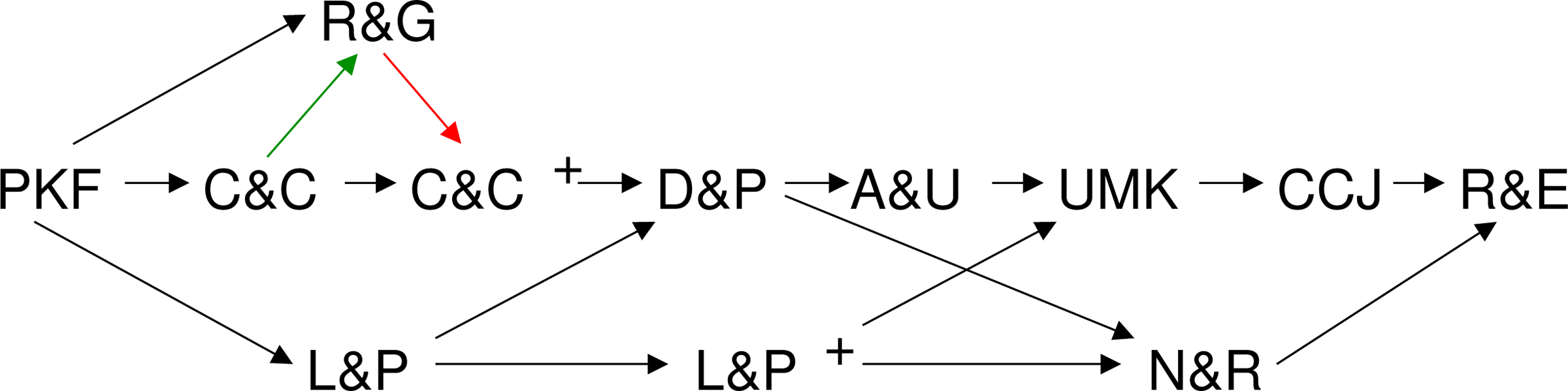
Predicting RNA structures with pseudoknots in general is an NP-complete problem. Accordingly, several authors have suggested subclasses that provide polynomial time prediction algorithms by allowing (respectively, disallowing) certain structural motives. In this article, we introduce a unifying algebraic view on most of these classes. That way it becomes possible to find linear time recognition algorithms that decide whether or not a given structure is member of a class (we offer these algorithms as a web service to the scientific community). Furthermore, by presenting a general translation scheme of our algebraic descriptions into multiple context-free grammars, and proving a new correspondence of multiple context-free grammars and generating functions, it becomes possible to derive the precise asymptotic size of all the classes, solving some open problems such as enumerating the Rivas & Eddy class of pseudoknots.
1. Introduction
To a large extent the function of an RNA molecule is determined by its secondary structure, that is, by the mutual arrangements of the base-paired helices. In this context however, secondary structure has to be understood in a wider sense by allowing pseudoknots. Even though the vast majority of RNAs has simple (i.e., pseudoknot-free) secondary structure, PseudoBase (Taufer et al., 2009) lists more than 300 records of pseudoknots determined by a variety of experimental and computational techniques, including crystallography, NMR spectroscopy, mutational experiments, and comparative sequence analysis. If present, pseudoknots, in many cases, are crucial for molecular function. Examples include the catalytic cores of several ribozymes (Doudna and Cech, 2002), telomerase activity (Theimer et al., 2005), reviewed in Staple and Butcher (2005) and Giedroc and Cornish (2009), and programmed frameshifting (Namy et al., 2006). Accordingly, one aims for in silico prediction of RNA structure, which unfortunately has been proven \documentclass{aastex}\usepackage{amsbsy}\usepackage{amsfonts}\usepackage{amssymb}\usepackage{bm}\usepackage{mathrsfs}\usepackage{pifont}\usepackage{stmaryrd}\usepackage{textcomp}\usepackage{portland, xspace}\usepackage{amsmath, amsxtra}\pagestyle{empty}\DeclareMathSizes{10}{9}{7}{6}\begin{document}
$${\cal NP}$$
\end{document}-complete when allowing unrestricted conformations, even under the assumption of rather simple energy models (Akutsu, 2000; Lyngsø and Pedersen, 2000b). However, polynomial-time algorithms have been devised for certain restricted classes of pseudoknots. The following references provide a certainly incomplete list of those approaches: Akutsu (2000); Cao and Chen (2009); Chen et al. (2009); Dirks and Pierce (2003); Kato et al. (2006); Lyngsø and Pedersen (2000a); Matsui et al. (2005); Reeder and Giegerich (2004); Reidys et al. (2011); Rivas and Eddy (1999); and Uemura Y. et al. (1999). The interrelationships of some of these classes have been partially clarified by Condon et al. (2004) and Rødland (2006). Furthermore, Saule et al. (2011) presents enumeration results quantifying the size of some of those classes. In addition to the previously mentioned exact algorithms, plenty of heuristic approaches to pseudoknot prediction have been suggested; see, e.g., Chen (2008), Metzler and Nebel (2008), and the references therein.
In this contribution, we provide a unified algebraic characterization of all the before-mentioned classes connected to exact approaches. For this purpose, we make use of operators like nesting or stem extension to show how each class can be understood as the smallest set of conformations closed under a properly chosen combination of operators. This way, it is possible to understand the interrelations between the classes, proving inclusion or incomparability. Additionally, we are able to derive linear time recognition algorithms for all the classes. To the best of our knowledge, those have not been available in all cases so far. Furthermore, we show how all the operators used can be translated into unambiguous multiple context-free grammars (MCFG). As a consequence, grammar representations for all the pseudoknot classes are found. By proving a new enumeration lemma that allows for computing the number of different words of length n in the language generated by any unambiguous MCFG, we are able to provide exact asymptotics for the sizes of all the classes. This way, we are able to provide the first results for the size of Rivas & Eddy's pseudoknot class, solving a problem now open for more than 10 years.
2. Definitions of Pseudoknot Classes
2.1. The pseudoknot free (PKF) class
For completeness, we also include the class of pseudoknot free secondary structures in our treatment. It is easily verified that any such structure can be created by taking a number of base pairs and unpaired bases and concatenate or embed them into the growing structure. Note that we assume in the entirety of this article a minimal hairpin loop length of zero. This is no restriction implied by our ideas or methods but helps to reduce the complexity of the presentation.
2.2. The Rivas and Eddy (R&E) class
In Rivas and Eddy (1999) an extension of the traditional dynamic programming scheme of Zuker and Stiegler (1981) is introduced, which allows for predicting a huge class of pseudoknots.
The original algorithm basically determines the optimal folding for any connected region of the RNA molecule by considering either adding a pairing consisting of the first and last base of the region to the optimal folding of the remaining region, or splitting it into two smaller connected regions for which the optimal folding has been determined earlier. As a base case, regions of size 1 always consist of a single unpaired nucleotide.
The new algorithm additionally considers regions that are not entirely connected but have a single gap inside. Figure 1 shows the different ways a connected or gapped region may be decomposed into two gapped regions. Here the horizontal lines show (segments of) the backbone of the molecule and a semi-disc in the upper (respectively, lower) half-plane is used to represent a gapped region where the inner half-circle determines the gap and the positions between the two circles may be paired. Additionally, the algorithm can decompose a gapped region into a gapped and a connected region in all 4 possible ways, and it may decompose a gapped region into two separate connected regions. The base case for gapped regions is a single base pair.
Decomposing a connected or gapped region into two gapped regions.
The algorithm works in \documentclass{aastex}\usepackage{amsbsy}\usepackage{amsfonts}\usepackage{amssymb}\usepackage{bm}\usepackage{mathrsfs}\usepackage{pifont}\usepackage{stmaryrd}\usepackage{textcomp}\usepackage{portland, xspace}\usepackage{amsmath, amsxtra}\pagestyle{empty}\DeclareMathSizes{10}{9}{7}{6}\begin{document}
$${\cal O} (n^{6})$$
\end{document} time and \documentclass{aastex}\usepackage{amsbsy}\usepackage{amsfonts}\usepackage{amssymb}\usepackage{bm}\usepackage{mathrsfs}\usepackage{pifont}\usepackage{stmaryrd}\usepackage{textcomp}\usepackage{portland, xspace}\usepackage{amsmath, amsxtra}\pagestyle{empty}\DeclareMathSizes{10}{9}{7}{6}\begin{document}
$${\cal O} (n^{4})$$
\end{document} space. While it is known that the class of pseudoknots that can be predicted by it (called R&E) is a superclass of any other class for which an exact prediction algorithm has been suggested thus far, and Condon et al. (2004) gives a linear time algorithm that decides if a given structure is in R&E, neither the size of the class nor a short description of it (e.g., as a formal language) has been determined so far.
2.3. The Uemura et al. (UMK) class
In Uemura et al. (1999), a set of rules for tree-adjoined grammars is suggested that can be used to generate a language that models pseudoknots. In Matsui et al. (2005), these rules are translated into the setting of pair-stochastic tree-adjoined grammar. In Kato et al. (2006), an equivalent set of rules for stochastic multiple context-free grammars is given. All algorithms run in \documentclass{aastex}\usepackage{amsbsy}\usepackage{amsfonts}\usepackage{amssymb}\usepackage{bm}\usepackage{mathrsfs}\usepackage{pifont}\usepackage{stmaryrd}\usepackage{textcomp}\usepackage{portland, xspace}\usepackage{amsmath, amsxtra}\pagestyle{empty}\DeclareMathSizes{10}{9}{7}{6}\begin{document}
$${\cal O} (n^{5})$$
\end{document} time and \documentclass{aastex}\usepackage{amsbsy}\usepackage{amsfonts}\usepackage{amssymb}\usepackage{bm}\usepackage{mathrsfs}\usepackage{pifont}\usepackage{stmaryrd}\usepackage{textcomp}\usepackage{portland, xspace}\usepackage{amsmath, amsxtra}\pagestyle{empty}\DeclareMathSizes{10}{9}{7}{6}\begin{document}
$${\cal O} (n^{4})$$
\end{document} space.
The construction of a secondary structure according to this set of rules can be viewed as starting with two insertion points and repeatedly inserting a base pair with one of its bases to the immediate left of one insertion point, and the other base to the immediate right of either the same or the other insertion point. Additionally, unpaired bases or substructures (of the same type) may be inserted at either point.
Thus, a single UMK structure element consists of three groups of base pairs, each of which may be empty. Within each group, all base pairs form a possibly interrupted stem, i.e., are nested as in the second picture of Figure 1, possibly with bases from other groups between them. The left and right group of base pairs do not overlap, and there is a position between these groups such that all base pairs in the middle group span this position. See Figure 2 for an example. An UMK structure then consists of any number of UMK structure elements arbitrarily concatenated and embedded inside each other.
A UMK-pseudoknot.
For this class, no previous results concerning the size or a linear time recognition algorithm or relation to other classes except R&E are known to the authors.
2.4. The Akutsu and Uemura (A&U) class
In Akutsu (2000), a minimum free energy–based dynamic programming algorithm is proposed that predicts pseudoknots from a subclass of UMK in \documentclass{aastex}\usepackage{amsbsy}\usepackage{amsfonts}\usepackage{amssymb}\usepackage{bm}\usepackage{mathrsfs}\usepackage{pifont}\usepackage{stmaryrd}\usepackage{textcomp}\usepackage{portland, xspace}\usepackage{amsmath, amsxtra}\pagestyle{empty}\DeclareMathSizes{10}{9}{7}{6}\begin{document}
$${\cal O} (n^{5})$$
\end{document} time.
A&U structures are built from so-called simple pseudoknots. A simple pseudoknot consists of two groups of base pairs, the base pairs of each group forming a stem. Base pairs are arranged such that the right bases of the first group and the left bases of the second group are interleaved arbitrarily, while the other bases all lie outside of the interleaved area. See Figure 3 for an example.
A simple pseudoknot (left) and an H-type pseudoknot (right).
An A&U structure then consists of any number of pseudoknot free structures and simple pseudoknots arbitrarily concatenated and embedded inside each other.
The inclusion relation of A&U with most of the other classes has been examined in Condon et al. (2004) and extended in Saule et al. (2011), where additionally its size was determined. A linear time recognition algorithm, however, has not yet been given.
2.5. The Lyngsø and Pedersen (L&P, L&P+) classes
In Lyngsø and Pedersen (2000a), an algorithm based on the minimum free energy paradigm is presented that runs in \documentclass{aastex}\usepackage{amsbsy}\usepackage{amsfonts}\usepackage{amssymb}\usepackage{bm}\usepackage{mathrsfs}\usepackage{pifont}\usepackage{stmaryrd}\usepackage{textcomp}\usepackage{portland, xspace}\usepackage{amsmath, amsxtra}\pagestyle{empty}\DeclareMathSizes{10}{9}{7}{6}\begin{document}
$${\cal O} (n^{5})$$
\end{document} time and \documentclass{aastex}\usepackage{amsbsy}\usepackage{amsfonts}\usepackage{amssymb}\usepackage{bm}\usepackage{mathrsfs}\usepackage{pifont}\usepackage{stmaryrd}\usepackage{textcomp}\usepackage{portland, xspace}\usepackage{amsmath, amsxtra}\pagestyle{empty}\DeclareMathSizes{10}{9}{7}{6}\begin{document}
$${\cal O} (n^{3})$$
\end{document} space and predicts structures in the form w1u1w2u2w3, where w1w2w3 and u1u2 are arbitrary pseudoknot free structures. This class of structures is labeled as L&P+ in Condon et al. (2004). Additionally, Condon et al. (2004) also defines the subclass of structures w1u1w2u2, w1w2 and u1u2 pseudoknot free, and labels that class as L&P.
For L&P, Condon et al. (2004) gives a linear time recognition algorithm along with some inclusion results, and Saule et al. (2011) extends the inclusion results and gives the size of the class. L&P+ has not yet been further examined.
2.6. The Dirks and Pierce (D&P) class
In Dirks and Pierce (2003), a dynamic programming algorithm is introduced that runs in \documentclass{aastex}\usepackage{amsbsy}\usepackage{amsfonts}\usepackage{amssymb}\usepackage{bm}\usepackage{mathrsfs}\usepackage{pifont}\usepackage{stmaryrd}\usepackage{textcomp}\usepackage{portland, xspace}\usepackage{amsmath, amsxtra}\pagestyle{empty}\DeclareMathSizes{10}{9}{7}{6}\begin{document}
$${\cal O} (n^{5})$$
\end{document} time and \documentclass{aastex}\usepackage{amsbsy}\usepackage{amsfonts}\usepackage{amssymb}\usepackage{bm}\usepackage{mathrsfs}\usepackage{pifont}\usepackage{stmaryrd}\usepackage{textcomp}\usepackage{portland, xspace}\usepackage{amsmath, amsxtra}\pagestyle{empty}\DeclareMathSizes{10}{9}{7}{6}\begin{document}
$${\cal O} (n^{4})$$
\end{document} space. The class of structures predicted by the D&P algorithm is similar to the UMK and A&U classes in that it allows concatenation and embedding at arbitrary positions. The base class of pseudoknots for this algorithm are so-called H-type pseudoknots.
H-type pseudoknots consist of two groups of base pairs, each nested as the groups in simple pseudoknots. The groups are arranged such that each base pair in the first group overlaps each base pair in the second group. See Figure 3 for an example.
For this class, the size, a linear time recognition algorithm, and many inclusion relations have been determined in Condon et al. (2004) and Saule et al. (2011).
2.7. The Reeder and Giegerich (R&G) class
In Reeder and Giegerich (2004), an algorithm is presented that predicts a class of H-type pseudoknots in \documentclass{aastex}\usepackage{amsbsy}\usepackage{amsfonts}\usepackage{amssymb}\usepackage{bm}\usepackage{mathrsfs}\usepackage{pifont}\usepackage{stmaryrd}\usepackage{textcomp}\usepackage{portland, xspace}\usepackage{amsmath, amsxtra}\pagestyle{empty}\DeclareMathSizes{10}{9}{7}{6}\begin{document}
$${\cal O} (n^{4})$$
\end{document} time and \documentclass{aastex}\usepackage{amsbsy}\usepackage{amsfonts}\usepackage{amssymb}\usepackage{bm}\usepackage{mathrsfs}\usepackage{pifont}\usepackage{stmaryrd}\usepackage{textcomp}\usepackage{portland, xspace}\usepackage{amsmath, amsxtra}\pagestyle{empty}\DeclareMathSizes{10}{9}{7}{6}\begin{document}
$${\cal O} (n^{2})$$
\end{document} space. The R&G class uses the same set of base structures as D&P but restricts the embedding of unpaired bases and other structures to the positions indicated by vertical lines in Figure 3. Size and inclusion results for this class have been determined in Saule et al. (2011).
2.8. The Cao and Chen (C&C) classes
In Cao and Chen (2009), another algorithm for predicting H-type pseudoknots is given. This algorithm is based on a more sophisticated energy model and takes \documentclass{aastex}\usepackage{amsbsy}\usepackage{amsfonts}\usepackage{amssymb}\usepackage{bm}\usepackage{mathrsfs}\usepackage{pifont}\usepackage{stmaryrd}\usepackage{textcomp}\usepackage{portland, xspace}\usepackage{amsmath, amsxtra}\pagestyle{empty}\DeclareMathSizes{10}{9}{7}{6}\begin{document}
$${\cal O} (n^{6})$$
\end{document} time.
The class of structures covered by this algorithm is very similar to R&G in that embedding substructures is restricted to the positions marked in Figure 3. However, unpaired bases may be embedded anywhere.
It is not completely clear from Cao and Chen (2009) if embedding substructures at the middle one of the marked positions is allowed. In Saule et al. (2011), the class in which this is forbidden is named C&C. We decided to also include the other case and named the resulting class C&C+. Size and inclusion results for both classes are given in Saule et al. (2011).1
2.9. The Chen, Condon, and Jabbari (CCJ) class
In Chen et al. (2009), Chen, Condon, and Jabbari introduce a dynamic programming algorithm that takes \documentclass{aastex}\usepackage{amsbsy}\usepackage{amsfonts}\usepackage{amssymb}\usepackage{bm}\usepackage{mathrsfs}\usepackage{pifont}\usepackage{stmaryrd}\usepackage{textcomp}\usepackage{portland, xspace}\usepackage{amsmath, amsxtra}\pagestyle{empty}\DeclareMathSizes{10}{9}{7}{6}\begin{document}
$${\cal O} (n^{5})$$
\end{document} time and \documentclass{aastex}\usepackage{amsbsy}\usepackage{amsfonts}\usepackage{amssymb}\usepackage{bm}\usepackage{mathrsfs}\usepackage{pifont}\usepackage{stmaryrd}\usepackage{textcomp}\usepackage{portland, xspace}\usepackage{amsmath, amsxtra}\pagestyle{empty}\DeclareMathSizes{10}{9}{7}{6}\begin{document}
$${\cal O} (n^{4})$$
\end{document} space. Like the other algorithms with that time and space complexity, it predicts a class of pseudoknots that results from concatenating and embedding at arbitrary positions structures from a base class.
Here the base class consists of pseudoknot free structures and CCJ pseudoknots. A CCJ pseudoknot in turn consists of two so-called TGB gapped structures that are combined as in the first picture of Figure 1. A TGB gapped structure finally is a UMK structure element with a gap inserted at the position marked by a vertical bar in Figure 2.
For this class some inclusion results have been given in Chen et al. (2009) but neither a recognition algorithm nor the size of the class are known.
2.10. The Reidys and Nebel (R&N) class
The approach of Reidys et al. (2011) differs from most of the other ones in that they first define a class of structures they want to be able to predict and then develop an algorithm to do this instead of giving an algorithm and defining the class (implicitly) as the set of structures predicted by this algorithm.
The authors categorize secondary structures by the topological genus of their representation as a graph and show that the pseudoknot free structures are exactly the ones with genus 0. Furthermore, they show that pseudoknots with genus 1 are exactly the ones that have one of the shadows listed in Figure 4, where the shadow of a pseudoknot is the structure that results from deleting all unpaired positions and reducing all uninterrupted stems to a single base pair.
All shadows with topological genus 1.
Finally, an R&N structure consists of any number of pseudoknot free structures and genus 1 pseudoknots arbitrarily concatenated and embedded inside each other. For this class some inclusion results are presented in Reidys et al. (2011), but neither the size of the class nor a linear time recognition algorithm have been presented yet.
3. Algebraic Classification
In Section 2 we introduced several classes of pseudoknotted structures. In this section, we will show that these classes can be created from a single arc (base pair) by using just three basic operations.
We will denote the classes as languages over \documentclass{aastex}\usepackage{amsbsy}\usepackage{amsfonts}\usepackage{amssymb}\usepackage{bm}\usepackage{mathrsfs}\usepackage{pifont}\usepackage{stmaryrd}\usepackage{textcomp}\usepackage{portland, xspace}\usepackage{amsmath, amsxtra}\pagestyle{empty}\DeclareMathSizes{10}{9}{7}{6}\begin{document}
$$\Sigma = \{\left[ _{i} , \right] _{i} , \bullet \ \mid i \in {\mathbb N} \} $$
\end{document}, with each pair [i]i appearing at most once in each word.
We will call two words w1 and w2 equivalent (notation w1 ≡ w2) if they can be transformed into each other by renumbering the pairs of parentheses and introduce the convention for all languages L that if \documentclass{aastex}\usepackage{amsbsy}\usepackage{amsfonts}\usepackage{amssymb}\usepackage{bm}\usepackage{mathrsfs}\usepackage{pifont}\usepackage{stmaryrd}\usepackage{textcomp}\usepackage{portland, xspace}\usepackage{amsmath, amsxtra}\pagestyle{empty}\DeclareMathSizes{10}{9}{7}{6}\begin{document}
$$w \in L$$
\end{document} and w′ ≡ w then \documentclass{aastex}\usepackage{amsbsy}\usepackage{amsfonts}\usepackage{amssymb}\usepackage{bm}\usepackage{mathrsfs}\usepackage{pifont}\usepackage{stmaryrd}\usepackage{textcomp}\usepackage{portland, xspace}\usepackage{amsmath, amsxtra}\pagestyle{empty}\DeclareMathSizes{10}{9}{7}{6}\begin{document}
$$w^\prime \in L$$
\end{document} as an implicit extension of the definitions below.
We will call w1 and w2 disjoint (w1 ⊥ w2) if no pair [i]i of parentheses appears in both of them. In this notation, the operations we are going to use are as follows:
Definition 3.1
Let C, C′ ⊂ Σ*. We call B ⊂ Σ*resulting from C (resp. C and C′) by
• nesting, if\documentclass{aastex}\usepackage{amsbsy}\usepackage{amsfonts}\usepackage{amssymb}\usepackage{bm}\usepackage{mathrsfs}\usepackage{pifont}\usepackage{stmaryrd}\usepackage{textcomp}\usepackage{portland, xspace}\usepackage{amsmath, amsxtra}\pagestyle{empty}\DeclareMathSizes{10}{9}{7}{6}\begin{document}
\begin{align*} B& = n^{ \prime} ( C , C^{\prime} ) :\ \!\! = C \cup
\{w_{1}uw_{2} \ \mid \ w = w_{1}w_{2} \in C , u \in C^{ \prime} ,
u \perp w \} \ or \\ B& = n ( C ) :\ \!\!= n^{ \prime} ( C , C ) \
or \\ B &= n^{{ \prime}{ \prime}} ( C ) :\ \!\!= C \cup
\{w_{1}uw_{2} \ \mid w = w_{1}w_{2} , u \in C , u \perp w , (
w_{1} , w_{2} ) = ( w_{1}^{ \prime} [_{i} , ] _{j}w_{2}^{ \prime}
) \rightarrow i = j \}.
\end{align*}
\end{document}
• stem extension, if\documentclass{aastex}\usepackage{amsbsy}\usepackage{amsfonts}\usepackage{amssymb}\usepackage{bm}\usepackage{mathrsfs}\usepackage{pifont}\usepackage{stmaryrd}\usepackage{textcomp}\usepackage{portland, xspace}\usepackage{amsmath, amsxtra}\pagestyle{empty}\DeclareMathSizes{10}{9}{7}{6}\begin{document}
\begin{align*}B = s ( C ) :\ \!\!= C \cup \{w_{1} [ _{j}
[ _{i}w_{2}] _{i}] _{j}w_{3} , w_{1}[ _{i} [ _{j}w_{2} ] _{j}]
_{i}w_{3} \ \mid \ w = w_{1} [ _{i}w_{2} ] _{i}w_{3} \in C , w
\perp [ _{j}] _{j} \}.
\end{align*}
\end{document}
• knot extension, if\documentclass{aastex}\usepackage{amsbsy}\usepackage{amsfonts}\usepackage{amssymb}\usepackage{bm}\usepackage{mathrsfs}\usepackage{pifont}\usepackage{stmaryrd}\usepackage{textcomp}\usepackage{portland, xspace}\usepackage{amsmath, amsxtra}\pagestyle{empty}\DeclareMathSizes{10}{9}{7}{6}\begin{document}
\begin{align*}
B &= k (C ):\ \!\! = C \cup \{w_{1}[ _{j} [_{i} ] _{j}w_{2} \big ]
_{i}w_{3} , w_{1} [_{i}w_{2} [_{j} ] _{i} ] _{j}w_{3} , w_{1}
[_{i} [_{j}w_{2} ] _{i} ] _{j}w_{3} \ \vert \ [_{j} ] _{j}
\perp w_{1} [_{i}w_{2} ] _{i}w_{3} \in C \} \ or \\
B &= k^\prime _{l} (C ):\ \!\!= C \cup \{w_{1}[_{j} [_{i} ]
_{j}w_{2}] _{i}w_{3} , w_{1} [_{i}w_{2} [_{j} ] _{i} ] _{j}w_{3} \
\vert \ w = w_{1} [_{i}w_{2} ] _{i}w_{3} \in C , i \leq l , w
\perp [_{j} ] _{j} \}.
\end{align*}
\end{document}
Note that in each of the cases any of the components wi may be empty.
Since all operations work by adding new words to C, we can denote the closure of C under \documentclass{aastex}\usepackage{amsbsy}\usepackage{amsfonts}\usepackage{amssymb}\usepackage{bm}\usepackage{mathrsfs}\usepackage{pifont}\usepackage{stmaryrd}\usepackage{textcomp}\usepackage{portland, xspace}\usepackage{amsmath, amsxtra}\pagestyle{empty}\DeclareMathSizes{10}{9}{7}{6}\begin{document}
$$f \in \{n , n^{{\prime}{\prime}} , s , k , k^{\prime} \} \ {\rm
by} \ f^{\infty} (C)$$
\end{document} and the closure under two operations f and g by (f ○ g)∞(C). In the case of n′, we define the closure \documentclass{aastex}\usepackage{amsbsy}\usepackage{amsfonts}\usepackage{amssymb}\usepackage{bm}\usepackage{mathrsfs}\usepackage{pifont}\usepackage{stmaryrd}\usepackage{textcomp}\usepackage{portland, xspace}\usepackage{amsmath, amsxtra}\pagestyle{empty}\DeclareMathSizes{10}{9}{7}{6}\begin{document}
$$n^{{\prime}{\infty}} (C , C^{\prime}) : = n^{\prime} (n^{\prime} (\ldots n^{\prime} (C , C^{\prime}) , \ldots , C^{\prime}) , C^{\prime})$$
\end{document}.
The set A of basic structures we will use is A = {ε, [1]1} if we consider structures without unpaired bases or, A = {ε, [1]1, •} if we include unpaired bases.
In order to translate the descriptions from Section 2 into algebraic specifications we make use of the following observations:
• The nesting operation n(C) covers concatenation as well as embedding at arbitrary positions. Thus n∞(B) describes the class that results from arbitrarily concatenating and embedding into each other any number of structures from B.
• For a class C of shadows, s∞(C) describes exactly the pseudoknots with shadows in C.
• The restricted embedding of the R&G, C&C, and C&C+ classes can be achieved by embedding freely into the shadows of the pseudoknots. The additional restriction of C&C is modeled by n″.
• k(A) is A extended by the shadow of H-type pseudoknots [1[2]1]2. We will use it like a base class in the following.
• The structures from L&P can be described as a single H-type pseudoknot with embedded or concatenated pseudoknot free structures or completely pseudoknot free structures. For L&P+ the single pseudoknot can additionally have one of the shadows [1[2[3]2]3]1, [1[2]1[3]2]3, or [1[2[3]2[4]3]4]1.
Using these observations and defining the base classes U = A\{[1]1}, L = k(A) ∪ {[1[2[3]2]3]1, [1[2]1[3]2]3, [1[2[3]2[4]3]4]1}, Si = A ∪ {s ∣ s is shadow of a simple pseudoknot} and G = A ∪ {s ∣ s is shadow of a genus-1-pseudoknot}, we find:
PKF = n∞(A),
D&P = (s ○ n)∞(k(A)),
L&P = n′∞(s∞(k(A)), A),
A&U = (s ○ n)∞(Si),
L&P+ = n′∞(s∞(L), A),
R&N = (s ○ n)∞(G),
R&G = s∞(n∞(k(A))),
\documentclass{aastex}\usepackage{amsbsy}\usepackage{amsfonts}\usepackage{amssymb}\usepackage{bm}\usepackage{mathrsfs}\usepackage{pifont}\usepackage{stmaryrd}\usepackage{textcomp}\usepackage{portland, xspace}\usepackage{amsmath, amsxtra}\pagestyle{empty}\DeclareMathSizes{10}{9}{7}{6}\begin{document}
$${\rm UMK} = (s \circ n \circ k^{\prime}_{1}) ^{\infty} (A)$$
\end{document},
C&C = n′∞(s∞(n″∞(k(A))),U),
\documentclass{aastex}\usepackage{amsbsy}\usepackage{amsfonts}\usepackage{amssymb}\usepackage{bm}\usepackage{mathrsfs}\usepackage{pifont}\usepackage{stmaryrd}\usepackage{textcomp}\usepackage{portland, xspace}\usepackage{amsmath, amsxtra}\pagestyle{empty}\DeclareMathSizes{10}{9}{7}{6}\begin{document}
$${\rm CCJ} = (s \circ n \circ k^{\prime}_{2}) ^{\infty} (k (A))$$
\end{document},
C&C+ = n′∞(s∞(n∞(k(A))), U),
R&E = (s ○ n ○ k)∞(A).
From these descriptions we can easily conclude the inclusion hierarchy of the classes:
• C&C ⊂ R&G if and only if unpaired bases are left out.
• Without unpaired bases R&G = C&C, all other inclusions are proper.
• Pairs of classes not covered above are set-theoretically incomparable.
Proof
Since A contains no crossing parentheses we find n∞(A) = n″∞(A) giving PKF ⊂ C&C.
The elements of Si can be generated from A by alternatingly applying the second case of knot extension and stem extension, each time with [1]1 as the basis, starting and ending with a knot extension. Thus, \documentclass{aastex}\usepackage{amsbsy}\usepackage{amsfonts}\usepackage{amssymb}\usepackage{bm}\usepackage{mathrsfs}\usepackage{pifont}\usepackage{stmaryrd}\usepackage{textcomp}\usepackage{portland, xspace}\usepackage{amsmath, amsxtra}\pagestyle{empty}\DeclareMathSizes{10}{9}{7}{6}\begin{document}
$$Si \subset (s \circ k^{\prime}_{1}) ^{\infty} (A)$$
\end{document} giving A&U ⊂ UMK.
Listing all elements of the latter shows G ⊂ k3(A). Additionally k(A) ⊂ L ⊂ n(G), thus D&P ⊂ R&N ⊂ R&E and L&P+ ⊂ R&N ∩ UMK. The other inclusions are immediate.
Finally, the fact that the inclusions are proper follows from the size results listed in Section 4.2.2 (Table 3). ■
3.1. Recognition algorithm
The algebraic descriptions of the previous section can also be used to generate membership tests for the classes: A word w is in a class C, if and only if w can be reduced to a word from the base class B by repeatedly applying the inverse of the operations that build C from B. This gives Algorithm 1.
Generic recognition algorithm. The same subscript indicates bases paired with each other; the base currently marked by the pointer p is indicated by an additional subscript p or, if its type doesn't matter, it is represented by p as a symbol of the word.
Input: Word w, algebraic description of class C
Output: true, if \documentclass{aastex}\usepackage{amsbsy}\usepackage{amsfonts}\usepackage{amssymb}\usepackage{bm}\usepackage{mathrsfs}\usepackage{pifont}\usepackage{stmaryrd}\usepackage{textcomp}\usepackage{portland, xspace}\usepackage{amsmath, amsxtra}\pagestyle{empty}\DeclareMathSizes{10}{9}{7}{6}\begin{document}
$$w \in C$$
\end{document}, false, if not
for each Closure Cl in the construction of C from outer to inner do
for all base pairs i in wdotype[i] := noneend for;
p := w.first;
whilep is inside wdo
ifCl contains s(B), w = w1[i[jw2]j]i,pw3, type[i], type[j] ≠ restricted and
either type[i] = none or type[j] = nonethen
w := w1[iw2]i,pw3;
if (type[j] ≠ none) thentype[i] := baseend if;
else ifCl contains k(B) and w = w1[j[i]jw2]i,pw3
or w = w1[iw2[j]i]j,pw3 or w = w1[i[jw2]i]j,pw3then
and type[j] \documentclass{aastex}\usepackage{amsbsy}\usepackage{amsfonts}\usepackage{amssymb}\usepackage{bm}\usepackage{mathrsfs}\usepackage{pifont}\usepackage{stmaryrd}\usepackage{textcomp}\usepackage{portland, xspace}\usepackage{amsmath, amsxtra}\pagestyle{empty}\DeclareMathSizes{10}{9}{7}{6}\begin{document}
$$\in$$
\end{document} {none, simple} then
w := w1[iw2]i,pw3;
if (type[j] = simple) thentype[i] := restricted;
elsetype[i] := base;
end if
else ifCl contains \documentclass{aastex}\usepackage{amsbsy}\usepackage{amsfonts}\usepackage{amssymb}\usepackage{bm}\usepackage{mathrsfs}\usepackage{pifont}\usepackage{stmaryrd}\usepackage{textcomp}\usepackage{portland, xspace}\usepackage{amsmath, amsxtra}\pagestyle{empty}\DeclareMathSizes{10}{9}{7}{6}\begin{document}
$$k^{\prime}_{m} (B)$$
\end{document}, w = w1[iw2[j]i]j,pw3 and type[j] = nonethen
w := w1[iw2]i,pw3;
if (type[i] = none) thentype[i] := simple;
end if
else ifCl contains n(Si) and w = w1[i[kw2[l]k[j]i]j]l,pw3then
w := w1[kw2[l]k]l,pw3;
else ifCl contains n(B), n′(B′, B) or n″(B), w = w1w2pw3 and w2p\documentclass{aastex}\usepackage{amsbsy}\usepackage{amsfonts}\usepackage{amssymb}\usepackage{bm}\usepackage{mathrsfs}\usepackage{pifont}\usepackage{stmaryrd}\usepackage{textcomp}\usepackage{portland, xspace}\usepackage{amsmath, amsxtra}\pagestyle{empty}\DeclareMathSizes{10}{9}{7}{6}\begin{document}
$$\in$$
\end{document}Bthen
if either the nesting is n″(B), \documentclass{aastex}\usepackage{amsbsy}\usepackage{amsfonts}\usepackage{amssymb}\usepackage{bm}\usepackage{mathrsfs}\usepackage{pifont}\usepackage{stmaryrd}\usepackage{textcomp}\usepackage{portland, xspace}\usepackage{amsmath, amsxtra}\pagestyle{empty}\DeclareMathSizes{10}{9}{7}{6}\begin{document}
$$w_1 = w_{1}^{\prime} \left[ _{i} \ {\rm and} \ w_{3} = \right] _{j}w^{\prime}_{3} , \ j \neq i$$
\end{document}
or w2p = [i[j]i]j and type[i] or type[j] is restrictedthen
p := p.right;
else
w := w1w3; p := w3.first;
end if
else
p := p.right;
end if
end while
end for
ifw is in the base class of the innermost closure then
return true;
else
return false;
end if
Theorem 3.2
For C a class from Section 2 and w a word, Algorithm 1 decides if\documentclass{aastex}\usepackage{amsbsy}\usepackage{amsfonts}\usepackage{amssymb}\usepackage{bm}\usepackage{mathrsfs}\usepackage{pifont}\usepackage{stmaryrd}\usepackage{textcomp}\usepackage{portland, xspace}\usepackage{amsmath, amsxtra}\pagestyle{empty}\DeclareMathSizes{10}{9}{7}{6}\begin{document}
$$w \in C$$
\end{document}.
Proof
Due to space restrictions this proof had to be omitted from this version of the paper. It can be found in an extended version, together with a link to the web service, in the Supplementary Material available online at www.liebertonline.com/cmb. ■
Since the special rule to reduce simple pseudoknots covers all elements of Si\k(A), each of the conditions inside the while-loop only needs to check a constant number of relations between bases, their paired counterparts, and their neighbors. Thus, by representing w as a doubly linked list with additional links between paired bases (Condon et al., 2004), each iteration can be done in \documentclass{aastex}\usepackage{amsbsy}\usepackage{amsfonts}\usepackage{amssymb}\usepackage{bm}\usepackage{mathrsfs}\usepackage{pifont}\usepackage{stmaryrd}\usepackage{textcomp}\usepackage{portland, xspace}\usepackage{amsmath, amsxtra}\pagestyle{empty}\DeclareMathSizes{10}{9}{7}{6}\begin{document}
$${\cal O} (1)$$
\end{document}, and the complete algorithm will have linear runtime in the length of w.
3.2. Coverage of biological structures
We used Algorithm 1 to test the various classes for their coverage of biological structures in PseudoBase (PBase) (Taufer et al., 2009) as well as 16S and 23S rRNA and Group I and II Introns from the Gutell database (Cannone et al., 2002). The results are listed in Table 1.
Coverage of Biological Structures
Class
PBase
16S
23S
Grp I Intron
Grp II Intron
Overall [%]
PKF
0
3
24
0
32
4.6
L&P
295
91
24
132
32
44.8
L&P+
302
91
42
132
32
46.8
R&G
205
92
24
4
32
27.9
C&C
269
133
24
125
32
45.5
C&C+
283
135
24
132
32
47.3
D&P
296
636
27
132
32
87.7
A&U
296
636
27
132
32
87.7
R&N
303
636
45
133
32
89.8
UMK
303
636
47
133
32
89.9
CCJ
303
636
47
133
32
89.9
R&E
304
637
57
133
32
90.9
Total
304
637
168
133
38
100
Since a number of the database entries contains isolated base pairs, i.e., base pairs that are not part of a stem, and these base pairs are sometimes considered tertiary instead of secondary structure, we did an additional run with these base pairs replaced by unpaired bases. The results of this run are listed in Table 2.
Coverage of Biological Structures with Isolated Base Pairs Removed
Class
PBase
16S
23S
Grp I Intron
Grp II Intron
Overall [%]
PKF
0
3
42
0
32
6.0
L&P
295
92
42
132
32
46.3
L&P+
302
92
42
132
32
46.9
R&G
224
92
42
118
32
39.7
C&C
269
135
42
125
32
47.1
C&C+
283
137
42
132
32
48.9
D&P
296
637
50
132
32
89.6
A&U
296
637
50
132
32
89.6
R&N
303
637
168
133
32
99.5
UMK
303
637
168
133
32
99.5
CCJ
303
637
168
133
32
99.5
R&E
304
637
168
133
32
99.5
Total
304
637
168
133
38
100
4. Grammars
It is a simple exercise to use Ogden's Lemma (Harrison, 1978) to prove that the language describing any class of pseudoknotted structures is not context-free. As a consequence, in order to enumerate classes of pseudoknotted structures, we need to change to more expressive grammars. An appropriate choice are the so-called multiple context-free grammars, where intermediate symbols are allowed to have several components.
Definition 4.1
(Seki et al., 1991; Wild, 2010). A multiple context-free grammar (MCFG) is given by a tuple G = (I, d, T, P, S) comprised of
1.I, a finite set of nonterminal symbols,
2.d, a function from I to\documentclass{aastex}\usepackage{amsbsy}\usepackage{amsfonts}\usepackage{amssymb}\usepackage{bm}\usepackage{mathrsfs}\usepackage{pifont}\usepackage{stmaryrd}\usepackage{textcomp}\usepackage{portland, xspace}\usepackage{amsmath, amsxtra}\pagestyle{empty}\DeclareMathSizes{10}{9}{7}{6}\begin{document}
$${\mathbb N}$$
\end{document}, assigning a dimension d(A) to each\documentclass{aastex}\usepackage{amsbsy}\usepackage{amsfonts}\usepackage{amssymb}\usepackage{bm}\usepackage{mathrsfs}\usepackage{pifont}\usepackage{stmaryrd}\usepackage{textcomp}\usepackage{portland, xspace}\usepackage{amsmath, amsxtra}\pagestyle{empty}\DeclareMathSizes{10}{9}{7}{6}\begin{document}
$$A \in I$$
\end{document},
In MCFGs, we can derive from a nonterminal symbol \documentclass{aastex}\usepackage{amsbsy}\usepackage{amsfonts}\usepackage{amssymb}\usepackage{bm}\usepackage{mathrsfs}\usepackage{pifont}\usepackage{stmaryrd}\usepackage{textcomp}\usepackage{portland, xspace}\usepackage{amsmath, amsxtra}\pagestyle{empty}\DeclareMathSizes{10}{9}{7}{6}\begin{document}
$$A \in I$$
\end{document} tuples or vectors of words whose dimension is given by d(A). For a nonterminal \documentclass{aastex}\usepackage{amsbsy}\usepackage{amsfonts}\usepackage{amssymb}\usepackage{bm}\usepackage{mathrsfs}\usepackage{pifont}\usepackage{stmaryrd}\usepackage{textcomp}\usepackage{portland, xspace}\usepackage{amsmath, amsxtra}\pagestyle{empty}\DeclareMathSizes{10}{9}{7}{6}\begin{document}
$$A \in I$$
\end{document} and an index \documentclass{aastex}\usepackage{amsbsy}\usepackage{amsfonts}\usepackage{amssymb}\usepackage{bm}\usepackage{mathrsfs}\usepackage{pifont}\usepackage{stmaryrd}\usepackage{textcomp}\usepackage{portland, xspace}\usepackage{amsmath, amsxtra}\pagestyle{empty}\DeclareMathSizes{10}{9}{7}{6}\begin{document}
$$i \in \{1 , \dots , d (A) \} $$
\end{document}, we write Ai for the ith component of A. Restricting d(A) = 1 for all nonterminals A yields a plain CFG. The general form of a multi-dimensional rule is again quite similar to CFGs, except that it is in terms of “vectors” instead of “scalars”:
\documentclass{aastex}\usepackage{amsbsy}\usepackage{amsfonts}\usepackage{amssymb}\usepackage{bm}\usepackage{mathrsfs}\usepackage{pifont}\usepackage{stmaryrd}\usepackage{textcomp}\usepackage{portland, xspace}\usepackage{amsmath, amsxtra}\pagestyle{empty}\DeclareMathSizes{10}{9}{7}{6}\begin{document}
\begin{align*}\left(\begin{matrix} A_{1} \\ \vdots \\ A_{d (A)}
\end{matrix}\right) \rightarrow \left(\begin{matrix} \alpha_{1} \\
\vdots \\ \alpha_{d (A)}\end{matrix} \right) , \alpha_k \in (I
\cup C_G) ^ \star , C_G: = \{A_i \mid A \in I \wedge 1 \le i \le d
(A) \} , 1 \le k \le d (A).\end{align*}
\end{document}
Often it will be convenient to denote the premise (respectively, conclusion) of such a rule by \documentclass{aastex}\usepackage{amsbsy}\usepackage{amsfonts}\usepackage{amssymb}\usepackage{bm}\usepackage{mathrsfs}\usepackage{pifont}\usepackage{stmaryrd}\usepackage{textcomp}\usepackage{portland, xspace}\usepackage{amsmath, amsxtra}\pagestyle{empty}\DeclareMathSizes{10}{9}{7}{6}\begin{document}
$$\vec{A}$$
\end{document} or A (respectively \documentclass{aastex}\usepackage{amsbsy}\usepackage{amsfonts}\usepackage{amssymb}\usepackage{bm}\usepackage{mathrsfs}\usepackage{pifont}\usepackage{stmaryrd}\usepackage{textcomp}\usepackage{portland, xspace}\usepackage{amsmath, amsxtra}\pagestyle{empty}\DeclareMathSizes{10}{9}{7}{6}\begin{document}
$$\vec{\alpha}$$
\end{document} or α) if there is no risk of confusions. We call CG the set of intermediate components. If more than one instance of the multidimensional non-terminal \documentclass{aastex}\usepackage{amsbsy}\usepackage{amsfonts}\usepackage{amssymb}\usepackage{bm}\usepackage{mathrsfs}\usepackage{pifont}\usepackage{stmaryrd}\usepackage{textcomp}\usepackage{portland, xspace}\usepackage{amsmath, amsxtra}\pagestyle{empty}\DeclareMathSizes{10}{9}{7}{6}\begin{document}
$$\vec{A}$$
\end{document} is used on the right-hand side of a rule, we will denote their components by \documentclass{aastex}\usepackage{amsbsy}\usepackage{amsfonts}\usepackage{amssymb}\usepackage{bm}\usepackage{mathrsfs}\usepackage{pifont}\usepackage{stmaryrd}\usepackage{textcomp}\usepackage{portland, xspace}\usepackage{amsmath, amsxtra}\pagestyle{empty}\DeclareMathSizes{10}{9}{7}{6}\begin{document}
$$A^{(1)}_{i} , A^{(2)}_{i} , \ldots$$
\end{document} to indicate which components belong together.
Although the definition is quite simple, stressing some aspects might improve understanding:
• We do not restrict the order of intermediate components in the αi. Accordingly, B2 might jump in front of B1. Actually, this is a vital feature of MCFGs.
• The αi may contain terminal strings around and between the intermediate components.
However, the definition allows one component of an intermediate symbol to be used even if not all the other components (of that very same intermediate symbol) appear. These kinds of deletions are not wanted and in fact are not necessary (see Lemma 2.2 of Seki et al., 1991). Therefore, we will in the following enforce the additional restriction that each intermediate symbol appears in the conclusion of a rule completely or not at all—i.e., the same number of each of its components, labeled with the same superscripts.
The leftmost derivation relation \documentclass{aastex}\usepackage{amsbsy}\usepackage{amsfonts}\usepackage{amssymb}\usepackage{bm}\usepackage{mathrsfs}\usepackage{pifont}\usepackage{stmaryrd}\usepackage{textcomp}\usepackage{portland, xspace}\usepackage{amsmath, amsxtra}\pagestyle{empty}\DeclareMathSizes{10}{9}{7}{6}\begin{document}
$$\Rightarrow_{lm} \subseteq (T \cup{\cal I}) ^ \star \times (T \cup{\cal I}) ^ \star$$
\end{document} for MCFGs is then defined by \documentclass{aastex}\usepackage{amsbsy}\usepackage{amsfonts}\usepackage{amssymb}\usepackage{bm}\usepackage{mathrsfs}\usepackage{pifont}\usepackage{stmaryrd}\usepackage{textcomp}\usepackage{portland, xspace}\usepackage{amsmath, amsxtra}\pagestyle{empty}\DeclareMathSizes{10}{9}{7}{6}\begin{document}
$$xA_{i_1} \beta_1A_{i_2} \beta_2 \cdots A_{i_{d (A)}} \beta_{d (A)} \Rightarrow_{lm}x \alpha_{i_1} \beta_1 \alpha_{i_2} \beta_2 \cdots \alpha_{i_{d (A)}} \, \beta_{d (A)} \ {\rm iff} \ x \in T^ \star , \vec{A} \rightarrow \vec{\alpha} \in P , \{i_1 , i_2 , \ldots , i_{d (A)} \} = \{1 , 2 , \ldots , d (A) \} $$
\end{document}, and the components \documentclass{aastex}\usepackage{amsbsy}\usepackage{amsfonts}\usepackage{amssymb}\usepackage{bm}\usepackage{mathrsfs}\usepackage{pifont}\usepackage{stmaryrd}\usepackage{textcomp}\usepackage{portland, xspace}\usepackage{amsmath, amsxtra}\pagestyle{empty}\DeclareMathSizes{10}{9}{7}{6}\begin{document}
$$A_{i_{1}} , A_{i_{2}} , \ldots , A_{i_{d (A)}}$$
\end{document} were introduced in the same derivation step as belonging together. So, leftmost derivation in MCFGs means expanding the intermediate that the leftmost component belongs to. Since components may appear shuffled on the left, we have to re-index them.
Note that we do not need to introduce a concept of languages of tuples of strings. This is due to the restriction that the axiom S is always one-dimensional. As a consequence, the only way to introduce higher dimensions for the intermediate symbols (and rules) is to concatenate intermediate components within the conclusion of a one-dimensional rule (with premise S or any intermediate symbol reachable by S). Thus, all the sentential forms generated by any MCFG are one-dimensional with mixed occurrences of terminal symbols and intermediate components.
Again we define \documentclass{aastex}\usepackage{amsbsy}\usepackage{amsfonts}\usepackage{amssymb}\usepackage{bm}\usepackage{mathrsfs}\usepackage{pifont}\usepackage{stmaryrd}\usepackage{textcomp}\usepackage{portland, xspace}\usepackage{amsmath, amsxtra}\pagestyle{empty}\DeclareMathSizes{10}{9}{7}{6}\begin{document}
$$\Rightarrow_{lm}^ \star$$
\end{document} to be the reflexive and transitive closure of ⇒lm and are finally able to define the language of an MCFG G: \documentclass{aastex}\usepackage{amsbsy}\usepackage{amsfonts}\usepackage{amssymb}\usepackage{bm}\usepackage{mathrsfs}\usepackage{pifont}\usepackage{stmaryrd}\usepackage{textcomp}\usepackage{portland, xspace}\usepackage{amsmath, amsxtra}\pagestyle{empty}\DeclareMathSizes{10}{9}{7}{6}\begin{document}
$${\cal L} (G) : = \{w \in T^ \star \mid S \Rightarrow_{lm}w \} $$
\end{document}.
4.1. Translating algebraic specifications into MCFGs
Now we will transform the specifications from Section 3 into unambiguous MCFGs. To resemble the way our operations extend the words, we need to represent the symbols by nonterminals during construction. We will represent each pair of parentheses as a two-dimensional nonterminal like \documentclass{aastex}\usepackage{amsbsy}\usepackage{amsfonts}\usepackage{amssymb}\usepackage{bm}\usepackage{mathrsfs}\usepackage{pifont}\usepackage{stmaryrd}\usepackage{textcomp}\usepackage{portland, xspace}\usepackage{amsmath, amsxtra}\pagestyle{empty}\DeclareMathSizes{10}{9}{7}{6}\begin{document}
$${Z_1 \choose Z_2}$$
\end{document} and each • by a one-dimensional nonterminal like Y.
In order to make the grammars unambiguous we need to disallow some rule applications, depending on which rule introduced a certain pair of parentheses (see below for details). To allow us to model this, we will use different nonterminals to distinguish which operation introduced or acted on a specific pair of parentheses.
From this representation, the terminal words can easily be derived by adding rules \documentclass{aastex}\usepackage{amsbsy}\usepackage{amsfonts}\usepackage{amssymb}\usepackage{bm}\usepackage{mathrsfs}\usepackage{pifont}\usepackage{stmaryrd}\usepackage{textcomp}\usepackage{portland, xspace}\usepackage{amsmath, amsxtra}\pagestyle{empty}\DeclareMathSizes{10}{9}{7}{6}\begin{document}
$${Z_{1} \choose Z_{2}} \rightarrow {[ \choose ]}$$
\end{document} and Y → • for all applicable symbols. Note that to avoid the necessity of an infinite alphabet, we abstract from the indices and encode the information that bases form pairs only in the derivation tree. This is acceptable since the applications of unambiguous grammars we are aiming at actually rely on a 1-to-1 correspondence between derivation trees and structures that is still given.
The base sets A, U, k(A), L, and G can be created explicitly from the start symbol of the grammar. In the case of A, we have S → ε, S → U and S → A1A2, for k(A) we add the rule \documentclass{aastex}\usepackage{amsbsy}\usepackage{amsfonts}\usepackage{amssymb}\usepackage{bm}\usepackage{mathrsfs}\usepackage{pifont}\usepackage{stmaryrd}\usepackage{textcomp}\usepackage{portland, xspace}\usepackage{amsmath, amsxtra}\pagestyle{empty}\DeclareMathSizes{10}{9}{7}{6}\begin{document}
$$S \rightarrow K^{(1)}_{1}K^{(2)}_{1}K^{(1)}_{2}K^{(2)}_{2}$$
\end{document}. For L and G, see the L&P+ and R&N grammar below.
To generate the structures in Si we use the construction described in the proof of Lemma 3.1: \documentclass{aastex}\usepackage{amsbsy}\usepackage{amsfonts}\usepackage{amssymb}\usepackage{bm}\usepackage{mathrsfs}\usepackage{pifont}\usepackage{stmaryrd}\usepackage{textcomp}\usepackage{portland, xspace}\usepackage{amsmath, amsxtra}\pagestyle{empty}\DeclareMathSizes{10}{9}{7}{6}\begin{document}
$${A_{1} \choose A_{2}} \rightarrow {M_{1} \choose K_{1}M_{2}K_{2}} , {M_{1} \choose M_{2}} \rightarrow {N_{1}K_{1} \choose K_{2}N_{2}} , {N_{1} \choose N_{2}} \rightarrow {M_{1} \choose K_{1}M_{2}K_{2}}$$
\end{document}, with no other rules to replace \documentclass{aastex}\usepackage{amsbsy}\usepackage{amsfonts}\usepackage{amssymb}\usepackage{bm}\usepackage{mathrsfs}\usepackage{pifont}\usepackage{stmaryrd}\usepackage{textcomp}\usepackage{portland, xspace}\usepackage{amsmath, amsxtra}\pagestyle{empty}\DeclareMathSizes{10}{9}{7}{6}\begin{document}
$$\vec N$$
\end{document}, while \documentclass{aastex}\usepackage{amsbsy}\usepackage{amsfonts}\usepackage{amssymb}\usepackage{bm}\usepackage{mathrsfs}\usepackage{pifont}\usepackage{stmaryrd}\usepackage{textcomp}\usepackage{portland, xspace}\usepackage{amsmath, amsxtra}\pagestyle{empty}\DeclareMathSizes{10}{9}{7}{6}\begin{document}
$$\vec K$$
\end{document} and \documentclass{aastex}\usepackage{amsbsy}\usepackage{amsfonts}\usepackage{amssymb}\usepackage{bm}\usepackage{mathrsfs}\usepackage{pifont}\usepackage{stmaryrd}\usepackage{textcomp}\usepackage{portland, xspace}\usepackage{amsmath, amsxtra}\pagestyle{empty}\DeclareMathSizes{10}{9}{7}{6}\begin{document}
$$\vec M$$
\end{document} are eligible for further operations.
The operations can be translated into grammar rules as follows (in each of the rules \documentclass{aastex}\usepackage{amsbsy}\usepackage{amsfonts}\usepackage{amssymb}\usepackage{bm}\usepackage{mathrsfs}\usepackage{pifont}\usepackage{stmaryrd}\usepackage{textcomp}\usepackage{portland, xspace}\usepackage{amsmath, amsxtra}\pagestyle{empty}\DeclareMathSizes{10}{9}{7}{6}\begin{document}
$$\vec Z$$
\end{document} respectively Y serves as a placeholder for any symbol eligible for the operation):
• Nesting: First we note that nesting two structures u and then v consecutively at the same position of w is equivalent to nesting the concatenated structure v · u at this position. Thus, closure under the nesting operation can be achieved by nesting at most once at each position.
Since not nesting a substructure at a given position is equivalent to nesting the empty word at that position, we may simply nest exactly once at each eligible position.
Furthermore, nesting a structure u into w = w1w2 with w1 = ε is equivalent to concatenating u and w and can equally be achieved by nesting w into u with u2 = ε.
Thus, the closure n∞(C) can be achieved by inserting the start symbol S to the immediate right of each symbol already present for each structure in C. If nesting is the first closure applied to a base set created by explicit rules like A, k(A), or G, we can simply insert the start symbol at each eligible position into these rules, if nesting is the outermost closure, we can replace the rules that insert the terminal symbols by \documentclass{aastex}\usepackage{amsbsy}\usepackage{amsfonts}\usepackage{amssymb}\usepackage{bm}\usepackage{mathrsfs}\usepackage{pifont}\usepackage{stmaryrd}\usepackage{textcomp}\usepackage{portland, xspace}\usepackage{amsmath, amsxtra}\pagestyle{empty}\DeclareMathSizes{10}{9}{7}{6}\begin{document}
$${Z_{1} \choose Z_{2}} \rightarrow {[S \choose ]S}$$
\end{document} resp. Y → • S.
Finally, note that (s ○ n)∞(C) = n∞(s∞(C)) and (s ○ n ○ k)∞(C) = n∞((s ○ k)∞(C)).
To create n′∞(C, C′), we use the same constructions, replacing S by the start symbol T of a subgrammar that creates C′. Additionally, we have to add T to the left of structures that are in C but not in C′, since in these cases reversing the concatenation does not work.
Furthermore, if n′(C, C′) is the outer of two closures and C′ is a subset of C″ nested in the inner closure, we may only add T at positions that have not been eligible for nesting earlier.
Since we use n″∞(C) only as a first closure we can easily leave out S at forbidden positions.
• Stem extension: A single stem extension can be achieved using \documentclass{aastex}\usepackage{amsbsy}\usepackage{amsfonts}\usepackage{amssymb}\usepackage{bm}\usepackage{mathrsfs}\usepackage{pifont}\usepackage{stmaryrd}\usepackage{textcomp}\usepackage{portland, xspace}\usepackage{amsmath, amsxtra}\pagestyle{empty}\DeclareMathSizes{10}{9}{7}{6}\begin{document}
$${Z_{1} \choose Z_{2}} \rightarrow {O_{1}I_{1} \choose I_{2}O_{2}}$$
\end{document}.
As stem extending \documentclass{aastex}\usepackage{amsbsy}\usepackage{amsfonts}\usepackage{amssymb}\usepackage{bm}\usepackage{mathrsfs}\usepackage{pifont}\usepackage{stmaryrd}\usepackage{textcomp}\usepackage{portland, xspace}\usepackage{amsmath, amsxtra}\pagestyle{empty}\DeclareMathSizes{10}{9}{7}{6}\begin{document}
$$\vec I$$
\end{document} or \documentclass{aastex}\usepackage{amsbsy}\usepackage{amsfonts}\usepackage{amssymb}\usepackage{bm}\usepackage{mathrsfs}\usepackage{pifont}\usepackage{stmaryrd}\usepackage{textcomp}\usepackage{portland, xspace}\usepackage{amsmath, amsxtra}\pagestyle{empty}\DeclareMathSizes{10}{9}{7}{6}\begin{document}
$$\vec O$$
\end{document} will yield the same result, we forbid the former to avoid ambiguities.
Additionally, if Z1 and Z2 are immediately neighbored, the resulting structure will be equivalent to nesting A1A2 between Z1 and Z2. Thus, we have to disallow \documentclass{aastex}\usepackage{amsbsy}\usepackage{amsfonts}\usepackage{amssymb}\usepackage{bm}\usepackage{mathrsfs}\usepackage{pifont}\usepackage{stmaryrd}\usepackage{textcomp}\usepackage{portland, xspace}\usepackage{amsmath, amsxtra}\pagestyle{empty}\DeclareMathSizes{10}{9}{7}{6}\begin{document}
$$\vec A$$
\end{document} from stem extension. The components of the other symbols can not occur immediately neighbored.
For symbols \documentclass{aastex}\usepackage{amsbsy}\usepackage{amsfonts}\usepackage{amssymb}\usepackage{bm}\usepackage{mathrsfs}\usepackage{pifont}\usepackage{stmaryrd}\usepackage{textcomp}\usepackage{portland, xspace}\usepackage{amsmath, amsxtra}\pagestyle{empty}\DeclareMathSizes{10}{9}{7}{6}\begin{document}
$$\vec Z$$
\end{document} eligible for modified knot extension \documentclass{aastex}\usepackage{amsbsy}\usepackage{amsfonts}\usepackage{amssymb}\usepackage{bm}\usepackage{mathrsfs}\usepackage{pifont}\usepackage{stmaryrd}\usepackage{textcomp}\usepackage{portland, xspace}\usepackage{amsmath, amsxtra}\pagestyle{empty}\DeclareMathSizes{10}{9}{7}{6}\begin{document}
$$k^{\prime}_i$$
\end{document}, we have to distinguish which of the resulting symbols inherits this property, requiring two rules \documentclass{aastex}\usepackage{amsbsy}\usepackage{amsfonts}\usepackage{amssymb}\usepackage{bm}\usepackage{mathrsfs}\usepackage{pifont}\usepackage{stmaryrd}\usepackage{textcomp}\usepackage{portland, xspace}\usepackage{amsmath, amsxtra}\pagestyle{empty}\DeclareMathSizes{10}{9}{7}{6}\begin{document}
$${Z_{1} \choose Z_{2}} \rightarrow {O_{1}J_{1} \choose J_{2}O_{2}}$$
\end{document} and \documentclass{aastex}\usepackage{amsbsy}\usepackage{amsfonts}\usepackage{amssymb}\usepackage{bm}\usepackage{mathrsfs}\usepackage{pifont}\usepackage{stmaryrd}\usepackage{textcomp}\usepackage{portland, xspace}\usepackage{amsmath, amsxtra}\pagestyle{empty}\DeclareMathSizes{10}{9}{7}{6}\begin{document}
$${Z_{1} \choose Z_{2}} \rightarrow {Q_{1}I_{1} \choose I_{2}Q_{2}}$$
\end{document}, where \documentclass{aastex}\usepackage{amsbsy}\usepackage{amsfonts}\usepackage{amssymb}\usepackage{bm}\usepackage{mathrsfs}\usepackage{pifont}\usepackage{stmaryrd}\usepackage{textcomp}\usepackage{portland, xspace}\usepackage{amsmath, amsxtra}\pagestyle{empty}\DeclareMathSizes{10}{9}{7}{6}\begin{document}
$$\vec J$$
\end{document} and \documentclass{aastex}\usepackage{amsbsy}\usepackage{amsfonts}\usepackage{amssymb}\usepackage{bm}\usepackage{mathrsfs}\usepackage{pifont}\usepackage{stmaryrd}\usepackage{textcomp}\usepackage{portland, xspace}\usepackage{amsmath, amsxtra}\pagestyle{empty}\DeclareMathSizes{10}{9}{7}{6}\begin{document}
$$\vec Q$$
\end{document} are eligible for further knot extensions. Additionally, \documentclass{aastex}\usepackage{amsbsy}\usepackage{amsfonts}\usepackage{amssymb}\usepackage{bm}\usepackage{mathrsfs}\usepackage{pifont}\usepackage{stmaryrd}\usepackage{textcomp}\usepackage{portland, xspace}\usepackage{amsmath, amsxtra}\pagestyle{empty}\DeclareMathSizes{10}{9}{7}{6}\begin{document}
$$\vec J$$
\end{document} is required to be extended at least once more and, as \documentclass{aastex}\usepackage{amsbsy}\usepackage{amsfonts}\usepackage{amssymb}\usepackage{bm}\usepackage{mathrsfs}\usepackage{pifont}\usepackage{stmaryrd}\usepackage{textcomp}\usepackage{portland, xspace}\usepackage{amsmath, amsxtra}\pagestyle{empty}\DeclareMathSizes{10}{9}{7}{6}\begin{document}
$$\vec I$$
\end{document}, disallowed from further stem extensions.
• Knot extension: The three cases of knot extension are modeled by the rules \documentclass{aastex}\usepackage{amsbsy}\usepackage{amsfonts}\usepackage{amssymb}\usepackage{bm}\usepackage{mathrsfs}\usepackage{pifont}\usepackage{stmaryrd}\usepackage{textcomp}\usepackage{portland, xspace}\usepackage{amsmath, amsxtra}\pagestyle{empty}\DeclareMathSizes{10}{9}{7}{6}\begin{document}
$${Z_{1} \choose Z_{2}} \rightarrow {C_{1}B_{1}C_{2} \choose B_{2}} , {Z_{1} \choose Z_{2}} \rightarrow {D_{1} \choose E_{1}D_{2}E_{2}}$$
\end{document}, and \documentclass{aastex}\usepackage{amsbsy}\usepackage{amsfonts}\usepackage{amssymb}\usepackage{bm}\usepackage{mathrsfs}\usepackage{pifont}\usepackage{stmaryrd}\usepackage{textcomp}\usepackage{portland, xspace}\usepackage{amsmath, amsxtra}\pagestyle{empty}\DeclareMathSizes{10}{9}{7}{6}\begin{document}
$${Z_{1} \choose Z_{2}} \rightarrow {L_{1}R_{1} \choose L_{2}R_{2}}$$
\end{document}. Again we have to disallow the symbols on the right-hand side from some rules to ensure that our grammars are unambiguous:
The structures created by applying the first and second type of knot extension are independent of the order of application. Thus, we require all applications of the first type to happen before the second type is applied to the same arc by excluding D from the first type.
Applying stem extension to \documentclass{aastex}\usepackage{amsbsy}\usepackage{amsfonts}\usepackage{amssymb}\usepackage{bm}\usepackage{mathrsfs}\usepackage{pifont}\usepackage{stmaryrd}\usepackage{textcomp}\usepackage{portland, xspace}\usepackage{amsmath, amsxtra}\pagestyle{empty}\DeclareMathSizes{10}{9}{7}{6}\begin{document}
$$\vec C \ \vec {(E)}$$
\end{document} is equivalent to applying knot extension of the first (second) kind to \documentclass{aastex}\usepackage{amsbsy}\usepackage{amsfonts}\usepackage{amssymb}\usepackage{bm}\usepackage{mathrsfs}\usepackage{pifont}\usepackage{stmaryrd}\usepackage{textcomp}\usepackage{portland, xspace}\usepackage{amsmath, amsxtra}\pagestyle{empty}\DeclareMathSizes{10}{9}{7}{6}\begin{document}
$$\vec B \ \vec {(D)}$$
\end{document}. Thus the first version is forbidden.
As applying the third kind of knot extension to \documentclass{aastex}\usepackage{amsbsy}\usepackage{amsfonts}\usepackage{amssymb}\usepackage{bm}\usepackage{mathrsfs}\usepackage{pifont}\usepackage{stmaryrd}\usepackage{textcomp}\usepackage{portland, xspace}\usepackage{amsmath, amsxtra}\pagestyle{empty}\DeclareMathSizes{10}{9}{7}{6}\begin{document}
$$\vec L$$
\end{document} or \documentclass{aastex}\usepackage{amsbsy}\usepackage{amsfonts}\usepackage{amssymb}\usepackage{bm}\usepackage{mathrsfs}\usepackage{pifont}\usepackage{stmaryrd}\usepackage{textcomp}\usepackage{portland, xspace}\usepackage{amsmath, amsxtra}\pagestyle{empty}\DeclareMathSizes{10}{9}{7}{6}\begin{document}
$$\vec R$$
\end{document} is equivalent, we disallow the former.
In case of the modified knot extension \documentclass{aastex}\usepackage{amsbsy}\usepackage{amsfonts}\usepackage{amssymb}\usepackage{bm}\usepackage{mathrsfs}\usepackage{pifont}\usepackage{stmaryrd}\usepackage{textcomp}\usepackage{portland, xspace}\usepackage{amsmath, amsxtra}\pagestyle{empty}\DeclareMathSizes{10}{9}{7}{6}\begin{document}
$$k^{\prime}_l$$
\end{document}, the third rule is omitted and we have to additionally disallow \documentclass{aastex}\usepackage{amsbsy}\usepackage{amsfonts}\usepackage{amssymb}\usepackage{bm}\usepackage{mathrsfs}\usepackage{pifont}\usepackage{stmaryrd}\usepackage{textcomp}\usepackage{portland, xspace}\usepackage{amsmath, amsxtra}\pagestyle{empty}\DeclareMathSizes{10}{9}{7}{6}\begin{document}
$$\vec C$$
\end{document} and \documentclass{aastex}\usepackage{amsbsy}\usepackage{amsfonts}\usepackage{amssymb}\usepackage{bm}\usepackage{mathrsfs}\usepackage{pifont}\usepackage{stmaryrd}\usepackage{textcomp}\usepackage{portland, xspace}\usepackage{amsmath, amsxtra}\pagestyle{empty}\DeclareMathSizes{10}{9}{7}{6}\begin{document}
$$\vec E$$
\end{document} from knot extension.
For A1A2, all types of knot extensions are equivalent. Thus we disallow \documentclass{aastex}\usepackage{amsbsy}\usepackage{amsfonts}\usepackage{amssymb}\usepackage{bm}\usepackage{mathrsfs}\usepackage{pifont}\usepackage{stmaryrd}\usepackage{textcomp}\usepackage{portland, xspace}\usepackage{amsmath, amsxtra}\pagestyle{empty}\DeclareMathSizes{10}{9}{7}{6}\begin{document}
$$\vec A$$
\end{document} from those and instead add K1M1K2M2 to the base set. This structure also needs special treatment:
Figure 6 shows all possible results of extending \documentclass{aastex}\usepackage{amsbsy}\usepackage{amsfonts}\usepackage{amssymb}\usepackage{bm}\usepackage{mathrsfs}\usepackage{pifont}\usepackage{stmaryrd}\usepackage{textcomp}\usepackage{portland, xspace}\usepackage{amsmath, amsxtra}\pagestyle{empty}\DeclareMathSizes{10}{9}{7}{6}\begin{document}
$$\vec M$$
\end{document}, the white arc standing for \documentclass{aastex}\usepackage{amsbsy}\usepackage{amsfonts}\usepackage{amssymb}\usepackage{bm}\usepackage{mathrsfs}\usepackage{pifont}\usepackage{stmaryrd}\usepackage{textcomp}\usepackage{portland, xspace}\usepackage{amsmath, amsxtra}\pagestyle{empty}\DeclareMathSizes{10}{9}{7}{6}\begin{document}
$$\vec K$$
\end{document}, the gray and black arcs for the symbols derived from \documentclass{aastex}\usepackage{amsbsy}\usepackage{amsfonts}\usepackage{amssymb}\usepackage{bm}\usepackage{mathrsfs}\usepackage{pifont}\usepackage{stmaryrd}\usepackage{textcomp}\usepackage{portland, xspace}\usepackage{amsmath, amsxtra}\pagestyle{empty}\DeclareMathSizes{10}{9}{7}{6}\begin{document}
$$\vec M$$
\end{document}. However, we can also view the black arc as standing for \documentclass{aastex}\usepackage{amsbsy}\usepackage{amsfonts}\usepackage{amssymb}\usepackage{bm}\usepackage{mathrsfs}\usepackage{pifont}\usepackage{stmaryrd}\usepackage{textcomp}\usepackage{portland, xspace}\usepackage{amsmath, amsxtra}\pagestyle{empty}\DeclareMathSizes{10}{9}{7}{6}\begin{document}
$$\vec M$$
\end{document} and the white and gray arcs for symbols derived in one extension from \documentclass{aastex}\usepackage{amsbsy}\usepackage{amsfonts}\usepackage{amssymb}\usepackage{bm}\usepackage{mathrsfs}\usepackage{pifont}\usepackage{stmaryrd}\usepackage{textcomp}\usepackage{portland, xspace}\usepackage{amsmath, amsxtra}\pagestyle{empty}\DeclareMathSizes{10}{9}{7}{6}\begin{document}
$$\vec K$$
\end{document}. Thus to get an unambiguous grammar we disallow \documentclass{aastex}\usepackage{amsbsy}\usepackage{amsfonts}\usepackage{amssymb}\usepackage{bm}\usepackage{mathrsfs}\usepackage{pifont}\usepackage{stmaryrd}\usepackage{textcomp}\usepackage{portland, xspace}\usepackage{amsmath, amsxtra}\pagestyle{empty}\DeclareMathSizes{10}{9}{7}{6}\begin{document}
$$\vec M$$
\end{document} from both stem and knot extension.
Extending a basic pseudoknot.
Since in case of the modified knot extension \documentclass{aastex}\usepackage{amsbsy}\usepackage{amsfonts}\usepackage{amssymb}\usepackage{bm}\usepackage{mathrsfs}\usepackage{pifont}\usepackage{stmaryrd}\usepackage{textcomp}\usepackage{portland, xspace}\usepackage{amsmath, amsxtra}\pagestyle{empty}\DeclareMathSizes{10}{9}{7}{6}\begin{document}
$$k^{\prime}_1 (A)$$
\end{document} there are structures that can only be created by starting with a knot extension to the left, we have to add the symmetric structure M1F1M2F2 to the base set too. There are two types of structures that can be created from both starting structures and would thus become ambiguous: Structures that can be created from [1]1 by applying both types of knot extension before the first stem extension and simple pseudoknots. The latter are created from [1]1 by only applying one type of knot extension and stem extensions of the second kind. Thus we disallow \documentclass{aastex}\usepackage{amsbsy}\usepackage{amsfonts}\usepackage{amssymb}\usepackage{bm}\usepackage{mathrsfs}\usepackage{pifont}\usepackage{stmaryrd}\usepackage{textcomp}\usepackage{portland, xspace}\usepackage{amsmath, amsxtra}\pagestyle{empty}\DeclareMathSizes{10}{9}{7}{6}\begin{document}
$$\vec F$$
\end{document} (and the symbols derived from it) from knot extension to the right until at least one stem extension has occurred (this covers the first case of ambiguity) and assure that at least one knot extension to the right or a stem extension of the first kind is applied to \documentclass{aastex}\usepackage{amsbsy}\usepackage{amsfonts}\usepackage{amssymb}\usepackage{bm}\usepackage{mathrsfs}\usepackage{pifont}\usepackage{stmaryrd}\usepackage{textcomp}\usepackage{portland, xspace}\usepackage{amsmath, amsxtra}\pagestyle{empty}\DeclareMathSizes{10}{9}{7}{6}\begin{document}
$$\vec F$$
\end{document} before terminating.
For \documentclass{aastex}\usepackage{amsbsy}\usepackage{amsfonts}\usepackage{amssymb}\usepackage{bm}\usepackage{mathrsfs}\usepackage{pifont}\usepackage{stmaryrd}\usepackage{textcomp}\usepackage{portland, xspace}\usepackage{amsmath, amsxtra}\pagestyle{empty}\DeclareMathSizes{10}{9}{7}{6}\begin{document}
$$k^{\prime}_2 (k (A))$$
\end{document} we start by introducing k(A) as G1H1G2H2 and disallow \documentclass{aastex}\usepackage{amsbsy}\usepackage{amsfonts}\usepackage{amssymb}\usepackage{bm}\usepackage{mathrsfs}\usepackage{pifont}\usepackage{stmaryrd}\usepackage{textcomp}\usepackage{portland, xspace}\usepackage{amsmath, amsxtra}\pagestyle{empty}\DeclareMathSizes{10}{9}{7}{6}\begin{document}
$$\vec G$$
\end{document} and \documentclass{aastex}\usepackage{amsbsy}\usepackage{amsfonts}\usepackage{amssymb}\usepackage{bm}\usepackage{mathrsfs}\usepackage{pifont}\usepackage{stmaryrd}\usepackage{textcomp}\usepackage{portland, xspace}\usepackage{amsmath, amsxtra}\pagestyle{empty}\DeclareMathSizes{10}{9}{7}{6}\begin{document}
$$\vec H$$
\end{document} from stem extensions of the second kind since these are equivalent to knot extending the other symbol.
All structures for which further ambiguities arise can be created by knot extending only one of the initial symbols (the ambiguity being, which symbol is extended). Since these structures are exactly \documentclass{aastex}\usepackage{amsbsy}\usepackage{amsfonts}\usepackage{amssymb}\usepackage{bm}\usepackage{mathrsfs}\usepackage{pifont}\usepackage{stmaryrd}\usepackage{textcomp}\usepackage{portland, xspace}\usepackage{amsmath, amsxtra}\pagestyle{empty}\DeclareMathSizes{10}{9}{7}{6}\begin{document}
$$k^{\prime}_1 (A)$$
\end{document}, we can force unambiguity by adding the rules introduced for \documentclass{aastex}\usepackage{amsbsy}\usepackage{amsfonts}\usepackage{amssymb}\usepackage{bm}\usepackage{mathrsfs}\usepackage{pifont}\usepackage{stmaryrd}\usepackage{textcomp}\usepackage{portland, xspace}\usepackage{amsmath, amsxtra}\pagestyle{empty}\DeclareMathSizes{10}{9}{7}{6}\begin{document}
$$k^{\prime}_1 (A)$$
\end{document} and requiring both \documentclass{aastex}\usepackage{amsbsy}\usepackage{amsfonts}\usepackage{amssymb}\usepackage{bm}\usepackage{mathrsfs}\usepackage{pifont}\usepackage{stmaryrd}\usepackage{textcomp}\usepackage{portland, xspace}\usepackage{amsmath, amsxtra}\pagestyle{empty}\DeclareMathSizes{10}{9}{7}{6}\begin{document}
$$\vec G$$
\end{document} and \documentclass{aastex}\usepackage{amsbsy}\usepackage{amsfonts}\usepackage{amssymb}\usepackage{bm}\usepackage{mathrsfs}\usepackage{pifont}\usepackage{stmaryrd}\usepackage{textcomp}\usepackage{portland, xspace}\usepackage{amsmath, amsxtra}\pagestyle{empty}\DeclareMathSizes{10}{9}{7}{6}\begin{document}
$$\vec H$$
\end{document} to undergo at least one knot extension preceded by a stem extension of the first kind or to the outside before terminating.
Now we can apply these rules to create unambiguous grammars for our classes. All grammars given below are simplified by eliminating symbols with only one associated rule or with all rules identical to another symbol.
PKF: Combining the rules for the base set A and nesting as first closure we get: S → ε + • S + [S]S.
L&P: Here we use the base set k(A), the rules for stem extension and n′ as a final closure with T the start symbol for a grammar generating A (with hooks for nesting). This results in: \documentclass{aastex}\usepackage{amsbsy}\usepackage{amsfonts}\usepackage{amssymb}\usepackage{bm}\usepackage{mathrsfs}\usepackage{pifont}\usepackage{stmaryrd}\usepackage{textcomp}\usepackage{portland, xspace}\usepackage{amsmath, amsxtra}\pagestyle{empty}\DeclareMathSizes{10}{9}{7}{6}\begin{document}
$$S \rightarrow \epsilon + \bullet T + [ T ] T + TK_{1}^{(1)}K_{1}^{(2)}K_{2}^{(1)}K_{2}^{(2)} , T \rightarrow \epsilon + \bullet T + [ T ] T , {K_{1} \choose K_{2}} \rightarrow {K_{1} [ T \choose ] TK_{2}} + {[ T \choose ] T}.$$
\end{document}
L&P+: This class diverts from L&P only by the extended base set, giving: \documentclass{aastex}\usepackage{amsbsy}\usepackage{amsfonts}\usepackage{amssymb}\usepackage{bm}\usepackage{mathrsfs}\usepackage{pifont}\usepackage{stmaryrd}\usepackage{textcomp}\usepackage{portland, xspace}\usepackage{amsmath, amsxtra}\pagestyle{empty}\DeclareMathSizes{10}{9}{7}{6}\begin{document}
$$S \rightarrow \epsilon + \bullet T + [ T ] T + TK_{1}^{(1)}K_{1}^{(2)}K_{2}^{(1)}K_{2}^{(2)} + TK_{1}^{(1)}K_{1}^{(2)}K_{1}^{(3)}K_{2}^{(2)}K_{2}^{(3)}K_{2}^{(1)} + TK_{1}^{(1)}K_{1}^{(2)}K_{2}^{(1)}K_{1}^{(3)}K_{2}^{(2)}K_{2}^{(3)} \quad+ TK_{1}^{(1)}K_{1}^{(2)}K_{1}^{(3)}K_{2}^{(2)}K_{1}^{(4)}K_{2}^{(3)}K_{2}^{(4)}K_{2}^{(1)} , T \rightarrow \epsilon + \bullet T + [ T ] T , {K_{1} \choose K_{2}} \rightarrow {K_{1} [T \choose ]TK_{2}} + {[ T \choose ] T}$$
\end{document}.
R&G: Again we use the base set k(A), this time inserting S into the starting rules. We get: \documentclass{aastex}\usepackage{amsbsy}\usepackage{amsfonts}\usepackage{amssymb}\usepackage{bm}\usepackage{mathrsfs}\usepackage{pifont}\usepackage{stmaryrd}\usepackage{textcomp}\usepackage{portland, xspace}\usepackage{amsmath, amsxtra}\pagestyle{empty}\DeclareMathSizes{10}{9}{7}{6}\begin{document}
$$S \rightarrow \epsilon + \bullet S + [ S ] S + K_{1}^{(1)}SK_{1}^{(2)}SK_{2}^{(1)}SK_{2}^{(2)}S , {K_{1} \choose K_{2}} \rightarrow {K_{1} [ \choose ] K_{2}} + {[ \choose ]}$$
\end{document}.
C&C: Here the initial nesting is n″, thus we leave out the S after \documentclass{aastex}\usepackage{amsbsy}\usepackage{amsfonts}\usepackage{amssymb}\usepackage{bm}\usepackage{mathrsfs}\usepackage{pifont}\usepackage{stmaryrd}\usepackage{textcomp}\usepackage{portland, xspace}\usepackage{amsmath, amsxtra}\pagestyle{empty}\DeclareMathSizes{10}{9}{7}{6}\begin{document}
$$K^{(2)}_1$$
\end{document}. Additionally, the nesting of unpaired bases is added as an outer closure: \documentclass{aastex}\usepackage{amsbsy}\usepackage{amsfonts}\usepackage{amssymb}\usepackage{bm}\usepackage{mathrsfs}\usepackage{pifont}\usepackage{stmaryrd}\usepackage{textcomp}\usepackage{portland, xspace}\usepackage{amsmath, amsxtra}\pagestyle{empty}\DeclareMathSizes{10}{9}{7}{6}\begin{document}
$$S \rightarrow \epsilon + \bullet S + [ S ] S + K_{1}^{(1)}SK_{1}^{(2)}TK_{2}^{(1)}SK_{2}^{(2)}S , T \rightarrow \epsilon + \bullet T , {K_{1} \choose K_{2}} \rightarrow {O_{1} [ \choose ] TO_{2}} + {[ \choose ]} , {O_{1} \choose O_{2}} \rightarrow {O_{1} [ T \choose ] TO_{2}} + {[ T \choose ]}$$
\end{document}.
C&C+: The only difference to C&C is that now nesting of structures with paired bases after \documentclass{aastex}\usepackage{amsbsy}\usepackage{amsfonts}\usepackage{amssymb}\usepackage{bm}\usepackage{mathrsfs}\usepackage{pifont}\usepackage{stmaryrd}\usepackage{textcomp}\usepackage{portland, xspace}\usepackage{amsmath, amsxtra}\pagestyle{empty}\DeclareMathSizes{10}{9}{7}{6}\begin{document}
$$K^{(2)}_1$$
\end{document} is allowed. Thus we get: \documentclass{aastex}\usepackage{amsbsy}\usepackage{amsfonts}\usepackage{amssymb}\usepackage{bm}\usepackage{mathrsfs}\usepackage{pifont}\usepackage{stmaryrd}\usepackage{textcomp}\usepackage{portland, xspace}\usepackage{amsmath, amsxtra}\pagestyle{empty}\DeclareMathSizes{10}{9}{7}{6}\begin{document}
$$S \rightarrow \epsilon + \bullet S + [ S ] S + K_{1}^{(1)}SK_{1}^{(2)}SK_{2}^{(1)}SK_{2}^{(2)}S , T \rightarrow \epsilon + \bullet T , {K_{1} \choose K_{2}} \rightarrow {O_{1} [ \choose ] TO_{2}} + {[ \choose ]} , {O_{1} \choose O_{2}} \rightarrow {O_{1} [ T \choose ] TO_{2}} + {[ T \choose ]}$$
\end{document}.
D&P: Compared to R&G nesting is moved from initial closure to final closure yielding: \documentclass{aastex}\usepackage{amsbsy}\usepackage{amsfonts}\usepackage{amssymb}\usepackage{bm}\usepackage{mathrsfs}\usepackage{pifont}\usepackage{stmaryrd}\usepackage{textcomp}\usepackage{portland, xspace}\usepackage{amsmath, amsxtra}\pagestyle{empty}\DeclareMathSizes{10}{9}{7}{6}\begin{document}
$$S \rightarrow \epsilon + \bullet S + [ S ] S + K_{1}^{(1)}K_{1}^{(2)}K_{2}^{(1)}K_{2}^{(2)} , {K_{1} \choose K_{2}} \rightarrow {K_{1} [ S \choose ] SK_{2}} + {[ S \choose ] S}$$
\end{document}.
A&U: Here the base class is changed. This gives (after simplifying): S → ε + • S + A1A2, \documentclass{aastex}\usepackage{amsbsy}\usepackage{amsfonts}\usepackage{amssymb}\usepackage{bm}\usepackage{mathrsfs}\usepackage{pifont}\usepackage{stmaryrd}\usepackage{textcomp}\usepackage{portland, xspace}\usepackage{amsmath, amsxtra}\pagestyle{empty}\DeclareMathSizes{10}{9}{7}{6}\begin{document}
$${A_{1} \choose A_{2}} \rightarrow {M_{1} \choose K_{1}M_{2}K_{2}} + {[ S \choose ] S} , {M_{1} \choose M_{2}} \rightarrow{M_{1}K_{1}^{(1)} \choose K_{2}^{(1)}K_{1}^{(2)}M_{2}K_{2}^{(2)}} + {K_{1} \choose K_{2}} , {K_{1} \choose K_{2}} \rightarrow {K_{1} [ S \choose ] SK_{2}} + {[ S \choose ] S}$$
\end{document}.
R&N: By changing base class: \documentclass{aastex}\usepackage{amsbsy}\usepackage{amsfonts}\usepackage{amssymb}\usepackage{bm}\usepackage{mathrsfs}\usepackage{pifont}\usepackage{stmaryrd}\usepackage{textcomp}\usepackage{portland, xspace}\usepackage{amsmath, amsxtra}\pagestyle{empty}\DeclareMathSizes{10}{9}{7}{6}\begin{document}
$$S \rightarrow \epsilon + \bullet S + [ S ] S + K_{1}^{(1)}K_{1}^{(2)}K_{2}^{(1)}K_{2}^{(2)} + K_{1}^{(1)}K_{1}^{(2)}K_{2}^{(1)}K_{1}^{(3)}K_{2}^{(2)}K_{2}^{(3)} + K_{1}^{(1)}K_{1}^{(2)}K_{1}^{(3)}K_{2}^{(1)}K_{2}^{(2)}K_{2}^{(3)} + K_{1}^{(1)}K_{1}^{(2)}K_{1}^{(3)}K_{2}^{(1)}K_{1}^{(4)}K_{2}^{(2)}K_{2}^{(3)}K_{2}^{(4)} , {K_{1} \choose K_{2}} \rightarrow {K_{1} [ S \choose ] SK_{2}} + {[ S \choose ] S}$$
\end{document}.
UMK: For this class we have to add the rules for \documentclass{aastex}\usepackage{amsbsy}\usepackage{amsfonts}\usepackage{amssymb}\usepackage{bm}\usepackage{mathrsfs}\usepackage{pifont}\usepackage{stmaryrd}\usepackage{textcomp}\usepackage{portland, xspace}\usepackage{amsmath, amsxtra}\pagestyle{empty}\DeclareMathSizes{10}{9}{7}{6}\begin{document}
$$k^{\prime}_1 (A)$$
\end{document}: S → ε + • S + [S]S + K1[SK2]S + [SF1]SF2, \documentclass{aastex}\usepackage{amsbsy}\usepackage{amsfonts}\usepackage{amssymb}\usepackage{bm}\usepackage{mathrsfs}\usepackage{pifont}\usepackage{stmaryrd}\usepackage{textcomp}\usepackage{portland, xspace}\usepackage{amsmath, amsxtra}\pagestyle{empty}\DeclareMathSizes{10}{9}{7}{6}\begin{document}
$${K_{1} \choose K_{2}} \rightarrow {O_{1} J_{1} \choose J_{2} O_{2}} + {K_{1} [ S \choose ] SK_{2}} + {[ SK_{1} ] S \choose K_{2}} + {D_{1} \choose [ SD_{2} ] S} + {[ S \choose ] S} ,$$
\end{document}\documentclass{aastex}\usepackage{amsbsy}\usepackage{amsfonts}\usepackage{amssymb}\usepackage{bm}\usepackage{mathrsfs}\usepackage{pifont}\usepackage{stmaryrd}\usepackage{textcomp}\usepackage{portland, xspace}\usepackage{amsmath, amsxtra}\pagestyle{empty}\DeclareMathSizes{10}{9}{7}{6}\begin{document}
$${O_{1} \choose O_{2}} \rightarrow {O_{1} [ S \choose ] SO_{2}} \phantom{+ {O_{1}J_{1} \choose J_{2}O_{2}} + {[ SK_{1} ] S \choose K_{2}} + {D_{1} \choose [ SD_{2} ] S}} + {[ S \choose ] S} ,$$
\end{document}\documentclass{aastex}\usepackage{amsbsy}\usepackage{amsfonts}\usepackage{amssymb}\usepackage{bm}\usepackage{mathrsfs}\usepackage{pifont}\usepackage{stmaryrd}\usepackage{textcomp}\usepackage{portland, xspace}\usepackage{amsmath, amsxtra}\pagestyle{empty}\DeclareMathSizes{10}{9}{7}{6}\begin{document}
$${D_{1} \choose D_{2}} \rightarrow {O_{1}J_{1} \choose J_{2}O_{2}} + {K_{1} [ S \choose ] SK_{2}} + \phantom{{C_{1}B_{1}C_{2} \choose B_{2}} +} {D_{1} \choose [ SD_{2} ] S} + {[ S \choose ] S} ,$$
\end{document}\documentclass{aastex}\usepackage{amsbsy}\usepackage{amsfonts}\usepackage{amssymb}\usepackage{bm}\usepackage{mathrsfs}\usepackage{pifont}\usepackage{stmaryrd}\usepackage{textcomp}\usepackage{portland, xspace}\usepackage{amsmath, amsxtra}\pagestyle{empty}\DeclareMathSizes{10}{9}{7}{6}\begin{document}
$${J_{1} \choose J_{2}} \rightarrow \phantom{{O_{1}J_{1} \choose J_{2}O_{2}} + {Q_{1}I_{1} \choose I_{2}Q_{2}} +} {[ SK_{1} ] S \choose K_{2}} + {D_{1} \choose [ SD_{2} ] S} \phantom{+ {[ S \choose ] S}} ,$$
\end{document}\documentclass{aastex}\usepackage{amsbsy}\usepackage{amsfonts}\usepackage{amssymb}\usepackage{bm}\usepackage{mathrsfs}\usepackage{pifont}\usepackage{stmaryrd}\usepackage{textcomp}\usepackage{portland, xspace}\usepackage{amsmath, amsxtra}\pagestyle{empty}\DeclareMathSizes{10}{9}{7}{6}\begin{document}
$${F_{1} \choose F_{2}} \rightarrow {O_{1}J_{1} \choose J_{2}O_{2}} + {Z_{1} [ S \choose ] SZ_{2}} + {[ SF_{1} ] S \choose F_{2}} \phantom{+ {D_{1} \choose [ SD_{2} ] S} + {[ S \choose ] S}} ,$$
\end{document}\documentclass{aastex}\usepackage{amsbsy}\usepackage{amsfonts}\usepackage{amssymb}\usepackage{bm}\usepackage{mathrsfs}\usepackage{pifont}\usepackage{stmaryrd}\usepackage{textcomp}\usepackage{portland, xspace}\usepackage{amsmath, amsxtra}\pagestyle{empty}\DeclareMathSizes{10}{9}{7}{6}\begin{document}
$${Z_{1} \choose Z_{2}} \rightarrow {O_{1}J_{1} \choose J_{2}O_{2}} + {Z_{1} [ S \choose ] SZ_{2}} + {[ SZ_{1} ] S \choose Z_{2}} + {D_{1} \choose [ SD_{2} ] S} \phantom{+ {[ S \choose ] S}}$$
\end{document}
Let G = (I, d, T, P, S) an MCFG. We call an ordered tree \documentclass{aastex}\usepackage{amsbsy}\usepackage{amsfonts}\usepackage{amssymb}\usepackage{bm}\usepackage{mathrsfs}\usepackage{pifont}\usepackage{stmaryrd}\usepackage{textcomp}\usepackage{portland, xspace}\usepackage{amsmath, amsxtra}\pagestyle{empty}\DeclareMathSizes{10}{9}{7}{6}\begin{document}
$$\cal T$$
\end{document}a derivation tree for\documentclass{aastex}\usepackage{amsbsy}\usepackage{amsfonts}\usepackage{amssymb}\usepackage{bm}\usepackage{mathrsfs}\usepackage{pifont}\usepackage{stmaryrd}\usepackage{textcomp}\usepackage{portland, xspace}\usepackage{amsmath, amsxtra}\pagestyle{empty}\DeclareMathSizes{10}{9}{7}{6}\begin{document}
$$w \in T^{\star}$$
\end{document}and G if
1. the root of \documentclass{aastex}\usepackage{amsbsy}\usepackage{amsfonts}\usepackage{amssymb}\usepackage{bm}\usepackage{mathrsfs}\usepackage{pifont}\usepackage{stmaryrd}\usepackage{textcomp}\usepackage{portland, xspace}\usepackage{amsmath, amsxtra}\pagestyle{empty}\DeclareMathSizes{10}{9}{7}{6}\begin{document}
$$\cal T$$
\end{document} is labeled S;
2. the frontier of \documentclass{aastex}\usepackage{amsbsy}\usepackage{amsfonts}\usepackage{amssymb}\usepackage{bm}\usepackage{mathrsfs}\usepackage{pifont}\usepackage{stmaryrd}\usepackage{textcomp}\usepackage{portland, xspace}\usepackage{amsmath, amsxtra}\pagestyle{empty}\DeclareMathSizes{10}{9}{7}{6}\begin{document}
$$\cal T$$
\end{document} is given by w;
3. any internal node η is labeled by a component Xi of an intermediate symbol \documentclass{aastex}\usepackage{amsbsy}\usepackage{amsfonts}\usepackage{amssymb}\usepackage{bm}\usepackage{mathrsfs}\usepackage{pifont}\usepackage{stmaryrd}\usepackage{textcomp}\usepackage{portland, xspace}\usepackage{amsmath, amsxtra}\pagestyle{empty}\DeclareMathSizes{10}{9}{7}{6}\begin{document}
$$\vec X$$
\end{document}; for the successors of η we demand the existence of a production \documentclass{aastex}\usepackage{amsbsy}\usepackage{amsfonts}\usepackage{amssymb}\usepackage{bm}\usepackage{mathrsfs}\usepackage{pifont}\usepackage{stmaryrd}\usepackage{textcomp}\usepackage{portland, xspace}\usepackage{amsmath, amsxtra}\pagestyle{empty}\DeclareMathSizes{10}{9}{7}{6}\begin{document}
$$f: \vec{X} \rightarrow \vec{\alpha}$$
\end{document} with
• the direct successors of η from left to right are labeled by the symbols of αi;
• for all internal nodes η′ that correspond to different components of the same intermediate (not only by name but with respect to the step in which it has been generated) the same production f is used in connection with the before item.
If we start the derivation with an intermediate \documentclass{aastex}\usepackage{amsbsy}\usepackage{amsfonts}\usepackage{amssymb}\usepackage{bm}\usepackage{mathrsfs}\usepackage{pifont}\usepackage{stmaryrd}\usepackage{textcomp}\usepackage{portland, xspace}\usepackage{amsmath, amsxtra}\pagestyle{empty}\DeclareMathSizes{10}{9}{7}{6}\begin{document}
$$\vec X$$
\end{document} of dimension \documentclass{aastex}\usepackage{amsbsy}\usepackage{amsfonts}\usepackage{amssymb}\usepackage{bm}\usepackage{mathrsfs}\usepackage{pifont}\usepackage{stmaryrd}\usepackage{textcomp}\usepackage{portland, xspace}\usepackage{amsmath, amsxtra}\pagestyle{empty}\DeclareMathSizes{10}{9}{7}{6}\begin{document}
$$d (\vec X)$$
\end{document}, where the components are ordered (from left to right) \documentclass{aastex}\usepackage{amsbsy}\usepackage{amsfonts}\usepackage{amssymb}\usepackage{bm}\usepackage{mathrsfs}\usepackage{pifont}\usepackage{stmaryrd}\usepackage{textcomp}\usepackage{portland, xspace}\usepackage{amsmath, amsxtra}\pagestyle{empty}\DeclareMathSizes{10}{9}{7}{6}\begin{document}
$$X_{i_1} , X_{i_2} , \ldots , X_{i_{d (\vec{X})}}$$
\end{document}, then we have to consider an ordered forest of \documentclass{aastex}\usepackage{amsbsy}\usepackage{amsfonts}\usepackage{amssymb}\usepackage{bm}\usepackage{mathrsfs}\usepackage{pifont}\usepackage{stmaryrd}\usepackage{textcomp}\usepackage{portland, xspace}\usepackage{amsmath, amsxtra}\pagestyle{empty}\DeclareMathSizes{10}{9}{7}{6}\begin{document}
$$d (\vec X)$$
\end{document} derivation trees where the root of the jth tree \documentclass{aastex}\usepackage{amsbsy}\usepackage{amsfonts}\usepackage{amssymb}\usepackage{bm}\usepackage{mathrsfs}\usepackage{pifont}\usepackage{stmaryrd}\usepackage{textcomp}\usepackage{portland, xspace}\usepackage{amsmath, amsxtra}\pagestyle{empty}\DeclareMathSizes{10}{9}{7}{6}\begin{document}
$${\cal T}_{j}$$
\end{document} is labeled \documentclass{aastex}\usepackage{amsbsy}\usepackage{amsfonts}\usepackage{amssymb}\usepackage{bm}\usepackage{mathrsfs}\usepackage{pifont}\usepackage{stmaryrd}\usepackage{textcomp}\usepackage{portland, xspace}\usepackage{amsmath, amsxtra}\pagestyle{empty}\DeclareMathSizes{10}{9}{7}{6}\begin{document}
$$X_{i_j} , 1 \le j \le d (\vec{X})$$
\end{document}.
Like in the regime of context-free grammars, we define for an MCFG G the degree of ambiguity deg(w) of \documentclass{aastex}\usepackage{amsbsy}\usepackage{amsfonts}\usepackage{amssymb}\usepackage{bm}\usepackage{mathrsfs}\usepackage{pifont}\usepackage{stmaryrd}\usepackage{textcomp}\usepackage{portland, xspace}\usepackage{amsmath, amsxtra}\pagestyle{empty}\DeclareMathSizes{10}{9}{7}{6}\begin{document}
$$w \in {\cal L} (G)$$
\end{document} by the number of different derivation trees for w. By \documentclass{aastex}\usepackage{amsbsy}\usepackage{amsfonts}\usepackage{amssymb}\usepackage{bm}\usepackage{mathrsfs}\usepackage{pifont}\usepackage{stmaryrd}\usepackage{textcomp}\usepackage{portland, xspace}\usepackage{amsmath, amsxtra}\pagestyle{empty}\DeclareMathSizes{10}{9}{7}{6}\begin{document}
$$deg_{X_{i_1} , X_{i_2} , \ldots , X_{i_{d (X)}}} (w)$$
\end{document} we denote the number of different derivation forests for w starting with intermediate \documentclass{aastex}\usepackage{amsbsy}\usepackage{amsfonts}\usepackage{amssymb}\usepackage{bm}\usepackage{mathrsfs}\usepackage{pifont}\usepackage{stmaryrd}\usepackage{textcomp}\usepackage{portland, xspace}\usepackage{amsmath, amsxtra}\pagestyle{empty}\DeclareMathSizes{10}{9}{7}{6}\begin{document}
$$\vec X$$
\end{document}—we will say that the forest is rooted by \documentclass{aastex}\usepackage{amsbsy}\usepackage{amsfonts}\usepackage{amssymb}\usepackage{bm}\usepackage{mathrsfs}\usepackage{pifont}\usepackage{stmaryrd}\usepackage{textcomp}\usepackage{portland, xspace}\usepackage{amsmath, amsxtra}\pagestyle{empty}\DeclareMathSizes{10}{9}{7}{6}\begin{document}
$$\vec X$$
\end{document}. We call G ambiguous if there exists \documentclass{aastex}\usepackage{amsbsy}\usepackage{amsfonts}\usepackage{amssymb}\usepackage{bm}\usepackage{mathrsfs}\usepackage{pifont}\usepackage{stmaryrd}\usepackage{textcomp}\usepackage{portland, xspace}\usepackage{amsmath, amsxtra}\pagestyle{empty}\DeclareMathSizes{10}{9}{7}{6}\begin{document}
$$w \in {\cal L} (G)$$
\end{document} with deg(w) >1. We write \documentclass{aastex}\usepackage{amsbsy}\usepackage{amsfonts}\usepackage{amssymb}\usepackage{bm}\usepackage{mathrsfs}\usepackage{pifont}\usepackage{stmaryrd}\usepackage{textcomp}\usepackage{portland, xspace}\usepackage{amsmath, amsxtra}\pagestyle{empty}\DeclareMathSizes{10}{9}{7}{6}\begin{document}
$$deg_ \circ^G (w)$$
\end{document} for the degree of ambiguity of word w with respect to grammar G using index ○ as introduced before. To algebraically determine the degree of ambiguity, we start with the following observation:
For any derivation forest \documentclass{aastex}\usepackage{amsbsy}\usepackage{amsfonts}\usepackage{amssymb}\usepackage{bm}\usepackage{mathrsfs}\usepackage{pifont}\usepackage{stmaryrd}\usepackage{textcomp}\usepackage{portland, xspace}\usepackage{amsmath, amsxtra}\pagestyle{empty}\DeclareMathSizes{10}{9}{7}{6}\begin{document}
$${\cal T}_i , 1 \le i \le d (\vec{X})$$
\end{document}, with frontier \documentclass{aastex}\usepackage{amsbsy}\usepackage{amsfonts}\usepackage{amssymb}\usepackage{bm}\usepackage{mathrsfs}\usepackage{pifont}\usepackage{stmaryrd}\usepackage{textcomp}\usepackage{portland, xspace}\usepackage{amsmath, amsxtra}\pagestyle{empty}\DeclareMathSizes{10}{9}{7}{6}\begin{document}
$$w \in T^n$$
\end{document} and the sequence of root labels \documentclass{aastex}\usepackage{amsbsy}\usepackage{amsfonts}\usepackage{amssymb}\usepackage{bm}\usepackage{mathrsfs}\usepackage{pifont}\usepackage{stmaryrd}\usepackage{textcomp}\usepackage{portland, xspace}\usepackage{amsmath, amsxtra}\pagestyle{empty}\DeclareMathSizes{10}{9}{7}{6}\begin{document}
$$X_{i_1} , X_{i_2} , \ldots , X_{i_{d (\vec{X})}}$$
\end{document}, we have \documentclass{aastex}\usepackage{amsbsy}\usepackage{amsfonts}\usepackage{amssymb}\usepackage{bm}\usepackage{mathrsfs}\usepackage{pifont}\usepackage{stmaryrd}\usepackage{textcomp}\usepackage{portland, xspace}\usepackage{amsmath, amsxtra}\pagestyle{empty}\DeclareMathSizes{10}{9}{7}{6}\begin{document}
$$w_i \in T^{\star}$$
\end{document} such that \documentclass{aastex}\usepackage{amsbsy}\usepackage{amsfonts}\usepackage{amssymb}\usepackage{bm}\usepackage{mathrsfs}\usepackage{pifont}\usepackage{stmaryrd}\usepackage{textcomp}\usepackage{portland, xspace}\usepackage{amsmath, amsxtra}\pagestyle{empty}\DeclareMathSizes{10}{9}{7}{6}\begin{document}
$$w_1 \cdot w_2 \cdots w_{d (\vec{X})} = w$$
\end{document}, and tree \documentclass{aastex}\usepackage{amsbsy}\usepackage{amsfonts}\usepackage{amssymb}\usepackage{bm}\usepackage{mathrsfs}\usepackage{pifont}\usepackage{stmaryrd}\usepackage{textcomp}\usepackage{portland, xspace}\usepackage{amsmath, amsxtra}\pagestyle{empty}\DeclareMathSizes{10}{9}{7}{6}\begin{document}
$${\cal T}_i$$
\end{document} has frontier wi. To switch from \documentclass{aastex}\usepackage{amsbsy}\usepackage{amsfonts}\usepackage{amssymb}\usepackage{bm}\usepackage{mathrsfs}\usepackage{pifont}\usepackage{stmaryrd}\usepackage{textcomp}\usepackage{portland, xspace}\usepackage{amsmath, amsxtra}\pagestyle{empty}\DeclareMathSizes{10}{9}{7}{6}\begin{document}
$$deg_{X_{i_1} , X_{i_2} , \ldots , X_{i_{d (\vec{X})}}}$$
\end{document} to \documentclass{aastex}\usepackage{amsbsy}\usepackage{amsfonts}\usepackage{amssymb}\usepackage{bm}\usepackage{mathrsfs}\usepackage{pifont}\usepackage{stmaryrd}\usepackage{textcomp}\usepackage{portland, xspace}\usepackage{amsmath, amsxtra}\pagestyle{empty}\DeclareMathSizes{10}{9}{7}{6}\begin{document}
$$deg_{X_{1} , X_{2} , \ldots , X_{d (\vec{X})}}$$
\end{document}, we only have to permute the ordering of the \documentclass{aastex}\usepackage{amsbsy}\usepackage{amsfonts}\usepackage{amssymb}\usepackage{bm}\usepackage{mathrsfs}\usepackage{pifont}\usepackage{stmaryrd}\usepackage{textcomp}\usepackage{portland, xspace}\usepackage{amsmath, amsxtra}\pagestyle{empty}\DeclareMathSizes{10}{9}{7}{6}\begin{document}
$${\cal T}_i$$
\end{document} such that the frontier of the resulting reordered derivation forest is given by a permutation of the \documentclass{aastex}\usepackage{amsbsy}\usepackage{amsfonts}\usepackage{amssymb}\usepackage{bm}\usepackage{mathrsfs}\usepackage{pifont}\usepackage{stmaryrd}\usepackage{textcomp}\usepackage{portland, xspace}\usepackage{amsmath, amsxtra}\pagestyle{empty}\DeclareMathSizes{10}{9}{7}{6}\begin{document}
$$w_i , 1 \le i \le d (\vec{X})$$
\end{document}, of the same total length n. Thus the original derivation forest of w rooted \documentclass{aastex}\usepackage{amsbsy}\usepackage{amsfonts}\usepackage{amssymb}\usepackage{bm}\usepackage{mathrsfs}\usepackage{pifont}\usepackage{stmaryrd}\usepackage{textcomp}\usepackage{portland, xspace}\usepackage{amsmath, amsxtra}\pagestyle{empty}\DeclareMathSizes{10}{9}{7}{6}\begin{document}
$$X_{i_1} , X_{i_2} , \ldots , X_{i_{d (\vec{X})}}$$
\end{document} implies a derivation forest for \documentclass{aastex}\usepackage{amsbsy}\usepackage{amsfonts}\usepackage{amssymb}\usepackage{bm}\usepackage{mathrsfs}\usepackage{pifont}\usepackage{stmaryrd}\usepackage{textcomp}\usepackage{portland, xspace}\usepackage{amsmath, amsxtra}\pagestyle{empty}\DeclareMathSizes{10}{9}{7}{6}\begin{document}
$$w^{\prime} \in T^n$$
\end{document} rooted \documentclass{aastex}\usepackage{amsbsy}\usepackage{amsfonts}\usepackage{amssymb}\usepackage{bm}\usepackage{mathrsfs}\usepackage{pifont}\usepackage{stmaryrd}\usepackage{textcomp}\usepackage{portland, xspace}\usepackage{amsmath, amsxtra}\pagestyle{empty}\DeclareMathSizes{10}{9}{7}{6}\begin{document}
$$X_1 , X_2 , \ldots , X_{d (\vec{X})}$$
\end{document}. Obviously, this reasoning applies to both directions proving equality. ■
Theorem 4.2
Let Gm = (Im, d, T, Pm, S) an unambiguous MCFG. There is a CFG G = (I, T, P, S) with\documentclass{aastex}\usepackage{amsbsy}\usepackage{amsfonts}\usepackage{amssymb}\usepackage{bm}\usepackage{mathrsfs}\usepackage{pifont}\usepackage{stmaryrd}\usepackage{textcomp}\usepackage{portland, xspace}\usepackage{amsmath, amsxtra}\pagestyle{empty}\DeclareMathSizes{10}{9}{7}{6}\begin{document}
$$\mid {\cal L} (G_m) \cap T^n \mid = \sum\nolimits_{w \in{\cal L} (G) \cap T^n}deg_G (w)$$
\end{document}for all\documentclass{aastex}\usepackage{amsbsy}\usepackage{amsfonts}\usepackage{amssymb}\usepackage{bm}\usepackage{mathrsfs}\usepackage{pifont}\usepackage{stmaryrd}\usepackage{textcomp}\usepackage{portland, xspace}\usepackage{amsmath, amsxtra}\pagestyle{empty}\DeclareMathSizes{10}{9}{7}{6}\begin{document}
$$n \in {\mathbb N}_0$$
\end{document}.
Proof
We assume \documentclass{aastex}\usepackage{amsbsy}\usepackage{amsfonts}\usepackage{amssymb}\usepackage{bm}\usepackage{mathrsfs}\usepackage{pifont}\usepackage{stmaryrd}\usepackage{textcomp}\usepackage{portland, xspace}\usepackage{amsmath, amsxtra}\pagestyle{empty}\DeclareMathSizes{10}{9}{7}{6}\begin{document}
$$I_m = \{\vec{X}^{< 1 >} , \ldots , \vec{X}^{< k >} \} $$
\end{document}. For \documentclass{aastex}\usepackage{amsbsy}\usepackage{amsfonts}\usepackage{amssymb}\usepackage{bm}\usepackage{mathrsfs}\usepackage{pifont}\usepackage{stmaryrd}\usepackage{textcomp}\usepackage{portland, xspace}\usepackage{amsmath, amsxtra}\pagestyle{empty}\DeclareMathSizes{10}{9}{7}{6}\begin{document}
$$n \in {\mathbb N}_0$$
\end{document} let X<k>(n), denote the number of different derivation forests for words of length n rooted by \documentclass{aastex}\usepackage{amsbsy}\usepackage{amsfonts}\usepackage{amssymb}\usepackage{bm}\usepackage{mathrsfs}\usepackage{pifont}\usepackage{stmaryrd}\usepackage{textcomp}\usepackage{portland, xspace}\usepackage{amsmath, amsxtra}\pagestyle{empty}\DeclareMathSizes{10}{9}{7}{6}\begin{document}
$$\vec{X}^{< k >}$$
\end{document}. By the previous lemma, we conclude that this number is independent of the ordering assumed for the components of \documentclass{aastex}\usepackage{amsbsy}\usepackage{amsfonts}\usepackage{amssymb}\usepackage{bm}\usepackage{mathrsfs}\usepackage{pifont}\usepackage{stmaryrd}\usepackage{textcomp}\usepackage{portland, xspace}\usepackage{amsmath, amsxtra}\pagestyle{empty}\DeclareMathSizes{10}{9}{7}{6}\begin{document}
$$\vec{X}^{< j >}$$
\end{document}(assumed for the trees of the corresponding forest). Since by assumption Gm is unambiguous, X<1>(n) equals \documentclass{aastex}\usepackage{amsbsy}\usepackage{amsfonts}\usepackage{amssymb}\usepackage{bm}\usepackage{mathrsfs}\usepackage{pifont}\usepackage{stmaryrd}\usepackage{textcomp}\usepackage{portland, xspace}\usepackage{amsmath, amsxtra}\pagestyle{empty}\DeclareMathSizes{10}{9}{7}{6}\begin{document}
$$\mid {\cal L} (G_m) \cap T^n \mid$$
\end{document}. We use Rj to denote the set of productions with left-hand side \documentclass{aastex}\usepackage{amsbsy}\usepackage{amsfonts}\usepackage{amssymb}\usepackage{bm}\usepackage{mathrsfs}\usepackage{pifont}\usepackage{stmaryrd}\usepackage{textcomp}\usepackage{portland, xspace}\usepackage{amsmath, amsxtra}\pagestyle{empty}\DeclareMathSizes{10}{9}{7}{6}\begin{document}
$$\vec{X}^{< j >}$$
\end{document}, for \documentclass{aastex}\usepackage{amsbsy}\usepackage{amsfonts}\usepackage{amssymb}\usepackage{bm}\usepackage{mathrsfs}\usepackage{pifont}\usepackage{stmaryrd}\usepackage{textcomp}\usepackage{portland, xspace}\usepackage{amsmath, amsxtra}\pagestyle{empty}\DeclareMathSizes{10}{9}{7}{6}\begin{document}
$$f \in P_m$$
\end{document} we write t(f) to represent the number of terminal symbols to be found within the right-hand side of f, and i(f) to denote the multi-set of intermediates showing up on the right-hand side of f. Then the number of different derivation forests for a word of length n rooted by \documentclass{aastex}\usepackage{amsbsy}\usepackage{amsfonts}\usepackage{amssymb}\usepackage{bm}\usepackage{mathrsfs}\usepackage{pifont}\usepackage{stmaryrd}\usepackage{textcomp}\usepackage{portland, xspace}\usepackage{amsmath, amsxtra}\pagestyle{empty}\DeclareMathSizes{10}{9}{7}{6}\begin{document}
$$\vec{X}^{< j >}$$
\end{document} is obviously given by the recurrence relation
\documentclass{aastex}\usepackage{amsbsy}\usepackage{amsfonts}\usepackage{amssymb}\usepackage{bm}\usepackage{mathrsfs}\usepackage{pifont}\usepackage{stmaryrd}\usepackage{textcomp}\usepackage{portland, xspace}\usepackage{amsmath, amsxtra}\pagestyle{empty}\DeclareMathSizes{10}{9}{7}{6}\begin{document}
\begin{align*}{\bf X}^{< j >} (n) = \sum \limits_{f \in R_j} \
\sum \limits_{n_1 + n_2 + \ldots + n_{\mid i (f) \mid} = n - t
(f)} \ \prod \limits_{1 \le j \le \mid i (f) \mid}{\bf X}^{< i_j
>} (n_j) ,\end{align*}
\end{document}
since we have to choose one production f from Rj for the first step of the derivation, which contributes t(f) terminals such that the remaining n − t(f) symbols of a word of length n have to be derived from the newly produced intermediates \documentclass{aastex}\usepackage{amsbsy}\usepackage{amsfonts}\usepackage{amssymb}\usepackage{bm}\usepackage{mathrsfs}\usepackage{pifont}\usepackage{stmaryrd}\usepackage{textcomp}\usepackage{portland, xspace}\usepackage{amsmath, amsxtra}\pagestyle{empty}\DeclareMathSizes{10}{9}{7}{6}\begin{document}
$$X^{< i_j >} \in i (f)$$
\end{document}, allowing any partition of n − t(f) into contributions nj for the various2X<i,j>. Here, we assume \documentclass{aastex}\usepackage{amsbsy}\usepackage{amsfonts}\usepackage{amssymb}\usepackage{bm}\usepackage{mathrsfs}\usepackage{pifont}\usepackage{stmaryrd}\usepackage{textcomp}\usepackage{portland, xspace}\usepackage{amsmath, amsxtra}\pagestyle{empty}\DeclareMathSizes{10}{9}{7}{6}\begin{document}
$$n_i \in{\mathbb N}_0 , 1 \le i \le \mid i (f) \mid$$
\end{document}, and \documentclass{aastex}\usepackage{amsbsy}\usepackage{amsfonts}\usepackage{amssymb}\usepackage{bm}\usepackage{mathrsfs}\usepackage{pifont}\usepackage{stmaryrd}\usepackage{textcomp}\usepackage{portland, xspace}\usepackage{amsmath, amsxtra}\pagestyle{empty}\DeclareMathSizes{10}{9}{7}{6}\begin{document}
$$\sum\nolimits_{n_1 + n_2 + \ldots + n_{\mid i (f) \mid} = n - t (f)} \cdots = \delta_{n , t (f)} , \delta$$
\end{document} Kronecker's symbol, for i(f) = ∅. Accordingly, the ground cases of this recursion are given by productions f without intermediate symbols on their right-hand sides, which contribute 1 in cases where t(f) = n holds. If we multiply this equation by zn and sum over all n, we find the following equation for the ordinary generating functions \documentclass{aastex}\usepackage{amsbsy}\usepackage{amsfonts}\usepackage{amssymb}\usepackage{bm}\usepackage{mathrsfs}\usepackage{pifont}\usepackage{stmaryrd}\usepackage{textcomp}\usepackage{portland, xspace}\usepackage{amsmath, amsxtra}\pagestyle{empty}\DeclareMathSizes{10}{9}{7}{6}\begin{document}
$${\cal X}^{< j >} (z) : = \sum \nolimits_{n \ge 0}{\bf X}^{< j >} (n) z^n$$
\end{document}:
\documentclass{aastex}\usepackage{amsbsy}\usepackage{amsfonts}\usepackage{amssymb}\usepackage{bm}\usepackage{mathrsfs}\usepackage{pifont}\usepackage{stmaryrd}\usepackage{textcomp}\usepackage{portland, xspace}\usepackage{amsmath, amsxtra}\pagestyle{empty}\DeclareMathSizes{10}{9}{7}{6}\begin{document}
\begin{align*}{\cal X}^{< j >} (z) = \sum \limits_{f \in R_j}z^{t (f)} \cdot \prod \limits_{1 \le l \le \mid i (f) \mid}{\cal X}^{< i_l >} (z) ,\end{align*}
\end{document}
by making use of series convolution. According to Kuich and Salomaa (1986), after obvious simplifications (equations like X = A, A = α with no further occurrence of A are simplified to X = α) the same system of equations counting the number of different derivation trees, i.e., the degree of ambiguity of all words in \documentclass{aastex}\usepackage{amsbsy}\usepackage{amsfonts}\usepackage{amssymb}\usepackage{bm}\usepackage{mathrsfs}\usepackage{pifont}\usepackage{stmaryrd}\usepackage{textcomp}\usepackage{portland, xspace}\usepackage{amsmath, amsxtra}\pagestyle{empty}\DeclareMathSizes{10}{9}{7}{6}\begin{document}
$${\cal L} (G)$$
\end{document}, results from the CFG G with the set of productions P given by3\documentclass{aastex}\usepackage{amsbsy}\usepackage{amsfonts}\usepackage{amssymb}\usepackage{bm}\usepackage{mathrsfs}\usepackage{pifont}\usepackage{stmaryrd}\usepackage{textcomp}\usepackage{portland, xspace}\usepackage{amsmath, amsxtra}\pagestyle{empty}\DeclareMathSizes{10}{9}{7}{6}\begin{document}
\begin{align*}\bigcup \limits_{1 \le j \le k} \ \bigcup \limits_{f \in R_j} \left\{{X}^{< j >} \rightarrow {\rm A}_f , {\rm A}_f \rightarrow \ a^{t (f)} \bigodot \limits_{1 \le l \le \mid i (f) \mid}{X}^{< i_l >} \right\} .\end{align*}
\end{document}
Here a is an arbitrary terminal symbol and \documentclass{aastex}\usepackage{amsbsy}\usepackage{amsfonts}\usepackage{amssymb}\usepackage{bm}\usepackage{mathrsfs}\usepackage{pifont}\usepackage{stmaryrd}\usepackage{textcomp}\usepackage{portland, xspace}\usepackage{amsmath, amsxtra}\pagestyle{empty}\DeclareMathSizes{10}{9}{7}{6}\begin{document}
$$I: = \bigcup \nolimits_{f \in P_m} \{{\rm A}_f \} \cup \bigcup \nolimits_{1 \le j \le k}{X}^{< j >}$$
\end{document}. This context-free grammar may not be unambiguous. However, since the identical system of equations for its generating functions is associated with the degree of ambiguity of all words of the same length and not with the number of words generated, the theorem follows. ■
Remark
Our construction from the previous proof implicitly provides a bijection between the objects described by an MCFG and a plain context-free encoding. This is the idea of bijective combinatorics used, e.g., in Saule et al. (2011), to enumerate some RNA pseudoknot classes. However, this classic approach—even if providing additional insight by the explicit knowledge of a bijection—cannot be used in cases where no such bijection is known (like for the R&E or the R&N class). We therefore assume our findings a major progress for cases where such a bijection is out of reach.
Corollary 4.3
Let\documentclass{aastex}\usepackage{amsbsy}\usepackage{amsfonts}\usepackage{amssymb}\usepackage{bm}\usepackage{mathrsfs}\usepackage{pifont}\usepackage{stmaryrd}\usepackage{textcomp}\usepackage{portland, xspace}\usepackage{amsmath, amsxtra}\pagestyle{empty}\DeclareMathSizes{10}{9}{7}{6}\begin{document}
$$G_m = (I , d , T , P , \vec{X}^{< 1 >}) , \ I = \{\vec{X}^{< 1 >} , \ldots , \vec{X}^{< k >} \} $$
\end{document}, an unambiguous MCFG without ɛ-rules4and\documentclass{aastex}\usepackage{amsbsy}\usepackage{amsfonts}\usepackage{amssymb}\usepackage{bm}\usepackage{mathrsfs}\usepackage{pifont}\usepackage{stmaryrd}\usepackage{textcomp}\usepackage{portland, xspace}\usepackage{amsmath, amsxtra}\pagestyle{empty}\DeclareMathSizes{10}{9}{7}{6}\begin{document}
$${\cal S}E$$
\end{document}the system of equations where for each\documentclass{aastex}\usepackage{amsbsy}\usepackage{amsfonts}\usepackage{amssymb}\usepackage{bm}\usepackage{mathrsfs}\usepackage{pifont}\usepackage{stmaryrd}\usepackage{textcomp}\usepackage{portland, xspace}\usepackage{amsmath, amsxtra}\pagestyle{empty}\DeclareMathSizes{10}{9}{7}{6}\begin{document}
$$\vec{X}^{< i >} \in I$$
\end{document}the following variable and corresponding equation is introduced:\documentclass{aastex}\usepackage{amsbsy}\usepackage{amsfonts}\usepackage{amssymb}\usepackage{bm}\usepackage{mathrsfs}\usepackage{pifont}\usepackage{stmaryrd}\usepackage{textcomp}\usepackage{portland, xspace}\usepackage{amsmath, amsxtra}\pagestyle{empty}\DeclareMathSizes{10}{9}{7}{6}\begin{document}
\begin{align*}X^{(i)} (z) = \sum_{\vec{\alpha}: \vec{X}^{< i >} \rightarrow \vec{\alpha} \in P} \ \prod_{1 \le j \le d (X^{< I >})}h (\alpha_j) , \tag{1}\end{align*}
\end{document}
where h is the substitution that maps\documentclass{aastex}\usepackage{amsbsy}\usepackage{amsfonts}\usepackage{amssymb}\usepackage{bm}\usepackage{mathrsfs}\usepackage{pifont}\usepackage{stmaryrd}\usepackage{textcomp}\usepackage{portland, xspace}\usepackage{amsmath, amsxtra}\pagestyle{empty}\DeclareMathSizes{10}{9}{7}{6}\begin{document}
$$a \in T$$
\end{document}T to variable z, the first component\documentclass{aastex}\usepackage{amsbsy}\usepackage{amsfonts}\usepackage{amssymb}\usepackage{bm}\usepackage{mathrsfs}\usepackage{pifont}\usepackage{stmaryrd}\usepackage{textcomp}\usepackage{portland, xspace}\usepackage{amsmath, amsxtra}\pagestyle{empty}\DeclareMathSizes{10}{9}{7}{6}\begin{document}
$$X_1^{< j >}$$
\end{document}of any intermediate symbol to X(j)(z) and its other components to 1 (replacing concatenation of symbols by multiplication). Solving\documentclass{aastex}\usepackage{amsbsy}\usepackage{amsfonts}\usepackage{amssymb}\usepackage{bm}\usepackage{mathrsfs}\usepackage{pifont}\usepackage{stmaryrd}\usepackage{textcomp}\usepackage{portland, xspace}\usepackage{amsmath, amsxtra}\pagestyle{empty}\DeclareMathSizes{10}{9}{7}{6}\begin{document}
$${\cal S}E$$
\end{document}for X(1)(z), choosing the unique solution compatible with initial conditions,\documentclass{aastex}\usepackage{amsbsy}\usepackage{amsfonts}\usepackage{amssymb}\usepackage{bm}\usepackage{mathrsfs}\usepackage{pifont}\usepackage{stmaryrd}\usepackage{textcomp}\usepackage{portland, xspace}\usepackage{amsmath, amsxtra}\pagestyle{empty}\DeclareMathSizes{10}{9}{7}{6}\begin{document}
$$[ z^n ] X^{(1)} (z) = \mid {\cal L} (G) \cap T^n \mid$$
\end{document}holds.
Proof
Immediate from the previous theorem and its proof showing that the system of equations (1) results from enumerating the number of words in \documentclass{aastex}\usepackage{amsbsy}\usepackage{amsfonts}\usepackage{amssymb}\usepackage{bm}\usepackage{mathrsfs}\usepackage{pifont}\usepackage{stmaryrd}\usepackage{textcomp}\usepackage{portland, xspace}\usepackage{amsmath, amsxtra}\pagestyle{empty}\DeclareMathSizes{10}{9}{7}{6}\begin{document}
$${\cal L} (G_m) \cap T^n$$
\end{document} and at the same time from enumerating the degree of ambiguity of the words generated by a context-free grammar G. For the latter, it is well known (see, e.g., Kuich and Salomaa, 1986) that it has a unique solution compatible with initial conditions fulfilling \documentclass{aastex}\usepackage{amsbsy}\usepackage{amsfonts}\usepackage{amssymb}\usepackage{bm}\usepackage{mathrsfs}\usepackage{pifont}\usepackage{stmaryrd}\usepackage{textcomp}\usepackage{portland, xspace}\usepackage{amsmath, amsxtra}\pagestyle{empty}\DeclareMathSizes{10}{9}{7}{6}\begin{document}
$$[ z^n ] X^{(1)} (z) = \mid {\cal L} (G_m) \cap T^n \mid = \sum \nolimits_{w \in{\cal L} (G) \cap T^n}deg_G (w)$$
\end{document} in cases where G has no ɛ-rules (which is guaranteed by assuming Gm to have no ɛ-rules). ■
Remark
The assumption of ɛ-freeness is used in Kuich and Salomaa (1986) to prove convergence of a sequence of formal power series to the solution of the system of equations. However, this sequence may also be convergent for non-ɛ-free grammars in which case the corollary still applies (this, e.g., holds for our application presented in Section 4.2.2). Otherwise, we may use standard techniques to transform a grammar into an equivalent ɛ-free one.
4.2.2. Application
We will use the grammars of Section 4.1 to enumerate the different pseudoknot classes considering two different notions of size: first every base (terminal symbol) is counted and second—in the style of Saule et al. (2011)—the size is given by the number of base pairs ignoring unpaired bases. Since the computations needed for enumeration are always the same, we will demonstrate our approach using the R&E class only. Nevertheless, results will be provided for all classes (see Table 3).
The Asymptotical Number of Pseudoknot Structures of Size n
Applying Corollary 4.3 to the grammar for class R&E yields the following system of equations
\documentclass{aastex}\usepackage{amsbsy}\usepackage{amsfonts}\usepackage{amssymb}\usepackage{bm}\usepackage{mathrsfs}\usepackage{pifont}\usepackage{stmaryrd}\usepackage{textcomp}\usepackage{portland, xspace}\usepackage{amsmath, amsxtra}\pagestyle{empty}\DeclareMathSizes{10}{9}{7}{6}\begin{document}
\begin{align*}S (z) & \, =\, 1 + z \cdot S (z) + z^2 \cdot S (z) ^2 + z^2 \cdot S (z) ^2 \cdot K (z) , \\ K (z) & \,=\, I (z) \cdot K (z) + I (z) \cdot K (z) + D (z) \cdot I (z) + L (z) \cdot K (z) + z^2 \cdot S (z) ^2 , \\ I (z) & \,=\, \phantom{I (z) \cdot K (z) + \sim} I (z) \cdot K (z) + D (z) \cdot I (z) + L (z) \cdot K (z) + z^2 \cdot S (z) ^2 , \\ D (z) & \,=\, I (z) \cdot K (z) + \phantom{I (z) \cdot K (z) + \sim \ ,} D (z) \cdot I (z) + L (z) \cdot K (z) + z^2 \cdot S (z) ^2 , \\ L (z) &\, =\, I (z) \cdot K (z) + I (z) \cdot K (z) + D (z) \cdot I (z) + \phantom{L (z) \cdot K (z) + \sim \ ,}z^2 \cdot S (z) ^2.\end{align*}
\end{document}
This system of equations can be reduced to a single equation for S(z) yielding
\documentclass{aastex}\usepackage{amsbsy}\usepackage{amsfonts}\usepackage{amssymb}\usepackage{bm}\usepackage{mathrsfs}\usepackage{pifont}\usepackage{stmaryrd}\usepackage{textcomp}\usepackage{portland, xspace}\usepackage{amsmath, amsxtra}\pagestyle{empty}\DeclareMathSizes{10}{9}{7}{6}\begin{document}
\begin{align*}0 \ = \ & S (z) (- 6 + 12 S (z) - 6 S (z) ^2) z + S (z) ^2 (- 10 + 14 S (z) - 4 S (z) ^2) z^2 + S (z) ^3 (- 10 + 8 S (z)) z^3 \\ & + \ S (z) ^4 (- 4 - S (z) + S (z) ^2) z^4 + (1 - 2 S (z)) S (z) ^5 z^5 + 2 S (z) ^6 z^6 - (2 - 6 S (z) + 6 S (z) ^2 - 2S (z) ^3).\end{align*}
\end{document}
At this point, we proceed along the lines of Hille (1962) in order to determine an expansion of S(z) at its dominant singularity from the implicit representation given before. We first compute the set of critical points for S(z). Among those, we select the one of smallest modulus that is connected to a singularity getting \documentclass{aastex}\usepackage{amsbsy}\usepackage{amsfonts}\usepackage{amssymb}\usepackage{bm}\usepackage{mathrsfs}\usepackage{pifont}\usepackage{stmaryrd}\usepackage{textcomp}\usepackage{portland, xspace}\usepackage{amsmath, amsxtra}\pagestyle{empty}\DeclareMathSizes{10}{9}{7}{6}\begin{document}
$$d = 0.2010468602 \ldots$$
\end{document} By substituting \documentclass{aastex}\usepackage{amsbsy}\usepackage{amsfonts}\usepackage{amssymb}\usepackage{bm}\usepackage{mathrsfs}\usepackage{pifont}\usepackage{stmaryrd}\usepackage{textcomp}\usepackage{portland, xspace}\usepackage{amsmath, amsxtra}\pagestyle{empty}\DeclareMathSizes{10}{9}{7}{6}\begin{document}
$$S = 1.3605149159 \ldots + Y$$
\end{document} and \documentclass{aastex}\usepackage{amsbsy}\usepackage{amsfonts}\usepackage{amssymb}\usepackage{bm}\usepackage{mathrsfs}\usepackage{pifont}\usepackage{stmaryrd}\usepackage{textcomp}\usepackage{portland, xspace}\usepackage{amsmath, amsxtra}\pagestyle{empty}\DeclareMathSizes{10}{9}{7}{6}\begin{document}
$$z = 0.2010468602 \ldots - Z$$
\end{document} the singularity (a branching point) is shifted to the origin of the (Y, Z)-plane where we now are able to read off the exponent \documentclass{aastex}\usepackage{amsbsy}\usepackage{amsfonts}\usepackage{amssymb}\usepackage{bm}\usepackage{mathrsfs}\usepackage{pifont}\usepackage{stmaryrd}\usepackage{textcomp}\usepackage{portland, xspace}\usepackage{amsmath, amsxtra}\pagestyle{empty}\DeclareMathSizes{10}{9}{7}{6}\begin{document}
$$ \frac {1} {2} $$
\end{document} of Z for the expansion of Y at d. Using the ansatz \documentclass{aastex}\usepackage{amsbsy}\usepackage{amsfonts}\usepackage{amssymb}\usepackage{bm}\usepackage{mathrsfs}\usepackage{pifont}\usepackage{stmaryrd}\usepackage{textcomp}\usepackage{portland, xspace}\usepackage{amsmath, amsxtra}\pagestyle{empty}\DeclareMathSizes{10}{9}{7}{6}\begin{document}
$$c \cdot \sqrt{Z}$$
\end{document} for the expansion of Y, it becomes possible to determine c; resubstituting while applying the \documentclass{aastex}\usepackage{amsbsy}\usepackage{amsfonts}\usepackage{amssymb}\usepackage{bm}\usepackage{mathrsfs}\usepackage{pifont}\usepackage{stmaryrd}\usepackage{textcomp}\usepackage{portland, xspace}\usepackage{amsmath, amsxtra}\pagestyle{empty}\DeclareMathSizes{10}{9}{7}{6}\begin{document}
$$\cal O$$
\end{document}-transfer method (Flajolet and Odlyzko, 1990) finally yields
\documentclass{aastex}\usepackage{amsbsy}\usepackage{amsfonts}\usepackage{amssymb}\usepackage{bm}\usepackage{mathrsfs}\usepackage{pifont}\usepackage{stmaryrd}\usepackage{textcomp}\usepackage{portland, xspace}\usepackage{amsmath, amsxtra}\pagestyle{empty}\DeclareMathSizes{10}{9}{7}{6}\begin{document}
\begin{align*}[ z^n ] S (z) \ \sim\ {0.0348606347 \ldots d^ \frac {- n} {2 \sqrt {\pi n^3}}} + o (d^ {- n} n^ {- 3 / 2}) ,\end{align*}
\end{document}
If we now want the size of a structure to be given by its number of base pairs, we have to tweak the application of the corollary slightly: When translating the grammar to a system of equations not every terminal symbol is replaced by z but only every opening bracket. All the remaining parts of the analysis are left unchanged and are therefore not explained in more detail.
5. Conclusion
In this paper, we provided a unifying algebraic view on the zoo of pseudoknot classes, which originally have been introduced by various, typically application-driven concepts. That way, all the different classes are comparable for the first time. Making use of operations that act on the dot bracket representation of the pseudoknots in order to generate different structural motifs, our approach is rather generic in that classes to be invented in the future can easily be integrated. A first application of our characterization comes with recognition algorithms presented in this article, which allow for deciding in linear time whether or not a pseudonot (dot bracket word) belongs to a given class. We also offer a corresponding web service to the scientific community. Starting at our algebraic description, it becomes possible to derive unambiguous multiple context-free grammars that generate the different classes. We used these grammars to determine the precise asymptotic number of pseudoknots, building on a new lemma, interrelating multiple context-free grammars, and generating functions.
That way, the problem of enumerating the Rivas & Eddy class—open for more than 10 years—was solved; many more original enumerating results have also been proven. It is worth mentioning that this technique is not restricted to the domain of RNA pseudoknots but can be used for any kind of discrete objects that can be modeled by unambiguous multiple context-free languages.
Furthermore, our grammars may be used to derive stochastic models of RNA pseudoknots or for the prediction of RNA structure based on them (Kato et al., 2006, contains similar ideas).
Finally, they may be useful to determine partition functions for pseudoknot structures, because our grammars imply a recursive decomposition of the structures along the different structural motifs.
Footnotes
Acknowledgments
This research has been supported in part by DFG (German Research Foundation) research grant NE 1379/3-1.
Disclosure Statement
No competing financial interests exist.
1
In Saule et al. (), unpaired bases are ignored, making C&C+ identical to R&G in their setting.
2
Note that if the same symbol shows up l times on the right-hand side of f, then the corresponding factor is l times part of the product; it is for this reason we defined i(f) as a multi-set.
3
We introduce the new intermediates Af to be able to distinguish cases in which different productions f, f′ from Rj introduce the same string \documentclass{aastex}\usepackage{amsbsy}\usepackage{amsfonts}\usepackage{amssymb}\usepackage{bm}\usepackage{mathrsfs}\usepackage{pifont}\usepackage{stmaryrd}\usepackage{textcomp}\usepackage{portland, xspace}\usepackage{amsmath, amsxtra}\pagestyle{empty}\DeclareMathSizes{10}{9}{7}{6}\begin{document}
$$a^{t (f)} \bigodot \nolimits_{1 \le l \le \mid i (f) \mid}{X}^{< i_l >} \} $$
\end{document}.
4
For MCFGs an ɛ-rule is given by a rule like \documentclass{aastex}\usepackage{amsbsy}\usepackage{amsfonts}\usepackage{amssymb}\usepackage{bm}\usepackage{mathrsfs}\usepackage{pifont}\usepackage{stmaryrd}\usepackage{textcomp}\usepackage{portland, xspace}\usepackage{amsmath, amsxtra}\pagestyle{empty}\DeclareMathSizes{10}{9}{7}{6}\begin{document}
$${\vec A} \rightarrow (\varepsilon , \ldots , \varepsilon) ^T$$
\end{document}.
References
1.
AkutsuT.2000. Dynamic programming algorithms for RNA secondary structure prediction with pseudoknots. Discr. Appl. Math., 104:45–62.
2.
CannoneJ., SubramanianS., SchnareM.et al.2002. The comparative RNA web (CRW) site: An online database of comparative sequence and structure information for ribosomal, intron, and other RNAs. BMC Bioinformatics, 3:15.
3.
CaoS., ChenS.-J.2009. Predicting structures and stabilities for h-type pseudoknots with interhelix loops. RNA, 15:696–706.
4.
ChenH.-L., CondonA., JabbariH.2009. An O(n5) algorithm for MFE prediction of kissing hairpins and 4-chains in nucleic acids. J. Comp. Biol., 16:803–815.
5.
ChenS.J.2008. RNA folding: conformational statistics, folding kinetics, and ion electrostatics. Annu Rev Biophys, 37:197–214.
LyngsøR.B., PedersenC.N.2000a. Pseudoknots in RNA secondary structures. Proceedings of the 4th Annual International Conference on Computational Molecular Biology (RECOMB), 201–209.
16.
LyngsøR.B., PedersenC.N.2000b. RNA pseudoknot prediction in energy-based models. J. Comp. Biol., 7:409–427.
17.
MatsuiH., SatoK., SakakibaraY.2005. Pair stochastic tree adjoining grammars for aligning and predicting pseudoknot RNA structures. Bioinformatics, 21:2611–2617.
18.
MetzlerD., NebelM.E.2008. Predicting RNA secondary structures with pseudoknots by MCMC sampling. J. Math. Biol., 56:161–181.
19.
NamyO., MoranS.J., StuartD.I.et al.2006. A mechanical explanation of RNA pseudoknot function in programmed ribosomal frameshifting. Nature, 441:244–247.
20.
ReederJ., GiegerichR.2004. Design, implementation and evaluation of a practical pseudoknot folding algorithm based on thermodynamics. BMC Bioinformatics, 5:104.
21.
ReidysC.M., HuangF.W., AndersenJ.E.et al.2011. Topology and prediction of RNA pseudoknots. Bioinformatics, 27:1076–1085.
22.
RivasE., EddyS.R.1999. A dynamic programming algorithm for RNA structure prediction including pseudoknots. J. Mol. Biol., 285:2053–2068.
23.
RødlandE.A.2006. Pseudoknots in RNA secondary structures: Representation, enumeration, and prevalence. J. Comp. Biol., 13:1197–1213.
StapleD.W., ButcherS.E.2005. Pseudoknots: RNA structures with diverse functions. PLoS Biol., 3:e213.
27.
TauferM., LiconA., AraizaR.et al.2009. PseudoBase++: an extension of PseudoBase for easy searching, formatting and visualization of pseudoknots. Nucleic Acids Res., 37:D127–D135.
28.
TheimerC.A., BloisC.A., FeigonJ.2005. Structure of the human telomerase RNA pseudoknot reveals conserved tertiary interactions essential for function. Mol. Cell, 17:671–682.
29.
UemuraY, HasegawaA., KobayashiS.et al.1999. Tree adjoining grammars for RNA structure prediction. Theor. Comp. Sci., 210:277–303.
30.
WildS.2010. An earley-style parser for solving the rna-rna interaction problem [Bachelor thesis]Kaiserslautern University of Technology: Kaiserslautern, Germany.
31.
ZukerM, StieglerP.1981. Optimal computer folding of larger RNA sequences using thermodynamics and auxiliary information. Nucleic Acids Res., 9:133–148.