A New Genomic Evolutionary Model for Rearrangements,Duplications,and Losses that Applies across Eukaryotes and Prokaryotes

Abstract

Genomic rearrangements have been studied since the beginnings of modern genetics and models for such rearrangements have been the subject of many papers over the last 10 years. However, none of the extant models can predict the evolution of genomic organization into circular unichromosomal genomes (as in most prokaryotes) and linear multichromosomal genomes (as in most eukaryotes). Very few of these models support gene duplications and losses—yet these events may be more common in evolutionary history than rearrangements and themselves cause apparent rearrangements. We propose a new evolutionary model that integrates gene duplications and losses with genome rearrangements and that leads to genomes with either one (or a very few) circular chromosome or a collection of linear chromosomes. Our model is based on existing rearrangement models and inherits their linear-time algorithms for pairwise distance computation (for rearrangement only). Moreover, our model predictions fit observations about the evolution of gene family sizes and agree with the existing predictions about the growth in the number of chromosomes in eukaryotic genomes.

1. Introduction

Genomic rearrangements have been studied since the beginnings of modern genetics (starting in the 1920s with the classic work of Sturtevant and Dobzhansky [Sturtevant, 1921; Sturtevant and Dobzhansky, 1936]) and models for such rearrangements have been the subject of many papers over the last 20 years (Fertin et al., 2009). However, none of the extant models predicts the evolution of genomic organization into circular unichromosomal genomes (as in most prokaryotes) and linear multichromosomal genomes (as in most eukaryotes). In addition, hardly any of these models support gene duplications and losses alongside rearrangements; yet duplications and losses may be more common in evolutionary history than rearrangements, and moreover, they themselves cause apparent rearrangements.

In this article, we propose a new evolutionary model—based on the classical inversion/translocation (HP) (Hannenhalli and Pevzner, 1995) and double-cut-and-join (DCJ) (Bergeron et al., 2006; Yancopoulos et al., 2005) models—that integrates gene duplications and losses with genome rearrangements. The purpose of this model is not to propose a mechanism of evolution, since too little is known at present about rearrangements and duplications in genomes, but instead to provide a platform for studying facets of possible mechanisms through simulation and application to real genomes. Our model introduces a single modification to the classic DCJ model (or, equivalently, extends the older HP model to handle circular chromosomes); through this change, what was a continuous spectrum of possible genomic structures collapses into the two stable structures, single circular chromosome or multiple linear chromosomes, that correspond to most prokaryotes and eukaryotes, respectively. Our model inherits the good algorithmic results developed for previous models, such as a linear-time distance computation (Bader et al., 2001; Bergeron et al., 2006, 2009). We also verified the observations (Lynch, 2007) about the evolution of gene family sizes and compared our predictions with existing ones (Imai et al., 1986, 2002) about the growth in the number of linear chromosome in eukaryotic genomes.

2. Background

Evolutionary events that affect the gene order of genomes include various rearrangements, which affect only the order, and gene duplications and losses, which affect both the gene content and, indirectly, the order. (Gene insertion, corresponding to lateral gene transfer or neofunctionalization of a gene duplicate, can be viewed as a special case of duplication.)

Rearrangements themselves include inversions, transpositions, block exchanges, circularizations, and linearizations, all of which act on a single chromosome, and translocations, fusions, and fissions, which act on two chromosomes. These operations are subsumed in the double-cut-and-join (DCJ) (Bergeron et al., 2006; Yancopoulos et al., 2005), which has formed the basis for much algorithmic research on rearrangements over the last few years. A DCJ operation makes two cuts, which can be in the same chromosome or in two different chromosomes, producing four cut ends, then rejoins the four cut ends in any of the three possible ways. The DCJ model is more general than the HP model, because it applies equally well to circular and linear chromosomes. However, the DCJ model may still fall short in two respects. First, it is less biologically realistic than the HP model: whereas inversions and translocations are well documented, the additional rearrangements possible in the DCJ model may not correspond to actual evolutionary events. Indeed, some of these rearrangements yield genomic structures at odd with current knowledge: for example, if the two cuts are in the same circular chromosome, one of the two nontrivial rejoinings causes a fission, excising a portion of the original chromosome and packaging that portion as a new circular chromosome—something not observed in most contemporary prokaryotic genomes. This unrealistic operation can be corrected by forcing re-absorption of circular “chromosomes” right after their introduction (Yancopoulos et al., 2005), but this additional constraint creates dependencies among blocks of steps and thus causes difficulties in the estimation of the true distances (Lin et al., 2010). Second, DCJ is a model of rearrangements: it does not take into account evolutionary events that alter the gene content and also, indirectly, the gene order, such as duplications and losses.

Genome evolution appears driven by very general mechanisms. For instance, for a wide variety of genomic properties, the number of families of a given size usually declines with the size of the family, following some asymptotic power law, the most common family size being one. Such scaling holds for gene families (Huynen and van Nimwegen, 1998), protein folds and families (encoded in genomes) (Koonin et al., 2002), and pseudogene families and pseudomotifs (Luscombe et al., 2002). Several evolutionary models (Hahn et al., 2005; Huynen and van Nimwegen, 1998; Qian et al., 2001; Yanai et al., 2000), all based on gene duplication, have been proposed to explain the observed biological data. More recently, Lynch (2007) observed that the frequency distributions of family sizes observed in different species tend to bow downward rather than obey a power law. He gave a simple birth/death model to account for these observations. In this model, each gene (including duplicated ones) has pre-generation probability D (for duplication) of giving rise to a new copy, such that the average birth rate of a family of x members is Dx. The model also assumes that the presence of at least one member of the gene family is essential (i.e., complete loss of the gene family is not possible), but all excess copies have a probability L (for loss) of being eliminated. With D/L ratios consistent with actual estimates for eukaryotic genes, the equilibrium probability distribution of gene family sizes is close to the observations.

Our model of genomic evolution is a subset of the DCJ model: it includes all of the operations from the DCJ model, with the exception of the operation that creates circular intermediates. An immediate consequence is that our model subsumes the HP model (Hannenhalli and Pevzner, 1995). In addition, of course, our model also takes gene duplications and losses into account. This new evolutionary model is the first to respect the common distinction between prokaryotic genomes (typically made of a single circular chromosome) and eukaryotic ones (typically made of several linear chromosomes); it also agrees with current predictions about genomic evolution, such as the distribution of sizes of gene families and the number of chromosomes in eukaryotic genomes. In earlier work, we described a method for estimating precisely true evolutionary distance between two genomes under this model using the independence among steps (Lin et al., 2010).

2.1. Genomes as gene-order data

We will represent the genome by the set-theoretic definition in terms of adjacencies and telomeres (Bergeron et al., 2006). We denote the tail of a gene g by g^t and its head by g^h. We write +g to indicate an orientation from tail to head (g^t → g^h), −g otherwise (g^h → g^t). Two consecutive genes a and b can be connected by one adjacency of one of the following four types: {a^t, b^t}, {a^h, b^t}, {a^t, b^h}, and {a^h, b^h}. If gene c lies at one end of a linear chromosome, then we have a corresponding singleton set, {c^t} or {c^h}, called a telomere. A genome can then be represented as a multiset of adjacencies and telomeres. For example in Figure 1, the toy genome composed of one linear chromosome, (+a,+b,−c,+a,+b,−d,+a), and one circular one, (+e, −f), can be represented by the multiset of adjacencies and telomeres {{a^t}, {a^h, b^t}, {b^h, c^h}, {c^t, a^h}, {a^h, b^t}, {b^h, d^h}, {d^t, a^h}, {a^h}, {e^h, f^h}, {e^t, f^t}}. Because of the duplicated genes, there is no one-to-one correspondence between genomes and multisets of genes, adjacencies, and telomeres. For example, the genome composed of the linear chromosome (+a, +b, −d, +a, +b, −c,+a) and the circular one (+e, −f), would have the same multisets of adjacencies and telomeres.

FIG. 1.

A very small genome G.

2.2. Preliminaries on the evolutionary model

In the new evolutionary model, a genomic change is one of a gene duplication, a gene loss, or a genome rearrangement, so that there are two parameters: the probability of occurrence of a gene duplication, p_d, and the probability of occurrence of a gene loss, p_l—the probability of occurrence of a rearrangement is then just p_r = 1 − p_d − p_l. The next event is chosen from the three categories according to these parameters.

For rearrangements, we select two elements uniformly with replacement from the multiset of all adjacencies and telomeres and then decide which rearrangement event we apply to these two elements. Compared to the DCJ model, the new model assigns a specific probability to each operation and forbids the one operation that creates circular intermediates. Thus, we have eight cases in all (Fig. 2). For each case, we apply the intuitive interpretation in terms of replacing sets of adjacencies and telomeres suggested by Bergeron et al. (2006, 2010).

Select two different adjacencies, or one adjacency and one telomere, in the same chromosome (Fig. 2a). For example, select two different adjacencies \documentclass{aastex} \usepackage{amsbsy} \usepackage{amsfonts} \usepackage{amssymb} \usepackage{bm} \usepackage{mathrsfs} \usepackage{pifont} \usepackage{stmaryrd} \usepackage{textcomp} \usepackage{portland, xspace} \usepackage{amsmath, amsxtra} \pagestyle{empty} \DeclareMathSizes {10} {9} {7} {6} \begin{document} $$\{ a_{i - 1}^h , a_i^t \}$$\end{document} and \documentclass{aastex} \usepackage{amsbsy} \usepackage{amsfonts} \usepackage{amssymb} \usepackage{bm} \usepackage{mathrsfs} \usepackage{pifont} \usepackage{stmaryrd} \usepackage{textcomp} \usepackage{portland, xspace} \usepackage{amsmath, amsxtra} \pagestyle{empty} \DeclareMathSizes {10} {9} {7} {6} \begin{document} $$\{ a_j^h , a_{j + 1}^t \}$$\end{document} on one linear chromosome \documentclass{aastex} \usepackage{amsbsy} \usepackage{amsfonts} \usepackage{amssymb} \usepackage{bm} \usepackage{mathrsfs} \usepackage{pifont} \usepackage{stmaryrd} \usepackage{textcomp} \usepackage{portland, xspace} \usepackage{amsmath, amsxtra} \pagestyle{empty} \DeclareMathSizes {10} {9} {7} {6} \begin{document} $$A = ( a_1 \ldots a_{i - 1}a_i \ldots a_ja_{j + 1} \ldots a_n )$$\end{document} . Reversing all genes between a_i and a_j yields \documentclass{aastex} \usepackage{amsbsy} \usepackage{amsfonts} \usepackage{amssymb} \usepackage{bm} \usepackage{mathrsfs} \usepackage{pifont} \usepackage{stmaryrd} \usepackage{textcomp} \usepackage{portland, xspace} \usepackage{amsmath, amsxtra} \pagestyle{empty} \DeclareMathSizes {10} {9} {7} {6} \begin{document} $$( a_1 \ldots a_{i - 1} \hbox{- }a_j \ldots \hbox{-}a_ia_{j + 1} \ldots a_n )$$\end{document} . Two adjacencies, \documentclass{aastex} \usepackage{amsbsy} \usepackage{amsfonts} \usepackage{amssymb} \usepackage{bm} \usepackage{mathrsfs} \usepackage{pifont} \usepackage{stmaryrd} \usepackage{textcomp} \usepackage{portland, xspace} \usepackage{amsmath, amsxtra} \pagestyle{empty} \DeclareMathSizes {10} {9} {7} {6} \begin{document} $$\{ a_{i - 1}^h , a_i^t \}$$\end{document} and \documentclass{aastex} \usepackage{amsbsy} \usepackage{amsfonts} \usepackage{amssymb} \usepackage{bm} \usepackage{mathrsfs} \usepackage{pifont} \usepackage{stmaryrd} \usepackage{textcomp} \usepackage{portland, xspace} \usepackage{amsmath, amsxtra} \pagestyle{empty} \DeclareMathSizes {10} {9} {7} {6} \begin{document} $$\{ a_{j}^h , a_{j + 1}^t \}$$\end{document} , are replaced by two others, \documentclass{aastex} \usepackage{amsbsy} \usepackage{amsfonts} \usepackage{amssymb} \usepackage{bm} \usepackage{mathrsfs} \usepackage{pifont} \usepackage{stmaryrd} \usepackage{textcomp} \usepackage{portland, xspace} \usepackage{amsmath, amsxtra} \pagestyle{empty} \DeclareMathSizes {10} {9} {7} {6} \begin{document} $$\{ a_{i - 1}^h , a_{j}^h \}$$\end{document} and \documentclass{aastex} \usepackage{amsbsy} \usepackage{amsfonts} \usepackage{amssymb} \usepackage{bm} \usepackage{mathrsfs} \usepackage{pifont} \usepackage{stmaryrd} \usepackage{textcomp} \usepackage{portland, xspace} \usepackage{amsmath, amsxtra} \pagestyle{empty} \DeclareMathSizes {10} {9} {7} {6} \begin{document} $$\{ a_i^t , a_{j + 1}^t \}$$\end{document} . This operation causes an inversion. (It is in this case that we forbid the creation of a new circular chromosome through fission, which would use the same choices of adjacencies, but rejoin the pieces differently.)

Select two adjacencies, or one adjacency and one telomere, in two linear chromosomes (Fig. 2b). For example, select two adjacencies, \documentclass{aastex} \usepackage{amsbsy} \usepackage{amsfonts} \usepackage{amssymb} \usepackage{bm} \usepackage{mathrsfs} \usepackage{pifont} \usepackage{stmaryrd} \usepackage{textcomp} \usepackage{portland, xspace} \usepackage{amsmath, amsxtra} \pagestyle{empty} \DeclareMathSizes {10} {9} {7} {6} \begin{document} $$\{ a_{i}^h , a_{i + 1}^t \}$$\end{document} from one linear chromosome \documentclass{aastex} \usepackage{amsbsy} \usepackage{amsfonts} \usepackage{amssymb} \usepackage{bm} \usepackage{mathrsfs} \usepackage{pifont} \usepackage{stmaryrd} \usepackage{textcomp} \usepackage{portland, xspace} \usepackage{amsmath, amsxtra} \pagestyle{empty} \DeclareMathSizes {10} {9} {7} {6} \begin{document} $$A = ( a_1 \ldots a_{i}a_{i + 1} \ldots a_n )$$\end{document} and \documentclass{aastex} \usepackage{amsbsy} \usepackage{amsfonts} \usepackage{amssymb} \usepackage{bm} \usepackage{mathrsfs} \usepackage{pifont} \usepackage{stmaryrd} \usepackage{textcomp} \usepackage{portland, xspace} \usepackage{amsmath, amsxtra} \pagestyle{empty} \DeclareMathSizes {10} {9} {7} {6} \begin{document} $$\{ b_{j}^h , b_{j + 1}^t \}$$\end{document} from another linear chromosome \documentclass{aastex} \usepackage{amsbsy} \usepackage{amsfonts} \usepackage{amssymb} \usepackage{bm} \usepackage{mathrsfs} \usepackage{pifont} \usepackage{stmaryrd} \usepackage{textcomp} \usepackage{portland, xspace} \usepackage{amsmath, amsxtra} \pagestyle{empty} \DeclareMathSizes {10} {9} {7} {6} \begin{document} $$B = ( b_1 \ldots b_jb_{j + 1} \ldots b_m )$$\end{document} . Now exchange the two segments between these two chromosomes C and D. There are two possible outcomes, \documentclass{aastex} \usepackage{amsbsy} \usepackage{amsfonts} \usepackage{amssymb} \usepackage{bm} \usepackage{mathrsfs} \usepackage{pifont} \usepackage{stmaryrd} \usepackage{textcomp} \usepackage{portland, xspace} \usepackage{amsmath, amsxtra} \pagestyle{empty} \DeclareMathSizes {10} {9} {7} {6} \begin{document} $$( a_1 \ldots a_{i}b_{j + 1} \ldots b_m )$$\end{document} and \documentclass{aastex} \usepackage{amsbsy} \usepackage{amsfonts} \usepackage{amssymb} \usepackage{bm} \usepackage{mathrsfs} \usepackage{pifont} \usepackage{stmaryrd} \usepackage{textcomp} \usepackage{portland, xspace} \usepackage{amsmath, amsxtra} \pagestyle{empty} \DeclareMathSizes {10} {9} {7} {6} \begin{document} $$( b_1 \ldots b_{j}a_{i + 1} \ldots a_n )$$\end{document} or \documentclass{aastex} \usepackage{amsbsy} \usepackage{amsfonts} \usepackage{amssymb} \usepackage{bm} \usepackage{mathrsfs} \usepackage{pifont} \usepackage{stmaryrd} \usepackage{textcomp} \usepackage{portland, xspace} \usepackage{amsmath, amsxtra} \pagestyle{empty} \DeclareMathSizes {10} {9} {7} {6} \begin{document} $$( a_1 \ldots a_{i} \hbox{- }b_{j} \ldots \hbox{ - }b_1 )$$\end{document} and \documentclass{aastex} \usepackage{amsbsy} \usepackage{amsfonts} \usepackage{amssymb} \usepackage{bm} \usepackage{mathrsfs} \usepackage{pifont} \usepackage{stmaryrd} \usepackage{textcomp} \usepackage{portland, xspace} \usepackage{amsmath, amsxtra} \pagestyle{empty} \DeclareMathSizes {10} {9} {7} {6} \begin{document} $$(\hbox{-}b_n \ldots \hbox{- }b_{j + 1}a_{i + 1} \ldots a_n )$$\end{document} . Two adjacencies, \documentclass{aastex} \usepackage{amsbsy} \usepackage{amsfonts} \usepackage{amssymb} \usepackage{bm} \usepackage{mathrsfs} \usepackage{pifont} \usepackage{stmaryrd} \usepackage{textcomp} \usepackage{portland, xspace} \usepackage{amsmath, amsxtra} \pagestyle{empty} \DeclareMathSizes {10} {9} {7} {6} \begin{document} $$\{ a_{i}^h , a_{i + 1}^t \}$$\end{document} and \documentclass{aastex} \usepackage{amsbsy} \usepackage{amsfonts} \usepackage{amssymb} \usepackage{bm} \usepackage{mathrsfs} \usepackage{pifont} \usepackage{stmaryrd} \usepackage{textcomp} \usepackage{portland, xspace} \usepackage{amsmath, amsxtra} \pagestyle{empty} \DeclareMathSizes {10} {9} {7} {6} \begin{document} $$\{ b_{j}^h , b_{j + 1}^t \}$$\end{document} , are replaced by \documentclass{aastex} \usepackage{amsbsy} \usepackage{amsfonts} \usepackage{amssymb} \usepackage{bm} \usepackage{mathrsfs} \usepackage{pifont} \usepackage{stmaryrd} \usepackage{textcomp} \usepackage{portland, xspace} \usepackage{amsmath, amsxtra} \pagestyle{empty} \DeclareMathSizes {10} {9} {7} {6} \begin{document} $$\{ a_{i}^h , b_{j + 1}^t \}$$\end{document} and \documentclass{aastex} \usepackage{amsbsy} \usepackage{amsfonts} \usepackage{amssymb} \usepackage{bm} \usepackage{mathrsfs} \usepackage{pifont} \usepackage{stmaryrd} \usepackage{textcomp} \usepackage{portland, xspace} \usepackage{amsmath, amsxtra} \pagestyle{empty} \DeclareMathSizes {10} {9} {7} {6} \begin{document} $$\{ a_{i + 1}^t , b_{j}^h \}$$\end{document} or \documentclass{aastex} \usepackage{amsbsy} \usepackage{amsfonts} \usepackage{amssymb} \usepackage{bm} \usepackage{mathrsfs} \usepackage{pifont} \usepackage{stmaryrd} \usepackage{textcomp} \usepackage{portland, xspace} \usepackage{amsmath, amsxtra} \pagestyle{empty} \DeclareMathSizes {10} {9} {7} {6} \begin{document} $$\{ a_{i}^h , b_{j}^h \}$$\end{document} and \documentclass{aastex} \usepackage{amsbsy} \usepackage{amsfonts} \usepackage{amssymb} \usepackage{bm} \usepackage{mathrsfs} \usepackage{pifont} \usepackage{stmaryrd} \usepackage{textcomp} \usepackage{portland, xspace} \usepackage{amsmath, amsxtra} \pagestyle{empty} \DeclareMathSizes {10} {9} {7} {6} \begin{document} $$\{ a_{i + 1}^t , b_{j + 1}^t \}$$\end{document} . This operation causes a translocation.

Select two different adjacencies, or one adjacency and one telomere, in one circular chromosome and one linear chromosome (Fig. 2c). For example, select two adjacencies, \documentclass{aastex} \usepackage{amsbsy} \usepackage{amsfonts} \usepackage{amssymb} \usepackage{bm} \usepackage{mathrsfs} \usepackage{pifont} \usepackage{stmaryrd} \usepackage{textcomp} \usepackage{portland, xspace} \usepackage{amsmath, amsxtra} \pagestyle{empty} \DeclareMathSizes {10} {9} {7} {6} \begin{document} $$\{ a_{i}^h , a_{i + 1}^t \}$$\end{document} from one linear chromosome \documentclass{aastex} \usepackage{amsbsy} \usepackage{amsfonts} \usepackage{amssymb} \usepackage{bm} \usepackage{mathrsfs} \usepackage{pifont} \usepackage{stmaryrd} \usepackage{textcomp} \usepackage{portland, xspace} \usepackage{amsmath, amsxtra} \pagestyle{empty} \DeclareMathSizes {10} {9} {7} {6} \begin{document} $$A = ( a_1 \ldots a_{i}a_{i + 1} \ldots a_n )$$\end{document} and \documentclass{aastex} \usepackage{amsbsy} \usepackage{amsfonts} \usepackage{amssymb} \usepackage{bm} \usepackage{mathrsfs} \usepackage{pifont} \usepackage{stmaryrd} \usepackage{textcomp} \usepackage{portland, xspace} \usepackage{amsmath, amsxtra} \pagestyle{empty} \DeclareMathSizes {10} {9} {7} {6} \begin{document} $$\{ c_{j}^h , c_{j + 1}^t \}$$\end{document} one circular chromosome \documentclass{aastex} \usepackage{amsbsy} \usepackage{amsfonts} \usepackage{amssymb} \usepackage{bm} \usepackage{mathrsfs} \usepackage{pifont} \usepackage{stmaryrd} \usepackage{textcomp} \usepackage{portland, xspace} \usepackage{amsmath, amsxtra} \pagestyle{empty} \DeclareMathSizes {10} {9} {7} {6} \begin{document} $$C = ( c_1 \ldots c_jc_{j + 1} \ldots c_m )$$\end{document} . Now merge the circular chromosome C into the linear chromosome A. There are two possible outcomes, linear chromosomes \documentclass{aastex} \usepackage{amsbsy} \usepackage{amsfonts} \usepackage{amssymb} \usepackage{bm} \usepackage{mathrsfs} \usepackage{pifont} \usepackage{stmaryrd} \usepackage{textcomp} \usepackage{portland, xspace} \usepackage{amsmath, amsxtra} \pagestyle{empty} \DeclareMathSizes {10} {9} {7} {6} \begin{document} $$( a_1 \ldots a_{i}c_{j + 1} \ldots c_mc_1 \ldots c_{j}a_{i + 1} \ldots a_n )$$\end{document} or

\documentclass{aastex} \usepackage{amsbsy} \usepackage{amsfonts} \usepackage{amssymb} \usepackage{bm} \usepackage{mathrsfs} \usepackage{pifont} \usepackage{stmaryrd} \usepackage{textcomp} \usepackage{portland, xspace} \usepackage{amsmath, amsxtra} \pagestyle{empty} \DeclareMathSizes {10} {9} {7} {6} \begin{document} $$ ( a_1 \ldots a_{i}\hbox{- }c_{j} \ldots \hbox{- }c_1 \hbox{ - }c_m \ldots \hbox{- }c_{j + 1}a_{i + 1} \ldots a_n )$$\end{document} . Two adjacencies, \documentclass{aastex} \usepackage{amsbsy} \usepackage{amsfonts} \usepackage{amssymb} \usepackage{bm} \usepackage{mathrsfs} \usepackage{pifont} \usepackage{stmaryrd} \usepackage{textcomp} \usepackage{portland, xspace} \usepackage{amsmath, amsxtra} \pagestyle{empty} \DeclareMathSizes {10} {9} {7} {6} \begin{document} $$\{ a_{i}^h , a_{i + 1}^t \}$$\end{document} and \documentclass{aastex} \usepackage{amsbsy} \usepackage{amsfonts} \usepackage{amssymb} \usepackage{bm} \usepackage{mathrsfs} \usepackage{pifont} \usepackage{stmaryrd} \usepackage{textcomp} \usepackage{portland, xspace} \usepackage{amsmath, amsxtra} \pagestyle{empty} \DeclareMathSizes {10} {9} {7} {6} \begin{document} $$\{ c_{j}^h , c_{j + 1}^t \}$$\end{document} , are replaced by \documentclass{aastex} \usepackage{amsbsy} \usepackage{amsfonts} \usepackage{amssymb} \usepackage{bm} \usepackage{mathrsfs} \usepackage{pifont} \usepackage{stmaryrd} \usepackage{textcomp} \usepackage{portland, xspace} \usepackage{amsmath, amsxtra} \pagestyle{empty} \DeclareMathSizes {10} {9} {7} {6} \begin{document} $$\{ a_{i}^h , c_{j + 1}^t \}$$\end{document} and \documentclass{aastex} \usepackage{amsbsy} \usepackage{amsfonts} \usepackage{amssymb} \usepackage{bm} \usepackage{mathrsfs} \usepackage{pifont} \usepackage{stmaryrd} \usepackage{textcomp} \usepackage{portland, xspace} \usepackage{amsmath, amsxtra} \pagestyle{empty} \DeclareMathSizes {10} {9} {7} {6} \begin{document} $$\{ a_{i + 1}^t , c_{j}^h \}$$\end{document} or \documentclass{aastex} \usepackage{amsbsy} \usepackage{amsfonts} \usepackage{amssymb} \usepackage{bm} \usepackage{mathrsfs} \usepackage{pifont} \usepackage{stmaryrd} \usepackage{textcomp} \usepackage{portland, xspace} \usepackage{amsmath, amsxtra} \pagestyle{empty} \DeclareMathSizes {10} {9} {7} {6} \begin{document} $$\{ a_{i}^h , c_{j}^h \}$$\end{document} and \documentclass{aastex} \usepackage{amsbsy} \usepackage{amsfonts} \usepackage{amssymb} \usepackage{bm} \usepackage{mathrsfs} \usepackage{pifont} \usepackage{stmaryrd} \usepackage{textcomp} \usepackage{portland, xspace} \usepackage{amsmath, amsxtra} \pagestyle{empty} \DeclareMathSizes {10} {9} {7} {6} \begin{document} $$\{ a_{i + 1}^t , c_{j + 1}^t \}$$\end{document} . This operation causes a fusion of a circular chromosome with a linear chromosome.

Select two adjacencies in two circular chromosomes (Fig. 2d). For example, select two adjacencies, \documentclass{aastex} \usepackage{amsbsy} \usepackage{amsfonts} \usepackage{amssymb} \usepackage{bm} \usepackage{mathrsfs} \usepackage{pifont} \usepackage{stmaryrd} \usepackage{textcomp} \usepackage{portland, xspace} \usepackage{amsmath, amsxtra} \pagestyle{empty} \DeclareMathSizes {10} {9} {7} {6} \begin{document} $$\{ c_{i}^h , c_{i + 1}^t \}$$\end{document} from one circular chromosome \documentclass{aastex} \usepackage{amsbsy} \usepackage{amsfonts} \usepackage{amssymb} \usepackage{bm} \usepackage{mathrsfs} \usepackage{pifont} \usepackage{stmaryrd} \usepackage{textcomp} \usepackage{portland, xspace} \usepackage{amsmath, amsxtra} \pagestyle{empty} \DeclareMathSizes {10} {9} {7} {6} \begin{document} $$C = ( c_1 \ldots c_{i}c_{i + 1} \ldots c_m )$$\end{document} and \documentclass{aastex} \usepackage{amsbsy} \usepackage{amsfonts} \usepackage{amssymb} \usepackage{bm} \usepackage{mathrsfs} \usepackage{pifont} \usepackage{stmaryrd} \usepackage{textcomp} \usepackage{portland, xspace} \usepackage{amsmath, amsxtra} \pagestyle{empty} \DeclareMathSizes {10} {9} {7} {6} \begin{document} $$\{ d_{j}^h , d_{j + 1}^t \}$$\end{document} from another circular chromosome \documentclass{aastex} \usepackage{amsbsy} \usepackage{amsfonts} \usepackage{amssymb} \usepackage{bm} \usepackage{mathrsfs} \usepackage{pifont} \usepackage{stmaryrd} \usepackage{textcomp} \usepackage{portland, xspace} \usepackage{amsmath, amsxtra} \pagestyle{empty} \DeclareMathSizes {10} {9} {7} {6} \begin{document} $$D = ( d_1 \ldots d_jd_{j + 1} \ldots d_n )$$\end{document} . Now merge these two circular chromosomes C and D into one new circular chromosome. There are two possible outcomes, circular chromosomes

\documentclass{aastex} \usepackage{amsbsy} \usepackage{amsfonts} \usepackage{amssymb} \usepackage{bm} \usepackage{mathrsfs} \usepackage{pifont} \usepackage{stmaryrd} \usepackage{textcomp} \usepackage{portland, xspace} \usepackage{amsmath, amsxtra} \pagestyle{empty} \DeclareMathSizes {10} {9} {7} {6} \begin{document} $$ ( c_1 \ldots c_{i}d_{j + 1} \ldots d_md_1 \ldots d_{j}c_{i + 1} \ldots c_m )$$\end{document} or \documentclass{aastex} \usepackage{amsbsy} \usepackage{amsfonts} \usepackage{amssymb} \usepackage{bm} \usepackage{mathrsfs} \usepackage{pifont} \usepackage{stmaryrd} \usepackage{textcomp} \usepackage{portland, xspace} \usepackage{amsmath, amsxtra} \pagestyle{empty} \DeclareMathSizes {10} {9} {7} {6} \begin{document} $$( c_1 \ldots c_{i} \hbox{- }d_{j} \ldots \hbox{- }d_1 \hbox{- }d_m \ldots \hbox{- }d_{j + 1}c_{i + 1} \ldots c_m )$$\end{document} . Two adjacencies, \documentclass{aastex} \usepackage{amsbsy} \usepackage{amsfonts} \usepackage{amssymb} \usepackage{bm} \usepackage{mathrsfs} \usepackage{pifont} \usepackage{stmaryrd} \usepackage{textcomp} \usepackage{portland, xspace} \usepackage{amsmath, amsxtra} \pagestyle{empty} \DeclareMathSizes {10} {9} {7} {6} \begin{document} $$\{ c_{i}^h , c_{i + 1}^t \}$$\end{document} and \documentclass{aastex} \usepackage{amsbsy} \usepackage{amsfonts} \usepackage{amssymb} \usepackage{bm} \usepackage{mathrsfs} \usepackage{pifont} \usepackage{stmaryrd} \usepackage{textcomp} \usepackage{portland, xspace} \usepackage{amsmath, amsxtra} \pagestyle{empty} \DeclareMathSizes {10} {9} {7} {6} \begin{document} $$\{ d_{j}^h , d_{j + 1}^t \}$$\end{document} , are replaced by \documentclass{aastex} \usepackage{amsbsy} \usepackage{amsfonts} \usepackage{amssymb} \usepackage{bm} \usepackage{mathrsfs} \usepackage{pifont} \usepackage{stmaryrd} \usepackage{textcomp} \usepackage{portland, xspace} \usepackage{amsmath, amsxtra} \pagestyle{empty} \DeclareMathSizes {10} {9} {7} {6} \begin{document} $$\{ c_{i}^h , d_{j + 1}^t \}$$\end{document} and \documentclass{aastex} \usepackage{amsbsy} \usepackage{amsfonts} \usepackage{amssymb} \usepackage{bm} \usepackage{mathrsfs} \usepackage{pifont} \usepackage{stmaryrd} \usepackage{textcomp} \usepackage{portland, xspace} \usepackage{amsmath, amsxtra} \pagestyle{empty} \DeclareMathSizes {10} {9} {7} {6} \begin{document} $$\{ c_{i + 1}^t , d_{j}^h \}$$\end{document} or \documentclass{aastex} \usepackage{amsbsy} \usepackage{amsfonts} \usepackage{amssymb} \usepackage{bm} \usepackage{mathrsfs} \usepackage{pifont} \usepackage{stmaryrd} \usepackage{textcomp} \usepackage{portland, xspace} \usepackage{amsmath, amsxtra} \pagestyle{empty} \DeclareMathSizes {10} {9} {7} {6} \begin{document} $$\{ c_{i}^h , d_{j}^h \}$$\end{document} and \documentclass{aastex} \usepackage{amsbsy} \usepackage{amsfonts} \usepackage{amssymb} \usepackage{bm} \usepackage{mathrsfs} \usepackage{pifont} \usepackage{stmaryrd} \usepackage{textcomp} \usepackage{portland, xspace} \usepackage{amsmath, amsxtra} \pagestyle{empty} \DeclareMathSizes {10} {9} {7} {6} \begin{document} $$\{ c_{i + 1}^t , d_{j + 1}^t \}$$\end{document} . This operation causes a fusion of two circular chromosomes.

Select the same adjacency twice in one linear chromosome (Fig. 2e). For example, select the adjacency \documentclass{aastex} \usepackage{amsbsy} \usepackage{amsfonts} \usepackage{amssymb} \usepackage{bm} \usepackage{mathrsfs} \usepackage{pifont} \usepackage{stmaryrd} \usepackage{textcomp} \usepackage{portland, xspace} \usepackage{amsmath, amsxtra} \pagestyle{empty} \DeclareMathSizes {10} {9} {7} {6} \begin{document} $$\{ a_{i}^h , a_{i + 1}^t \}$$\end{document} twice from linear chromosome \documentclass{aastex} \usepackage{amsbsy} \usepackage{amsfonts} \usepackage{amssymb} \usepackage{bm} \usepackage{mathrsfs} \usepackage{pifont} \usepackage{stmaryrd} \usepackage{textcomp} \usepackage{portland, xspace} \usepackage{amsmath, amsxtra} \pagestyle{empty} \DeclareMathSizes {10} {9} {7} {6} \begin{document} $$A = ( a_1 \ldots a_{i}a_{i + 1} \ldots a_n )$$\end{document} . Then split C into two new linear chromosomes, \documentclass{aastex} \usepackage{amsbsy} \usepackage{amsfonts} \usepackage{amssymb} \usepackage{bm} \usepackage{mathrsfs} \usepackage{pifont} \usepackage{stmaryrd} \usepackage{textcomp} \usepackage{portland, xspace} \usepackage{amsmath, amsxtra} \pagestyle{empty} \DeclareMathSizes {10} {9} {7} {6} \begin{document} $$( a_1 \ldots a_{i} )$$\end{document} and \documentclass{aastex} \usepackage{amsbsy} \usepackage{amsfonts} \usepackage{amssymb} \usepackage{bm} \usepackage{mathrsfs} \usepackage{pifont} \usepackage{stmaryrd} \usepackage{textcomp} \usepackage{portland, xspace} \usepackage{amsmath, amsxtra} \pagestyle{empty} \DeclareMathSizes {10} {9} {7} {6} \begin{document} $$( a_{i + 1} \ldots a_n )$$\end{document} . The adjacency \documentclass{aastex} \usepackage{amsbsy} \usepackage{amsfonts} \usepackage{amssymb} \usepackage{bm} \usepackage{mathrsfs} \usepackage{pifont} \usepackage{stmaryrd} \usepackage{textcomp} \usepackage{portland, xspace} \usepackage{amsmath, amsxtra} \pagestyle{empty} \DeclareMathSizes {10} {9} {7} {6} \begin{document} $$\{ a_{i}^h , a_{i + 1}^t \}$$\end{document} is replaced by two telomeres \documentclass{aastex} \usepackage{amsbsy} \usepackage{amsfonts} \usepackage{amssymb} \usepackage{bm} \usepackage{mathrsfs} \usepackage{pifont} \usepackage{stmaryrd} \usepackage{textcomp} \usepackage{portland, xspace} \usepackage{amsmath, amsxtra} \pagestyle{empty} \DeclareMathSizes {10} {9} {7} {6} \begin{document} $$\{ a_{i}^h \}$$\end{document} and \documentclass{aastex} \usepackage{amsbsy} \usepackage{amsfonts} \usepackage{amssymb} \usepackage{bm} \usepackage{mathrsfs} \usepackage{pifont} \usepackage{stmaryrd} \usepackage{textcomp} \usepackage{portland, xspace} \usepackage{amsmath, amsxtra} \pagestyle{empty} \DeclareMathSizes {10} {9} {7} {6} \begin{document} $$\{ a_{i + 1}^t \}$$\end{document} . This operation causes a fission of a linear chromosome.

Select the same adjacency twice in one circular chromosome (Fig. 2f). For example, select the adjacency \documentclass{aastex} \usepackage{amsbsy} \usepackage{amsfonts} \usepackage{amssymb} \usepackage{bm} \usepackage{mathrsfs} \usepackage{pifont} \usepackage{stmaryrd} \usepackage{textcomp} \usepackage{portland, xspace} \usepackage{amsmath, amsxtra} \pagestyle{empty} \DeclareMathSizes {10} {9} {7} {6} \begin{document} $$\{ c_{i}^h , c_{i + 1}^t \}$$\end{document} twice from circular chromosome \documentclass{aastex} \usepackage{amsbsy} \usepackage{amsfonts} \usepackage{amssymb} \usepackage{bm} \usepackage{mathrsfs} \usepackage{pifont} \usepackage{stmaryrd} \usepackage{textcomp} \usepackage{portland, xspace} \usepackage{amsmath, amsxtra} \pagestyle{empty} \DeclareMathSizes {10} {9} {7} {6} \begin{document} $$C = ( c_1 \ldots c_{i}c_{i + 1} \ldots c_m )$$\end{document} . Then linearize C into a linear chromosome, \documentclass{aastex} \usepackage{amsbsy} \usepackage{amsfonts} \usepackage{amssymb} \usepackage{bm} \usepackage{mathrsfs} \usepackage{pifont} \usepackage{stmaryrd} \usepackage{textcomp} \usepackage{portland, xspace} \usepackage{amsmath, amsxtra} \pagestyle{empty} \DeclareMathSizes {10} {9} {7} {6} \begin{document} $$( c_{i + 1} \ldots c_{m}c_{1} \ldots c_i )$$\end{document} . The adjacency \documentclass{aastex} \usepackage{amsbsy} \usepackage{amsfonts} \usepackage{amssymb} \usepackage{bm} \usepackage{mathrsfs} \usepackage{pifont} \usepackage{stmaryrd} \usepackage{textcomp} \usepackage{portland, xspace} \usepackage{amsmath, amsxtra} \pagestyle{empty} \DeclareMathSizes {10} {9} {7} {6} \begin{document} $$\{ c_{i}^h , c_{i + 1}^t \}$$\end{document} is replaced by two telomeres \documentclass{aastex} \usepackage{amsbsy} \usepackage{amsfonts} \usepackage{amssymb} \usepackage{bm} \usepackage{mathrsfs} \usepackage{pifont} \usepackage{stmaryrd} \usepackage{textcomp} \usepackage{portland, xspace} \usepackage{amsmath, amsxtra} \pagestyle{empty} \DeclareMathSizes {10} {9} {7} {6} \begin{document} $$\{ c_{i}^h \}$$\end{document} and \documentclass{aastex} \usepackage{amsbsy} \usepackage{amsfonts} \usepackage{amssymb} \usepackage{bm} \usepackage{mathrsfs} \usepackage{pifont} \usepackage{stmaryrd} \usepackage{textcomp} \usepackage{portland, xspace} \usepackage{amsmath, amsxtra} \pagestyle{empty} \DeclareMathSizes {10} {9} {7} {6} \begin{document} $$\{ c_{i + 1}^t \}$$\end{document} . This operation causes a linearization of a circular chromosome.

Select two telomeres in two linear chromosomes (Fig. 2g). For example, select telomeres \documentclass{aastex} \usepackage{amsbsy} \usepackage{amsfonts} \usepackage{amssymb} \usepackage{bm} \usepackage{mathrsfs} \usepackage{pifont} \usepackage{stmaryrd} \usepackage{textcomp} \usepackage{portland, xspace} \usepackage{amsmath, amsxtra} \pagestyle{empty} \DeclareMathSizes {10} {9} {7} {6} \begin{document} $$\{ a_{n}^h \}$$\end{document} and \documentclass{aastex} \usepackage{amsbsy} \usepackage{amsfonts} \usepackage{amssymb} \usepackage{bm} \usepackage{mathrsfs} \usepackage{pifont} \usepackage{stmaryrd} \usepackage{textcomp} \usepackage{portland, xspace} \usepackage{amsmath, amsxtra} \pagestyle{empty} \DeclareMathSizes {10} {9} {7} {6} \begin{document} $$\{ b_{1}^t \}$$\end{document} from two different linear chromosomes \documentclass{aastex} \usepackage{amsbsy} \usepackage{amsfonts} \usepackage{amssymb} \usepackage{bm} \usepackage{mathrsfs} \usepackage{pifont} \usepackage{stmaryrd} \usepackage{textcomp} \usepackage{portland, xspace} \usepackage{amsmath, amsxtra} \pagestyle{empty} \DeclareMathSizes {10} {9} {7} {6} \begin{document} $$A = ( a_1 \ldots a_{i}a_{i + 1} \ldots a_n )$$\end{document} and \documentclass{aastex} \usepackage{amsbsy} \usepackage{amsfonts} \usepackage{amssymb} \usepackage{bm} \usepackage{mathrsfs} \usepackage{pifont} \usepackage{stmaryrd} \usepackage{textcomp} \usepackage{portland, xspace} \usepackage{amsmath, amsxtra} \pagestyle{empty} \DeclareMathSizes {10} {9} {7} {6} \begin{document} $$B = ( b_1 \ldots b_jb_{j + 1} \ldots b_m )$$\end{document} . Then concatenate these two linear chromosomes into a single new chromosome \documentclass{aastex} \usepackage{amsbsy} \usepackage{amsfonts} \usepackage{amssymb} \usepackage{bm} \usepackage{mathrsfs} \usepackage{pifont} \usepackage{stmaryrd} \usepackage{textcomp} \usepackage{portland, xspace} \usepackage{amsmath, amsxtra} \pagestyle{empty} \DeclareMathSizes {10} {9} {7} {6} \begin{document} $$( a_1 \ldots a_{i}a_{i + 1} \ldots a_n b_1 \ldots b_jb_{j + 1} \ldots b_m )$$\end{document} . Two telomeres, \documentclass{aastex} \usepackage{amsbsy} \usepackage{amsfonts} \usepackage{amssymb} \usepackage{bm} \usepackage{mathrsfs} \usepackage{pifont} \usepackage{stmaryrd} \usepackage{textcomp} \usepackage{portland, xspace} \usepackage{amsmath, amsxtra} \pagestyle{empty} \DeclareMathSizes {10} {9} {7} {6} \begin{document} $$\{ a_{n}^h \}$$\end{document} and \documentclass{aastex} \usepackage{amsbsy} \usepackage{amsfonts} \usepackage{amssymb} \usepackage{bm} \usepackage{mathrsfs} \usepackage{pifont} \usepackage{stmaryrd} \usepackage{textcomp} \usepackage{portland, xspace} \usepackage{amsmath, amsxtra} \pagestyle{empty} \DeclareMathSizes {10} {9} {7} {6} \begin{document} $$\{ b_{1}^t \}$$\end{document} , are replaced by one adjacency \documentclass{aastex} \usepackage{amsbsy} \usepackage{amsfonts} \usepackage{amssymb} \usepackage{bm} \usepackage{mathrsfs} \usepackage{pifont} \usepackage{stmaryrd} \usepackage{textcomp} \usepackage{portland, xspace} \usepackage{amsmath, amsxtra} \pagestyle{empty} \DeclareMathSizes {10} {9} {7} {6} \begin{document} $$\{ a_{n}^h , b_{1}^t \}$$\end{document} . This operation causes a fusion of two linear chromosomes.

Select two telomeres in one linear chromosome (Fig. 2h).1 For example, select telomeres \documentclass{aastex} \usepackage{amsbsy} \usepackage{amsfonts} \usepackage{amssymb} \usepackage{bm} \usepackage{mathrsfs} \usepackage{pifont} \usepackage{stmaryrd} \usepackage{textcomp} \usepackage{portland, xspace} \usepackage{amsmath, amsxtra} \pagestyle{empty} \DeclareMathSizes {10} {9} {7} {6} \begin{document} $$\{ a_{1}^t \}$$\end{document} and \documentclass{aastex} \usepackage{amsbsy} \usepackage{amsfonts} \usepackage{amssymb} \usepackage{bm} \usepackage{mathrsfs} \usepackage{pifont} \usepackage{stmaryrd} \usepackage{textcomp} \usepackage{portland, xspace} \usepackage{amsmath, amsxtra} \pagestyle{empty} \DeclareMathSizes {10} {9} {7} {6} \begin{document} $$\{ a_{n}^n \}$$\end{document} from linear chromosome \documentclass{aastex} \usepackage{amsbsy} \usepackage{amsfonts} \usepackage{amssymb} \usepackage{bm} \usepackage{mathrsfs} \usepackage{pifont} \usepackage{stmaryrd} \usepackage{textcomp} \usepackage{portland, xspace} \usepackage{amsmath, amsxtra} \pagestyle{empty} \DeclareMathSizes {10} {9} {7} {6} \begin{document} $$A = ( a_1 \ldots a_{i}a_{i + 1} \ldots a_n )$$\end{document} (Fig. 2h). Then circularize the linear chromosome by connecting its two ends. Two telomeres, \documentclass{aastex} \usepackage{amsbsy} \usepackage{amsfonts} \usepackage{amssymb} \usepackage{bm} \usepackage{mathrsfs} \usepackage{pifont} \usepackage{stmaryrd} \usepackage{textcomp} \usepackage{portland, xspace} \usepackage{amsmath, amsxtra} \pagestyle{empty} \DeclareMathSizes {10} {9} {7} {6} \begin{document} $$\{ a_{1}^t \}$$\end{document} and \documentclass{aastex} \usepackage{amsbsy} \usepackage{amsfonts} \usepackage{amssymb} \usepackage{bm} \usepackage{mathrsfs} \usepackage{pifont} \usepackage{stmaryrd} \usepackage{textcomp} \usepackage{portland, xspace} \usepackage{amsmath, amsxtra} \pagestyle{empty} \DeclareMathSizes {10} {9} {7} {6} \begin{document} $$\{ a_{n}^h \}$$\end{document} , are replaced by by one adjacency, \documentclass{aastex} \usepackage{amsbsy} \usepackage{amsfonts} \usepackage{amssymb} \usepackage{bm} \usepackage{mathrsfs} \usepackage{pifont} \usepackage{stmaryrd} \usepackage{textcomp} \usepackage{portland, xspace} \usepackage{amsmath, amsxtra} \pagestyle{empty} \DeclareMathSizes {10} {9} {7} {6} \begin{document} $$\{ a_{1}^t , a_{n}^h \}$$\end{document} . This operation causes a circularization of a linear chromosome.

FIG. 2.

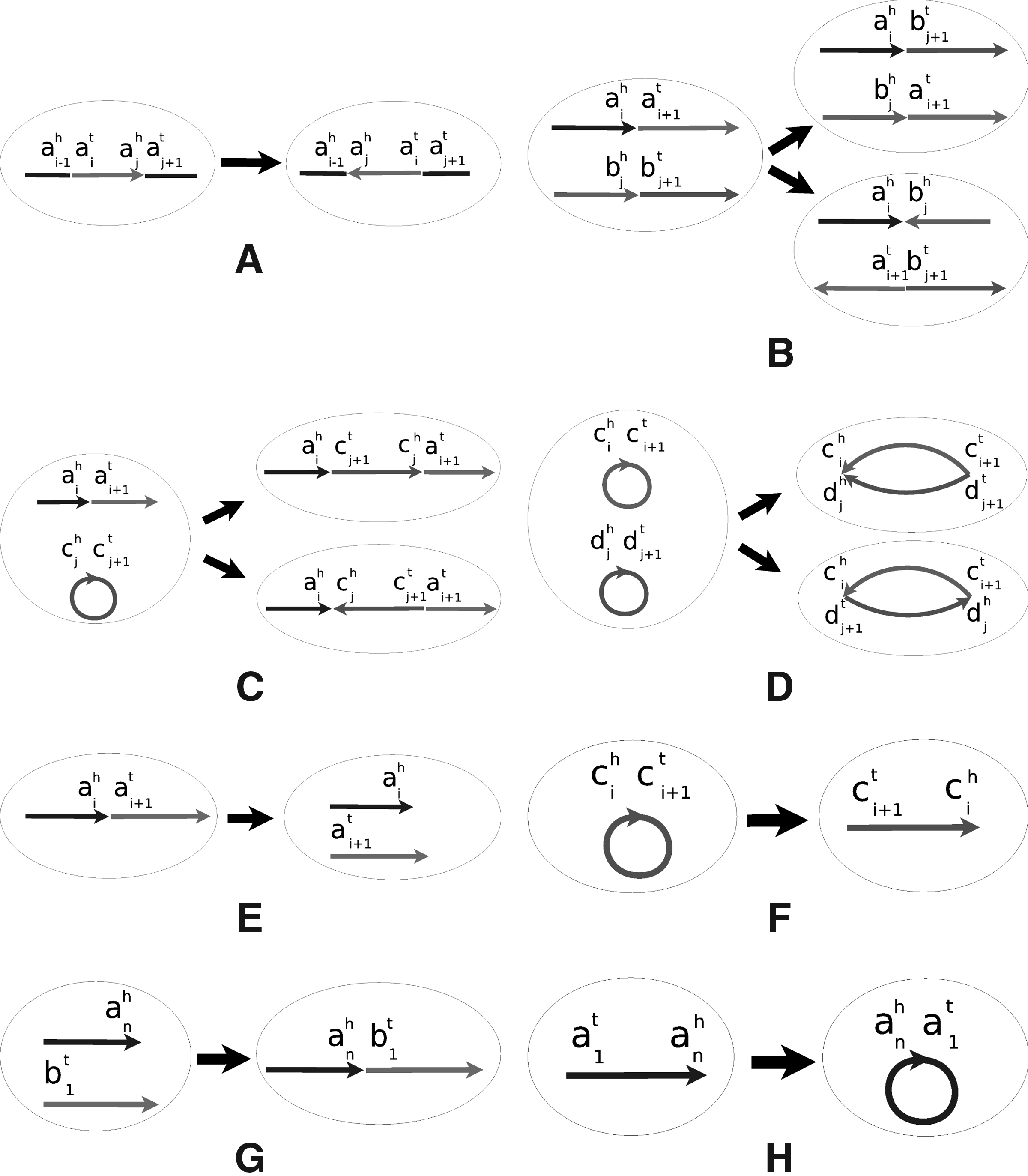
Possible rearrangements.

As mentioned earlier, we do not include a fission that creates a circular intermediate. This choice is based on desired outcomes, not on any notion of mechanism and, in that sense, follows the spirit of the DCJ model itself, since that model's strength is not the verisimilitude of its mechanism, but the simplicity of its formulation and the universality of its set of operations. As we shall see, running our model produces simulated genomes that more closely resemble actual genomes than those produced under a pure DCJ or HP model.

For gene duplication, we uniformly select a position to start duplicating a short segment of chromosomal material and place the new copy to a new position within the genome. We set L_max as the maximum number of genes in the duplicated segment and assume that the number of genes in that segment is a uniform random number between 1 and L_max. For example, select one segment \documentclass{aastex} \usepackage{amsbsy} \usepackage{amsfonts} \usepackage{amssymb} \usepackage{bm} \usepackage{mathrsfs} \usepackage{pifont} \usepackage{stmaryrd} \usepackage{textcomp} \usepackage{portland, xspace} \usepackage{amsmath, amsxtra} \pagestyle{empty} \DeclareMathSizes {10} {9} {7} {6} \begin{document} $$a_{i + 1} \ldots a_{i + L}$$\end{document} to duplicate and insert the copy between one adjacency \documentclass{aastex} \usepackage{amsbsy} \usepackage{amsfonts} \usepackage{amssymb} \usepackage{bm} \usepackage{mathrsfs} \usepackage{pifont} \usepackage{stmaryrd} \usepackage{textcomp} \usepackage{portland, xspace} \usepackage{amsmath, amsxtra} \pagestyle{empty} \DeclareMathSizes {10} {9} {7} {6} \begin{document} $$\{ b_{j}^h , b_{j + 1}^t \}$$\end{document} . Such an operation duplicates L genes and L−1 adjacencies, removes one adjacency, and adds two new adjacencies; thus genes \documentclass{aastex} \usepackage{amsbsy} \usepackage{amsfonts} \usepackage{amssymb} \usepackage{bm} \usepackage{mathrsfs} \usepackage{pifont} \usepackage{stmaryrd} \usepackage{textcomp} \usepackage{portland, xspace} \usepackage{amsmath, amsxtra} \pagestyle{empty} \DeclareMathSizes {10} {9} {7} {6} \begin{document} $$a_{i + 1} , \ldots , a_{i + L - 1}$$\end{document} and a_i+L are added to the multiset of genes, the adjacency \documentclass{aastex} \usepackage{amsbsy} \usepackage{amsfonts} \usepackage{amssymb} \usepackage{bm} \usepackage{mathrsfs} \usepackage{pifont} \usepackage{stmaryrd} \usepackage{textcomp} \usepackage{portland, xspace} \usepackage{amsmath, amsxtra} \pagestyle{empty} \DeclareMathSizes {10} {9} {7} {6} \begin{document} $$\{ b_{j}^h , b_{j + 1}^t \}$$\end{document} is removed, and L + 1 new adjacencies, \documentclass{aastex} \usepackage{amsbsy} \usepackage{amsfonts} \usepackage{amssymb} \usepackage{bm} \usepackage{mathrsfs} \usepackage{pifont} \usepackage{stmaryrd} \usepackage{textcomp} \usepackage{portland, xspace} \usepackage{amsmath, amsxtra} \pagestyle{empty} \DeclareMathSizes {10} {9} {7} {6} \begin{document} $$\{ b_{j}^h , a_{i + 1}^t \}$$\end{document} , \documentclass{aastex} \usepackage{amsbsy} \usepackage{amsfonts} \usepackage{amssymb} \usepackage{bm} \usepackage{mathrsfs} \usepackage{pifont} \usepackage{stmaryrd} \usepackage{textcomp} \usepackage{portland, xspace} \usepackage{amsmath, amsxtra} \pagestyle{empty} \DeclareMathSizes {10} {9} {7} {6} \begin{document} $$\{ a_{i + 1}^h , a_{i + 2}^t \} , \ldots , \{ a_{i + L}^h , b_{j + 1}^t \}$$\end{document} , are added. For gene loss, we uniformly select one gene from the set of all candidate genes and delete it, restricting gene loss to the deletion of a single gene copy at a time, following Lynch (2007). For example, if we delete gene a_i in the chromosome \documentclass{aastex} \usepackage{amsbsy} \usepackage{amsfonts} \usepackage{amssymb} \usepackage{bm} \usepackage{mathrsfs} \usepackage{pifont} \usepackage{stmaryrd} \usepackage{textcomp} \usepackage{portland, xspace} \usepackage{amsmath, amsxtra} \pagestyle{empty} \DeclareMathSizes {10} {9} {7} {6} \begin{document} $$( \ldots a_{i - 1}a_{i}a_{i + 1} \ldots )$$\end{document} , one copy of a_i is removed from the multiset of genes, while two adjacencies, \documentclass{aastex} \usepackage{amsbsy} \usepackage{amsfonts} \usepackage{amssymb} \usepackage{bm} \usepackage{mathrsfs} \usepackage{pifont} \usepackage{stmaryrd} \usepackage{textcomp} \usepackage{portland, xspace} \usepackage{amsmath, amsxtra} \pagestyle{empty} \DeclareMathSizes {10} {9} {7} {6} \begin{document} $$\{ a_{i - 1}^h , a_i^t \}$$\end{document} and \documentclass{aastex} \usepackage{amsbsy} \usepackage{amsfonts} \usepackage{amssymb} \usepackage{bm} \usepackage{mathrsfs} \usepackage{pifont} \usepackage{stmaryrd} \usepackage{textcomp} \usepackage{portland, xspace} \usepackage{amsmath, amsxtra} \pagestyle{empty} \DeclareMathSizes {10} {9} {7} {6} \begin{document} $$\{ a_{i}^h , a_{i + 1}^t \}$$\end{document} , are replaced by one adjacency, \documentclass{aastex} \usepackage{amsbsy} \usepackage{amsfonts} \usepackage{amssymb} \usepackage{bm} \usepackage{mathrsfs} \usepackage{pifont} \usepackage{stmaryrd} \usepackage{textcomp} \usepackage{portland, xspace} \usepackage{amsmath, amsxtra} \pagestyle{empty} \DeclareMathSizes {10} {9} {7} {6} \begin{document} $$\{ a_{i - 1}^h , a_{i + 1}^t \}$$\end{document} .

3. Results

3.1. Model restricted to rearrangements

Edit distance computation

The edit distance between two genomes is the minimum number of allowed evolutionary operations necessary to transform one genome into the other.

Consider two genomes with equal gene content and no duplicate genes. If both genomes consist of only linear chromosomes, the model of Hannenhalli and Pevzner (1995) allows the computation of the edit distance under inversions, translocations, fusions, and fissions, hereafter the HP distance. The edit distance in our model can be no larger than the HP distance, since our model includes all operations in the HP model and more (circularizations and linearizations).

In fact, the two edit distances are equal for genomes composed of only linear chromosomes. Suppose there are intermediate circular chromosomes in some sorting path in our model; then we can always find pairs of operations, one to circularize a linear chromosome and the other to linearize that circular chromosome, that can be replaced by a fission and a fusion in the HP model. So any optimal sorting path in our model can be transformed into an optimal sorting path of equal length in the HP model; therefore, the edit distance in our model is equal to the HP distance—although the number of optimal sorting paths may be different.

If two genomes have both linear and circular chromosomes, the edit distance in our model can be no smaller than the DCJ distance (Bergeron et al., 2006), since the DCJ model includes all operations in our model and more. Bergeron et al. (2009) gave a linear-time algorithm to compute the extra cost of not resorting to “forbidden” DCJ operations to compute the HP distance; their algorithm also applies to our model. Thus, for any two genomes with equal gene content and no duplicate genes, the edit distance in our model can be computed in linear time.

3.2. Genome structure prediction

In this section, we prove that our new model respects the distinction between eukaryotic and prokaryotic genomes. Note that the following theorems do not deal with the process of chromosome evolution, only with its endpoint.

Theorem 1

Let the ancestral genome have one circular chromosome with n genes. After O(n) rearrangements events, with probability 1 − n ^−O(1) , the final genome contains a single circular chromosome or a collection of O(log n) linear chromosomes.

Proof

We examine the effect of rearrangements on the genome structure. Given the original genome with one circular chromosome, only one of our eight cases can result in a linearization: select the same adjacency twice (Fig. 2f). Once we have only linear chromosomes, two cases can directly result in a change in the number of linear or circular chromosomes: select the same adjacency twice (Fig. 2e) and select two telomeres (Fig. 2h). The probability for selecting the same adjacency twice is O(1/n); that for selecting two telomeres is O(t²/n²), where t is the number of telomeres. Every time we select the same adjacency twice, we increase the number of linear chromosomes by 1. Let the indicator variable X_i represent whether or not we select the same adjacency twice at the ith step and write k for the number of evolutionary events. Set \documentclass{aastex} \usepackage{amsbsy} \usepackage{amsfonts} \usepackage{amssymb} \usepackage{bm} \usepackage{mathrsfs} \usepackage{pifont} \usepackage{stmaryrd} \usepackage{textcomp} \usepackage{portland, xspace} \usepackage{amsmath, amsxtra} \pagestyle{empty} \DeclareMathSizes {10} {9} {7} {6} \begin{document} $$X = \sum \nolimits_{i = 1}^k X_i$$\end{document} and let μ be the expectation of X. The Chernoff bound shows \documentclass{aastex} \usepackage{amsbsy} \usepackage{amsfonts} \usepackage{amssymb} \usepackage{bm} \usepackage{mathrsfs} \usepackage{pifont} \usepackage{stmaryrd} \usepackage{textcomp} \usepackage{portland, xspace} \usepackage{amsmath, amsxtra} \pagestyle{empty} \DeclareMathSizes {10} {9} {7} {6} \begin{document} \begin{align*}Pr ( X > ( 1 + \delta ) \mu ) < \left ( e^{ \delta} / ( 1 + \delta ) ^{1 + \delta} \right ) ^{ \mu}\end{align*}\end{document}

In our case, k = O(n), μ = O(1), δ = O(logn), so that we get \documentclass{aastex} \usepackage{amsbsy} \usepackage{amsfonts} \usepackage{amssymb} \usepackage{bm} \usepackage{mathrsfs} \usepackage{pifont} \usepackage{stmaryrd} \usepackage{textcomp} \usepackage{portland, xspace} \usepackage{amsmath, amsxtra} \pagestyle{empty} \DeclareMathSizes {10} {9} {7} {6} \begin{document} \begin{align*}Pr ( X > O ( \log n ) ) < n^{ - O ( 1 ) }\end{align*}\end{document}

Let the indicator variable Y_i represent whether or not we select two telomeres at the ith step. Since t = 2X, t is bounded by O(logn) with probability 1 − n^−O(1). Thus, with probability 1 − n^−O(1), we have \documentclass{aastex} \usepackage{amsbsy} \usepackage{amsfonts} \usepackage{amssymb} \usepackage{bm} \usepackage{mathrsfs} \usepackage{pifont} \usepackage{stmaryrd} \usepackage{textcomp} \usepackage{portland, xspace} \usepackage{amsmath, amsxtra} \pagestyle{empty} \DeclareMathSizes {10} {9} {7} {6} \begin{document} \begin{align*}Pr ( Y_i = 1 ) < O ( ( \log n ) ^2 / n^2 ) ,\end{align*}\end{document}

Now set \documentclass{aastex} \usepackage{amsbsy} \usepackage{amsfonts} \usepackage{amssymb} \usepackage{bm} \usepackage{mathrsfs} \usepackage{pifont} \usepackage{stmaryrd} \usepackage{textcomp} \usepackage{portland, xspace} \usepackage{amsmath, amsxtra} \pagestyle{empty} \DeclareMathSizes {10} {9} {7} {6} \begin{document} $$Y = \sum \nolimits_{i = 1}^k Y_i$$\end{document} . We have \documentclass{aastex} \usepackage{amsbsy} \usepackage{amsfonts} \usepackage{amssymb} \usepackage{bm} \usepackage{mathrsfs} \usepackage{pifont} \usepackage{stmaryrd} \usepackage{textcomp} \usepackage{portland, xspace} \usepackage{amsmath, amsxtra} \pagestyle{empty} \DeclareMathSizes {10} {9} {7} {6} \begin{document} \begin{align*}Pr ( Y > 0 ) \leqslant \sum_{i = 1}^{k}Pr ( Y_i = 1 ) < n^{ - O ( 1 ) }.\end{align*}\end{document}

Overall, then, with probability 1 − n^−O(1), X < O(logn) and Y = 0, which means that the final genome structure has either a collection of O(log n) linear chromosomes or a single circular chromosome. ▪

Theorem 1 tells us that, if the original genomic structure starts from a circular chromosome, most current genomes will contain a single circular chromosome or a collection of linear chromosomes. However, if the initial genome structure was, for example, a mix of linear and circular chromosomes, would such a structure be stable through evolution? We can characterize all stable structures in our model under some mild conditions.

Theorem 2

Let the ancestral genome have n genes and assume that there are positive constants c₁ and α such that each chromosome in the ancestral genome has at least c₁n^α genes. Let c₂ be some constant obeying c₂ > 2c₁. After c₂n^1−αlog n rearrangements, with probability 1 − O(n^−αlog n), the final genome contains either a single circular chromosome or a collection of linear chromosomes.

Proof

In our evolutionary model, consider the case of selecting two adjacencies or one adjacency and one telomere in two different chromosomes. If one of the two chromosomes is circular, a fusion will merge the circular chromosome into the linear chromosome (Fig. 2c). If both chromosomes are circular, a fusion will merge the two chromosomes into a single circular chromosome (Fig. 2d). We use a graph representation, G, for the genome structure, where each circular chromosome is represented by a vertex A_i and all of the linear chromosomes (if any) are represented by a single vertex B. If two adjacencies or one adjacency and one telomere are selected in two different chromosomes, we connect the vertices of these two chromosomes. If we first ignore circularizations of linear chromosomes (Fig. 2h), then the genome ends up with a single circular chromosome or a collection of linear chromosomes if and only if the corresponding final graph G is connected. We therefore bound the probability that the graph G is not connected after c₂n^1−α log n rearrangements. If G is not connected, there is at least one bipartition of the vertices into S₁ and S₂ in which no edge has an endpoint in each subset. Assume there are g₁ and g₂ genes in S₁ and S₂, respectively; then min{g₁, g₂} ≥ c₁n^α and g₁ +g₂ = n. Since there are at most \documentclass{aastex} \usepackage{amsbsy} \usepackage{amsfonts} \usepackage{amssymb} \usepackage{bm} \usepackage{mathrsfs} \usepackage{pifont} \usepackage{stmaryrd} \usepackage{textcomp} \usepackage{portland, xspace} \usepackage{amsmath, amsxtra} \pagestyle{empty} \DeclareMathSizes {10} {9} {7} {6} \begin{document} $$ \frac { 1 } { c_1 } n^ { 1 - \alpha }$$\end{document} chromosomes, we can write \documentclass{aastex} \usepackage{amsbsy} \usepackage{amsfonts} \usepackage{amssymb} \usepackage{bm} \usepackage{mathrsfs} \usepackage{pifont} \usepackage{stmaryrd} \usepackage{textcomp} \usepackage{portland, xspace} \usepackage{amsmath, amsxtra} \pagestyle{empty} \DeclareMathSizes {10} {9} {7} {6} \begin{document} \begin{align*}Pr ( G \ is \ not \ connected ) & < {{{g_1 \choose 2} + {g_2 \choose 2}} \choose {c_2n^{1 - \alpha} \log n}} \Big / {{g_1 + g_2 \choose 2} \choose {c_2n^{1 - \alpha} \log n}} \\ & < ( 1 - c_1 n^{1 - \alpha} ) ^{c_2 n^{1 - \alpha} \log n} < O ( n^{ - 2 \alpha} ) \end{align*}\end{document}

Let indicator variable X_i represent whether or not we select the same adjacency twice at the ith step (Fig. 2e,f) and set \documentclass{aastex} \usepackage{amsbsy} \usepackage{amsfonts} \usepackage{amssymb} \usepackage{bm} \usepackage{mathrsfs} \usepackage{pifont} \usepackage{stmaryrd} \usepackage{textcomp} \usepackage{portland, xspace} \usepackage{amsmath, amsxtra} \pagestyle{empty} \DeclareMathSizes {10} {9} {7} {6} \begin{document} $$X = \sum \nolimits_{i = 1}^{c_2n^{1 - \alpha} \log n}X_i$$\end{document} . We have \documentclass{aastex} \usepackage{amsbsy} \usepackage{amsfonts} \usepackage{amssymb} \usepackage{bm} \usepackage{mathrsfs} \usepackage{pifont} \usepackage{stmaryrd} \usepackage{textcomp} \usepackage{portland, xspace} \usepackage{amsmath, amsxtra} \pagestyle{empty} \DeclareMathSizes {10} {9} {7} {6} \begin{document} \begin{align*}Pr ( X_i = 1 ) & \leqslant 1 / n \\ Pr ( X > 0 ) & \leqslant \sum_{i = 1}^{c_2n^{1 - \alpha} \log n}Pr ( X_i = 1 ) = O ( n^{ - \alpha} \log n ).\end{align*}\end{document}

Now we bound the probability of selecting two telomeres in the same linear chromosome (Fig. 2h), which causes a circularization of this chromosome—the case we deliberately ignored above. For each linear chromosome, there are four possible ways of selecting two corresponding telomeres. Since the number of linear chromosomes l is bounded by \documentclass{aastex} \usepackage{amsbsy} \usepackage{amsfonts} \usepackage{amssymb} \usepackage{bm} \usepackage{mathrsfs} \usepackage{pifont} \usepackage{stmaryrd} \usepackage{textcomp} \usepackage{portland, xspace} \usepackage{amsmath, amsxtra} \pagestyle{empty} \DeclareMathSizes {10} {9} {7} {6} \begin{document} $$ \frac { 1 } { c_1 } n^ { 1 - \alpha }$$\end{document} , there are at most \documentclass{aastex} \usepackage{amsbsy} \usepackage{amsfonts} \usepackage{amssymb} \usepackage{bm} \usepackage{mathrsfs} \usepackage{pifont} \usepackage{stmaryrd} \usepackage{textcomp} \usepackage{portland, xspace} \usepackage{amsmath, amsxtra} \pagestyle{empty} \DeclareMathSizes {10} {9} {7} {6} \begin{document} $$ \frac { 4 } { c_1 } n^ { 1 - \alpha }$$\end{document} ways to circularize one linear chromosome in all (n + l)² ways of selecting two adjacencies or telomeres. Again, let indicator variable Y_i represent circularization of one linear chromosome at the ith step and set \documentclass{aastex} \usepackage{amsbsy} \usepackage{amsfonts} \usepackage{amssymb} \usepackage{bm} \usepackage{mathrsfs} \usepackage{pifont} \usepackage{stmaryrd} \usepackage{textcomp} \usepackage{portland, xspace} \usepackage{amsmath, amsxtra} \pagestyle{empty} \DeclareMathSizes {10} {9} {7} {6} \begin{document} $$Y = \sum \nolimits_{i = 1}^{c_2n^{1 - \alpha} \log n}Y_i$$\end{document} . We have \documentclass{aastex} \usepackage{amsbsy} \usepackage{amsfonts} \usepackage{amssymb} \usepackage{bm} \usepackage{mathrsfs} \usepackage{pifont} \usepackage{stmaryrd} \usepackage{textcomp} \usepackage{portland, xspace} \usepackage{amsmath, amsxtra} \pagestyle{empty} \DeclareMathSizes {10} {9} {7} {6} \begin{document} \begin{align*}Pr ( Y > 0 ) & \leqslant \sum_{i = 1}^{c_2n^{1 - \alpha} \log n}Pr ( Y_i = 1 ) \\ & \leqslant {4c_2 \log n} \big / {c_1n^{2 \alpha}} < O ( n^{ - 2 \alpha} \log n ) \end{align*}\end{document}

Thus, with probability 1 − O(n^−αlog n), we have: G is connected, X = 0, and Y = 0, so that the final genome contains either a single circular chromosome or a collection of linear chromosomes. ▪

The restriction on the minimum size of chromosomes in the ancestral genomes is very mild, since the parameter α can be arbitrarily small.

Our model also predicts, for genomes composed of a collection of linear chromosomes, convergence to a certain number of chromosomes, which depends on the total number of genes.

Theorem 3

Assume there are n genes and fewer than \documentclass{aastex} \usepackage{amsbsy} \usepackage{amsfonts} \usepackage{amssymb} \usepackage{bm} \usepackage{mathrsfs} \usepackage{pifont} \usepackage{stmaryrd} \usepackage{textcomp} \usepackage{portland, xspace} \usepackage{amsmath, amsxtra} \pagestyle{empty} \DeclareMathSizes {10} {9} {7} {6} \begin{document} $$ \frac { 1 + \sqrt { 1 + 4n } } { 2 }$$\end{document} linear chromosomes in the original genome. The number of linear chromosomes increases during rearrangements, converging to \documentclass{aastex} \usepackage{amsbsy} \usepackage{amsfonts} \usepackage{amssymb} \usepackage{bm} \usepackage{mathrsfs} \usepackage{pifont} \usepackage{stmaryrd} \usepackage{textcomp} \usepackage{portland, xspace} \usepackage{amsmath, amsxtra} \pagestyle{empty} \DeclareMathSizes {10} {9} {7} {6} \begin{document} $$ \frac { 1 + \sqrt { 1 + 4n } } { 2 }$$\end{document} .

Proof

Assume there are l linear chromosomes in the original genome. In our model, the number of linear chromosomes increases by 1 with probability \documentclass{aastex} \usepackage{amsbsy} \usepackage{amsfonts} \usepackage{amssymb} \usepackage{bm} \usepackage{mathrsfs} \usepackage{pifont} \usepackage{stmaryrd} \usepackage{textcomp} \usepackage{portland, xspace} \usepackage{amsmath, amsxtra} \pagestyle{empty} \DeclareMathSizes {10} {9} {7} {6} \begin{document} $$ \frac { 1 } { n + l }$$\end{document} and decreases by 1 with probability \documentclass{aastex} \usepackage{amsbsy} \usepackage{amsfonts} \usepackage{amssymb} \usepackage{bm} \usepackage{mathrsfs} \usepackage{pifont} \usepackage{stmaryrd} \usepackage{textcomp} \usepackage{portland, xspace} \usepackage{amsmath, amsxtra} \pagestyle{empty} \DeclareMathSizes {10} {9} {7} {6} \begin{document} $$( \frac { 1 } { n + l } ) ^2$$\end{document} . Since we have \documentclass{aastex} \usepackage{amsbsy} \usepackage{amsfonts} \usepackage{amssymb} \usepackage{bm} \usepackage{mathrsfs} \usepackage{pifont} \usepackage{stmaryrd} \usepackage{textcomp} \usepackage{portland, xspace} \usepackage{amsmath, amsxtra} \pagestyle{empty} \DeclareMathSizes {10} {9} {7} {6} \begin{document} $$l < \frac { 1 + \sqrt { 1 + 4n } } { 2 }$$\end{document} , an increase is more likely. The stable equilibrium follows from the equation \documentclass{aastex} \usepackage{amsbsy} \usepackage{amsfonts} \usepackage{amssymb} \usepackage{bm} \usepackage{mathrsfs} \usepackage{pifont} \usepackage{stmaryrd} \usepackage{textcomp} \usepackage{portland, xspace} \usepackage{amsmath, amsxtra} \pagestyle{empty} \DeclareMathSizes {10} {9} {7} {6} \begin{document} $$ \frac { 1 } { n + l } = ( \frac { l } { n + l } ) ^2$$\end{document} . ▪

These theorems are not affected by duplications and losses, as long as the latter are reflected in the sizes of chromosomes and the total number of genes.

3.3. Sizes of gene families

Of most concern in a duplication and loss model is the distribution of the sizes of the gene families, since that is one of the few aspects of the process that has been observed to obey general laws. Our sole aim in this section is to demonstrate through simulations that our model, which uses the duplication/loss model of Lynch, yields distributions consistent with what Lynch (2007) suggested.

Our experiments start with a genome with no duplicated genes. This genome is then subjected to a prescribed number k, varying from from 0 to 10 times the number of genes, of evolutionary events chosen according to p_d and p_l to obtain different genomes G^k. We test a large number of different choices of parameters on varying sizes of genomes; as the results are consistent throughout, we report two cases: (a) 1,000 genes with L = 10, p_d = 0.2, and p_l = 0.8; and (b) 10,000 genes with L = 10, p_d = 0.4, and p_l = 0.6. The data in Figure 3 summarizes 1,000 runs for each parameter setting. (The parameters chosen correspond to those used in our distance estimation model [Lin et al., 2010].) The shape of the distributions of gene family sizes is generally similar to the observations presented by Lynch (2007).

FIG. 3.

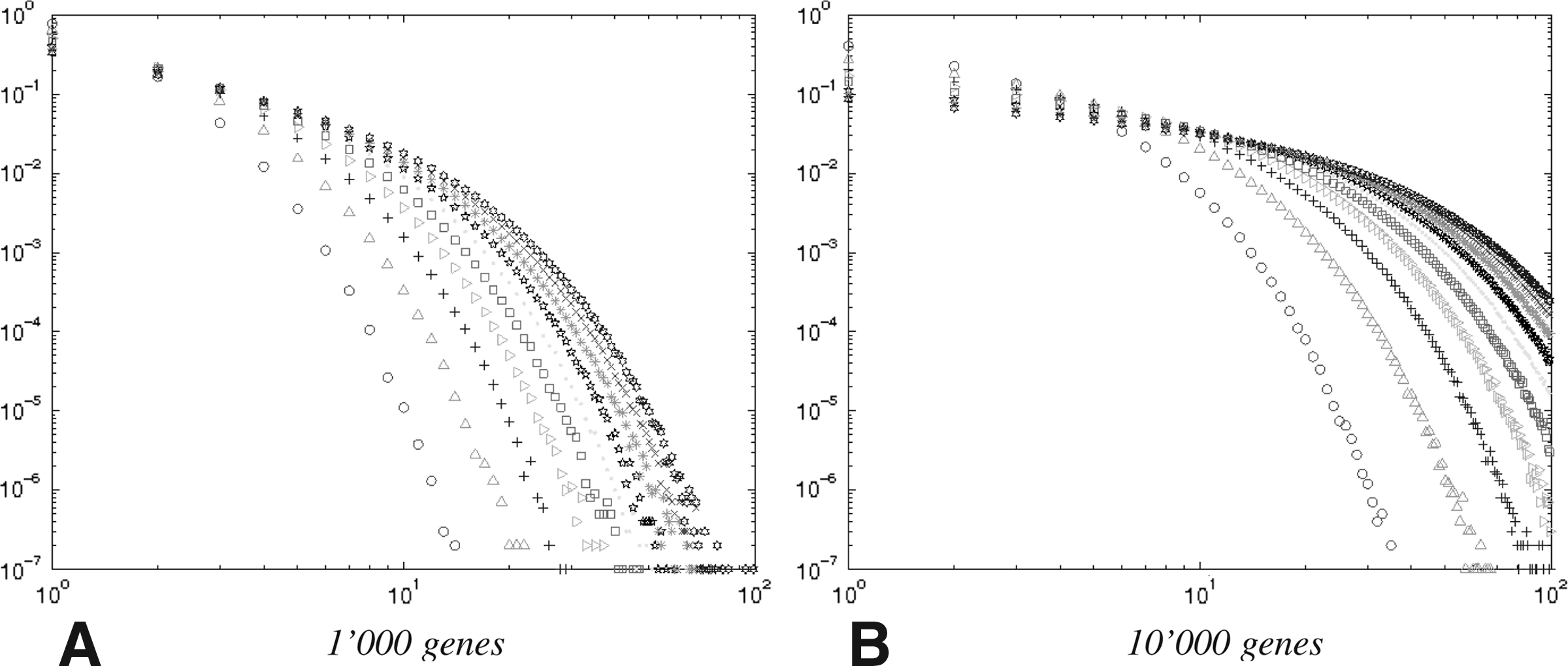
Probability distribution of the size of gene families, for various numbers of events, increasing from the leftmost (#events = #genes) to the rightmost (#events = 10 × #genes).

4. Conclusion

While the mechanism of genome evolution remains unclear, one can nevertheless study different models through simulation and through application to real genomes. Thus, while we make no claims of biological verisimilitude for the operations and constraints within our model, our Theorems 1 and 2 show that our model respects the distinction between the organization of most prokaryotic genomes (one circular chromosome) and that of most eukaryotic genomes (multiple linear chromosomes). In contrast, the HP model (Hannenhalli and Pevzner, 1995) deals with only linear chromosomes, while the DCJ model (Bergeron et al., 2006; Yancopoulos et al., 2005) (assuming uniform distribution of all possible DCJ operations) predicts that over half of modern genomes consisting of only circular chromosomes will have more than one circular chromosome. It is perhaps surprising that a simple modification to the DCJ model (forbidding the least realistic operation) can result in simulated genomes that closely resemble actual genomes—we view this finding as reinforcing the importance of the DCJ model as a basis for future model refinements.

There is evidence about the linearization of circular chromosomes during bacterial evolution (Volff and Altenbuchner, 2000) and the increase in the number of chromosomes of eukaryotic groups by centric fission (Imai, 1978; Imai and Crozier, 1980), both of which accord with Theorem 3. It is interesting to point out that Imai et al. (1986) applied their minimum interaction theory to the genome evolution in eukaryotes to explain the increment in the number of linear chromosomes. Their theory predicts that the highest number of chromosomes in mammals should be 166, while their simulations yield a range of 133–138 for this number (Imai et al., 2002). Despite the fact that both models are based on different sets of oversimplified or unrealistic assumptions, the latter range derived by Imai et al. is similar to the predictions in our model (as well as the models in Hannenhalli and Pevzner [1995], Bergeron et al. [2006], and Yancopoulos et al. [2005], if we assume that the two cuts are uniformly selected) if the number of genes is around 20,000, a fairly typical value for mammals.

Figure 3 shows that our model of gene duplications and losses readily generates distributional forms close to the observations presented by Lynch (2007). Different parameters for gene duplications and losses, and the number of evolutionary events, influence the the distributions of gene family sizes: such information can help us improve the estimation of the actual number of evolutionary events as well as infer the parameters for duplications and losses in our model (Lin et al., 2010).

According to the analytical results in our model, increasing numbers of rearrangements, gene duplications, and gene losses will linearize circular chromosomes, increase the number of linear chromosomes, and increase the number of genes—i.e., will favor a shift from a prokaryotic architecture to a eukaryotic one. However prokaryotic architectures exist in large numbers today—larger by far than eukaryotic ones. The reason is to be found in population sizes. In a large population, as with most prokaryotic organisms, most alleles are likely to be eliminated by purifying selection, whereas, in a small population, neutral or even deleterious mutations can be fixated more easily. Population sizes decreased dramatically in the transition from prokaryotes to multicellular eukaryotes (Lynch, 2007). Thus, many forms of mutant alleles that are able to drift to fixation in multicellular eukaryotes are eliminated by purifying selection in prokaryotes. In a similar way, the fixation of rearrangements, gene duplications, and gene losses (all “rare genomic events” [Rokas and Holland, 2000]) in prokaryotic species is also more difficult compared to that in eukaryotes. Thus, in our model, prokaryotes tend to have one circular chromosome and a small number of genes, while eukaryotes tend to have multiple linear chromosomes and a large number of genes, in response to a reduction in purifying selection. Our model of gene rearrangement, duplication, and loss is the first to give rise naturally to such a structure; and it does so independently of the choice of parameters, which influence only the tapering rate of the size of gene families.

Footnotes

1

Selecting one telomere twice is assimilated to selecting both telomeres of the linear chromosome.

References

Bader

, Moret

, Yan

2001. A fast linear-time algorithm for inversion distance with an experimental comparison. J. Comput. Biol., 8:483–491.

Bergeron

, Mixtacki

, Stoye

2006. A unifying view of genome rearrangements. Lect. Notes Comput. Sci, 4175:163–173.

Bergeron

, Mixtacki

, Stoye

2009. A new linear time algorithm to compute the genomic distance via the double cut and join distance. Theor. Comput. Sci., 410:5300–5316.

Bergeron

, Medvedev

, Stoye

2010. Rearrangement models and single-cut operations. J. Comput. Biol., 17:1213–1225.

Fertin

, Labarre

, Rusu

et al. 2009. Combinatorics of Genome Rearrangements. MIT Press: Cambridge, MA.

Hahn

, Bie

T.D.

, Stajich

et al. 2005. Estimating the tempo and mode of gene family evolution from comparative genomic data. Genome Res., 15:1153–1160.

Hannenhalli

, Pevzner

1995. Transforming mice into men (polynomial algorithm for genomic distance problems) Proc. FOCS’95, 581–592.

Huynen

, van Nimwegen

1998. The frequency distribution of gene family sizes in complete genomes. Mol. Biol. Evol., 15:583–589.

Imai

1978. On the origin of telocentric chromosomes in mammals. J. Theor. Biol., 71:619–637.

10.

Imai

, Crozier

1980. Quantitative analysis of directionality in mammalian karyotype evolution. Am. Naturalist, 116:537–569.

11.

Imai

, Maruyama

, Gojobori

et al. 1986. Theoretical bases for karyotype evolution. 1. The minimum-interaction hypothesis. Am. Naturalist, 128:900–920.

12.

Imai

, Satta

, Wada

et al. 2002. Estimation of the highest chromosome number of eukaryotes based on the minimum interaction theory. J. Theor. Biol., 217:61–74.

13.

Koonin

, Wolf

, Karev

2002. The structure of the protein universe and genome evolution. Nature, 420:218–223.

14.

Lin

, Rajan

, Swenson

et al. 2010. Estimating true evolutionary distances under rearrangements, duplications, and losses. Proc. 8th Asia Pac. Bioinform. Conf. (APBC’10) To appear in BMC Bioinformatics, 11,Suppl. 1:S54.

15.

Luscombe

, Qian

, Zhang

et al. 2002. The dominance of the population by a selected few: power-law behaviour applies to a wide variety of genomic properties. Genome Biol., 3:8.

16.

Lynch

2007. The Origins of Genome Architecture. Sinauer: Sunderland, MA.

17.

Qian

, Luscombe

, Gerstein

2001. Protein family and fold occurrence in genomes: power-law behavior and evolutionary model. J. Mol. Biol., 313:673–681.

18.

Rokas

, Holland

2000. Rare genomic changes as a tool for phylogenetics. Trends Ecol. Evol., 15:454–459.

19.

Sturtevant

1921. A case of rearrangement of genes in Drosophila. Proc. Natl. Acad. Sci. USA, 7:235–237.

20.

Sturtevant

, Dobzhansky

1936. Inversions in the third chromosome of wild races of Drosophila pseudoobscura, and their use in the study of the history of the species. Proc. Natl. Acad. Sci. USA, 22:448–450.

21.

Volff

J.-N.

, Altenbuchner

2000. A new beginning with new ends: linearisation of circular chromosomes during bacterial evolution. FEMS Microbiol. Lett., 186:143–150.

22.

Yanai

, Camacho

, DeLisi

2000. Predictions of gene family distributions in microbial genomes: evolution by gene duplication and modification. Phys. Rev. Lett., 85:2641–2644.

23.

Yancopoulos

, Attie

, Friedberg

2005. Efficient sorting of genomic permutations by translocation, inversion and block interchange. Bioinformatics, 21:3340–3346.