Constructing Logical Models of Gene Regulatory Networks by Integrating Transcription Factor–DNA Interactions with Expression Data: An Entropy-Based Approach

Abstract

Models of gene regulatory networks (GRNs) attempt to explain the complex processes that determine cells' behavior, such as differentiation, metabolism, and the cell cycle. The advent of high-throughput data generation technologies has allowed researchers to fit theoretical models to experimental data on gene-expression profiles. GRNs are often represented using logical models. These models require that real-valued measurements be converted to discrete levels, such as on/off, but the discretization often introduces inconsistencies into the data. Dimitrova et al. posed the problem of efficiently finding a parsimonious resolution of the introduced inconsistencies. We show that reconstruction of a logical GRN that minimizes the errors is NP-complete, so that an efficient exact algorithm for the problem is not likely to exist. We present a probabilistic formulation of the problem that circumvents discretization of expression data. We phrase the problem of error reduction as a minimum entropy problem, develop a heuristic algorithm for it, and evaluate its performance on mouse embryonic stem cell data. The constructed model displays high consistency with prior biological knowledge. Despite the oversimplification of a discrete model, we show that it is superior to raw experimental measurements and demonstrates a highly significant level of identical regulatory logic among co-regulated genes. A software implementing the method is freely available at: http://acgt.cs.tau.ac.il/modent

1. Introduction

Gene regulatory networks (GRNs) play an important role in orchestrating the complex processes of life. An understanding of these networks and their behavior can elucidate complex processes of disease progression. The logical modeling approach describes a GRN and its dynamics as a set of entities that take discrete levels (e.g., active/inactive). Each entity's level is a function of the levels of certain other entities. Models can assume synchronous or asynchronous updates. The first logical models in biology were presented in the 1970s by Kauffman, Thomas, and colleagues (Glass and Kauffman, 1973; Thomas, 1973). For a review on logical models, see Karlebach and Shamir (2008). In recent years, mapping between logical values and continuous measurements has been revisited and empowered by high-throughput experimental data.

Akutsu et al. (1999) proposed a polynomial algorithm that infers regulatory interactions from experimental data by finding for each gene a Boolean function that predicts its level with maximal accuracy. The inputs of that function are the levels of the gene's regulators. This algorithm requires that continuous expression data first be discretized into Boolean values (i.e., that each real value will be converted into a Boolean one), and then it selects the function and regulators that are in best agreement with the discretized data. A later extension allows each discretized sample to be associated with a continuous confidence value (Lähdesmäki et al., 2003), namely the reliability of each microarray profile (a vector of gene expression values) in the dataset. Akutsu et al. (2009) also studied the case in which only partial experimental data are available, and showed that learning the regulation functions in this setting is NP-complete.

Segal et al. (2003) developed a methodology that uses expression data for inferring regulatory functions formulated as decision trees: each node of the tree corresponds to a regulator, and the level of the regulatee is determined by traversing the tree from root to leaf, selecting a child at each node by comparing the regulator's continuous expression level to some threshold value. The algorithm of Segal et al. (2003) clusters genes into groups that have a similar expression pattern and assigns to every cluster its set of regulators.

Shamir and Tanay presented an efficient algorithm that assumes a monotone relationship between a transcription factor's (TF) continuous level, its affinity to a target gene and the strength of regulation, and uses this assumption to determine whether or not a target gene is activated. Since their algorithm requires TF-target affinities, they also suggested a method for inferring the affinity of a TF to its target genes (Shamir and Tanay, 2003).

The logical rules that govern gene expression were also studied for specific systems. Cox et al. (Cox, et al, 2007) created ∼300 artificial Escherichia coli promoters and analyzed their regulatory logic and other properties, using population-level expression data. The promoters were composed from target sites of two activators and two repressors. The authors observed that basal activity level and strength of induction for genes regulated by a single activator are not correlated. This shows that naive discretization of expression data is likely to produce mistakes.

It should be noted here that inferring discrete logic from continuous measurements depends on the activity threshold of the regulated gene; for example, in a Boolean model, the output should be 1 when the regulated gene's product is present in a sufficient amount to perform its role in the model, such as activating another gene. Thus, the threshold may be specific to the regulated gene. In addition, the closer a real expression value is to the threshold, the greater the chance that the mapping to a discrete value is incorrect.

Tsong et al. (2006) identified mating genes that were negatively regulated in Saccharomyces cerevisiae and positively regulated in an ancestral specie. They showed that the change in logic occurred in two steps: first, expression became independent of an activator, and second, then it came under the influence of a repressor. The changes occurred due to mutations in regulatory sequences, suggesting that changes in regulatory logic may have played a major role in modifying organism fitness during evolution.

Mayo et al. (2006) mutated regulatory sequences in the lac operon of E. coli and showed that certain mutations can change the logic. They also found that the logic is plastic (i.e., many mutations do not cancel a regulation but rather change its logic). This finding further supports the notion that changes in regulatory logic may have played an important role in evolution.

In this study, we show that given a model and discretized expression data that contain errors, the problem of correcting these errors using a minimal number of changes is computationally hard. This resolves an open problem stated in Dimitrova et al. (2010). In the next section, Section 2, we reformulate the problem probabilistically, and present an algorithm for constructing a Boolean model from partial prior knowledge and real-valued expression data aimed at providing a practical solution to the problem. In Section 3, we demonstrate the effectiveness of the method by using the algorithm to construct a logical model of the mouse embryonic stem cell network, and make some observations about the properties of the inferred network.

A software called ModEnt implementing the method is freely available at: http://acgt.cs.tau.ac.il/modent

2. Methods

In a Boolean network model of a GRN, every gene is associated with an entity that can take the levels 0 and 1, which correspond to the inactive and active states of the gene, respectively. Gene regulation is described by assigning a Boolean function to each gene: the levels of a gene's regulators are the inputs of that gene's regulation function, and the effect of the regulator levels on the target gene's level is the output of the function. The model is synchronous: If time-series data are available, the levels of the regulators of each gene at time t-1 determine its level at time t according to its specific regulation logic. More formally, if \documentclass{aastex} \usepackage{amsbsy} \usepackage{amsfonts} \usepackage{amssymb} \usepackage{bm} \usepackage{mathrsfs} \usepackage{pifont} \usepackage{stmaryrd} \usepackage{textcomp} \usepackage{portland, xspace} \usepackage{amsmath, amsxtra} \pagestyle{empty} \DeclareMathSizes {10} {9} {7} {6} \begin{document} $$e_{ ( 1 ) }^t , \ldots , e_{ ( K ) }^t$$\end{document} are the (discretized) levels of the entities at time t, and if \documentclass{aastex} \usepackage{amsbsy} \usepackage{amsfonts} \usepackage{amssymb} \usepackage{bm} \usepackage{mathrsfs} \usepackage{pifont} \usepackage{stmaryrd} \usepackage{textcomp} \usepackage{portland, xspace} \usepackage{amsmath, amsxtra} \pagestyle{empty} \DeclareMathSizes {10} {9} {7} {6} \begin{document} $$r_1^i , \ldots , r_{n_i}^i$$\end{document} are the regulators of entity i and the regulatory logic is f, then \documentclass{aastex} \usepackage{amsbsy} \usepackage{amsfonts} \usepackage{amssymb} \usepackage{bm} \usepackage{mathrsfs} \usepackage{pifont} \usepackage{stmaryrd} \usepackage{textcomp} \usepackage{portland, xspace} \usepackage{amsmath, amsxtra} \pagestyle{empty} \DeclareMathSizes {10} {9} {7} {6} \begin{document} $$f ( e_{ ( r_1^{\,i} ) }^{t - 1} , e_{ ( r_2^{\,i} ) }^{t - 1} , \ldots , e_{ ( r_{n_i}^i ) }^{t - 1} ) = e_{ ( i ) }^t$$\end{document} for every i, t. If such data are not available, or if the time intervals between measurements are relatively long, a steady state can be assumed, in which case the regulation function produces an output at time t that agrees with its inputs at the same time t. For the sake of discussion, let us assume from now on that the data are steady state, though the same method applies to time-series data.

Comparison of a given model to discretized expression data may reveal discrepancies. A discrepancy occurs when the same inputs of a regulation function produce more than one output. For example, if a gene has two regulators that take level 0 in two profiles, but the gene itself has level 0 in one experiment and level 1 in the other, a discrepancy occurs. The source of the discrepancy can be noise or wrong assignment of discrete value to the target gene or to one of the regulators. Dimitrova et al. (2010) state the need for systematic handling of discrepancies as an open problem. When there are multiple discrepancies, we seek here the simplest explanation—the one that requires a minimal number of changes to the profiles of both the regulators and regulatees. We next show that this problem is NP-hard.

Theorem

Given the topology of a Boolean network model and binary expression profiles of the network's genes, resolving the discrepancies with a minimum number of changes is NP-hard.

Proof

We will show a reduction from the NP-complete problem Vertex Cover (Karp, 1972) to the decision problem: Given a GRN, a set of discretized microarray profiles and a number k, can all the discrepancies be resolved by at most k changes to the profiles?

Let (G(V, E), k) be the input for the Vertex Cover problem, where G(V,E) is an undirected graph and k is an integer between 1 and |V|. Construct a GRN as follows: For every vertex v in V, add a gene entity v to the GRN. For every edge e = (u,v) in E, define a new gene e_uv and identify the genes that correspond to u and v as the common regulators of e_uv (the regulatee). Figure 1a illustrates this construction. Hence, the original vertices are regulators (and are not regulated), and the new vertices correspond to regulatees. The set of microarray experiments will contain two profiles. In the first the levels of all the genes will be 0. In the second, the levels of all the regulators will be 0 and the levels of all the regulatee genes will be 1 (Fig. 1b). Since the levels of the regulators are the same in both profiles, and the levels of the regulatees are not, there are discrepancies. Clearly, this reduction can be performed in polynomial time.

FIG. 1.
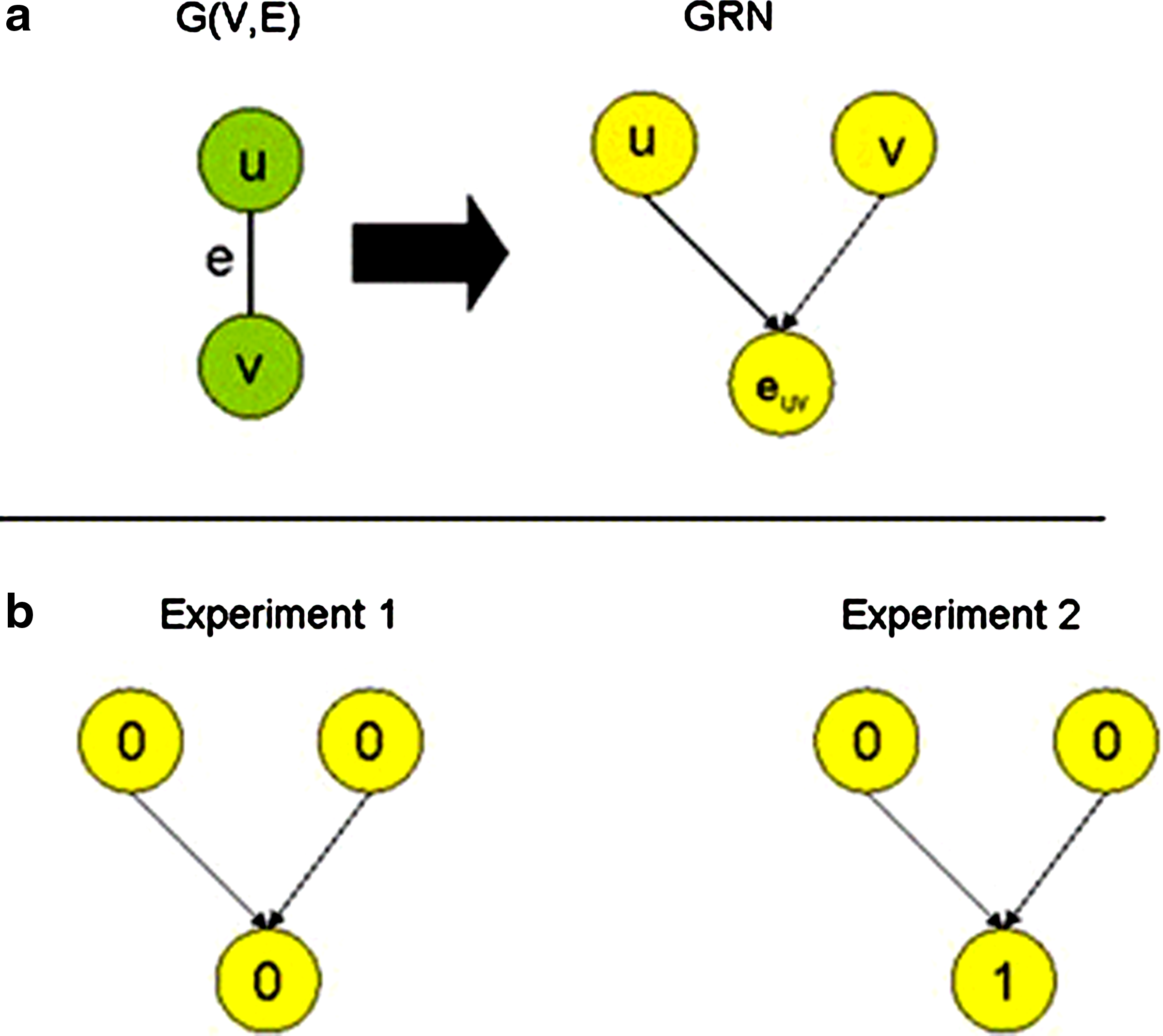
Reduction from Vertex Cover to resolution of discrepancies in microarray expression data with respect to a gene regulatory network (GRN). (a) The graph that is the input for Vertex Cover is shown in green, and the resulting GRN is shown in yellow. (b) The Boolean values of every entity in the two microarray experiments.

Suppose there is a vertex cover S of size at most k. For every vertex u that belongs to S, change the level of the corresponding gene in the second experiment to 1. Since every regulatee corresponds to an edge in G, and its regulators are vertices that are adjacent to that edge, for every regulatee at least one of its regulators changes in experiment 2. Therefore, all the discrepancies are resolved by at most k changes.

Now, assume conversely that there are k changes that resolve all discrepancies. If after the changes there is a regulatee that has the same level in the two profiles (i.e., its level was changed by the solution) and each of its regulators has the same level in the two profiles, we will restore that regulatee's level to 0 in profile 1 and 1 in profile 2, and change the level of one of its regulators in profile 1. This does not increase the total number of changes: The regulatee has regained the levels it had before any changes took place, which cancels at least one change, and a single change was made to a regulator's level. We repeat this for every regulatee that changes its levels from the original levels assigned by the reduction, and thus obtain a set of at most k changes—all of which are in regulator levels—with no discrepancies. Now define a set S that contains the nodes corresponding to every regulator that has different values in the two profiles. This set is of size at most k. For every edge in G, there is a vertex in S that is adjacent to it, because every regulatee has at least one regulator that has different levels in the two experiments. Therefore, S is a vertex cover.

It remains to show that the problem is in NP. Given k changes, we perform them and check in polynomial time whether there are any discrepancies left. ▪

We now approach the problem from a different direction: we return to the real-valued expression profiles, and instead of discretizing them, a process that may cause discrepancies that are difficult to resolve, we take a probabilistic approach. We interpret the real-valued profiles probabilistically, select a set of TF-target interactions that minimizes the total entropy, and use the selected topology and the probabilistically-interpreted profiles to resolve discrepancies. Our algorithm is outlined in Figure 2.

FIG. 2.
An outline of our algorithm. The input consists of real valued expression profiles (a) and a set of putative regulations of genes by transcription factors (b). The expression profiles are interpreted probabilistically (c) and used for determining the topology of the network by selecting a set of regulators that minimize the entropy (d). In this process, some putative interactions are rejected (dashed arrows), and some new interactions are added (red arrows). The network's regulation functions (e) are determined using the probabilistically interpreted expression profiles and the inferred topology.

Following is a detailed description of the algorithm. We interpret a vector of continuous values as a probability distribution over all possible Boolean vectors of the same dimension. In other words, instead of creating a single Boolean vector with probability 1 for a given continuous vector, we create all possible Boolean vectors of the same dimension, and assign each such vector a probability. The probabilities are chosen as follows: First, normalize the continuous expression values of every gene to have mean 0 and standard deviation 1.5 (a value determined empirically). Second, after normalization, set the probability that a single (one-dimensional) real value c corresponds to the Boolean value 1 to \documentclass{aastex} \usepackage{amsbsy} \usepackage{amsfonts} \usepackage{amssymb} \usepackage{bm} \usepackage{mathrsfs} \usepackage{pifont} \usepackage{stmaryrd} \usepackage{textcomp} \usepackage{portland, xspace} \usepackage{amsmath, amsxtra} \pagestyle{empty} \DeclareMathSizes {10} {9} {7} {6} \begin{document} $$\lambda ( c ) = \frac { 1 } { 1 + e^ { - c } } $$\end{document} (the logistic function with parameter value c). The probability that a real-valued vector \documentclass{aastex} \usepackage{amsbsy} \usepackage{amsfonts} \usepackage{amssymb} \usepackage{bm} \usepackage{mathrsfs} \usepackage{pifont} \usepackage{stmaryrd} \usepackage{textcomp} \usepackage{portland, xspace} \usepackage{amsmath, amsxtra} \pagestyle{empty} \DeclareMathSizes {10} {9} {7} {6} \begin{document} $$\overline{c}$$\end{document} corresponds to a specific Boolean vector \documentclass{aastex} \usepackage{amsbsy} \usepackage{amsfonts} \usepackage{amssymb} \usepackage{bm} \usepackage{mathrsfs} \usepackage{pifont} \usepackage{stmaryrd} \usepackage{textcomp} \usepackage{portland, xspace} \usepackage{amsmath, amsxtra} \pagestyle{empty} \DeclareMathSizes {10} {9} {7} {6} \begin{document} $$\overline{b}$$\end{document} then becomes \documentclass{aastex} \usepackage{amsbsy} \usepackage{amsfonts} \usepackage{amssymb} \usepackage{bm} \usepackage{mathrsfs} \usepackage{pifont} \usepackage{stmaryrd} \usepackage{textcomp} \usepackage{portland, xspace} \usepackage{amsmath, amsxtra} \pagestyle{empty} \DeclareMathSizes {10} {9} {7} {6} \begin{document} \begin{align} p ({\overline b} \ \mid \ {\overline c}) = \prod_{i \mid b_i = 1} \frac {1} {1 + e^{- c_i}} \prod_{i \mid b_i = 0} \left( 1 - \frac {1} {1 + e^{- c_i}} \right), \end{align} \end{document}

where c_i (b_i) is the value of the i^th entry of \documentclass{aastex} \usepackage{amsbsy} \usepackage{amsfonts} \usepackage{amssymb} \usepackage{bm} \usepackage{mathrsfs} \usepackage{pifont} \usepackage{stmaryrd} \usepackage{textcomp} \usepackage{portland, xspace} \usepackage{amsmath, amsxtra} \pagestyle{empty} \DeclareMathSizes {10} {9} {7} {6} \begin{document} $$\overline{c}$$\end{document} ( \documentclass{aastex} \usepackage{amsbsy} \usepackage{amsfonts} \usepackage{amssymb} \usepackage{bm} \usepackage{mathrsfs} \usepackage{pifont} \usepackage{stmaryrd} \usepackage{textcomp} \usepackage{portland, xspace} \usepackage{amsmath, amsxtra} \pagestyle{empty} \DeclareMathSizes {10} {9} {7} {6} \begin{document} $$\overline{b}$$\end{document} ). Note that by setting the standard deviation value for all the genes one avoids using any parameters in the logistic function.

Given a continuous dataset of n i.i.d. profiles, the probability of seeing the Boolean vector \documentclass{aastex} \usepackage{amsbsy} \usepackage{amsfonts} \usepackage{amssymb} \usepackage{bm} \usepackage{mathrsfs} \usepackage{pifont} \usepackage{stmaryrd} \usepackage{textcomp} \usepackage{portland, xspace} \usepackage{amsmath, amsxtra} \pagestyle{empty} \DeclareMathSizes {10} {9} {7} {6} \begin{document} $$\overline{b}$$\end{document} in this dataset is: \documentclass{aastex} \usepackage{amsbsy} \usepackage{amsfonts} \usepackage{amssymb} \usepackage{bm} \usepackage{mathrsfs} \usepackage{pifont} \usepackage{stmaryrd} \usepackage{textcomp} \usepackage{portland, xspace} \usepackage{amsmath, amsxtra} \pagestyle{empty} \DeclareMathSizes {10} {9} {7} {6} \begin{document} \begin{align} P ({\overline b}) = \frac {1} {n} \sum_{{\overline c}^{\,j} \in profiles} p ({\overline b} \ \mid \ {\overline c}^{\,j}) \tag{} \end{align} \end{document}

In other words, for each Boolean vector, the probabilities that each continuous vector corresponds to it are averaged. In practice, the samples may not be i.i.d, but that assumption is made for the sake of this analysis.

With the probability distribution over all Boolean vectors at hand, information theory can be used to evaluate different topologies of the network. Suppose we know which of the genes are transcription factors (TFs) and assume that all regulators are TFs. Denote by H^C(x|Y_x) the conditional entropy for a gene x and a set Y_x of regulators as computed using continuous data. We use this notation in order to stress that the conditional entropy is a function of continuous values—a fact that will be used by our algorithm. Select for every gene x the set Y_x of regulators that gives the best H^C(x|Y_x) score among all sets of TFs.

Since in practice a larger set of regulators will tend to score better than a smaller one, a threshold that will separate significant improvement from insignificant improvement is needed: when increasing the set of regulators, any improvement less than the threshold will be considered insignificant. This threshold can be estimated empirically by computing the average and standard deviation of the improvement in entropy that occurs when non-regulator genes are assigned as regulators. Improvement that surpasses the average by 3 standard deviations will be interpreted as non-random. We refer to this threshold value as τ.

After the network structure is constructed, steepest descent can be used for decreasing the entropy: given the set Y_x minimizing the score H^C(x|Y_x) for every gene x, perform steepest descent on the score \documentclass{aastex} \usepackage{amsbsy} \usepackage{amsfonts} \usepackage{amssymb} \usepackage{bm} \usepackage{mathrsfs} \usepackage{pifont} \usepackage{stmaryrd} \usepackage{textcomp} \usepackage{portland, xspace} \usepackage{amsmath, amsxtra} \pagestyle{empty} \DeclareMathSizes {10} {9} {7} {6} \begin{document} $$\sum_{x \in genes} { H}^{C} ( {x} \mid {Y_x} )$$\end{document} , i.e. on the total entropy of the network. We compute the derivative of the total entropy function with respect to each gene and regulator and change their profiles in the direction of the gradient, and repeat this iteratively until the change in entropy is very small.

If we had discrete profiles and change a level from 0 to 1, the value of the conditional entropy will also change. Since we do not discretize, we have continuous profiles, and every function H^C(x|Y_x) is a function of continuous values. Therefore, H^C(x|Y_x) will change with every change of one of its continuous parameters. Given the real level c_ij of gene i at profile j, the partial derivative of the total entropy with respect to c_ij can be computed exactly. By the chain rule for conditional entropy, we have: \documentclass{aastex} \usepackage{amsbsy} \usepackage{amsfonts} \usepackage{amssymb} \usepackage{bm} \usepackage{mathrsfs} \usepackage{pifont} \usepackage{stmaryrd} \usepackage{textcomp} \usepackage{portland, xspace} \usepackage{amsmath, amsxtra} \pagestyle{empty} \DeclareMathSizes {10} {9} {7} {6} \begin{document} \begin{align} \frac {\partial} {\partial c_{ij}} H^C (x \mid Y_x) = \frac {\partial} {\partial c_{ij}} H^C (x , Y_x) - \frac {\partial} {\partial c_{ij}} H^C (Y_x) \end{align} \end{document}

We show how to compute H^C(Y_x). The computation of H^C(x,Y_x) only differs in indices and is omitted: \documentclass{aastex} \usepackage{amsbsy} \usepackage{amsfonts} \usepackage{amssymb} \usepackage{bm} \usepackage{mathrsfs} \usepackage{pifont} \usepackage{stmaryrd} \usepackage{textcomp} \usepackage{portland, xspace} \usepackage{amsmath, amsxtra} \pagestyle{empty} \DeclareMathSizes {10} {9} {7} {6} \begin{document} \begin{align} & \frac {\partial} {\partial c_{ij}} H^C (Y_x) = \frac {\partial} {\partial c_{ij}} \sum_{Y_x} P (Y_x) \log P (Y_x) = \\ & = - \sum_{Y_x} \bigg[ \frac {\partial} {\partial c_{ij}} P (Y_x) \bigg] \log P (Y_x) - \sum_Y P (Y_x) \bigg[ \frac {\partial} {\partial c_{ij}} \log P (Y_x) \bigg] = \\ & = - \sum_{Y_x} \bigg[ \frac {\partial} {\partial c_{ij}} P (Y_x) \bigg] \log P (Y_x) - \sum_Y \frac {\partial} {\partial c_{ij}} P (Y_x) \end{align} \end{document}

where the sum is over all Boolean values of the vector Y_x. The probability of a specific Boolean value of the vector Y_x is given by (), and for \documentclass{aastex} \usepackage{amsbsy} \usepackage{amsfonts} \usepackage{amssymb} \usepackage{bm} \usepackage{mathrsfs} \usepackage{pifont} \usepackage{stmaryrd} \usepackage{textcomp} \usepackage{portland, xspace} \usepackage{amsmath, amsxtra} \pagestyle{empty} \DeclareMathSizes {10} {9} {7} {6} \begin{document} $$ \frac { \partial P ( Y_x ) } { \partial c_ { ij } } $$\end{document} , we have the following sum: \documentclass{aastex} \usepackage{amsbsy} \usepackage{amsfonts} \usepackage{amssymb} \usepackage{bm} \usepackage{mathrsfs} \usepackage{pifont} \usepackage{stmaryrd} \usepackage{textcomp} \usepackage{portland, xspace} \usepackage{amsmath, amsxtra} \pagestyle{empty} \DeclareMathSizes {10} {9} {7} {6} \begin{document} \begin{align} \frac {1} {n} \cdot \frac {\partial} {\partial c_{ij}} \sum_{{\overline c}^i \in profiles} p (Y_x \ \mid \ {\overline c}^i) = \frac {1} {n} \cdot \frac {\partial} {\partial c_{ij}} p (Y_x \ \mid \ {\overline c}^{\,j}) \end{align} \end{document}

where the latter equality is due to the fact that the derivative is 0 for profiles other than the j^th profile, which contains c_ij. Now in order to find the latter derivative, we recall that it is a product of the logistic function λ or (1- λ), and only one of the factors is λ(c_ij) or (1- λ(c_ij)). For example, if Y is the vector (1,1,…,1), the derivative would be: \documentclass{aastex} \usepackage{amsbsy} \usepackage{amsfonts} \usepackage{amssymb} \usepackage{bm} \usepackage{mathrsfs} \usepackage{pifont} \usepackage{stmaryrd} \usepackage{textcomp} \usepackage{portland, xspace} \usepackage{amsmath, amsxtra} \pagestyle{empty} \DeclareMathSizes {10} {9} {7} {6} \begin{document} \begin{align} \frac {\partial} {\partial c_{ij}} p (Y \ \mid \ {\overline c}^{\,j}) = \left( \prod_{c_{kj} \in {\overline c}^j , k \neq i} \lambda (c_{kj}) \right) \cdot \frac {\partial} {\partial c_{ij}} \lambda (c_{ij}) = \left( \prod_{c_{kj} \in {\overline c} ^j , k \neq i} \lambda (c_{kj}) \right) \cdot \lambda (c_{ij} ) \cdot (1 - \lambda (c_{ij})) \end{align} \end{document}

Now we can compute the gradient of the function \documentclass{aastex} \usepackage{amsbsy} \usepackage{amsfonts} \usepackage{amssymb} \usepackage{bm} \usepackage{mathrsfs} \usepackage{pifont} \usepackage{stmaryrd} \usepackage{textcomp} \usepackage{portland, xspace} \usepackage{amsmath, amsxtra} \pagestyle{empty} \DeclareMathSizes {10} {9} {7} {6} \begin{document} $$\sum_{x \in genes} H^C ( x \ \mid \ Y_x )$$\end{document} .

Every iteration, we make a step of size 1 in the opposite direction of the gradient, until the change in entropy is very small. Changing the real value has the effect of reducing the entropy, which reflects the discrepancies.

After steepest descent converges, a truth table (i.e., regulation logic) needs to be assigned for each gene. First, note that the probability to observe a certain line in the truth table, with output x = α and input \documentclass{aastex} \usepackage{amsbsy} \usepackage{amsfonts} \usepackage{amssymb} \usepackage{bm} \usepackage{mathrsfs} \usepackage{pifont} \usepackage{stmaryrd} \usepackage{textcomp} \usepackage{portland, xspace} \usepackage{amsmath, amsxtra} \pagestyle{empty} \DeclareMathSizes {10} {9} {7} {6} \begin{document} $$Y = \overline{ \beta}$$\end{document} , is the value \documentclass{aastex} \usepackage{amsbsy} \usepackage{amsfonts} \usepackage{amssymb} \usepackage{bm} \usepackage{mathrsfs} \usepackage{pifont} \usepackage{stmaryrd} \usepackage{textcomp} \usepackage{portland, xspace} \usepackage{amsmath, amsxtra} \pagestyle{empty} \DeclareMathSizes {10} {9} {7} {6} \begin{document} $$P ( x = \alpha , Y = \overline{ \beta} )$$\end{document} , which is computed as discussed above. Second, for every regulator there should be at least one input in which changing that regulator's value will change the output of the regulation function. If the latter property holds, the regulation function is said to be non-redundant. We use a simple branch and bound algorithm to find a consistent regulation function with maximum probability. Given a partial choice of outputs, a bound on the maximal probability of every non-redundant function that contains this choice can be obtained by completing it with the most probable output choices. An initial bound is obtained by picking the maximal probability of a non-redundant function from the following set: the function F* that is formed from the highest probability choice for every output, and the functions that are formed from changing one of the outputs of F* (we set the initial bound to zero if the set does not contain non-redundant functions).

We implemented the method in a program called ModEnt (for entropy-based modeling). The implementation is freely available at: http://acgt.cs.tau.ac.il/modent

3. A Case Study

The GRNs that regulate differentiation in mammalian embryonic stem cells (ESCs) control a fascinating process whose understanding can lead to far-reaching breakthroughs in medicine, making them the subject of extensive research (Chickarmane et al., 2006; Novershtern et al., 2011; Xu et al., 2010; Zhou et al., 2007). We used our method to construct a logical model of mouse ESC GRN by integrating putative TF-DNA interactions with expression data. More specifically, we combined the core20 network that is available in the Integrated Stem Cell Molecular Interaction Database (MacArthur et al., 2009), the mouse ESC network of Zhou et al. (2007), and the expression data of Ivanova et al. (2006) to obtain 728 reported putative interactions between 25 potential regulators and 236 target genes. The number of regulators per gene varied between 1 and 14 (mean 3.15). The number of regulated genes per TF varied between 1 and 170 (mean 9.24). In addition, we used 70 microarray profiles from Ivanova et al. (2006).

For each gene x, a subset of its putative regulators Y was selected such that the conditional entropy H^C(x|Y) was minimized (a steady state was assumed for every profile). Since not all the genes had the same number of reported interactions, addition of more regulators was allowed in case all of the reported regulators were selected. When computing H^C(x|Y), we excluded those profiles in which the regulatee was knocked-out.

The maximal number of regulators for a gene in the set of reported interactions was 14. Thus, for each gene, we tested every set of regulators of size ≤ 14 out of the total 25 regulators. A set S₁ of size n was preferred over a set S₂ of size m<n if the difference in conditional entropy was greater than (n-m)·τ, where τ = 0.00775244 is the value of the threshold defined in the previous section.

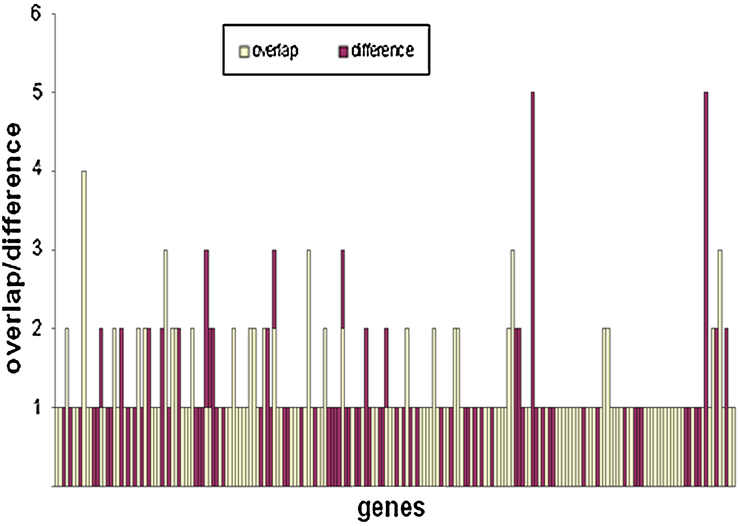
Our reconstructed model contained 449 edges (interactions), of which 298 belong to the published interaction set. The appendix contains the network topology, list of regulation functions, and list of cohorts (the appendix is available at the authors' website: http://acgt.cs.tau.ac.il/modent). Since we picked regulators to minimize the discrepancies with expression data, whereas the reported interactions were based on binding assays, we expected to see a different distribution of regulator-regulatee edges, and this was indeed the case (Fig. 3). Some of these differences are attributed to the false positives and false negatives in the reported interactions, although a true positive will not be inferred without proper expression data. For example, if we know that R regulates G, but in all the available expression profiles R is knocked down, we will not be able to use our knowledge in a model. Similarly, if the reported interactions are insufficient to produce a regulation function that satisfactorily predicts the target gene's level, unreported interactions need to be selected. The lower frame of Figure 3 shows that, for the ESC network, often one of the latter cases applied. Figure 4 illustrates the number of common target genes for each pair of regulators. Figure 5 illustrates the cohorts and their regulators; as can be seen, the TFs Pou5f1 and Sox2 regulate the two largest cohorts, while each of Nanog, Esrrb, Tcf7, and Etv5 regulate cohorts of intermediate size. Four cohorts are each regulated by four regulators, including Pou5f1, Rnf2, Zfp281, Dax1, Etv5, Sox2, Nr5a2, Phc1, and Otx2. It is reasonable to assume that genes that have more regulators are subjected to a more complex regulatory program, and therefore may have roles in more specific contexts compared to other genes; a better understanding of this network's behavior requires analysis of the dynamics involved.

FIG. 3.
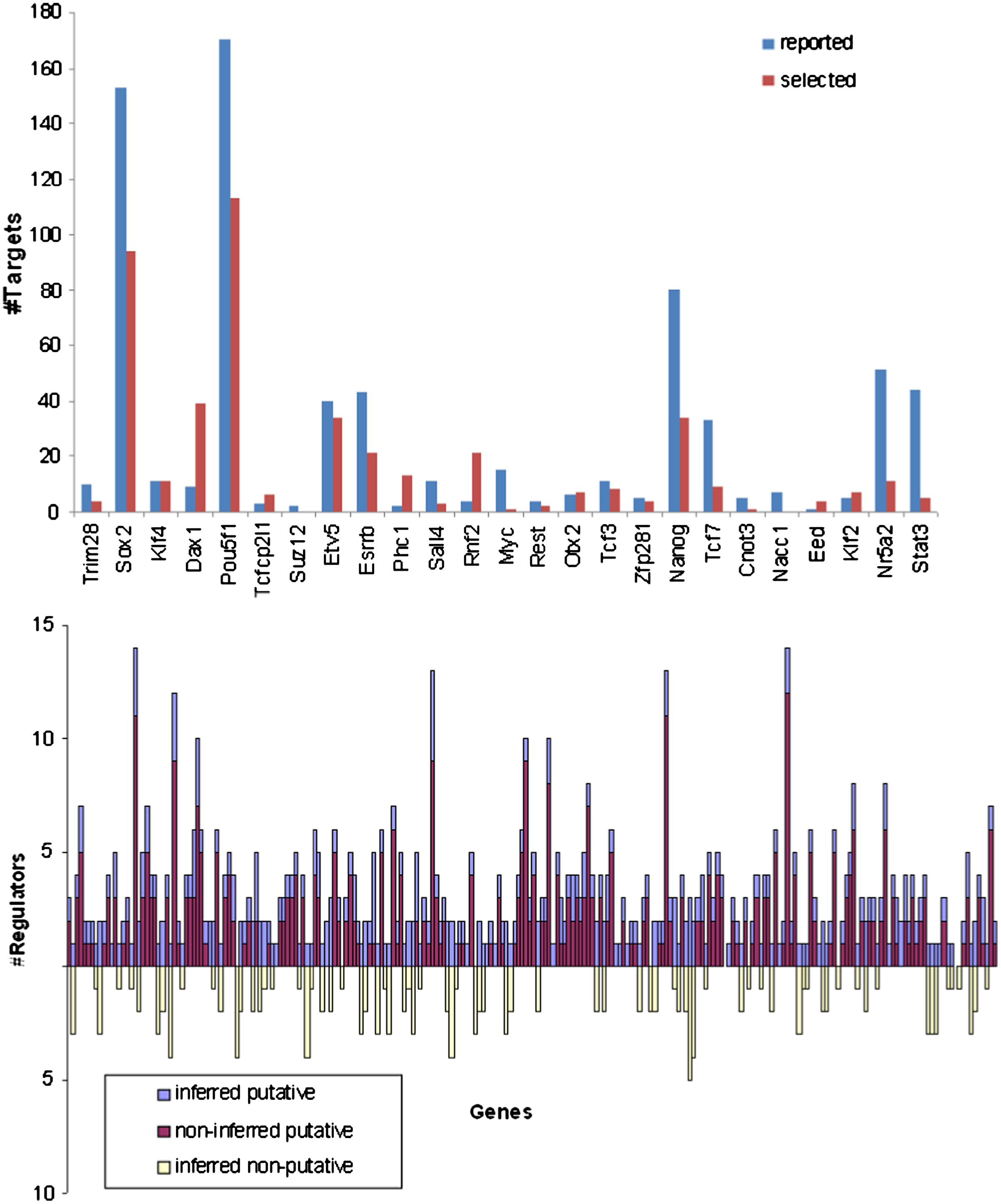
Comparison of reported interactions and interactions selected from expression profiles. Top frame: The number of reported targets compared to the number of selected targets for every transcription factor (TF). Bottom frame: For every gene, the number of reported TFs that were selected, the number of reported TFs that were not selected, and the number of unreported TFs that were selected. For clarity, the gene names were omitted.

FIG. 4.
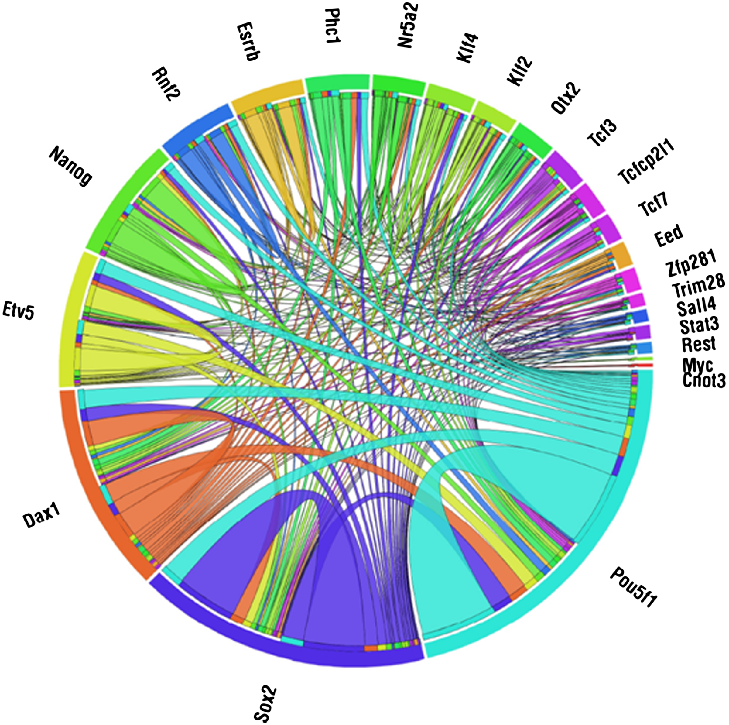
The number of common target genes for each pair of transcription factors (TFs). The colored arcs along the circumference indicate the inferred targets of TFs where, for clarity, each TF is represented by a different color. The internal arcs connect two groups of targets of two TFs and are colored by one of the two colors of the TFs. The size of an internal arc between two TFs is proportional to the number of common targets they share. An internal arc from a TF to itself indicates the total number of target genes of that TF. The figure was generated using Circos.

FIG. 5.
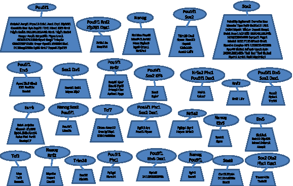
Cohorts and their sets of regulators. Each cohort is represented by a trapezoid, and the corresponding set of regulators is represented by an ellipse that is connected to its cohort's trapezoid. The names of the genes or regulators that belong to each set are given inside the shapes.

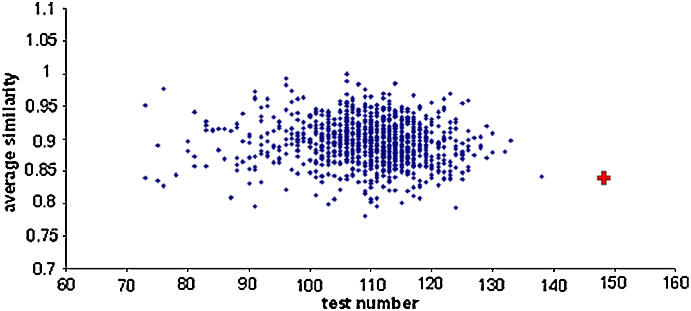
We turned to the dataset of Young and colleagues, found in Marson et al. (2008), to assess the quality of the selected interactions. In this study, ChIP-seq technique was used to measure binding of five TFs: Pou5f1, Sox2, Nanog, Tcf3, and Suz12, to regulatory regions of 200 genes in our network. The dataset corresponds to a 200 × 5 Boolean matrix M, in which the entry in the i^th row and the j^th column is 1 if TF j (1 ≤ j ≤ 5) binds gene i according to the ChIP-seq data. Now if S is the set of regulators of gene i in the reconstructed model, we define the similarity between S and row i in the matrix M as \documentclass{aastex} \usepackage{amsbsy} \usepackage{amsfonts} \usepackage{amssymb} \usepackage{bm} \usepackage{mathrsfs} \usepackage{pifont} \usepackage{stmaryrd} \usepackage{textcomp} \usepackage{portland, xspace} \usepackage{amsmath, amsxtra} \pagestyle{empty} \DeclareMathSizes {10} {9} {7} {6} \begin{document} $$ \frac { \sum \limits_ { j \in S } M [ i , j ] } { \mid S \mid }$$\end{document} . The average similarity between the regulators of a gene in the reconstructed model and the matrix M was 0.63. To assess the significance of this result, we randomly permuted each row in the matrix M independently and computed the average similarity. By repeating the randomization 10,000 times we conclude that this overlap value is significant at p-value < 10⁻⁴ (Fig. 6). Figure 7 compares the number of common regulators and the number of different regulators for each gene in the inferred model and in Marson et al. (2008).

FIG. 6.
Comparison of inferred and measured transcription factor (TF)–gene interactions. The average similarity of TF–gene interactions between the inferred network and the ChIP-seq interactions reported by Young et al., found in Marson et al. (2008), for five TFs was computed for randomized and real datasets. The figure shows the values for 10,000 random permutations of the Chip-seq dataset of Marson et al. (2008) and for the real dataset. Each blue dot represents the values obtained for one permutation. The red plus sign corresponds to the score of the real dataset.

FIG. 7.
The number of common transcription factors (TFs) and different TFs for each gene in the inferred network and the dataset of Marson et al. (2008).

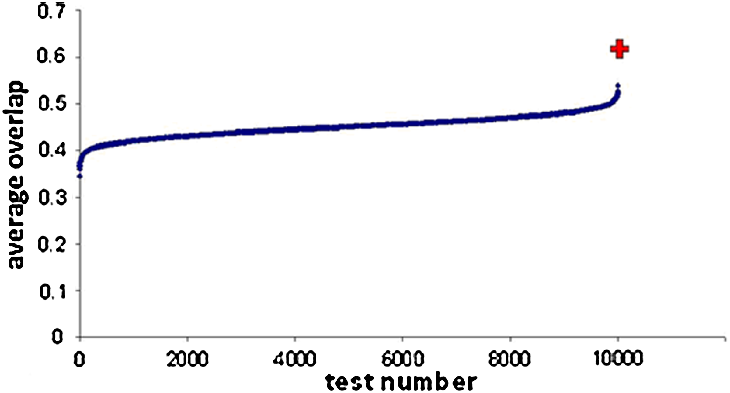
We call a set of genes that have the exact same regulators a cohort. We wanted to test whether genes that share the same set of regulators tend to have the same regulatory logic. We define similarity between two regulation functions as the fraction of inputs that produce identical outputs. The average similarity in a cohort is the average similarity between pairs of genes in that cohort. In order to eliminate genes whose levels may have been incorrectly modeled, genes with truth tables that were on average less than 50% similar to all other genes in the cohort were excluded. This filtering left 144 out of 184 genes that belong to cohorts, excluding no more than a third of the genes in any cohort. The average percentage of logic similarity that was obtained among the remaining genes in each cohort is 84%. To assess the significance, we permuted edges in the network of Young and colleagues, found in Marson et al. (2008), by conducting a long series of edge swaps, a process that preserves the degree of each node, and then reconstructing the model given the permuted network (Ulitsky, et al, 2010). For every permutation, the average percentage of cohort similarity and the number of excluded genes were computed as described above, and compared to the values that were obtained for the model. We considered a solution as scoring better only if (i) the similarity was equal or higher and (ii) the number of genes that were included in cohorts was equal or higher. Both conditions must be taken into account, since otherwise similarity is maximized by reducing the number and size of cohorts through gene exclusion or edge swap. Repeating the process 10⁵ times showed that the logic similarity was significant at p-value < 10⁻⁵. Figure 8 compares the scores of 1000 random permutations and the score obtained by the real topology. In order to make sure that our exclusion scheme does not generate any biases, we repeated the test by applying criteria (i) and (ii) without excluding genes from cohorts and obtained a p-value of 1.1·10⁻⁴. In order for the simulation to run sufficiently fast, a speed-up of the selection procedure was used in which regulators are added incrementally to the regulators set as long as the entropy improves significantly. A similar speedup was used in Hashimoto et al. (2003), using discrete data and a different score.

FIG. 8.
Logic similarity and cohort sizes for randomized and real networks. The figure shows the values for 1000 random permutations of the embryonic stem cell (ESC) network and for the real topology. Each blue dot is a value obtained for one permutation, where the y-coordinate is the within-cohort similarity and the x-coordinate is the number of genes in cohorts of size at least 2. The red plus sign corresponds to the score of the real topology.

Figure 9 shows the similarity of regulation function of all the genes in the network. The network is seen to contain cohorts with highly similar regulation functions. There are some similarities in the regulation functions of genes that belong to different cohorts (depicted as edges that cross the interior of the circle), due perhaps to reuse of certain “regulatory logic motifs” in gene regulation (Milo et al., 2002).

FIG. 9.
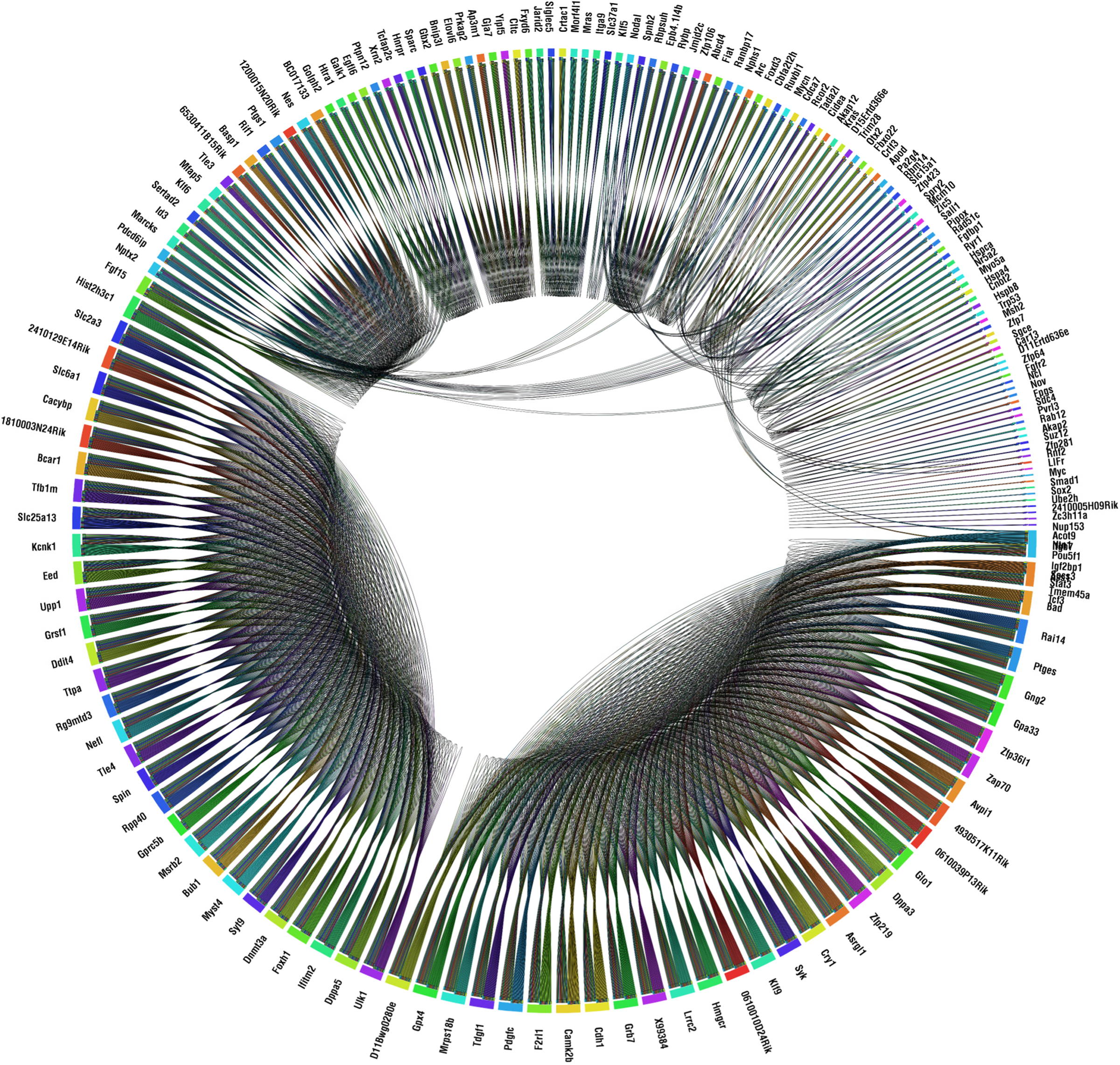
The similarity of regulation functions for every pair of genes that have at least one common regulator. Similarity is measured as the fraction of identical outputs. Similarity of regulation functions of genes that have a different number of regulators are also compared: each output of the function with less regulators is compared to several outputs of the function with more regulators. For clarity, only genes that share >75% similarity are connected. The figure was generated using Circos.

These results are in line with the common assumption that regulatory logics within cohorts are similar, and also with the more general observation that networks contain “reusable components” (Milo et al., 2002). The term “reusable components” means that regulatory elements can be used similarly for different parts of the network. Segal et al. (2003) based their method on this assumption. Since our method does not impose any constraints on logic within cohorts and we still observe a high level of identical regulation within cohorts, we conclude that the reconstructed model is reasonably reliable.

4. Discussion

We have presented an algorithm for constructing a logical model and resolving discrepancies between the model and experimental data. After demonstrating that the general problem of resolving discrepancies is computationally hard and there is probably no efficient algorithm that solves it, we adopted a probabilistic approach to the network reconstruction problem. We developed an algorithm that uses reported interactions and expression data to select a set of regulators for each gene, and that resolves discrepancies in the resulting logical model. We used our algorithm to construct a logical model of the mouse ESC GRN. The model supports the notion that genes which share the same regulators have similar regulatory logics.

Unlike Dimitrova et al. (2010) and other discretization methods, our algorithm refrains from directly discretizing the data, thereby avoiding the errors that are inherent to this process and the intractability of minimizing them. Instead, it assigns a probability to each discrete value and adjusts the input real values to improve model consistency, as reflected by the conditional entropy. Other methods that use information theory for selecting regulators discretize the data, but do not provide a means of discrepancy resolution (Liang et al., 1998; Lopes et al., 2008). Our algorithm can be applied when using only expression profiles as input, but can also utilize information on putative regulations (e.g., from ChIP-chip or ChIP-seq data) to improve the prediction. Given a set of such putative interactions, it can reject those that lack support in expression data. A disadvantage of our method is that we normalize the expression profiles of all the genes using the same parameters, which may be inferior to preprocessing using gene-specific parameters. Another disadvantage is that the inferred discrete logic is a necessary oversimplification of the biological reality. Finally, as the general problem is computationally hard, we resort to heuristics, and at least for some instances of the problem, we may not find the optimal solution.

At this point, it is natural to ask whether one can obtain logical models that are sufficiently accurate. A model that contains even a small number of errors can produce erroneous predictions. Theoretical examples in which a small error in the model has a large impact on its predictions are easily found (Lorenz, 1993). Further research is required to determine whether domain-specific algorithms can produce accurate logical models. Another approach to the problem is developing algorithms that analyze a model without trying to resolve all the ambiguities in it (Karlebach and Shamir, 2010).

The probabilistic approach to discretization that we describe could be applied to other purposes in bioinformatics. Because discretization of expression data is used in methods such as clustering (Ben-Dor et al., 1999; Koyuturk et al., 2004) and feature selection (Saeys et al., 2007; Akutsu and Miyano, 2001), resolving discrepancies in discretized expression data can be performed as a preliminary step.

We intend to proceed with the analysis of the mouse ESC model, including its dynamic behavior and the effect of perturbations. Our reconstruction algorithm should be tested on other datasets in order to further characterize its advantages and disadvantages. Reconstruction of accurate logical models and their use for generating useful predictions are objectives that require further exploration.

Footnotes

Acknowledgments

We would like to thank Qing Zhou, Wing Wong, and Avi Ma'ayan for help and advice with data that were used in this work, and Hershel Safer for helpful comments on this manuscript. This study was supported in part by a grant to the APO-SYS consortium from the European Community's Seventh Framework Programme. G.K. was supported in part by a fellowship from the Edmond J. Safra Bioinformatics Program at Tel Aviv University, Israel.

Disclosure Statement

No competing financial interests exist.

References

Akutsu

, Miyano

2001. Selecting informative genes for cancer classification using gene expression data. Proc. IEEE-EURASIP Workshop Nonlinear Signal Image Process., 3–6.

Akutsu

, Tamura

, Horimoto

2009. Completing networks using observed data. Algorithmic Learn. Theor., 126–140.

Akutsu

, Miyano

, Kuhara

1999. Identification of genetic networks from a small number of gene expression patterns under the Boolean network model. Pac. Symp. Biocomput., 17–28.

Ben-Dor

, Shamir

, Yakhini

1999. Clustering gene expression patterns. J. Comput. Biol., 6:281–297.

Chickarmane

, Troein

, Nuber

U.A.

et al. 2006. Transcriptional dynamics of the embryonic stem cell switch. PLoS Comput. Biol., 2:e123.

Cox

R.S.

3rd , Surette

M.G.

, Elowitz

M.B.

2007. Programming gene expression with combinatorial promoters. Mol. Syst. Biol., 3:145.

Dimitrova

E.S.

, Licona

M.P.

, McGee

et al. 2010. Discretization of time series data. J. Comput. Biol., 17:853–868.

Glass

, Kauffman

1973. The logical analysis of continuous, non-linear biochemical control networks. J. Theor. Biol., 39:103–129.

Hashimoto

, Dougherty

, Brun

et al. 2003. Efficient selection of feature sets possessing high coefficients of determination based on incremental determinations. Signal Process., 83:695–712.

10.

Ivanova

, Dobrin

, Lu

et al. 2006. Dissecting self-renewal in stem cells with RNA interference. Nature, 442:533–538.

11.

Karlebach

, Shamir

2010. Minimally perturbing a gene regulatory network to avoid a disease phenotype: the glioma network as a test case. BMC Syst. Biol., 4:15.

12.

Karlebach

, Shamir

2008. Modelling and analysis of gene regulatory networks. Nat. Rev. Mol. Cell Biol., 9:770–780.

13.

Karp

1972. Reducibility Among Combinatorial Problems. Complexity of Computer Computations, 85–103.

14.

Koyuturk

, Szpankowski

, Grama

2004. Biclustering gene-feature matrices for statistically significant dense patterns. Proc. IEEE Comput. Syst. Bioinformatics Conf. (CSB’04), 480–484.

15.

Krzywinski

, Schein

, Birol

et al. 2009. Circos: an information aesthetic for comparative genomics. Genome Res., 19:1639–1645.

16.

Lähdesmäki

, Shmulevich

, Yli-Harja . 2003. On learning gene regulatory networks under the Boolean network model. Machine Learn., 52:147–167.

17.

Liang

, Fuhrman

, Somogyi

1998. Reveal, a general reverse engineering algorithm for inference of genetic network architectures. Pac. Symp. Biocomput., 18–29.

18.

Lopes

F.M.

, Martins

D.C.

Jr. , Cesar

R.M.

Jr.

2008. Feature selection environment for genomic applications. BMC Bioinform., 9:451.

19.

Lorenz

E.N.

1993. The Essence of Chaos. University of Washington Press: Seattle.

20.

MacArthur

, Ma'ayan

, Lemischka

2009. Systems biology of stem cell fate and cellular reprogramming. Nat. Rev. Mol. Cell Biol., 10:672–681.

21.

Marson

, Levine

S.S.

, Cole

M.F.

et al. 2008. Connecting microRNA genes to the core transcriptional regulatory circuitry of embryonic stem cells. Cell, 134:521–533.

22.

Mayo

A.E.

, Setty

, Shavit

et al. 2006. Plasticity of the cis-regulatory input function of a gene. PLoS Biol., 4:e45.

23.

Milo

, Shen-Orr

, Itzkovitz

et al. 2002. Network motifs: simple building blocks of complex networks. Science, 298:824–827.

24.

Novershtern

, Subramanian

, Lawton

L.N.

et al. 2011. Densely interconnected transcriptional circuits control cell states in human hematopoiesis. Cell, 144:296–309.

25.

Saeys

, Inza

, Larranaga

2007. A review of feature selection techniques in bioinformatics. Bioinformatics, 23:2507–2517.

26.

Segal

, Shapira

, Regev

et al. 2003. Module networks: identifying regulatory modules and their condition-specific regulators from gene expression data. Nat. Genet., 34:166–176.

27.

Shamir

, Tanay

2003. Modeling transcription programs: inferring binding site activity and dose-response model optimization. Proc.RECOMB'03.

28.

Thomas

1973. Boolean formalization of genetic control circuits. J. Theor. Biol., 42:563–585.

29.

Tsong

A.E.

, Tuch

B.B.

, Li

et al. 2006. Evolution of alternative transcriptional circuits with identical logic. Nature, 443:415–420.

30.

Ulitsky

, Laurent

L.C.

, Shamir

2010. Towards computational prediction of microRNA function and activity. Nucleic Acids Res., 38:e160.

31.

, Schaniel

, Lemischka

I.R.

et al. 2010. Toward a complete in silico, multi-layered embryonic stem cell regulatory network. Wiley Interdiscip. Rev. Syst. Biol. Med., 2:708–733.

32.

Zhou

, Chipperfield

, Melton

et al. 2007. A gene regulatory network in mouse embryonic stem cells. Proc. Natl. Acad. Sci. U.S.A., 104:16438–16443.