Many approaches to compute the genomic distance are still limited to genomes with the same content, without duplicated markers. However, differences in the gene content are frequently observed and can reflect important evolutionary aspects. While duplicated markers can hardly be handled by exact models, when duplicated markers are not allowed, a few polynomial time algorithms that include genome rearrangements, insertions and deletions were already proposed. In an attempt to improve these results, in the present work we give the first linear time algorithm to compute the distance between two multichromosomal genomes with unequal content, but without duplicated markers, considering insertions, deletions and double cut and join (DCJ) operations. We derive from this approach algorithms to sort one genome into another one also using DCJ operations, insertions and deletions. The optimal sorting scenarios can have different compositions and we compare two types of sorting scenarios: one that maximizes and one that minimizes the number of DCJ operations with respect to the number of insertions and deletions. We also show that, although the triangle inequality can be disrupted in the proposed genomic distance, it is possible to correct this problem adopting a surcharge on the number of non-common markers. We use our method to analyze six species of Rickettsia, a group of obligate intracellular parasites, and identify preliminary evidence of clusters of deletions.
1. Introduction
The distance between two genomes is often computed using only the common markers, that occur in both genomes (Hannenhalli and Pevzner, 1995; Yancopoulos et al., 2005; Bergeron et al., 2006; Braga and Stoye, 2010). However, genomes with the same content are rare, and differences in gene content may reflect important evolutionary aspects. Interesting examples are bacteria which are obligate intracellular parasites. The genomes of such bacteria are observed to have a reductive evolution, that is the process by which genomes shrink and undergo extreme levels of gene degradation and loss (Andersson and Kurland, 1998). Approaches that are able to handle genomes with unequal content could give valuable hints on the evolution of such organisms.
While duplicated markers can hardly be handled by exact models (Sankoff, 1999; Bryant, 2001; Marron et al., 2004; Bader, 2010), some polynomial time approaches that are able to deal with insertions and deletions were proposed. In this context, El-Mabrouk (2001) introduced a method to compare unichromosomal genomes with unequal content, but without duplicated markers, considering inversions, insertions and deletions, such that a block of contiguous markers can be inserted or deleted at once. Two algorithms were provided, an exact one, which deals with insertions and deletions asymmetrically, and a heuristic that is able to handle all operations symmetrically.
In the present work, we develop a linear time symmetric approach to compare multichromosomal genomes with unequal content, but without duplicated markers, also allowing a block of contiguous markers to be inserted or deleted at once. In addition to insertions and deletions, we consider double cut and join (DCJ) operations, that allow us to represent most large scale rearrangements, such as inversions, translocations, fusions and fissions, that can occur in genomes (Yancopoulos et al., 2005; Bergeron et al., 2006). We borrow some ideas from a study of Yancopoulos and Friedberg (2009), but in our model we provide a clear separation between insertions, deletions and DCJ operations. We then derive algorithms to sort one genome into another one, showing that the optimal sorting scenarios can have different compositions with respect to the number of each type of operation and propose two types of sorting scenarios: one that minimizes the number of DCJ operations (respectively maximizes the number of insertions and deletions) and one that minimizes the number of insertions and deletions (respectively maximizes the number of DCJ operations).
We use our method to analyze six species of Rickettsia (Blanc et al., 2007), a group of obligate intracellular parasites, and are able to identify preliminary evidence of clusters of deletions in the analyzed genomes. Furthermore, we show that the triangle inequality can be disrupted in our model, but this problem can be corrected a posteriori by applying a surcharge on the number of non-common markers.
This article is an extension of the results recently presented in two subsequent works (Braga, 2010; Braga et al., 2010) and is organized as follows. In Section 2, we give the basic definitions of our model, and in Section 3, we develop the indel-potential of two genomes, a property that allows us to obtain a good upper bound to the genomic distance with DCJ and indel operations. Then, in Section 4, we obtain an exact formula for the distance, also showing that it can be computed in linear time, while in Section 5, we derive algorithms to sort genomes with DCJ and indel operations. In Section 6, we apply our method to analyze the evolution of Rickettsia. In Section 7, we propose a surcharge to establish the triangle inequality, and, finally, in Section 8 we summarize our results.
2. Definitions
We analyze genomes with unequal content but without duplicated markers. Each genome is possibly composed of linear and circular chromosomes and can be represented by a set of strings as follows. From each chromosome \documentclass{aastex}\usepackage{amsbsy}\usepackage{amsfonts}\usepackage{amssymb}\usepackage{bm}\usepackage{mathrsfs}\usepackage{pifont}\usepackage{stmaryrd}\usepackage{textcomp}\usepackage{portland, xspace}\usepackage{amsmath, amsxtra}\pagestyle{empty}\DeclareMathSizes{10}{9}{7}{6}\begin{document}
$${\cal C}$$
\end{document} of each genome, we can build a string s, obtained by the concatenation of all markers in \documentclass{aastex}\usepackage{amsbsy}\usepackage{amsfonts}\usepackage{amssymb}\usepackage{bm}\usepackage{mathrsfs}\usepackage{pifont}\usepackage{stmaryrd}\usepackage{textcomp}\usepackage{portland, xspace}\usepackage{amsmath, amsxtra}\pagestyle{empty}\DeclareMathSizes{10}{9}{7}{6}\begin{document}
$${\cal C}$$
\end{document}, read in any of the two directions. Each marker g is a DNA fragment and is represented by the symbol g, if it is read in direct orientation, or by the symbol \documentclass{aastex}\usepackage{amsbsy}\usepackage{amsfonts}\usepackage{amssymb}\usepackage{bm}\usepackage{mathrsfs}\usepackage{pifont}\usepackage{stmaryrd}\usepackage{textcomp}\usepackage{portland, xspace}\usepackage{amsmath, amsxtra}\pagestyle{empty}\DeclareMathSizes{10}{9}{7}{6}\begin{document}
$$\overline{g}$$
\end{document}, if it is read in reverse orientation. Each end of a linear chromosome is called a telomere, represented by the symbol ∘. Thus, if \documentclass{aastex}\usepackage{amsbsy}\usepackage{amsfonts}\usepackage{amssymb}\usepackage{bm}\usepackage{mathrsfs}\usepackage{pifont}\usepackage{stmaryrd}\usepackage{textcomp}\usepackage{portland, xspace}\usepackage{amsmath, amsxtra}\pagestyle{empty}\DeclareMathSizes{10}{9}{7}{6}\begin{document}
$${\cal C}$$
\end{document} is linear, it is represented by ∘s∘. If \documentclass{aastex}\usepackage{amsbsy}\usepackage{amsfonts}\usepackage{amssymb}\usepackage{bm}\usepackage{mathrsfs}\usepackage{pifont}\usepackage{stmaryrd}\usepackage{textcomp}\usepackage{portland, xspace}\usepackage{amsmath, amsxtra}\pagestyle{empty}\DeclareMathSizes{10}{9}{7}{6}\begin{document}
$${\cal C}$$
\end{document} is circular, it is simply represented by s (we can start to build s in any symbol of \documentclass{aastex}\usepackage{amsbsy}\usepackage{amsfonts}\usepackage{amssymb}\usepackage{bm}\usepackage{mathrsfs}\usepackage{pifont}\usepackage{stmaryrd}\usepackage{textcomp}\usepackage{portland, xspace}\usepackage{amsmath, amsxtra}\pagestyle{empty}\DeclareMathSizes{10}{9}{7}{6}\begin{document}
$${\cal C}$$
\end{document}).
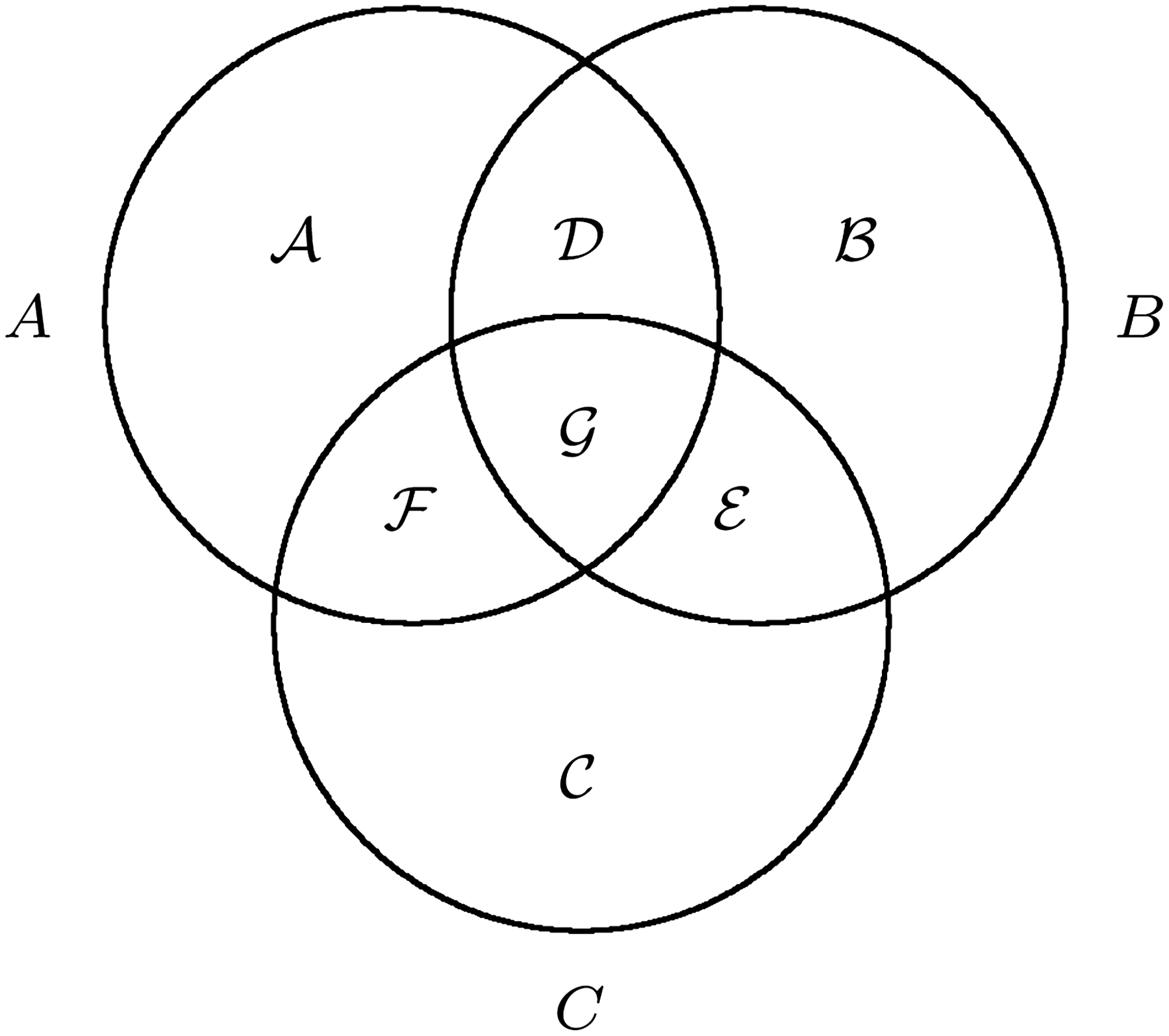
Given two different genomes A and B, we denote by \documentclass{aastex}\usepackage{amsbsy}\usepackage{amsfonts}\usepackage{amssymb}\usepackage{bm}\usepackage{mathrsfs}\usepackage{pifont}\usepackage{stmaryrd}\usepackage{textcomp}\usepackage{portland, xspace}\usepackage{amsmath, amsxtra}\pagestyle{empty}\DeclareMathSizes{10}{9}{7}{6}\begin{document}
$${\cal G}$$
\end{document} the “reduced” genome (El-Mabrouk, 2001), that is the set of markers that occur once in A and once in B. Moreover, the set \documentclass{aastex}\usepackage{amsbsy}\usepackage{amsfonts}\usepackage{amssymb}\usepackage{bm}\usepackage{mathrsfs}\usepackage{pifont}\usepackage{stmaryrd}\usepackage{textcomp}\usepackage{portland, xspace}\usepackage{amsmath, amsxtra}\pagestyle{empty}\DeclareMathSizes{10}{9}{7}{6}\begin{document}
$${\cal A}$$
\end{document} contains the markers that occur only in A and the set \documentclass{aastex}\usepackage{amsbsy}\usepackage{amsfonts}\usepackage{amssymb}\usepackage{bm}\usepackage{mathrsfs}\usepackage{pifont}\usepackage{stmaryrd}\usepackage{textcomp}\usepackage{portland, xspace}\usepackage{amsmath, amsxtra}\pagestyle{empty}\DeclareMathSizes{10}{9}{7}{6}\begin{document}
$${\cal B}$$
\end{document} contains the markers that occur only in B. Observe that the sets \documentclass{aastex}\usepackage{amsbsy}\usepackage{amsfonts}\usepackage{amssymb}\usepackage{bm}\usepackage{mathrsfs}\usepackage{pifont}\usepackage{stmaryrd}\usepackage{textcomp}\usepackage{portland, xspace}\usepackage{amsmath, amsxtra}\pagestyle{empty}\DeclareMathSizes{10}{9}{7}{6}\begin{document}
$${\cal G}, \ {\cal A} \ {\rm and} \ {\cal B}$$
\end{document} are disjoint. An example of a pair of genomes is given in Figure 1.
(A, B) For genomes \documentclass{aastex}\usepackage{amsbsy}\usepackage{amsfonts}\usepackage{amssymb}\usepackage{bm}\usepackage{mathrsfs}\usepackage{pifont}\usepackage{stmaryrd}\usepackage{textcomp}\usepackage{portland, xspace}\usepackage{amsmath, amsxtra}\pagestyle{empty}\DeclareMathSizes{10}{9}{7}{6}\begin{document}
$$A = \{ \circ axec \circ, \circ d \overline{y}b \circ, \circ z \overline{w} \circ \}$$
\end{document}, composed of three linear chromosomes, and \documentclass{aastex}\usepackage{amsbsy}\usepackage{amsfonts}\usepackage{amssymb}\usepackage{bm}\usepackage{mathrsfs}\usepackage{pifont}\usepackage{stmaryrd}\usepackage{textcomp}\usepackage{portland, xspace}\usepackage{amsmath, amsxtra}\pagestyle{empty}\DeclareMathSizes{10}{9}{7}{6}\begin{document}
$$B = \{ \circ abcdve \circ \} $$
\end{document}, composed of one single chromosome, we have \documentclass{aastex}\usepackage{amsbsy}\usepackage{amsfonts}\usepackage{amssymb}\usepackage{bm}\usepackage{mathrsfs}\usepackage{pifont}\usepackage{stmaryrd}\usepackage{textcomp}\usepackage{portland, xspace}\usepackage{amsmath, amsxtra}\pagestyle{empty}\DeclareMathSizes{10}{9}{7}{6}\begin{document}
$${\cal G} = \{a, b, c, d, e \}, \ {\cal A} = \{x, y, z, w \} \ {\rm and} \ {\cal B} = \{v \}$$
\end{document}.
Before introducing the indel operation, in the following three subsections we give some important concepts of the DCJ model, that are generalizations of definitions introduced by Bergeron et al. (2006).
Given two different genomes A and B, recall that \documentclass{aastex}\usepackage{amsbsy}\usepackage{amsfonts}\usepackage{amssymb}\usepackage{bm}\usepackage{mathrsfs}\usepackage{pifont}\usepackage{stmaryrd}\usepackage{textcomp}\usepackage{portland, xspace}\usepackage{amsmath, amsxtra}\pagestyle{empty}\DeclareMathSizes{10}{9}{7}{6}\begin{document}
$${\cal G}$$
\end{document} is the set of markers that occur once in A and once in B. For each marker \documentclass{aastex}\usepackage{amsbsy}\usepackage{amsfonts}\usepackage{amssymb}\usepackage{bm}\usepackage{mathrsfs}\usepackage{pifont}\usepackage{stmaryrd}\usepackage{textcomp}\usepackage{portland, xspace}\usepackage{amsmath, amsxtra}\pagestyle{empty}\DeclareMathSizes{10}{9}{7}{6}\begin{document}
$$g \in {\cal G}$$
\end{document}, denote its two extremities by gt (tail) and gh (head). Then, a \documentclass{aastex}\usepackage{amsbsy}\usepackage{amsfonts}\usepackage{amssymb}\usepackage{bm}\usepackage{mathrsfs}\usepackage{pifont}\usepackage{stmaryrd}\usepackage{textcomp}\usepackage{portland, xspace}\usepackage{amsmath, amsxtra}\pagestyle{empty}\DeclareMathSizes{10}{9}{7}{6}\begin{document}
$${\cal G}$$
\end{document}-adjacency in genome A (respectively in genome B) is in general a linear string v = γ1ℓγ2, such that γ1 and γ2 are telomeres or extremities of markers of \documentclass{aastex}\usepackage{amsbsy}\usepackage{amsfonts}\usepackage{amssymb}\usepackage{bm}\usepackage{mathrsfs}\usepackage{pifont}\usepackage{stmaryrd}\usepackage{textcomp}\usepackage{portland, xspace}\usepackage{amsmath, amsxtra}\pagestyle{empty}\DeclareMathSizes{10}{9}{7}{6}\begin{document}
$${\cal G}$$
\end{document} and ℓ, the substring composed of the markers that are between γ1 and γ2 in A (respectively in B), contains no marker that also belongs to \documentclass{aastex}\usepackage{amsbsy}\usepackage{amsfonts}\usepackage{amssymb}\usepackage{bm}\usepackage{mathrsfs}\usepackage{pifont}\usepackage{stmaryrd}\usepackage{textcomp}\usepackage{portland, xspace}\usepackage{amsmath, amsxtra}\pagestyle{empty}\DeclareMathSizes{10}{9}{7}{6}\begin{document}
$${\cal G}$$
\end{document}. The substring ℓ is said to be the label of v, and the extremities γ1 and γ2 are said to be \documentclass{aastex}\usepackage{amsbsy}\usepackage{amsfonts}\usepackage{amssymb}\usepackage{bm}\usepackage{mathrsfs}\usepackage{pifont}\usepackage{stmaryrd}\usepackage{textcomp}\usepackage{portland, xspace}\usepackage{amsmath, amsxtra}\pagestyle{empty}\DeclareMathSizes{10}{9}{7}{6}\begin{document}
$${\cal G}$$
\end{document}-adjacent. If ℓ is a non-empty string, v is said to be labeled, otherwise v is said to be clean.
Observe that a \documentclass{aastex}\usepackage{amsbsy}\usepackage{amsfonts}\usepackage{amssymb}\usepackage{bm}\usepackage{mathrsfs}\usepackage{pifont}\usepackage{stmaryrd}\usepackage{textcomp}\usepackage{portland, xspace}\usepackage{amsmath, amsxtra}\pagestyle{empty}\DeclareMathSizes{10}{9}{7}{6}\begin{document}
$${\cal G}$$
\end{document}-adjacency γ1ℓγ2 can also be represented by \documentclass{aastex}\usepackage{amsbsy}\usepackage{amsfonts}\usepackage{amssymb}\usepackage{bm}\usepackage{mathrsfs}\usepackage{pifont}\usepackage{stmaryrd}\usepackage{textcomp}\usepackage{portland, xspace}\usepackage{amsmath, amsxtra}\pagestyle{empty}\DeclareMathSizes{10}{9}{7}{6}\begin{document}
$$\gamma_2 \overline{\ell} \gamma_1$$
\end{document}. Moreover, a labeled \documentclass{aastex}\usepackage{amsbsy}\usepackage{amsfonts}\usepackage{amssymb}\usepackage{bm}\usepackage{mathrsfs}\usepackage{pifont}\usepackage{stmaryrd}\usepackage{textcomp}\usepackage{portland, xspace}\usepackage{amsmath, amsxtra}\pagestyle{empty}\DeclareMathSizes{10}{9}{7}{6}\begin{document}
$${\cal G}$$
\end{document}-adjacency v = ∘ℓ∘ in genome A (or B) indicates that A (or B) contains a linear chromosome composed only of markers that are not in \documentclass{aastex}\usepackage{amsbsy}\usepackage{amsfonts}\usepackage{amssymb}\usepackage{bm}\usepackage{mathrsfs}\usepackage{pifont}\usepackage{stmaryrd}\usepackage{textcomp}\usepackage{portland, xspace}\usepackage{amsmath, amsxtra}\pagestyle{empty}\DeclareMathSizes{10}{9}{7}{6}\begin{document}
$${\cal G}$$
\end{document}, that is, v corresponds to a whole linear chromosome. In the same way, a special case is a \documentclass{aastex}\usepackage{amsbsy}\usepackage{amsfonts}\usepackage{amssymb}\usepackage{bm}\usepackage{mathrsfs}\usepackage{pifont}\usepackage{stmaryrd}\usepackage{textcomp}\usepackage{portland, xspace}\usepackage{amsmath, amsxtra}\pagestyle{empty}\DeclareMathSizes{10}{9}{7}{6}\begin{document}
$${\cal G}$$
\end{document}-adjacency v = ℓ, that corresponds to a whole circular chromosome in A (or B), composed only of markers that are not in \documentclass{aastex}\usepackage{amsbsy}\usepackage{amsfonts}\usepackage{amssymb}\usepackage{bm}\usepackage{mathrsfs}\usepackage{pifont}\usepackage{stmaryrd}\usepackage{textcomp}\usepackage{portland, xspace}\usepackage{amsmath, amsxtra}\pagestyle{empty}\DeclareMathSizes{10}{9}{7}{6}\begin{document}
$${\cal G}$$
\end{document}. This is the only case of a \documentclass{aastex}\usepackage{amsbsy}\usepackage{amsfonts}\usepackage{amssymb}\usepackage{bm}\usepackage{mathrsfs}\usepackage{pifont}\usepackage{stmaryrd}\usepackage{textcomp}\usepackage{portland, xspace}\usepackage{amsmath, amsxtra}\pagestyle{empty}\DeclareMathSizes{10}{9}{7}{6}\begin{document}
$${\cal G}$$
\end{document}-adjacency in which we have a circular instead of a linear string.
Two genomes A and B can then be represented by the sets \documentclass{aastex}\usepackage{amsbsy}\usepackage{amsfonts}\usepackage{amssymb}\usepackage{bm}\usepackage{mathrsfs}\usepackage{pifont}\usepackage{stmaryrd}\usepackage{textcomp}\usepackage{portland, xspace}\usepackage{amsmath, amsxtra}\pagestyle{empty}\DeclareMathSizes{10}{9}{7}{6}\begin{document}
$$V_{\cal G} (A) \ {\rm and} \ V_{\cal G} (B)$$
\end{document}, containing their \documentclass{aastex}\usepackage{amsbsy}\usepackage{amsfonts}\usepackage{amssymb}\usepackage{bm}\usepackage{mathrsfs}\usepackage{pifont}\usepackage{stmaryrd}\usepackage{textcomp}\usepackage{portland, xspace}\usepackage{amsmath, amsxtra}\pagestyle{empty}\DeclareMathSizes{10}{9}{7}{6}\begin{document}
$${\cal G}$$
\end{document}-adjacencies. For the genomes in Figure 1, we have \documentclass{aastex}\usepackage{amsbsy}\usepackage{amsfonts}\usepackage{amssymb}\usepackage{bm}\usepackage{mathrsfs}\usepackage{pifont}\usepackage{stmaryrd}\usepackage{textcomp}\usepackage{portland, xspace}\usepackage{amsmath, amsxtra}\pagestyle{empty}\DeclareMathSizes{10}{9}{7}{6}\begin{document}
$${\cal G} = \{a, b, c, d, e \}, V_{\cal G} (A) = \{ \circ a^t, a^h xe^t, e^h c^t, c^h \circ, \circ d^t, d^h \overline{y}b^t, b^h \circ, \circ\; z \overline{w} \circ \} \ {\rm and} \ V_{\cal G} (B) = \{ \circ a^t, a^h b^t, b^h c^t, c^h d^t, d^h ve^t, e^h \circ \}$$
\end{document}.
2.2. The DCJ operation
A cut performed on a genome A separates two adjacent markers of A. A cut affects a \documentclass{aastex}\usepackage{amsbsy}\usepackage{amsfonts}\usepackage{amssymb}\usepackage{bm}\usepackage{mathrsfs}\usepackage{pifont}\usepackage{stmaryrd}\usepackage{textcomp}\usepackage{portland, xspace}\usepackage{amsmath, amsxtra}\pagestyle{empty}\DeclareMathSizes{10}{9}{7}{6}\begin{document}
$${\cal G}$$
\end{document}-adjacency v of \documentclass{aastex}\usepackage{amsbsy}\usepackage{amsfonts}\usepackage{amssymb}\usepackage{bm}\usepackage{mathrsfs}\usepackage{pifont}\usepackage{stmaryrd}\usepackage{textcomp}\usepackage{portland, xspace}\usepackage{amsmath, amsxtra}\pagestyle{empty}\DeclareMathSizes{10}{9}{7}{6}\begin{document}
$$V_{\cal G} (A)$$
\end{document} as follows: if v is linear, the cut is done between two symbols of v, creating two open ends in two separate linear strings; if v is circular, the cut creates two open ends in one linear string. A double-cut and join or DCJ applied on a genome A is the operation that performs two cuts in \documentclass{aastex}\usepackage{amsbsy}\usepackage{amsfonts}\usepackage{amssymb}\usepackage{bm}\usepackage{mathrsfs}\usepackage{pifont}\usepackage{stmaryrd}\usepackage{textcomp}\usepackage{portland, xspace}\usepackage{amsmath, amsxtra}\pagestyle{empty}\DeclareMathSizes{10}{9}{7}{6}\begin{document}
$$V_{\cal G} (A)$$
\end{document}, creating four open ends, and joins these open ends in a different way. As an example, considering the genome A from Figure 1 and \documentclass{aastex}\usepackage{amsbsy}\usepackage{amsfonts}\usepackage{amssymb}\usepackage{bm}\usepackage{mathrsfs}\usepackage{pifont}\usepackage{stmaryrd}\usepackage{textcomp}\usepackage{portland, xspace}\usepackage{amsmath, amsxtra}\pagestyle{empty}\DeclareMathSizes{10}{9}{7}{6}\begin{document}
$${\cal G} = \{a, b, c, d, e \} $$
\end{document}, if we apply a DCJ on ahxet and \documentclass{aastex}\usepackage{amsbsy}\usepackage{amsfonts}\usepackage{amssymb}\usepackage{bm}\usepackage{mathrsfs}\usepackage{pifont}\usepackage{stmaryrd}\usepackage{textcomp}\usepackage{portland, xspace}\usepackage{amsmath, amsxtra}\pagestyle{empty}\DeclareMathSizes{10}{9}{7}{6}\begin{document}
$$d^h \overline{y}b^t$$
\end{document} of \documentclass{aastex}\usepackage{amsbsy}\usepackage{amsfonts}\usepackage{amssymb}\usepackage{bm}\usepackage{mathrsfs}\usepackage{pifont}\usepackage{stmaryrd}\usepackage{textcomp}\usepackage{portland, xspace}\usepackage{amsmath, amsxtra}\pagestyle{empty}\DeclareMathSizes{10}{9}{7}{6}\begin{document}
$$V_{\cal G} (A)$$
\end{document} we can create ahbt and \documentclass{aastex}\usepackage{amsbsy}\usepackage{amsfonts}\usepackage{amssymb}\usepackage{bm}\usepackage{mathrsfs}\usepackage{pifont}\usepackage{stmaryrd}\usepackage{textcomp}\usepackage{portland, xspace}\usepackage{amsmath, amsxtra}\pagestyle{empty}\DeclareMathSizes{10}{9}{7}{6}\begin{document}
$$d^h \overline{y}xe^t$$
\end{document}.
Consider a DCJ applied on γ1ℓ1ℓ4γ4 and γ3ℓ3ℓ2γ2, that creates γ1ℓ1ℓ2γ2 and γ3ℓ3ℓ4γ4. We represent such an operation as ({γ1ℓ1|ℓ4γ4, γ3ℓ3|ℓ2γ2} → {γ1ℓ1|ℓ2γ2, γ3ℓ3|ℓ4γ4}). Observe that one or more extremities among γ1, γ2, γ3 and γ4 can be equal to ∘ (a telomere), as well as one or more labels among ℓ1, ℓ2, ℓ3 and ℓ4 can be equal to ɛ (the empty string). Particular cases happen when we have circular adjacencies. A DCJ involving two \documentclass{aastex}\usepackage{amsbsy}\usepackage{amsfonts}\usepackage{amssymb}\usepackage{bm}\usepackage{mathrsfs}\usepackage{pifont}\usepackage{stmaryrd}\usepackage{textcomp}\usepackage{portland, xspace}\usepackage{amsmath, amsxtra}\pagestyle{empty}\DeclareMathSizes{10}{9}{7}{6}\begin{document}
$${\cal G}$$
\end{document}-adjacencies such that at least one is circular always results in only one \documentclass{aastex}\usepackage{amsbsy}\usepackage{amsfonts}\usepackage{amssymb}\usepackage{bm}\usepackage{mathrsfs}\usepackage{pifont}\usepackage{stmaryrd}\usepackage{textcomp}\usepackage{portland, xspace}\usepackage{amsmath, amsxtra}\pagestyle{empty}\DeclareMathSizes{10}{9}{7}{6}\begin{document}
$${\cal G}$$
\end{document}-adjacency: ({|ℓ3|, γ1ℓ1|ℓ2γ2} → {γ1ℓ1|ℓ3|ℓ2γ2}) or ({|ℓ1|, |ℓ2|} → {|ℓ1|ℓ2|}). Conversely, a DCJ operation with two cuts in one \documentclass{aastex}\usepackage{amsbsy}\usepackage{amsfonts}\usepackage{amssymb}\usepackage{bm}\usepackage{mathrsfs}\usepackage{pifont}\usepackage{stmaryrd}\usepackage{textcomp}\usepackage{portland, xspace}\usepackage{amsmath, amsxtra}\pagestyle{empty}\DeclareMathSizes{10}{9}{7}{6}\begin{document}
$${\cal G}$$
\end{document}-adjacency always results in two \documentclass{aastex}\usepackage{amsbsy}\usepackage{amsfonts}\usepackage{amssymb}\usepackage{bm}\usepackage{mathrsfs}\usepackage{pifont}\usepackage{stmaryrd}\usepackage{textcomp}\usepackage{portland, xspace}\usepackage{amsmath, amsxtra}\pagestyle{empty}\DeclareMathSizes{10}{9}{7}{6}\begin{document}
$${\cal G}$$
\end{document}-adjacencies, such that at least one is circular: ({γ1ℓ1|ℓ3|ℓ2γ2} → {|ℓ3|, γ1ℓ1|ℓ2γ2}) or ({|ℓ1|ℓ2|} → {|ℓ1|, |ℓ2|}).
2.3. Adjacency graph and the DCJ distance
The problem of sorting A into B can be studied with the help of the following graph, introduced by Bergeron et al. (2006). The adjacency graph AG(A, B) is the bipartite graph that has a vertex for each \documentclass{aastex}\usepackage{amsbsy}\usepackage{amsfonts}\usepackage{amssymb}\usepackage{bm}\usepackage{mathrsfs}\usepackage{pifont}\usepackage{stmaryrd}\usepackage{textcomp}\usepackage{portland, xspace}\usepackage{amsmath, amsxtra}\pagestyle{empty}\DeclareMathSizes{10}{9}{7}{6}\begin{document}
$${\cal G}$$
\end{document}-adjacency in \documentclass{aastex}\usepackage{amsbsy}\usepackage{amsfonts}\usepackage{amssymb}\usepackage{bm}\usepackage{mathrsfs}\usepackage{pifont}\usepackage{stmaryrd}\usepackage{textcomp}\usepackage{portland, xspace}\usepackage{amsmath, amsxtra}\pagestyle{empty}\DeclareMathSizes{10}{9}{7}{6}\begin{document}
$$V_{\cal G} (A)$$
\end{document} and a vertex for each \documentclass{aastex}\usepackage{amsbsy}\usepackage{amsfonts}\usepackage{amssymb}\usepackage{bm}\usepackage{mathrsfs}\usepackage{pifont}\usepackage{stmaryrd}\usepackage{textcomp}\usepackage{portland, xspace}\usepackage{amsmath, amsxtra}\pagestyle{empty}\DeclareMathSizes{10}{9}{7}{6}\begin{document}
$${\cal G}$$
\end{document}-adjacency in \documentclass{aastex}\usepackage{amsbsy}\usepackage{amsfonts}\usepackage{amssymb}\usepackage{bm}\usepackage{mathrsfs}\usepackage{pifont}\usepackage{stmaryrd}\usepackage{textcomp}\usepackage{portland, xspace}\usepackage{amsmath, amsxtra}\pagestyle{empty}\DeclareMathSizes{10}{9}{7}{6}\begin{document}
$$V_{\cal G} (B)$$
\end{document}. Then, for each \documentclass{aastex}\usepackage{amsbsy}\usepackage{amsfonts}\usepackage{amssymb}\usepackage{bm}\usepackage{mathrsfs}\usepackage{pifont}\usepackage{stmaryrd}\usepackage{textcomp}\usepackage{portland, xspace}\usepackage{amsmath, amsxtra}\pagestyle{empty}\DeclareMathSizes{10}{9}{7}{6}\begin{document}
$$g \in {\cal G}$$
\end{document}, we have one edge connecting the vertex in \documentclass{aastex}\usepackage{amsbsy}\usepackage{amsfonts}\usepackage{amssymb}\usepackage{bm}\usepackage{mathrsfs}\usepackage{pifont}\usepackage{stmaryrd}\usepackage{textcomp}\usepackage{portland, xspace}\usepackage{amsmath, amsxtra}\pagestyle{empty}\DeclareMathSizes{10}{9}{7}{6}\begin{document}
$$V_{\cal G} (A)$$
\end{document} and the vertex in \documentclass{aastex}\usepackage{amsbsy}\usepackage{amsfonts}\usepackage{amssymb}\usepackage{bm}\usepackage{mathrsfs}\usepackage{pifont}\usepackage{stmaryrd}\usepackage{textcomp}\usepackage{portland, xspace}\usepackage{amsmath, amsxtra}\pagestyle{empty}\DeclareMathSizes{10}{9}{7}{6}\begin{document}
$$V_{\cal G} (B)$$
\end{document} that contain gh and one edge connecting the vertex in \documentclass{aastex}\usepackage{amsbsy}\usepackage{amsfonts}\usepackage{amssymb}\usepackage{bm}\usepackage{mathrsfs}\usepackage{pifont}\usepackage{stmaryrd}\usepackage{textcomp}\usepackage{portland, xspace}\usepackage{amsmath, amsxtra}\pagestyle{empty}\DeclareMathSizes{10}{9}{7}{6}\begin{document}
$$V_{\cal G} (A)$$
\end{document} and the vertex in \documentclass{aastex}\usepackage{amsbsy}\usepackage{amsfonts}\usepackage{amssymb}\usepackage{bm}\usepackage{mathrsfs}\usepackage{pifont}\usepackage{stmaryrd}\usepackage{textcomp}\usepackage{portland, xspace}\usepackage{amsmath, amsxtra}\pagestyle{empty}\DeclareMathSizes{10}{9}{7}{6}\begin{document}
$$V_{\cal G} (B)$$
\end{document} that contain gt. Due to the 1-to-1 correspondence between the vertices of AG(A, B) and the \documentclass{aastex}\usepackage{amsbsy}\usepackage{amsfonts}\usepackage{amssymb}\usepackage{bm}\usepackage{mathrsfs}\usepackage{pifont}\usepackage{stmaryrd}\usepackage{textcomp}\usepackage{portland, xspace}\usepackage{amsmath, amsxtra}\pagestyle{empty}\DeclareMathSizes{10}{9}{7}{6}\begin{document}
$${\cal G}$$
\end{document}-adjacencies in \documentclass{aastex}\usepackage{amsbsy}\usepackage{amsfonts}\usepackage{amssymb}\usepackage{bm}\usepackage{mathrsfs}\usepackage{pifont}\usepackage{stmaryrd}\usepackage{textcomp}\usepackage{portland, xspace}\usepackage{amsmath, amsxtra}\pagestyle{empty}\DeclareMathSizes{10}{9}{7}{6}\begin{document}
$$V_{\cal G} (A) \ {\rm and} \ V_{\cal G} (B)$$
\end{document}, we can identify each adjacency with its corresponding vertex.
The graph AG(A, B) is a collection of connected components and can have cycles and paths that alternate vertices in \documentclass{aastex}\usepackage{amsbsy}\usepackage{amsfonts}\usepackage{amssymb}\usepackage{bm}\usepackage{mathrsfs}\usepackage{pifont}\usepackage{stmaryrd}\usepackage{textcomp}\usepackage{portland, xspace}\usepackage{amsmath, amsxtra}\pagestyle{empty}\DeclareMathSizes{10}{9}{7}{6}\begin{document}
$$V_{\cal G} (A) \ {\rm and} \ V_{\cal G} (B)$$
\end{document} (Bergeron et al., 2006). A path that has one endpoint in \documentclass{aastex}\usepackage{amsbsy}\usepackage{amsfonts}\usepackage{amssymb}\usepackage{bm}\usepackage{mathrsfs}\usepackage{pifont}\usepackage{stmaryrd}\usepackage{textcomp}\usepackage{portland, xspace}\usepackage{amsmath, amsxtra}\pagestyle{empty}\DeclareMathSizes{10}{9}{7}{6}\begin{document}
$$V_{\cal G} (A)$$
\end{document} and the other in \documentclass{aastex}\usepackage{amsbsy}\usepackage{amsfonts}\usepackage{amssymb}\usepackage{bm}\usepackage{mathrsfs}\usepackage{pifont}\usepackage{stmaryrd}\usepackage{textcomp}\usepackage{portland, xspace}\usepackage{amsmath, amsxtra}\pagestyle{empty}\DeclareMathSizes{10}{9}{7}{6}\begin{document}
$$V_{\cal G} (B)$$
\end{document} is called an AB-path. In the same way, both endpoints of an AA-path are in \documentclass{aastex}\usepackage{amsbsy}\usepackage{amsfonts}\usepackage{amssymb}\usepackage{bm}\usepackage{mathrsfs}\usepackage{pifont}\usepackage{stmaryrd}\usepackage{textcomp}\usepackage{portland, xspace}\usepackage{amsmath, amsxtra}\pagestyle{empty}\DeclareMathSizes{10}{9}{7}{6}\begin{document}
$$V_{\cal G} (A)$$
\end{document}, as well as both endpoints of a BB-path are in \documentclass{aastex}\usepackage{amsbsy}\usepackage{amsfonts}\usepackage{amssymb}\usepackage{bm}\usepackage{mathrsfs}\usepackage{pifont}\usepackage{stmaryrd}\usepackage{textcomp}\usepackage{portland, xspace}\usepackage{amsmath, amsxtra}\pagestyle{empty}\DeclareMathSizes{10}{9}{7}{6}\begin{document}
$$V_{\cal G} (B)$$
\end{document}. Furthermore, AG(A, B) can have two extra types of components: each \documentclass{aastex}\usepackage{amsbsy}\usepackage{amsfonts}\usepackage{amssymb}\usepackage{bm}\usepackage{mathrsfs}\usepackage{pifont}\usepackage{stmaryrd}\usepackage{textcomp}\usepackage{portland, xspace}\usepackage{amsmath, amsxtra}\pagestyle{empty}\DeclareMathSizes{10}{9}{7}{6}\begin{document}
$${\cal G}$$
\end{document}-adjacency that corresponds to a linear (respect. circular) chromosome is a linear (respect. circular) singleton. Linear singletons are particular cases of AA-paths and BB-paths. When \documentclass{aastex}\usepackage{amsbsy}\usepackage{amsfonts}\usepackage{amssymb}\usepackage{bm}\usepackage{mathrsfs}\usepackage{pifont}\usepackage{stmaryrd}\usepackage{textcomp}\usepackage{portland, xspace}\usepackage{amsmath, amsxtra}\pagestyle{empty}\DeclareMathSizes{10}{9}{7}{6}\begin{document}
$${\cal A} = {\cal B} = \emptyset$$
\end{document}, the adjacency graph is composed only of clean \documentclass{aastex}\usepackage{amsbsy}\usepackage{amsfonts}\usepackage{amssymb}\usepackage{bm}\usepackage{mathrsfs}\usepackage{pifont}\usepackage{stmaryrd}\usepackage{textcomp}\usepackage{portland, xspace}\usepackage{amsmath, amsxtra}\pagestyle{empty}\DeclareMathSizes{10}{9}{7}{6}\begin{document}
$${\cal G}$$
\end{document}-adjacencies and has no singletons. In this case, the graph is said to be clean. An example of an adjacency graph is given in Figure 2.
(A, B) For genomes \documentclass{aastex}\usepackage{amsbsy}\usepackage{amsfonts}\usepackage{amssymb}\usepackage{bm}\usepackage{mathrsfs}\usepackage{pifont}\usepackage{stmaryrd}\usepackage{textcomp}\usepackage{portland, xspace}\usepackage{amsmath, amsxtra}\pagestyle{empty}\DeclareMathSizes{10}{9}{7}{6}\begin{document}
$$A = \{ \circ axec \circ, \circ d \overline{y}b \circ, \circ z \overline{w} \circ \} \ {\rm and} \ B = \{ \circ abcdve \circ \}$$
\end{document}, the adjacency graph contains one cycle, two AA-paths (one is a linear singleton) and two AB-paths.
Bergeron et al. (2006) observed that the number of AB-paths in AG(A, B) is even and that a DCJ either changes the number of cycles by one, or the number of AB-paths by two, or does not affect the number of cycles and AB-paths in the graph. Singletons, AB-paths composed of one single edge, and cycles composed of two edges are said to be DCJ-sorted. Longer paths and cycles are said to be DCJ-unsorted. The procedure of using DCJ operations to turn AG(A, B) into DCJ-sorted components is called DCJ-sorting of A into B. The DCJ distance of A and B, denoted by dDCJ(A, B), corresponds to the minimum number of steps required to do a DCJ-sorting of A into B and can be easily obtained:
Given two genomes A and B without duplicated markers, we have\documentclass{aastex}\usepackage{amsbsy}\usepackage{amsfonts}\usepackage{amssymb}\usepackage{bm}\usepackage{mathrsfs}\usepackage{pifont}\usepackage{stmaryrd}\usepackage{textcomp}\usepackage{portland, xspace}\usepackage{amsmath, amsxtra}\pagestyle{empty}\DeclareMathSizes{10}{9}{7}{6}\begin{document}
$$d_{DCJ} (A, B) = \mid {\cal G} \mid - c - \frac {b} {2} $$
\end{document}, where\documentclass{aastex}\usepackage{amsbsy}\usepackage{amsfonts}\usepackage{amssymb}\usepackage{bm}\usepackage{mathrsfs}\usepackage{pifont}\usepackage{stmaryrd}\usepackage{textcomp}\usepackage{portland, xspace}\usepackage{amsmath, amsxtra}\pagestyle{empty}\DeclareMathSizes{10}{9}{7}{6}\begin{document}
$${\cal G}$$
\end{document}is the set of common markers between A and B, and c and b are, respectively, the number of cycles and of AB-paths in AG(A, B).
A DCJ operation is optimal when it either increases the number of cycles by one, or the number of AB-paths by two (decreasing the DCJ distance by one). In the same way, a neutral DCJ operation does not affect the number of cycles and AB-paths, while a counter-optimal DCJ operation either decreases the number of cycles by one, or the number of AB-paths by two. The problem of finding an optimal sequence of operations that do a DCJ-sorting of A into B can be solved with a simple greedy linear time algorithm (Bergeron et al., 2006).
2.4. Indel operations
The markers in \documentclass{aastex}\usepackage{amsbsy}\usepackage{amsfonts}\usepackage{amssymb}\usepackage{bm}\usepackage{mathrsfs}\usepackage{pifont}\usepackage{stmaryrd}\usepackage{textcomp}\usepackage{portland, xspace}\usepackage{amsmath, amsxtra}\pagestyle{empty}\DeclareMathSizes{10}{9}{7}{6}\begin{document}
$${\cal A} \ {\rm and} \ {\cal B}$$
\end{document} are represented in the adjacency graph as labels and singletons, and, in order to sort genome A into genome B, in addition to the DCJ-sorting, the markers in \documentclass{aastex}\usepackage{amsbsy}\usepackage{amsfonts}\usepackage{amssymb}\usepackage{bm}\usepackage{mathrsfs}\usepackage{pifont}\usepackage{stmaryrd}\usepackage{textcomp}\usepackage{portland, xspace}\usepackage{amsmath, amsxtra}\pagestyle{empty}\DeclareMathSizes{10}{9}{7}{6}\begin{document}
$${\cal A}$$
\end{document} have to be deleted, while the markers in \documentclass{aastex}\usepackage{amsbsy}\usepackage{amsfonts}\usepackage{amssymb}\usepackage{bm}\usepackage{mathrsfs}\usepackage{pifont}\usepackage{stmaryrd}\usepackage{textcomp}\usepackage{portland, xspace}\usepackage{amsmath, amsxtra}\pagestyle{empty}\DeclareMathSizes{10}{9}{7}{6}\begin{document}
$${\cal B}$$
\end{document} have to be inserted. No classical DCJ operation is able to perform an insertion or a deletion. Moreover, no operation is able to delete and insert at the same time. Such an event would be a substitution, that is not accepted in the model we consider. An operation is thus either a DCJ, or an insertion, or a deletion. We refer to insertions and deletions as indel operations.
In our model, an insertion or deletion only affects the label of one single \documentclass{aastex}\usepackage{amsbsy}\usepackage{amsfonts}\usepackage{amssymb}\usepackage{bm}\usepackage{mathrsfs}\usepackage{pifont}\usepackage{stmaryrd}\usepackage{textcomp}\usepackage{portland, xspace}\usepackage{amsmath, amsxtra}\pagestyle{empty}\DeclareMathSizes{10}{9}{7}{6}\begin{document}
$${\cal G}$$
\end{document}-adjacency (that can be a singleton), by deleting or inserting markers in this label. Given ℓ3 ≠ ɛ, the deletion of ℓ3 from the \documentclass{aastex}\usepackage{amsbsy}\usepackage{amsfonts}\usepackage{amssymb}\usepackage{bm}\usepackage{mathrsfs}\usepackage{pifont}\usepackage{stmaryrd}\usepackage{textcomp}\usepackage{portland, xspace}\usepackage{amsmath, amsxtra}\pagestyle{empty}\DeclareMathSizes{10}{9}{7}{6}\begin{document}
$${\cal G}$$
\end{document}-adjacency γ1ℓ1ℓ3ℓ2γ2 is represented as (γ1ℓ1|ℓ3|ℓ2γ2 → γ1ℓ1|ℓ2γ2),1 while the insertion of ℓ3 in the \documentclass{aastex}\usepackage{amsbsy}\usepackage{amsfonts}\usepackage{amssymb}\usepackage{bm}\usepackage{mathrsfs}\usepackage{pifont}\usepackage{stmaryrd}\usepackage{textcomp}\usepackage{portland, xspace}\usepackage{amsmath, amsxtra}\pagestyle{empty}\DeclareMathSizes{10}{9}{7}{6}\begin{document}
$${\cal G}$$
\end{document}-adjacency γ1ℓ1ℓ2γ2 is represented as (γ1ℓ1|ℓ2γ2 → γ1ℓ1|ℓ3|ℓ2γ2). One or both extremities among γ1 and γ2 can be equal to ∘(a telomere), as well as one or both labels among ℓ1 and ℓ2, can be equal to ɛ (the empty string). A deletion of ℓ2 ≠ ɛ from a circular singleton ℓ1ℓ2 is represented by (|ℓ1|ℓ2| → |ℓ1|) and its insertion is (|ℓ1| → |ℓ1|ℓ2|). Observe that at most one chromosome can be entirely deleted or inserted at once. Moreover, since duplications are not allowed, an insertion of a marker that already exists is not allowed. Consequently, in this model, it is not possible to apply insertions and/or deletions involving the markers in \documentclass{aastex}\usepackage{amsbsy}\usepackage{amsfonts}\usepackage{amssymb}\usepackage{bm}\usepackage{mathrsfs}\usepackage{pifont}\usepackage{stmaryrd}\usepackage{textcomp}\usepackage{portland, xspace}\usepackage{amsmath, amsxtra}\pagestyle{empty}\DeclareMathSizes{10}{9}{7}{6}\begin{document}
$${\cal G}$$
\end{document}.
The DCJ-indel distance of A and B, denoted by \documentclass{aastex}\usepackage{amsbsy}\usepackage{amsfonts}\usepackage{amssymb}\usepackage{bm}\usepackage{mathrsfs}\usepackage{pifont}\usepackage{stmaryrd}\usepackage{textcomp}\usepackage{portland, xspace}\usepackage{amsmath, amsxtra}\pagestyle{empty}\DeclareMathSizes{10}{9}{7}{6}\begin{document}
$$d_{DCJ}^{id} (A, B)$$
\end{document}, is the minimum number of DCJ and indel operations required to transform A into B.
Note that our definition of an indel operation avoids the “free lunch problem,” mentioned by Yancopoulos and Friedberg (2009), which is the possibility of transforming any genome A into any genome B by simply deleting the whole content of A and inserting the whole content of B. This would be possible only when A and B have no common markers. However, the triangle inequality can be disrupted in the DCJ-indel distance. This issue will be addressed in Section 7.
3. Runs of Unique Markers and the Indel-potential
Observe that a \documentclass{aastex}\usepackage{amsbsy}\usepackage{amsfonts}\usepackage{amssymb}\usepackage{bm}\usepackage{mathrsfs}\usepackage{pifont}\usepackage{stmaryrd}\usepackage{textcomp}\usepackage{portland, xspace}\usepackage{amsmath, amsxtra}\pagestyle{empty}\DeclareMathSizes{10}{9}{7}{6}\begin{document}
$${\cal G}$$
\end{document}-adjacency with a non-empty label ℓ can be cut in at least two different positions, either before or after ℓ. Since the position of the cut does not change the effect of the DCJ operation on dDCJ(A, B), we can choose to cut at positions that allow the concatenation of the labels of the original \documentclass{aastex}\usepackage{amsbsy}\usepackage{amsfonts}\usepackage{amssymb}\usepackage{bm}\usepackage{mathrsfs}\usepackage{pifont}\usepackage{stmaryrd}\usepackage{textcomp}\usepackage{portland, xspace}\usepackage{amsmath, amsxtra}\pagestyle{empty}\DeclareMathSizes{10}{9}{7}{6}\begin{document}
$${\cal G}$$
\end{document}-adjacencies. As a consequence, a set of labels in \documentclass{aastex}\usepackage{amsbsy}\usepackage{amsfonts}\usepackage{amssymb}\usepackage{bm}\usepackage{mathrsfs}\usepackage{pifont}\usepackage{stmaryrd}\usepackage{textcomp}\usepackage{portland, xspace}\usepackage{amsmath, amsxtra}\pagestyle{empty}\DeclareMathSizes{10}{9}{7}{6}\begin{document}
$${\cal G}$$
\end{document}-adjacencies of genome A can be first accumulated with optimal DCJ operations and later deleted at once from genome A. In the same way, a set of labels in \documentclass{aastex}\usepackage{amsbsy}\usepackage{amsfonts}\usepackage{amssymb}\usepackage{bm}\usepackage{mathrsfs}\usepackage{pifont}\usepackage{stmaryrd}\usepackage{textcomp}\usepackage{portland, xspace}\usepackage{amsmath, amsxtra}\pagestyle{empty}\DeclareMathSizes{10}{9}{7}{6}\begin{document}
$${\cal G}$$
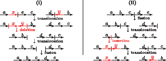
\end{document}-adjacencies of genome B can be first inserted at once as a cluster in genome A and later split with optimal DCJ operations, as we can see in Figure 3.
(i) An optimal scenario sorting \documentclass{aastex}\usepackage{amsbsy}\usepackage{amsfonts}\usepackage{amssymb}\usepackage{bm}\usepackage{mathrsfs}\usepackage{pifont}\usepackage{stmaryrd}\usepackage{textcomp}\usepackage{portland, xspace}\usepackage{amsmath, amsxtra}\pagestyle{empty}\DeclareMathSizes{10}{9}{7}{6}\begin{document}
$$\{ \circ axec \circ, \circ d \overline{y}b \circ \} \ {\rm into} \ \{ \circ abcde \circ \}$$
\end{document}. The first operation (translocation) accumulates x and y, so that they can be deleted at once. (ii) Conversely, while sorting \documentclass{aastex}\usepackage{amsbsy}\usepackage{amsfonts}\usepackage{amssymb}\usepackage{bm}\usepackage{mathrsfs}\usepackage{pifont}\usepackage{stmaryrd}\usepackage{textcomp}\usepackage{portland, xspace}\usepackage{amsmath, amsxtra}\pagestyle{empty}\DeclareMathSizes{10}{9}{7}{6}\begin{document}
$$\{ \circ abcde \circ \} \ {\rm into} \ \{ \circ axec \circ, \circ d \overline{y}b \circ \}$$
\end{document}, we can insert a cluster at once and later split it with a translocation.
Given a component C of AG(A, B), we can obtain a string ℓ(C) by the concatenation of the labels of the \documentclass{aastex}\usepackage{amsbsy}\usepackage{amsfonts}\usepackage{amssymb}\usepackage{bm}\usepackage{mathrsfs}\usepackage{pifont}\usepackage{stmaryrd}\usepackage{textcomp}\usepackage{portland, xspace}\usepackage{amsmath, amsxtra}\pagestyle{empty}\DeclareMathSizes{10}{9}{7}{6}\begin{document}
$${\cal G}$$
\end{document}-adjacencies of C in the order in which they appear. Cycles, AA-paths and BB-paths can be read in any direction, but AB-paths should always be read from A to B. If C is a cycle and has labels in both genomes A and B, we should start to read in a labeled \documentclass{aastex}\usepackage{amsbsy}\usepackage{amsfonts}\usepackage{amssymb}\usepackage{bm}\usepackage{mathrsfs}\usepackage{pifont}\usepackage{stmaryrd}\usepackage{textcomp}\usepackage{portland, xspace}\usepackage{amsmath, amsxtra}\pagestyle{empty}\DeclareMathSizes{10}{9}{7}{6}\begin{document}
$${\cal G}$$
\end{document}-adjacency v of A, such that the first labeled vertex before v is a \documentclass{aastex}\usepackage{amsbsy}\usepackage{amsfonts}\usepackage{amssymb}\usepackage{bm}\usepackage{mathrsfs}\usepackage{pifont}\usepackage{stmaryrd}\usepackage{textcomp}\usepackage{portland, xspace}\usepackage{amsmath, amsxtra}\pagestyle{empty}\DeclareMathSizes{10}{9}{7}{6}\begin{document}
$${\cal G}$$
\end{document}-adjacency in B; otherwise C has labels in at most one genome and we can start anywhere. Each maximal substring of ℓ(C) composed only of markers in \documentclass{aastex}\usepackage{amsbsy}\usepackage{amsfonts}\usepackage{amssymb}\usepackage{bm}\usepackage{mathrsfs}\usepackage{pifont}\usepackage{stmaryrd}\usepackage{textcomp}\usepackage{portland, xspace}\usepackage{amsmath, amsxtra}\pagestyle{empty}\DeclareMathSizes{10}{9}{7}{6}\begin{document}
$${\cal A}$$
\end{document} (respectively in \documentclass{aastex}\usepackage{amsbsy}\usepackage{amsfonts}\usepackage{amssymb}\usepackage{bm}\usepackage{mathrsfs}\usepackage{pifont}\usepackage{stmaryrd}\usepackage{textcomp}\usepackage{portland, xspace}\usepackage{amsmath, amsxtra}\pagestyle{empty}\DeclareMathSizes{10}{9}{7}{6}\begin{document}
$${\cal B}$$
\end{document}) is called an \documentclass{aastex}\usepackage{amsbsy}\usepackage{amsfonts}\usepackage{amssymb}\usepackage{bm}\usepackage{mathrsfs}\usepackage{pifont}\usepackage{stmaryrd}\usepackage{textcomp}\usepackage{portland, xspace}\usepackage{amsmath, amsxtra}\pagestyle{empty}\DeclareMathSizes{10}{9}{7}{6}\begin{document}
$${\cal A}$$
\end{document}-run (respectively a \documentclass{aastex}\usepackage{amsbsy}\usepackage{amsfonts}\usepackage{amssymb}\usepackage{bm}\usepackage{mathrsfs}\usepackage{pifont}\usepackage{stmaryrd}\usepackage{textcomp}\usepackage{portland, xspace}\usepackage{amsmath, amsxtra}\pagestyle{empty}\DeclareMathSizes{10}{9}{7}{6}\begin{document}
$${\cal B}$$
\end{document}-run). Each \documentclass{aastex}\usepackage{amsbsy}\usepackage{amsfonts}\usepackage{amssymb}\usepackage{bm}\usepackage{mathrsfs}\usepackage{pifont}\usepackage{stmaryrd}\usepackage{textcomp}\usepackage{portland, xspace}\usepackage{amsmath, amsxtra}\pagestyle{empty}\DeclareMathSizes{10}{9}{7}{6}\begin{document}
$${\cal A}$$
\end{document}-run or \documentclass{aastex}\usepackage{amsbsy}\usepackage{amsfonts}\usepackage{amssymb}\usepackage{bm}\usepackage{mathrsfs}\usepackage{pifont}\usepackage{stmaryrd}\usepackage{textcomp}\usepackage{portland, xspace}\usepackage{amsmath, amsxtra}\pagestyle{empty}\DeclareMathSizes{10}{9}{7}{6}\begin{document}
$${\cal B}$$
\end{document}-run can be simply called run. A component composed only of clean \documentclass{aastex}\usepackage{amsbsy}\usepackage{amsfonts}\usepackage{amssymb}\usepackage{bm}\usepackage{mathrsfs}\usepackage{pifont}\usepackage{stmaryrd}\usepackage{textcomp}\usepackage{portland, xspace}\usepackage{amsmath, amsxtra}\pagestyle{empty}\DeclareMathSizes{10}{9}{7}{6}\begin{document}
$${\cal G}$$
\end{document}-adjacencies has no run and is said to be clean, otherwise the component is labeled. We denote by Λ(C) the number of runs in a component C. A path can have any number of runs, while a cycle has zero, one, or an even number of runs. Figure 4 shows an AB-path with three runs.
An AB-path with three runs. Only the labels of the \documentclass{aastex}\usepackage{amsbsy}\usepackage{amsfonts}\usepackage{amssymb}\usepackage{bm}\usepackage{mathrsfs}\usepackage{pifont}\usepackage{stmaryrd}\usepackage{textcomp}\usepackage{portland, xspace}\usepackage{amsmath, amsxtra}\pagestyle{empty}\DeclareMathSizes{10}{9}{7}{6}\begin{document}
$${\cal G}$$
\end{document}-adjacencies are represented.
Proposition 1
If γ1γ2is a clean\documentclass{aastex}\usepackage{amsbsy}\usepackage{amsfonts}\usepackage{amssymb}\usepackage{bm}\usepackage{mathrsfs}\usepackage{pifont}\usepackage{stmaryrd}\usepackage{textcomp}\usepackage{portland, xspace}\usepackage{amsmath, amsxtra}\pagestyle{empty}\DeclareMathSizes{10}{9}{7}{6}\begin{document}
$${\cal G}$$
\end{document}-adjacency in a DCJ-unsorted component C of AG(A, B), such that neither γ1nor γ2are telomeres, then it is always possible to extract a clean cycle from C with an optimal DCJ operation.
Proof
If γ1γ2 is in \documentclass{aastex}\usepackage{amsbsy}\usepackage{amsfonts}\usepackage{amssymb}\usepackage{bm}\usepackage{mathrsfs}\usepackage{pifont}\usepackage{stmaryrd}\usepackage{textcomp}\usepackage{portland, xspace}\usepackage{amsmath, amsxtra}\pagestyle{empty}\DeclareMathSizes{10}{9}{7}{6}\begin{document}
$$V_{\cal G} (B)$$
\end{document}, we apply a DCJ on the two vertices γ1ℓ1γ3 and γ2ℓ2γ4 of \documentclass{aastex}\usepackage{amsbsy}\usepackage{amsfonts}\usepackage{amssymb}\usepackage{bm}\usepackage{mathrsfs}\usepackage{pifont}\usepackage{stmaryrd}\usepackage{textcomp}\usepackage{portland, xspace}\usepackage{amsmath, amsxtra}\pagestyle{empty}\DeclareMathSizes{10}{9}{7}{6}\begin{document}
$$V_{\cal G} (A)$$
\end{document} that are neighbors of γ1γ2, creating the two new vertices \documentclass{aastex}\usepackage{amsbsy}\usepackage{amsfonts}\usepackage{amssymb}\usepackage{bm}\usepackage{mathrsfs}\usepackage{pifont}\usepackage{stmaryrd}\usepackage{textcomp}\usepackage{portland, xspace}\usepackage{amsmath, amsxtra}\pagestyle{empty}\DeclareMathSizes{10}{9}{7}{6}\begin{document}
$$\gamma_3 \overline{\ell}_1 \ell_2 \gamma_4$$
\end{document} and γ1γ2. Observe that the vertex γ1γ2 in \documentclass{aastex}\usepackage{amsbsy}\usepackage{amsfonts}\usepackage{amssymb}\usepackage{bm}\usepackage{mathrsfs}\usepackage{pifont}\usepackage{stmaryrd}\usepackage{textcomp}\usepackage{portland, xspace}\usepackage{amsmath, amsxtra}\pagestyle{empty}\DeclareMathSizes{10}{9}{7}{6}\begin{document}
$$V_{\cal G} (B)$$
\end{document} and the new vertex γ1γ2 in \documentclass{aastex}\usepackage{amsbsy}\usepackage{amsfonts}\usepackage{amssymb}\usepackage{bm}\usepackage{mathrsfs}\usepackage{pifont}\usepackage{stmaryrd}\usepackage{textcomp}\usepackage{portland, xspace}\usepackage{amsmath, amsxtra}\pagestyle{empty}\DeclareMathSizes{10}{9}{7}{6}\begin{document}
$$V_{\cal G} (A)$$
\end{document} are extracted into a clean cycle. Analogously, if γ1γ2 is in \documentclass{aastex}\usepackage{amsbsy}\usepackage{amsfonts}\usepackage{amssymb}\usepackage{bm}\usepackage{mathrsfs}\usepackage{pifont}\usepackage{stmaryrd}\usepackage{textcomp}\usepackage{portland, xspace}\usepackage{amsmath, amsxtra}\pagestyle{empty}\DeclareMathSizes{10}{9}{7}{6}\begin{document}
$$V_{\cal G} (A)$$
\end{document}, we do the same procedure using the two vertices of \documentclass{aastex}\usepackage{amsbsy}\usepackage{amsfonts}\usepackage{amssymb}\usepackage{bm}\usepackage{mathrsfs}\usepackage{pifont}\usepackage{stmaryrd}\usepackage{textcomp}\usepackage{portland, xspace}\usepackage{amsmath, amsxtra}\pagestyle{empty}\DeclareMathSizes{10}{9}{7}{6}\begin{document}
$$V_{\cal G} (B)$$
\end{document} that are neighbors of γ1γ2. ▪
Proposition 2
A run can be entirely accumulated in the label of one single\documentclass{aastex}\usepackage{amsbsy}\usepackage{amsfonts}\usepackage{amssymb}\usepackage{bm}\usepackage{mathrsfs}\usepackage{pifont}\usepackage{stmaryrd}\usepackage{textcomp}\usepackage{portland, xspace}\usepackage{amsmath, amsxtra}\pagestyle{empty}\DeclareMathSizes{10}{9}{7}{6}\begin{document}
$${\cal G}$$
\end{document}-adjacency with optimal DCJ operations.
Proof
A run that is not yet accumulated is distributed over two or more \documentclass{aastex}\usepackage{amsbsy}\usepackage{amsfonts}\usepackage{amssymb}\usepackage{bm}\usepackage{mathrsfs}\usepackage{pifont}\usepackage{stmaryrd}\usepackage{textcomp}\usepackage{portland, xspace}\usepackage{amsmath, amsxtra}\pagestyle{empty}\DeclareMathSizes{10}{9}{7}{6}\begin{document}
$${\cal G}$$
\end{document}-adjacencies in one genome. The \documentclass{aastex}\usepackage{amsbsy}\usepackage{amsfonts}\usepackage{amssymb}\usepackage{bm}\usepackage{mathrsfs}\usepackage{pifont}\usepackage{stmaryrd}\usepackage{textcomp}\usepackage{portland, xspace}\usepackage{amsmath, amsxtra}\pagestyle{empty}\DeclareMathSizes{10}{9}{7}{6}\begin{document}
$${\cal G}$$
\end{document}-adjacencies in the other genome within the run are clean. We can thus apply optimal DCJs that extract clean cycles (Proposition 1) and accumulate the entire run in the label of one \documentclass{aastex}\usepackage{amsbsy}\usepackage{amsfonts}\usepackage{amssymb}\usepackage{bm}\usepackage{mathrsfs}\usepackage{pifont}\usepackage{stmaryrd}\usepackage{textcomp}\usepackage{portland, xspace}\usepackage{amsmath, amsxtra}\pagestyle{empty}\DeclareMathSizes{10}{9}{7}{6}\begin{document}
$${\cal G}$$
\end{document}-adjacency. ▪
Proposition 2 immediately gives an upper bound for the distance:
Lemma 1
Given two genomes A and B without duplicated markers, we have\documentclass{aastex}\usepackage{amsbsy}\usepackage{amsfonts}\usepackage{amssymb}\usepackage{bm}\usepackage{mathrsfs}\usepackage{pifont}\usepackage{stmaryrd}\usepackage{textcomp}\usepackage{portland, xspace}\usepackage{amsmath, amsxtra}\pagestyle{empty}\DeclareMathSizes{10}{9}{7}{6}\begin{document}
\begin{align*}
d_{DCJ}^{id} (A, B) \leq d_{DCJ} (A, B) + \sum_{C \in AG (A, B)} \Lambda (C).
\end{align*}
\end{document}
For some instances of A and B, the upper bound of Lemma 1 gives the exact number of steps required to sort A into B. However, since two runs can be merged together with a DCJ operation, the DCJ-indel distance is often smaller than this upper bound. Given a DCJ operation ρ, let Λ0 and Λ1 be, respectively, the number of runs in AG(A, B) before and after ρ. We define ΔΛ(ρ) = Λ1 − Λ0.
Proposition 3
Given any DCJ operation ρ, we have ΔΛ(ρ) ≥ −2.
Proof
If ρ cuts between an \documentclass{aastex}\usepackage{amsbsy}\usepackage{amsfonts}\usepackage{amssymb}\usepackage{bm}\usepackage{mathrsfs}\usepackage{pifont}\usepackage{stmaryrd}\usepackage{textcomp}\usepackage{portland, xspace}\usepackage{amsmath, amsxtra}\pagestyle{empty}\DeclareMathSizes{10}{9}{7}{6}\begin{document}
$${\cal A}$$
\end{document}-run r1 and a \documentclass{aastex}\usepackage{amsbsy}\usepackage{amsfonts}\usepackage{amssymb}\usepackage{bm}\usepackage{mathrsfs}\usepackage{pifont}\usepackage{stmaryrd}\usepackage{textcomp}\usepackage{portland, xspace}\usepackage{amsmath, amsxtra}\pagestyle{empty}\DeclareMathSizes{10}{9}{7}{6}\begin{document}
$${\cal B}$$
\end{document}-run r2 and between an \documentclass{aastex}\usepackage{amsbsy}\usepackage{amsfonts}\usepackage{amssymb}\usepackage{bm}\usepackage{mathrsfs}\usepackage{pifont}\usepackage{stmaryrd}\usepackage{textcomp}\usepackage{portland, xspace}\usepackage{amsmath, amsxtra}\pagestyle{empty}\DeclareMathSizes{10}{9}{7}{6}\begin{document}
$${\cal A}$$
\end{document}-run r3 and a \documentclass{aastex}\usepackage{amsbsy}\usepackage{amsfonts}\usepackage{amssymb}\usepackage{bm}\usepackage{mathrsfs}\usepackage{pifont}\usepackage{stmaryrd}\usepackage{textcomp}\usepackage{portland, xspace}\usepackage{amsmath, amsxtra}\pagestyle{empty}\DeclareMathSizes{10}{9}{7}{6}\begin{document}
$${\cal B}$$
\end{document}-run r4, with r1 ≠ r3 and r2 ≠ r4, and joins r1 with r3 and r2 with r4, then ΔΛ(ρ) = −2. As a DCJ has at most two cuts and two joins, it is not possible to do better, that is ΔΛ(ρ) ≥ −2. ▪
In order to obtain the exact formula for the DCJ-indel distance, we will first analyze the components of the adjacency graph separately. Given two genomes A and B and a component \documentclass{aastex}\usepackage{amsbsy}\usepackage{amsfonts}\usepackage{amssymb}\usepackage{bm}\usepackage{mathrsfs}\usepackage{pifont}\usepackage{stmaryrd}\usepackage{textcomp}\usepackage{portland, xspace}\usepackage{amsmath, amsxtra}\pagestyle{empty}\DeclareMathSizes{10}{9}{7}{6}\begin{document}
$$C \in AG (A, B)$$
\end{document}, we denote by dDCJ(C) the minimum number of DCJ operations required to do a separate DCJ-sorting in C, applying DCJs only on vertices of C (or vertices that result from DCJs applied on vertices that were in C). From Braga and Stoye (2010), we know that it is possible to do a separate DCJ-sorting using only optimal DCJs in any component of AG(A, B), or, in other words, \documentclass{aastex}\usepackage{amsbsy}\usepackage{amsfonts}\usepackage{amssymb}\usepackage{bm}\usepackage{mathrsfs}\usepackage{pifont}\usepackage{stmaryrd}\usepackage{textcomp}\usepackage{portland, xspace}\usepackage{amsmath, amsxtra}\pagestyle{empty}\DeclareMathSizes{10}{9}{7}{6}\begin{document}
$$d_{DCJ} (A, B) = \sum \nolimits_{C \in AG (A, B)}d_{DCJ} (C)$$
\end{document}.
We then define the indel-potential of a component C, denoted by λ(C), as the minimum number of runs that we can obtain doing a separate DCJ-sorting in C with optimal DCJ operations. The indel-potential of a component C can be computed with a simple formula that depends only on the number of runs in C:
Proposition 4
Given a component C in AG(A,B), the indel-potential of C is given by\documentclass{aastex}\usepackage{amsbsy}\usepackage{amsfonts}\usepackage{amssymb}\usepackage{bm}\usepackage{mathrsfs}\usepackage{pifont}\usepackage{stmaryrd}\usepackage{textcomp}\usepackage{portland, xspace}\usepackage{amsmath, amsxtra}\pagestyle{empty}\DeclareMathSizes{10}{9}{7}{6}\begin{document}
$$\lambda (C) = \left\lceil \frac {\Lambda(C) + 1} {2} \right\rceil,$$
\end{document}if Λ(C) ≥ 1. Otherwise λ(C) = 0.
Proof
The proof is by induction on i = Λ(C) and the hypothesis is \documentclass{aastex}\usepackage{amsbsy}\usepackage{amsfonts}\usepackage{amssymb}\usepackage{bm}\usepackage{mathrsfs}\usepackage{pifont}\usepackage{stmaryrd}\usepackage{textcomp}\usepackage{portland, xspace}\usepackage{amsmath, amsxtra}\pagestyle{empty}\DeclareMathSizes{10}{9}{7}{6}\begin{document}
$$T (i) = \left\lceil \frac {i + 1} {2} \right\rceil$$
\end{document}. A labeled DCJ-sorted component can have one or two runs, thus we need two base cases, T(1) = 1 and T(2) = 2. These cases can be easily verified. More intricate is the inductive step, for i ≥ 3.
If i = 3, the best we can do is to merge the first and the last runs with an optimal DCJ, obtaining a cycle with two runs. This gives \documentclass{aastex}\usepackage{amsbsy}\usepackage{amsfonts}\usepackage{amssymb}\usepackage{bm}\usepackage{mathrsfs}\usepackage{pifont}\usepackage{stmaryrd}\usepackage{textcomp}\usepackage{portland, xspace}\usepackage{amsmath, amsxtra}\pagestyle{empty}\DeclareMathSizes{10}{9}{7}{6}\begin{document}
$$T (3) = T (2) = \left\lceil \frac {2 + 1} {2} \right\rceil = \left\lceil \frac {3 + 1} {2} \right\rceil$$
\end{document}. If i = 4, any optimal DCJ merging runs would split the original component C into a cycle with two runs and another component with only one run. This gives \documentclass{aastex}\usepackage{amsbsy}\usepackage{amsfonts}\usepackage{amssymb}\usepackage{bm}\usepackage{mathrsfs}\usepackage{pifont}\usepackage{stmaryrd}\usepackage{textcomp}\usepackage{portland, xspace}\usepackage{amsmath, amsxtra}\pagestyle{empty}\DeclareMathSizes{10}{9}{7}{6}\begin{document}
$$T (4) = T (2) + T (1) = 3 = \left\lceil \frac {4 + 1} {2} \right\rceil$$
\end{document}.
If i ≥ 5, the best we can do is to use a DCJ with ΔΛ = −2, that extracts three consecutive runs into a cycle of two runs and leaves the other component with i − 4 runs. We then have \documentclass{aastex}\usepackage{amsbsy}\usepackage{amsfonts}\usepackage{amssymb}\usepackage{bm}\usepackage{mathrsfs}\usepackage{pifont}\usepackage{stmaryrd}\usepackage{textcomp}\usepackage{portland, xspace}\usepackage{amsmath, amsxtra}\pagestyle{empty}\DeclareMathSizes{10}{9}{7}{6}\begin{document}
$$T (i) = T (2) + T (i - 4) = 2 + \left\lceil \frac {i - 4 + 1} {2} \right\rceil = \left\lceil \frac {i - 4 + 1 + 4} {2} \right\rceil = \left\lceil \frac {i + 1} {2} \right\rceil$$
\end{document}. ▪
If λ0 and λ1 are, respectively, the sum of the indel-potentials for the components of the adjacency graph before and after a DCJ operation ρ, we define Δλ(ρ) = λ1 − λ0. By the definition of λ, any optimal DCJ ρ acting on a single component has Δλ(ρ) ≥ 0. However, considering the case in which only one component is affected by ρ, we still need to investigate Δλ(ρ) when ρ is neutral or counter-optimal.
Proposition 5
Given a DCJ operation ρ acting on a single component, we have Δλ(ρ) ≥ 0, if ρ is counter-optimal, and Δλ(ρ) ≥ −1, if ρ is neutral.
Proof
The linearization of a cycle is the only counter-optimal DCJ that acts on a single component. This can decrease neither Λ, nor λ. Moreover, when Λ ≤ 2, it is not possible to decrease the indel-potential with any DCJ. When the component has Λ = 3, the best we can get with a neutral ρ is ΔΛ(ρ) = −1. This gives \documentclass{aastex}\usepackage{amsbsy}\usepackage{amsfonts}\usepackage{amssymb}\usepackage{bm}\usepackage{mathrsfs}\usepackage{pifont}\usepackage{stmaryrd}\usepackage{textcomp}\usepackage{portland, xspace}\usepackage{amsmath, amsxtra}\pagestyle{empty}\DeclareMathSizes{10}{9}{7}{6}\begin{document}
$$\lambda_1 = \left\lceil \frac {(3 - 1) + 1} {2} \right\rceil = \left\lceil \frac {3} {2} \right\rceil = \left\lceil \frac {3 + 1} {2} \right\rceil = \lambda_0$$
\end{document}, that is, Δλ(ρ) = 0. And when the component has Λ ≥ 4, we can get ΔΛ(ρ) = −2 with a neutral ρ, resulting in \documentclass{aastex}\usepackage{amsbsy}\usepackage{amsfonts}\usepackage{amssymb}\usepackage{bm}\usepackage{mathrsfs}\usepackage{pifont}\usepackage{stmaryrd}\usepackage{textcomp}\usepackage{portland, xspace}\usepackage{amsmath, amsxtra}\pagestyle{empty}\DeclareMathSizes{10}{9}{7}{6}\begin{document}
$$\lambda_1 = \left\lceil \frac {(\Lambda (C) - 2) + 1} {2} \right\rceil = \left\lceil \frac {\Lambda (C) + 1} {2} \right\rceil - 1 = \lambda_0 - 1$$
\end{document}, that is, Δλ(ρ) = −1. ▪
We denote by \documentclass{aastex}\usepackage{amsbsy}\usepackage{amsfonts}\usepackage{amssymb}\usepackage{bm}\usepackage{mathrsfs}\usepackage{pifont}\usepackage{stmaryrd}\usepackage{textcomp}\usepackage{portland, xspace}\usepackage{amsmath, amsxtra}\pagestyle{empty}\DeclareMathSizes{10}{9}{7}{6}\begin{document}
$$d_{DCJ}^{id} (C)$$
\end{document} the minimum number of DCJ and indel operations required to sort separately a component C of AG(A, B).
Proposition 6
If C is a component of AG(A, B), then we have\documentclass{aastex}\usepackage{amsbsy}\usepackage{amsfonts}\usepackage{amssymb}\usepackage{bm}\usepackage{mathrsfs}\usepackage{pifont}\usepackage{stmaryrd}\usepackage{textcomp}\usepackage{portland, xspace}\usepackage{amsmath, amsxtra}\pagestyle{empty}\DeclareMathSizes{10}{9}{7}{6}\begin{document}
$$d^{id}_{DCJ} (C) = d_{DCJ} (C) + \lambda (C)$$
\end{document}.
Proof
By the definition of λ, the best we can do with optimal DCJs is dDCJ(C) + λ(C). From Proposition 5, we know that Δλ(ρ) ≥ 0 if ρ is a counter-optimal DCJ, thus we can only get longer sorting scenarios if we use such operations. We also know that Δλ(ρ) ≥ −1 if ρ is neutral, and, since this kind of operation increases the sorting scenario by one with respect to the scenario with only optimal DCJs, this gives at least dDCJ(C) + λ(C). ▪
Proposition 6 gives a new upper bound for the DCJ-indel distance:
Lemma 2
Given two genomes A and B without duplicated markers, we have\documentclass{aastex}\usepackage{amsbsy}\usepackage{amsfonts}\usepackage{amssymb}\usepackage{bm}\usepackage{mathrsfs}\usepackage{pifont}\usepackage{stmaryrd}\usepackage{textcomp}\usepackage{portland, xspace}\usepackage{amsmath, amsxtra}\pagestyle{empty}\DeclareMathSizes{10}{9}{7}{6}\begin{document}
\begin{align*}
d_{DCJ}^{id} (A, B) \leq d_{DCJ} (A, B) + \sum_{C \in AG (A,
B)} \lambda (C).
\end{align*}
\end{document}
Proof
We can sort the components separately with \documentclass{aastex}\usepackage{amsbsy}\usepackage{amsfonts}\usepackage{amssymb}\usepackage{bm}\usepackage{mathrsfs}\usepackage{pifont}\usepackage{stmaryrd}\usepackage{textcomp}\usepackage{portland, xspace}\usepackage{amsmath, amsxtra}\pagestyle{empty}\DeclareMathSizes{10}{9}{7}{6}\begin{document}
$$\sum \nolimits_{C \in AG (A, B)}d_{DCJ}^{id} (C)$$
\end{document} steps, which corresponds exactly to \documentclass{aastex}\usepackage{amsbsy}\usepackage{amsfonts}\usepackage{amssymb}\usepackage{bm}\usepackage{mathrsfs}\usepackage{pifont}\usepackage{stmaryrd}\usepackage{textcomp}\usepackage{portland, xspace}\usepackage{amsmath, amsxtra}\pagestyle{empty}\DeclareMathSizes{10}{9}{7}{6}\begin{document}
$$d_{DCJ} (A, B) + \sum \nolimits_{C \in AG (A, B)} \lambda (C)$$
\end{document}. ▪
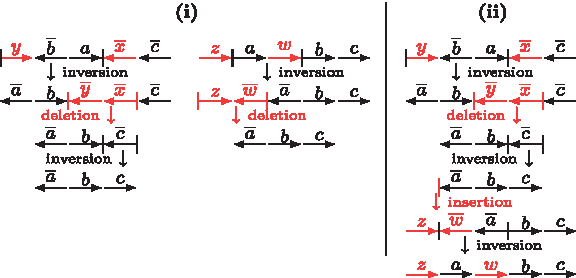
Since λ(C) ≤ Λ(C), the upper bound given by Lemma 2 is tighter than the one given by Lemma 1, but can still be improved. Observe that a parsimonious scenario may not simply consist of optimal DCJ operations, insertions and deletions. Sometimes a neutral DCJ can lead to a shorter sequence of operations sorting one genome into another one, as we can see in Figure 5.
An optimal scenario sorting \documentclass{aastex}\usepackage{amsbsy}\usepackage{amsfonts}\usepackage{amssymb}\usepackage{bm}\usepackage{mathrsfs}\usepackage{pifont}\usepackage{stmaryrd}\usepackage{textcomp}\usepackage{portland, xspace}\usepackage{amsmath, amsxtra}\pagestyle{empty}\DeclareMathSizes{10}{9}{7}{6}\begin{document}
$$\{ \circ ab \circ, \circ cd \circ \} \ {\rm into} \ \{ \circ a \circ, \circ b \circ, \circ c \circ, \circ d \circ \}$$
\end{document}(i) and two different scenarios sorting \documentclass{aastex}\usepackage{amsbsy}\usepackage{amsfonts}\usepackage{amssymb}\usepackage{bm}\usepackage{mathrsfs}\usepackage{pifont}\usepackage{stmaryrd}\usepackage{textcomp}\usepackage{portland, xspace}\usepackage{amsmath, amsxtra}\pagestyle{empty}\DeclareMathSizes{10}{9}{7}{6}\begin{document}
$$\{ \circ axb \circ, \circ cyd \circ \} \ {\rm into} \ \{ \circ a \circ, \circ ub \circ, \circ c \circ, \circ vd \circ \} $$
\end{document}. In (ii) in addition to the two optimal DCJ operations (fissions) from (i) we have two insertions and two deletions, using six steps. In (iii), we first use a neutral DCJ operation (translocation) that allows us to do only one deletion and one insertion, achieving a total of five steps.
4. The DCJ-Indel Distance
A DCJ operation ρ that acts on two components is called a recombination and can have Δλ(ρ) = −2. The two components on which the cuts are applied are called sources and the components obtained after the joinings are called resultants of the recombination.
Proposition 7
Given any recombination ρ, we have Δλ(ρ) ≥ −2.
Proof
Only the recombinations that decrease or do not change the number of runs (ΔΛ ≤ 0) have to be analyzed (we can not have Δλ ≤ −1 if the number of runs increases). First consider the recombination of two paths with i and j runs, respectively, that results in two new paths with i′ and j′ runs. Observe that the best we can have is when i and j are even, i′ and j′ are odd and ΔΛ = −2, that gives: \documentclass{aastex}\usepackage{amsbsy}\usepackage{amsfonts}\usepackage{amssymb}\usepackage{bm}\usepackage{mathrsfs}\usepackage{pifont}\usepackage{stmaryrd}\usepackage{textcomp}\usepackage{portland, xspace}\usepackage{amsmath, amsxtra}\pagestyle{empty}\DeclareMathSizes{10}{9}{7}{6}\begin{document}
$$\lambda_1 = \left\lceil \frac {i^ {\prime} + 1} {2} \right\rceil + \left\lceil \frac {j^ {\prime} + 1} {2} \right\rceil = \frac {i^ {\prime} + j^ {\prime} + 2} {2} = \frac {i + j} {2} = \frac {i} {2} + \frac {j} {2} = \left\lceil \frac {i + 1} {2} \right\rceil - 1 + \left\lceil \frac {j + 1} {2} \right\rceil - 1 = \lambda_0 - 2$$
\end{document}. The analysis of recombinations involving cycles is analogous. ▪
Given a recombination ρ, let Δdcj(ρ) be respectively 0, +1 and +2 depending whether ρ is optimal, neutral or counter-optimal. Any recombination applied to a vertex of an AA-path and a vertex of a BB-path is optimal (Braga and Stoye, 2010). A recombination applied to vertices of two different AB-paths can be either neutral, when the result is also a pair of AB-paths, or counter-optimal, when the result is a pair composed of an AA-path and a BB-path. All other types of path recombinations are neutral. In addition, all recombinations involving at least one cycle are counter-optimal. We define Δd(ρ) = Δdcj(ρ) + Δλ(ρ). Any counter-optimal recombination has Δd ≥ 0, thus only path recombinations can have Δd ≤ −1.
Let \documentclass{aastex}\usepackage{amsbsy}\usepackage{amsfonts}\usepackage{amssymb}\usepackage{bm}\usepackage{mathrsfs}\usepackage{pifont}\usepackage{stmaryrd}\usepackage{textcomp}\usepackage{portland, xspace}\usepackage{amsmath, amsxtra}\pagestyle{empty}\DeclareMathSizes{10}{9}{7}{6}\begin{document}
$${\cal A}$$
\end{document} (respectively \documentclass{aastex}\usepackage{amsbsy}\usepackage{amsfonts}\usepackage{amssymb}\usepackage{bm}\usepackage{mathrsfs}\usepackage{pifont}\usepackage{stmaryrd}\usepackage{textcomp}\usepackage{portland, xspace}\usepackage{amsmath, amsxtra}\pagestyle{empty}\DeclareMathSizes{10}{9}{7}{6}\begin{document}
$${\cal B}$$
\end{document}) be a sequence with an odd (≥1) number of runs, starting and ending with an \documentclass{aastex}\usepackage{amsbsy}\usepackage{amsfonts}\usepackage{amssymb}\usepackage{bm}\usepackage{mathrsfs}\usepackage{pifont}\usepackage{stmaryrd}\usepackage{textcomp}\usepackage{portland, xspace}\usepackage{amsmath, amsxtra}\pagestyle{empty}\DeclareMathSizes{10}{9}{7}{6}\begin{document}
$${\cal A}$$
\end{document}-run (respectively \documentclass{aastex}\usepackage{amsbsy}\usepackage{amsfonts}\usepackage{amssymb}\usepackage{bm}\usepackage{mathrsfs}\usepackage{pifont}\usepackage{stmaryrd}\usepackage{textcomp}\usepackage{portland, xspace}\usepackage{amsmath, amsxtra}\pagestyle{empty}\DeclareMathSizes{10}{9}{7}{6}\begin{document}
$${\cal B}$$
\end{document}-run). We can then make any combination of \documentclass{aastex}\usepackage{amsbsy}\usepackage{amsfonts}\usepackage{amssymb}\usepackage{bm}\usepackage{mathrsfs}\usepackage{pifont}\usepackage{stmaryrd}\usepackage{textcomp}\usepackage{portland, xspace}\usepackage{amsmath, amsxtra}\pagestyle{empty}\DeclareMathSizes{10}{9}{7}{6}\begin{document}
$${\cal A} \ {\rm and} \ {\cal B}$$
\end{document}, such as \documentclass{aastex}\usepackage{amsbsy}\usepackage{amsfonts}\usepackage{amssymb}\usepackage{bm}\usepackage{mathrsfs}\usepackage{pifont}\usepackage{stmaryrd}\usepackage{textcomp}\usepackage{portland, xspace}\usepackage{amsmath, amsxtra}\pagestyle{empty}\DeclareMathSizes{10}{9}{7}{6}\begin{document}
$${\cal AB}$$
\end{document}, that is a sequence with an even (≥2) number of runs, starting with an \documentclass{aastex}\usepackage{amsbsy}\usepackage{amsfonts}\usepackage{amssymb}\usepackage{bm}\usepackage{mathrsfs}\usepackage{pifont}\usepackage{stmaryrd}\usepackage{textcomp}\usepackage{portland, xspace}\usepackage{amsmath, amsxtra}\pagestyle{empty}\DeclareMathSizes{10}{9}{7}{6}\begin{document}
$${\cal A}$$
\end{document}-run and ending with a \documentclass{aastex}\usepackage{amsbsy}\usepackage{amsfonts}\usepackage{amssymb}\usepackage{bm}\usepackage{mathrsfs}\usepackage{pifont}\usepackage{stmaryrd}\usepackage{textcomp}\usepackage{portland, xspace}\usepackage{amsmath, amsxtra}\pagestyle{empty}\DeclareMathSizes{10}{9}{7}{6}\begin{document}
$${\cal B}$$
\end{document}-run. An empty sequence (with no run) is represented by ɛ. Then each one of the notations \documentclass{aastex}\usepackage{amsbsy}\usepackage{amsfonts}\usepackage{amssymb}\usepackage{bm}\usepackage{mathrsfs}\usepackage{pifont}\usepackage{stmaryrd}\usepackage{textcomp}\usepackage{portland, xspace}\usepackage{amsmath, amsxtra}\pagestyle{empty}\DeclareMathSizes{10}{9}{7}{6}\begin{document}
$$AA_{\varepsilon}, AA_{\cal A}, AA_{\cal B}, AA_{\cal AB},
BB_{\varepsilon}, BB_{\cal A}, BB_{\cal B}, BB_{\cal AB},
AB_{\varepsilon}, AB_{\cal A}, AB_{\cal B}, AB_{\cal AB} \ {\rm
and} \ AB_{\cal BA}$$
\end{document} represents a particular type of path (AA, BB or AB) with a particular structure of runs \documentclass{aastex}\usepackage{amsbsy}\usepackage{amsfonts}\usepackage{amssymb}\usepackage{bm}\usepackage{mathrsfs}\usepackage{pifont}\usepackage{stmaryrd}\usepackage{textcomp}\usepackage{portland, xspace}\usepackage{amsmath, amsxtra}\pagestyle{empty}\DeclareMathSizes{10}{9}{7}{6}\begin{document}
$$(\varepsilon, {\cal A}, {\cal B}, {\cal AB} \ {\rm or} \ {\cal BA})$$
\end{document}. The complete set of path recombinations with Δd ≤ −1 is given in Table 1. In Table 2 we list recombinations with Δd = 0 that create at least one source of recombinations of Table 1. We denote by \documentclass{aastex}\usepackage{amsbsy}\usepackage{amsfonts}\usepackage{amssymb}\usepackage{bm}\usepackage{mathrsfs}\usepackage{pifont}\usepackage{stmaryrd}\usepackage{textcomp}\usepackage{portland, xspace}\usepackage{amsmath, amsxtra}\pagestyle{empty}\DeclareMathSizes{10}{9}{7}{6}\begin{document}
$$AB_\bullet$$
\end{document} an AB-path that can not be a source of a recombination in Tables 1 and 2, such as \documentclass{aastex}\usepackage{amsbsy}\usepackage{amsfonts}\usepackage{amssymb}\usepackage{bm}\usepackage{mathrsfs}\usepackage{pifont}\usepackage{stmaryrd}\usepackage{textcomp}\usepackage{portland, xspace}\usepackage{amsmath, amsxtra}\pagestyle{empty}\DeclareMathSizes{10}{9}{7}{6}\begin{document}
$$AB_{\varepsilon}, AB_{\cal A} \ and \ AB_{\cal B}$$
\end{document}.
Path Recombinations That Have Δd ≤ −1 and Allow the Best Reuse of the Resultants
The recombinations with Δd = 0 involving cycles or circular singletons cannot create new components that can be used as sources of recombinations listed in Tables 1 and 2.
Proof
A recombination ρ with Δd = 0 involving a cycle or a circular singleton C would integrate C to another component C′ without changing the type or the structure of runs in C′. Thus, if C′ is a source of a recombination in these tables after ρ, C′ was already the same type of source before ρ. And if C′ was not a source before ρ, C′ cannot become a source after ρ. ▪
With Proposition 8, we already have an exact formula to compute \documentclass{aastex}\usepackage{amsbsy}\usepackage{amsfonts}\usepackage{amssymb}\usepackage{bm}\usepackage{mathrsfs}\usepackage{pifont}\usepackage{stmaryrd}\usepackage{textcomp}\usepackage{portland, xspace}\usepackage{amsmath, amsxtra}\pagestyle{empty}\DeclareMathSizes{10}{9}{7}{6}\begin{document}
$$d^{id}_{DCJ}$$
\end{document} for a particular set of instances. Given a \documentclass{aastex}\usepackage{amsbsy}\usepackage{amsfonts}\usepackage{amssymb}\usepackage{bm}\usepackage{mathrsfs}\usepackage{pifont}\usepackage{stmaryrd}\usepackage{textcomp}\usepackage{portland, xspace}\usepackage{amsmath, amsxtra}\pagestyle{empty}\DeclareMathSizes{10}{9}{7}{6}\begin{document}
$${\cal G}$$
\end{document}-adjacency γℓ∘ of a genome A such that γ ≠ ∘, then γ is said to be a tail of a linear chromosome in A. Two genomes are co-tailed if their sets of tails are equal (this includes two genomes composed only of circular chromosomes).
Theorem 2
Given two co-tailed genomes A and B without duplicated markers, we have\documentclass{aastex}\usepackage{amsbsy}\usepackage{amsfonts}\usepackage{amssymb}\usepackage{bm}\usepackage{mathrsfs}\usepackage{pifont}\usepackage{stmaryrd}\usepackage{textcomp}\usepackage{portland, xspace}\usepackage{amsmath, amsxtra}\pagestyle{empty}\DeclareMathSizes{10}{9}{7}{6}\begin{document}
$$d^{id}_{DCJ} (A, B) = d_{DCJ} (A, B) + \sum \nolimits_{C \in AG (A, B)} \lambda (C)$$
\end{document}.
Proof
The graph AG(A, B) for co-tailed genomes A and B can have only cycles, singletons (that could be \documentclass{aastex}\usepackage{amsbsy}\usepackage{amsfonts}\usepackage{amssymb}\usepackage{bm}\usepackage{mathrsfs}\usepackage{pifont}\usepackage{stmaryrd}\usepackage{textcomp}\usepackage{portland, xspace}\usepackage{amsmath, amsxtra}\pagestyle{empty}\DeclareMathSizes{10}{9}{7}{6}\begin{document}
$$AA_{\cal A} \ {\rm and} \ BB_{\cal B}$$
\end{document}) and AB-paths of one edge (that could be \documentclass{aastex}\usepackage{amsbsy}\usepackage{amsfonts}\usepackage{amssymb}\usepackage{bm}\usepackage{mathrsfs}\usepackage{pifont}\usepackage{stmaryrd}\usepackage{textcomp}\usepackage{portland, xspace}\usepackage{amsmath, amsxtra}\pagestyle{empty}\DeclareMathSizes{10}{9}{7}{6}\begin{document}
$$AB_{\cal AB}$$
\end{document}, but never \documentclass{aastex}\usepackage{amsbsy}\usepackage{amsfonts}\usepackage{amssymb}\usepackage{bm}\usepackage{mathrsfs}\usepackage{pifont}\usepackage{stmaryrd}\usepackage{textcomp}\usepackage{portland, xspace}\usepackage{amsmath, amsxtra}\pagestyle{empty}\DeclareMathSizes{10}{9}{7}{6}\begin{document}
$$AB_{\cal BA}$$
\end{document}). Observe that with these paths no recombination with Δd ≤ −1 is possible. From Proposition 8, we also know that cycles cannot lead to recombinations with Δd ≤ −1. ▪
Now we continue the analysis for the general case. The two sources of a recombination can also be called partners. Looking at Table 1 we observe that all partners of \documentclass{aastex}\usepackage{amsbsy}\usepackage{amsfonts}\usepackage{amssymb}\usepackage{bm}\usepackage{mathrsfs}\usepackage{pifont}\usepackage{stmaryrd}\usepackage{textcomp}\usepackage{portland, xspace}\usepackage{amsmath, amsxtra}\pagestyle{empty}\DeclareMathSizes{10}{9}{7}{6}\begin{document}
$$AB_{\cal AB} \ {\rm and} \ AB_{\cal BA}$$
\end{document} paths are also partners of \documentclass{aastex}\usepackage{amsbsy}\usepackage{amsfonts}\usepackage{amssymb}\usepackage{bm}\usepackage{mathrsfs}\usepackage{pifont}\usepackage{stmaryrd}\usepackage{textcomp}\usepackage{portland, xspace}\usepackage{amsmath, amsxtra}\pagestyle{empty}\DeclareMathSizes{10}{9}{7}{6}\begin{document}
$$AA_{\cal AB} \ {\rm and} \ BB_{\cal AB}$$
\end{document} paths, all partners of \documentclass{aastex}\usepackage{amsbsy}\usepackage{amsfonts}\usepackage{amssymb}\usepackage{bm}\usepackage{mathrsfs}\usepackage{pifont}\usepackage{stmaryrd}\usepackage{textcomp}\usepackage{portland, xspace}\usepackage{amsmath, amsxtra}\pagestyle{empty}\DeclareMathSizes{10}{9}{7}{6}\begin{document}
$$AA_{\cal A} \ {\rm and} \ AA_{\cal B}$$
\end{document} paths are also partners of \documentclass{aastex}\usepackage{amsbsy}\usepackage{amsfonts}\usepackage{amssymb}\usepackage{bm}\usepackage{mathrsfs}\usepackage{pifont}\usepackage{stmaryrd}\usepackage{textcomp}\usepackage{portland, xspace}\usepackage{amsmath, amsxtra}\pagestyle{empty}\DeclareMathSizes{10}{9}{7}{6}\begin{document}
$$AA_{\cal AB}$$
\end{document} paths and all partners of \documentclass{aastex}\usepackage{amsbsy}\usepackage{amsfonts}\usepackage{amssymb}\usepackage{bm}\usepackage{mathrsfs}\usepackage{pifont}\usepackage{stmaryrd}\usepackage{textcomp}\usepackage{portland, xspace}\usepackage{amsmath, amsxtra}\pagestyle{empty}\DeclareMathSizes{10}{9}{7}{6}\begin{document}
$$BB_{\cal A} \ {\rm and} \ BB_{\cal B}$$
\end{document} paths are also partners of \documentclass{aastex}\usepackage{amsbsy}\usepackage{amsfonts}\usepackage{amssymb}\usepackage{bm}\usepackage{mathrsfs}\usepackage{pifont}\usepackage{stmaryrd}\usepackage{textcomp}\usepackage{portland, xspace}\usepackage{amsmath, amsxtra}\pagestyle{empty}\DeclareMathSizes{10}{9}{7}{6}\begin{document}
$$BB_{\cal AB}$$
\end{document} paths. Moreover, some resultants of recombinations in Tables 1 and 2 can be used in other recombinations. These observations allow the identification of recombination groups, as listed in Table 3.
All Recombination Groups (P, Q, T, and S) Obtained fromTable 1
Observe that the last four groups in T are subsets of groups in Q and the last ten groups in S are subsets of groups in T. The groups in M and N contain operations from Tables 1 and 2. All groups in N are subsets of the groups in M. The table is sorted in descending order with respect to the contribution of each path in the distance decrease (column scr).
The deductions shown in Table 3 can be computed with an approach that greedily maximizes the number of recombinations in P, Q, T, S, M and N in this order. The P part contains only one operation and is thus very simple. The same happens with Q, since the two groups in this part are mutually exclusive after applying P. The part T is only the application of all possible remaining groups of two operations with Δd = −2. Similarly, the part S is only the application of all possible remaining operations with Δd = −1. After S, the two groups in M are mutually exclusive and then the same happens to the six groups in N. Although some groups in T, S, M and N have some reusable resultants, those are actually never reused (if operations that are lower in the table use as sources resultants from higher operations, the sources of all referred operations would be previously consumed in operations that occupy even higher positions in the table). Due to this fact, the number of operations in P, Q, T, S, M and N depends only on the initial number of each type of component.
The results presented in this section give rise to the following theorem, which gives the exact formula for the DCJ-indel distance:
Theorem 3
Given two genomes A and B without duplicated markers, we have\documentclass{aastex}\usepackage{amsbsy}\usepackage{amsfonts}\usepackage{amssymb}\usepackage{bm}\usepackage{mathrsfs}\usepackage{pifont}\usepackage{stmaryrd}\usepackage{textcomp}\usepackage{portland, xspace}\usepackage{amsmath, amsxtra}\pagestyle{empty}\DeclareMathSizes{10}{9}{7}{6}\begin{document}
\begin{align*}
d^{id}_{DCJ} (A, B) = d_{DCJ} (A, B) + \sum_{C \in AG (A, B)}
\lambda (C) - 2P - 3Q - 2T - S - 2M - N,
\end{align*}
\end{document}
where the values P, Q, T, S, M and N are computed as described above.
Both AG(A, B) and dDCJ(A, B) can be computed in linear time (Bergeron et al., 2006). The runs can be obtained by a single walk through each component of AG(A, B), which is also linear. The algorithm to compute P, Q, T, S, M and N is a finite sequence of if and else statements, that depends only on the number of each type of labeled path in AG(A, B), thus the whole procedure takes linear time.
5. DCJ-Indel Sorting
One may have observed that the approach presented in the previous sections is bi-directional, allowing operations on both genomes A and B, in order to be able to accumulate labels in \documentclass{aastex}\usepackage{amsbsy}\usepackage{amsfonts}\usepackage{amssymb}\usepackage{bm}\usepackage{mathrsfs}\usepackage{pifont}\usepackage{stmaryrd}\usepackage{textcomp}\usepackage{portland, xspace}\usepackage{amsmath, amsxtra}\pagestyle{empty}\DeclareMathSizes{10}{9}{7}{6}\begin{document}
$${\cal G}$$
\end{document}-adjacencies of both genomes. As a result, we actually transform genomes A and B into an intermediate genome I. Regarding the operations applied on genome B, this can be seen as a backtracing to find the best moment to do a cluster insertion in genome A, as shown in Figure 6. Thus, with the operations that transform A and B into I, we can derive an optimal sequence of operations simply sorting genome A into B.
(i) Two sequences of lengths 3 and 2, sorting \documentclass{aastex}\usepackage{amsbsy}\usepackage{amsfonts}\usepackage{amssymb}\usepackage{bm}\usepackage{mathrsfs}\usepackage{pifont}\usepackage{stmaryrd}\usepackage{textcomp}\usepackage{portland, xspace}\usepackage{amsmath, amsxtra}\pagestyle{empty}\DeclareMathSizes{10}{9}{7}{6}\begin{document}
$$A = \{ \circ y \overline{b}a \overline{xc} \circ \} \ {\rm and} \ B = \{ \circ zawbc \circ \} \ {\rm into} \ I = \{ \circ \overline{a}bc \circ \}$$
\end{document}. (ii) A corresponding sequence of length 5 sorting A into B.
Given any DCJ or indel operation ρ = (X → Y), we define the inversion of ρ as ρ−1 = (Y → X). Observe that the inversion of a deletion is an insertion, and vice-versa. We can also extend this notation to a sequence of operations: given a sequence \documentclass{aastex}\usepackage{amsbsy}\usepackage{amsfonts}\usepackage{amssymb}\usepackage{bm}\usepackage{mathrsfs}\usepackage{pifont}\usepackage{stmaryrd}\usepackage{textcomp}\usepackage{portland, xspace}\usepackage{amsmath, amsxtra}\pagestyle{empty}\DeclareMathSizes{10}{9}{7}{6}\begin{document}
$$s = \rho_1 \rho_2 \ldots \rho_n$$
\end{document}, we have \documentclass{aastex}\usepackage{amsbsy}\usepackage{amsfonts}\usepackage{amssymb}\usepackage{bm}\usepackage{mathrsfs}\usepackage{pifont}\usepackage{stmaryrd}\usepackage{textcomp}\usepackage{portland, xspace}\usepackage{amsmath, amsxtra}\pagestyle{empty}\DeclareMathSizes{10}{9}{7}{6}\begin{document}
$$s^{- 1} = \rho_n^{- 1} \rho_{n - 1}^{- 1} \ldots \rho_2^{- 1} \rho_1^{- 1}$$
\end{document}.
Proposition 9
Given two genomes A and B, and a pair of sequences s1and s2composed of DCJ and indel operations acting on both genomes A and B, transforming respectively A and B into an intermediate genome I, such that\documentclass{aastex}\usepackage{amsbsy}\usepackage{amsfonts}\usepackage{amssymb}\usepackage{bm}\usepackage{mathrsfs}\usepackage{pifont}\usepackage{stmaryrd}\usepackage{textcomp}\usepackage{portland, xspace}\usepackage{amsmath, amsxtra}\pagestyle{empty}\DeclareMathSizes{10}{9}{7}{6}\begin{document}
$$\mid s_1 \mid + \mid s_2 \mid = d_{DCJ}^{id} (A, B)$$
\end{document}, then\documentclass{aastex}\usepackage{amsbsy}\usepackage{amsfonts}\usepackage{amssymb}\usepackage{bm}\usepackage{mathrsfs}\usepackage{pifont}\usepackage{stmaryrd}\usepackage{textcomp}\usepackage{portland, xspace}\usepackage{amsmath, amsxtra}\pagestyle{empty}\DeclareMathSizes{10}{9}{7}{6}\begin{document}
$$s_1s_2^{- 1}$$
\end{document}is an optimal sequence of DCJ and indel operations that transforms A into B.
Proof
First note that, since s1 sorts A into I and \documentclass{aastex}\usepackage{amsbsy}\usepackage{amsfonts}\usepackage{amssymb}\usepackage{bm}\usepackage{mathrsfs}\usepackage{pifont}\usepackage{stmaryrd}\usepackage{textcomp}\usepackage{portland, xspace}\usepackage{amsmath, amsxtra}\pagestyle{empty}\DeclareMathSizes{10}{9}{7}{6}\begin{document}
$$s_2^{- 1}$$
\end{document} sorts I into B, \documentclass{aastex}\usepackage{amsbsy}\usepackage{amsfonts}\usepackage{amssymb}\usepackage{bm}\usepackage{mathrsfs}\usepackage{pifont}\usepackage{stmaryrd}\usepackage{textcomp}\usepackage{portland, xspace}\usepackage{amsmath, amsxtra}\pagestyle{empty}\DeclareMathSizes{10}{9}{7}{6}\begin{document}
$$s_1 s_2^{- 1}$$
\end{document} sorts A into B. Furthermore, \documentclass{aastex}\usepackage{amsbsy}\usepackage{amsfonts}\usepackage{amssymb}\usepackage{bm}\usepackage{mathrsfs}\usepackage{pifont}\usepackage{stmaryrd}\usepackage{textcomp}\usepackage{portland, xspace}\usepackage{amsmath, amsxtra}\pagestyle{empty}\DeclareMathSizes{10}{9}{7}{6}\begin{document}
$$s_1 s_2^{- 1}$$
\end{document} has length \documentclass{aastex}\usepackage{amsbsy}\usepackage{amsfonts}\usepackage{amssymb}\usepackage{bm}\usepackage{mathrsfs}\usepackage{pifont}\usepackage{stmaryrd}\usepackage{textcomp}\usepackage{portland, xspace}\usepackage{amsmath, amsxtra}\pagestyle{empty}\DeclareMathSizes{10}{9}{7}{6}\begin{document}
$$d^{id}_{DCJ} (A, B)$$
\end{document} and is an optimal sorting sequence. Otherwise, there would exist a sorting sequence shorter than \documentclass{aastex}\usepackage{amsbsy}\usepackage{amsfonts}\usepackage{amssymb}\usepackage{bm}\usepackage{mathrsfs}\usepackage{pifont}\usepackage{stmaryrd}\usepackage{textcomp}\usepackage{portland, xspace}\usepackage{amsmath, amsxtra}\pagestyle{empty}\DeclareMathSizes{10}{9}{7}{6}\begin{document}
$$d^{id}_{DCJ} (A, B)$$
\end{document}, which is a contradiction. ▪
It is also interesting to observe that the space of solutions of the sorting problem contains scenarios with different compositions and, using the same number of steps, one could look for a scenario with more indels and less DCJ operations, or for a scenario with less indels and more DCJ operations. Figure 7 shows examples of two different approaches: one that minimizes the number of DCJs, and one that minimizes the number of indels. Both approaches will be presented in the following.
Two optimal scenarios sorting \documentclass{aastex}\usepackage{amsbsy}\usepackage{amsfonts}\usepackage{amssymb}\usepackage{bm}\usepackage{mathrsfs}\usepackage{pifont}\usepackage{stmaryrd}\usepackage{textcomp}\usepackage{portland, xspace}\usepackage{amsmath, amsxtra}\pagestyle{empty}\DeclareMathSizes{10}{9}{7}{6}\begin{document}
$$\{ \circ axec \circ, \circ d \overline{y}b \circ \} \ {\rm into} \ \{ \circ aubcdve \circ \}$$
\end{document}. (i) Minimizing DCJs gives three DCJs and three indels. (ii) Minimizing indels gives four DCJs and two indels.
5.1. Sorting with a minimum number of DCJ operations
First we will derive a sorting algorithm directly from the formula given in Theorem 3. In general lines, Algorithm 1 constructs incrementally two sequences of operations, s1 and s2, such that the operations in s1 are applied on A and the operations in s2 are applied on B (although we do not explicitly identify in the pseudo-code which operations are in s1 and which operations are in s2). As previously stated, an optimal sequence sorting A into B is given by \documentclass{aastex}\usepackage{amsbsy}\usepackage{amsfonts}\usepackage{amssymb}\usepackage{bm}\usepackage{mathrsfs}\usepackage{pifont}\usepackage{stmaryrd}\usepackage{textcomp}\usepackage{portland, xspace}\usepackage{amsmath, amsxtra}\pagestyle{empty}\DeclareMathSizes{10}{9}{7}{6}\begin{document}
$$s_1 s_2^{- 1}$$
\end{document}.
Sorting genome A into B with a minimum number of DCJs
1. Apply all P, Q, T, S, M and N-recombinations, in this order.
2. For each component \documentclass{aastex}\usepackage{amsbsy}\usepackage{amsfonts}\usepackage{amssymb}\usepackage{bm}\usepackage{mathrsfs}\usepackage{pifont}\usepackage{stmaryrd}\usepackage{textcomp}\usepackage{portland, xspace}\usepackage{amsmath, amsxtra}\pagestyle{empty}\DeclareMathSizes{10}{9}{7}{6}\begin{document}
$$C \in AG (A, B)$$
\end{document}: (a) Split C with optimal DCJs (that have Δλ = 0) until only components with at most two runs are obtained and the total number of runs in all new components is equal to λ(C). (b) Accumulate all runs in the smaller components derived from C with optimal DCJ operations (that have Δλ = 0). (c) Apply optimal DCJ operations (that have Δλ = 0) in the smaller components derived from C until only DCJ-sorted components exist. (d) Delete all runs in the DCJ-sorted components derived from C.
Algorithm 1 does the minimum number of DCJs with Δλ ≤ −1 (only those that are in recombinations of step 1). All other operations applied are optimal DCJs with Δλ = 0 and indels. As a consequence, this gives a sorting scenario that minimizes the number of DCJs, with respect to indels.
5.2. Sorting with a minimum number of indels
In order to design an algorithm to sort a genome A into a genome B minimizing the number of indels, we need to use the DCJs with lower Δλ, among those with Δd = 0. Thus, instead of using optimal DCJs with Δλ = 0, as in steps 2(a,b,c) of the previous algorithm, we shall maximize the use of counter-optimal DCJs with Δλ = −2 and neutral DCJs with Δλ = −1.
First we will analyze the operations acting on a single component. In this case, any counter-optimal DCJ has Δλ ≥ 0. The same happens with any neutral DCJ acting on a single component C with λ(C) ≤ 3. Only neutral DCJs acting on a single component with at least four runs can have Δλ = −1:
Proposition 10
Given a component C with Λ(C) ≥ 4, the best we can get with a neutral DCJ operation ρ acting only on C is ΔΛ(ρ) = −2 and Δλ(ρ) = −1.
Proof
When the component has Λ ≥ 4, the operation ρ can cut after the first and before the last run, and simply invert this segment. In this case we get ΔΛ(ρ) = −2, resulting in \documentclass{aastex}\usepackage{amsbsy}\usepackage{amsfonts}\usepackage{amssymb}\usepackage{bm}\usepackage{mathrsfs}\usepackage{pifont}\usepackage{stmaryrd}\usepackage{textcomp}\usepackage{portland, xspace}\usepackage{amsmath, amsxtra}\pagestyle{empty}\DeclareMathSizes{10}{9}{7}{6}\begin{document}
$$\lambda_1 = \left\lceil \frac {(\Lambda (C) - 2) + 1} {2} \right\rceil = \left\lceil \frac {\Lambda (C) + 1} {2} \right\rceil - 1 = \lambda_0 - 1$$
\end{document}. (Since we can apply only two cuts and two joins, it is not possible to do better.) ▪
Proposition 10 guarantees that, with neutral DCJs, we can merge runs in any component C with Λ(C) ≥ 4, such that in the end of the process C has only two or three runs. In order to maximize the use of these neutral DCJs, a good strategy is to first regroup runs efficiently into one component. Thus, the recombinations in P, Q, T, S, M and N should be done such that one of the resultants, that should be an AB-path whenever it is possible, has zero or one run, and the other resultant has all the remaining runs (this can be done for all mentioned recombinations). In the following steps, we can regroup runs by using recombinations with Δd = 0, as those listed in Table 2. Additional recombinations with Δd = 0 are listed in Table 4, in which \documentclass{aastex}\usepackage{amsbsy}\usepackage{amsfonts}\usepackage{amssymb}\usepackage{bm}\usepackage{mathrsfs}\usepackage{pifont}\usepackage{stmaryrd}\usepackage{textcomp}\usepackage{portland, xspace}\usepackage{amsmath, amsxtra}\pagestyle{empty}\DeclareMathSizes{10}{9}{7}{6}\begin{document}
$$O_{\cal AB}$$
\end{document} is a cycle with at least one \documentclass{aastex}\usepackage{amsbsy}\usepackage{amsfonts}\usepackage{amssymb}\usepackage{bm}\usepackage{mathrsfs}\usepackage{pifont}\usepackage{stmaryrd}\usepackage{textcomp}\usepackage{portland, xspace}\usepackage{amsmath, amsxtra}\pagestyle{empty}\DeclareMathSizes{10}{9}{7}{6}\begin{document}
$${\cal A}$$
\end{document}-run and one \documentclass{aastex}\usepackage{amsbsy}\usepackage{amsfonts}\usepackage{amssymb}\usepackage{bm}\usepackage{mathrsfs}\usepackage{pifont}\usepackage{stmaryrd}\usepackage{textcomp}\usepackage{portland, xspace}\usepackage{amsmath, amsxtra}\pagestyle{empty}\DeclareMathSizes{10}{9}{7}{6}\begin{document}
$${\cal B}$$
\end{document}-run, and \documentclass{aastex}\usepackage{amsbsy}\usepackage{amsfonts}\usepackage{amssymb}\usepackage{bm}\usepackage{mathrsfs}\usepackage{pifont}\usepackage{stmaryrd}\usepackage{textcomp}\usepackage{portland, xspace}\usepackage{amsmath, amsxtra}\pagestyle{empty}\DeclareMathSizes{10}{9}{7}{6}\begin{document}
$$S_{\cal A} \ {\rm and} \ S_{\cal B}$$
\end{document} are circular singletons in genomes A and B, respectively. All recombinations in Table 4 regroup all remaining runs in one single component, thus they should be applied before the neutral DCJs from Proposition 10. The same happens with the neutral and optimal recombinations in Table 2. (Instead of using the two counter-optimal recombinations of Table 2 we use the two neutral recombinations of Table 4 that have the same sources, but regroup all remaining runs in one component.)
Further Neutral and Counter-Optimal Recombinations with Δd = 0 (in Addition to Those Listed inTable 2)
Each operation here has a resultant of the same type as one of its sources.
From the previous observations we can derive Algorithm 2, to sort a genome A into a genome B minimizing the number of insertions and deletions.
Sorting genome A into B with a minimum number of indels
1. Apply all P, Q, T, S, M and N-recombinations, in this order, such that, for each recombination, one of the resultants, that should be an AB-path whenever it is possible, has zero or one run, and the other resultant has all the remaining runs.
2. While there is a DCJ ρ, such that ρ is either a counter-optimal recombination from Table 4, or a neutral recombination from Tables 2 or 4, or an optimal recombination from Table 2, apply ρ. [After this step, there is at most one comp. with two or more runs; the others have at most one run.]
3. For each component \documentclass{aastex}\usepackage{amsbsy}\usepackage{amsfonts}\usepackage{amssymb}\usepackage{bm}\usepackage{mathrsfs}\usepackage{pifont}\usepackage{stmaryrd}\usepackage{textcomp}\usepackage{portland, xspace}\usepackage{amsmath, amsxtra}\pagestyle{empty}\DeclareMathSizes{10}{9}{7}{6}\begin{document}
$$C \in AG (A, B)$$
\end{document}: (a) While Λ(C) ≥ 4, apply a neutral DCJ on C with Δλ = −1 (Prop. 10). (b) If Λ(C) = 3 (C is a path), merge the last and the first runs of C, extracting a cycle with all runs (optimal DCJ with Δλ = 0). (c) Accumulate all runs in the smaller components derived from C with optimal DCJ operations that have Δλ = 0. (d) Apply optimal DCJ operations in the smaller components derived from C until only DCJ-sorted components exist (these DCJs have Δλ = 0). (e) Delete all runs in the DCJ-sorted components derived from C.
It is interesting to observe that Algorithm 2 merges into only two runs all runs from all components that have two or more runs, together with the runs from all paths that have only one run. On the other hand, the runs that appear in cycles that have only one run could only be merged with circular singletons.
5.3. Implementation and complexity
The labels can be stored in bi-directional linked lists, so that the operations reverse and concatenate can be done in constant time. Each label is associated to an adjacency, that can be stored in tables similar to those proposed by Bergeron et al. (2006) for the traditional DCJ model, with the difference that here we may apply operations on both genomes A and B.
We also need to store bi-directional links from the first to the last labelled adjacency in each run (these adjacencies are in the same genome), and from the last labelled adjacency in one run to the first labelled adjacency in the next run (these adjacencies are in different genomes). Additionaly, we only need links to the first labelled adjacency in the first run and to the last labelled adjacency in the last run of each component. All these links require linear space and can be set while traversing the components once.
All recombinations in both Algorithms 1 and 2 can be applied either cutting before or after the first run, or before or after the last run in each one of the two sources. These positions can be accessed and updated in constant time with the bi-directional links. After the recombinations, the components may be sorted separately.
• In Algorithm 1, for each component C with Λ(C) ≥ 3, we use optimal DCJ operations to split C properly, such that we end up with several components with one or two runs each, and the sum of all runs is equal to λ(C). These optimal DCJs may be consecutively applied while traversing the component C once through the links between runs.
• In Algorithm 2, for each component C with Λ(C) ≥ 4, we use neutral DCJs with Δλ = −1 that do not split the component. These neutral DCJs may be consecutively applied, while traversing the component C once through the links between runs. We end up with a component C with two or three runs. In the last case, we merge the first and the last run with an optimal DCJ.
The remaining steps are equivalent in Algorithms 1 and 2. First we accumulate runs extracting clean cycles and then we do the final DCJ-sorting steps and deletions.
All merging and accumulating DCJ operations concatenate labels of adjacencies. However, as previously mentioned, in each operation the affected labels can be updated in constant time. All DCJ operations that merge runs only in A and all DCJ operations that merge runs in A and in B should be applied on genome A, as well as the DCJ operations that accumulate runs in genome A. On the other hand, all DCJ operations that merge runs only in B should be applied on genome B, as well as the DCJ operations that accumulate runs in genome B. The DCJ operations that do no affect labels can be applied on genome A.
In the end of the process, we have s1, which is the sequence of operations applied on genome A, and s2, that is the sequence of operations applied on genome B, and we can obtain s1s2−1 in linear time. Since the DCJ-indel distance and the sizes of the components are bounded by \documentclass{aastex}\usepackage{amsbsy}\usepackage{amsfonts}\usepackage{amssymb}\usepackage{bm}\usepackage{mathrsfs}\usepackage{pifont}\usepackage{stmaryrd}\usepackage{textcomp}\usepackage{portland, xspace}\usepackage{amsmath, amsxtra}\pagestyle{empty}\DeclareMathSizes{10}{9}{7}{6}\begin{document}
$$\mid {\cal G} \mid + \mid {\cal A} \mid + \mid {\cal B} \mid$$
\end{document}, both Algorithms 1 and 2 can be implemented in \documentclass{aastex}\usepackage{amsbsy}\usepackage{amsfonts}\usepackage{amssymb}\usepackage{bm}\usepackage{mathrsfs}\usepackage{pifont}\usepackage{stmaryrd}\usepackage{textcomp}\usepackage{portland, xspace}\usepackage{amsmath, amsxtra}\pagestyle{empty}\DeclareMathSizes{10}{9}{7}{6}\begin{document}
$$O (\mid {\cal G} \mid + \mid {\cal A} \mid + \mid {\cal B} \mid)$$
\end{document} time and space.
6. Experiments
We used our method to analyze the evolution of Rickettsia, a group of obligate intracellular parasites that are carried by many vectors (frequently hematophagous arthropods) and occasionally transmitted from the vector to mammalians (including humans), causing several diseases (typhus, spotted fever, etc.) (Blanc et al., 2007). There are several completely sequenced Rickettsia genomes, and most of them are closely related (Blanc et al., 2007). The exception is R. bellii, which shows a high level of rearrangement with respect to the others. Figure 8 shows the phylogenetic tree of seven species of Rickettsia, given in Blanc et al. (2007).
Phylogenetic tree of seven species of Rickettsia (given in Blanc et al., 2007).
We compared R. bellii with six other species of Rickettsia, observing in all pairwise analyses a considerable reduction of the indels (Table 5), when they are grouped into runs (column ΣΛ) and into merged runs (column Σλ). We also computed the number of each type of operation with respect to the two given sorting approaches (two last columns of Table 5). Our results show that, while the number of indels varies from 114 to 181 with the algorithm that maximizes indels, we found a much smaller variation (from 87 to 92) with the algorithm that minimizes indels. The few occurrences of duplicated markers in the considered species were ignored in our analysis.
Comparing R. bellii (1.52 Mbp) with Six Other Species of Rickettsia
These experiments were carried out in order to show the contrast of the number of clusters that can be obtained with the different approaches, but they helped to identify interesting points to be explored. The runs can be merged in many different ways, resulting in many different possible combinations of clusters. However, in each pairwise comparison, there are runs that cannot be merged–those that occur in cycles containing only one run, also called 1-run cycles. Our goal is to use the 1-run cycles, listed in Table 6, to identify deletions that occurred immediately after the differentiation of R. bellii from the other six species and that are coherent with all the optimal DCJ-indel sequences sorting R. bellii into each one of the other six species.
One-Run Cycles Obtained When Comparing R. bellii with Six Other Species of Rickettsia
Species (genome B)
1-run cycles
Runs in R. bellii
Runs in genome B
R. felis
85
46
39
R. massiliae
88
55
33
R. africae
86
52
34
R. conorii
86
53
33
R. prowazekii
90
80
10
R. typhi
90
81
9
Identical in all species
27
6
As we can see in Table 6, the distribution of the 1-run cycles allows to distinguish three different groups, that are coherent with the topology of the given phylogenetic tree (Fig. 8). In the first group, composed only of R. felis, we have 46 runs in R. bellii and 39 in R. felis. In the second group, composed of R. massiliae, R. africae and R. conorii, we have around 53 runs in R. bellii and around 33 runs in the second genome. And finally in the third group, composed of R. prowazekii and R. thyphi, we have around 80 runs in R. bellii and around 10 runs in the second genome.
Examining the genes that form all runs presented in Table 6, we could actually identify, out of possible 9 (that is the minimum in the fourth column), six deletions in R. bellii. These deletions correspond to identical runs of the other six species that occur in 1-run cycles in the comparison against R. bellii. We could also identify, out of 46 (that is the minimum in the third column), almost 30 deletions in the branch that leads to the other six species. Analogously, these deletions correspond to identical runs of R. bellii that occur in 1-run cycles in the comparison against the other six species.
Although these are preliminary results, they show that our methods can be used to guide the study of evolution in practice.
7. Establishing the Triangle Inequality
A problem with \documentclass{aastex}\usepackage{amsbsy}\usepackage{amsfonts}\usepackage{amssymb}\usepackage{bm}\usepackage{mathrsfs}\usepackage{pifont}\usepackage{stmaryrd}\usepackage{textcomp}\usepackage{portland, xspace}\usepackage{amsmath, amsxtra}\pagestyle{empty}\DeclareMathSizes{10}{9}{7}{6}\begin{document}
$$d^{id}_{DCJ}$$
\end{document} is that, given any three genomes A, B and C without duplicated markers, there is no guarantee that the triangle inequality \documentclass{aastex}\usepackage{amsbsy}\usepackage{amsfonts}\usepackage{amssymb}\usepackage{bm}\usepackage{mathrsfs}\usepackage{pifont}\usepackage{stmaryrd}\usepackage{textcomp}\usepackage{portland, xspace}\usepackage{amsmath, amsxtra}\pagestyle{empty}\DeclareMathSizes{10}{9}{7}{6}\begin{document}
$$d^{id}_{DCJ} (A, B) \leq d^{id}_{DCJ} (A, C) + d^{id}_{DCJ} (B, C)$$
\end{document} holds. Consider for example the genomes A = {∘abcde∘ }, \documentclass{aastex}\usepackage{amsbsy}\usepackage{amsfonts}\usepackage{amssymb}\usepackage{bm}\usepackage{mathrsfs}\usepackage{pifont}\usepackage{stmaryrd}\usepackage{textcomp}\usepackage{portland, xspace}\usepackage{amsmath, amsxtra}\pagestyle{empty}\DeclareMathSizes{10}{9}{7}{6}\begin{document}
$$B = \{ \circ ac \overline{d}be \circ \} $$
\end{document} and C = {∘ae∘} (Yancopoulos and Friedberg, 2009). In this case, we have \documentclass{aastex}\usepackage{amsbsy}\usepackage{amsfonts}\usepackage{amssymb}\usepackage{bm}\usepackage{mathrsfs}\usepackage{pifont}\usepackage{stmaryrd}\usepackage{textcomp}\usepackage{portland, xspace}\usepackage{amsmath, amsxtra}\pagestyle{empty}\DeclareMathSizes{10}{9}{7}{6}\begin{document}
$$d^{id}_{DCJ} (A, B) = 3, d^{id}_{DCJ} (A, C) = 1 \ {\rm and} \ d^{id}_{DCJ} (B, C) = 1$$
\end{document} and the triangle inequality is disrupted.
This happens because, when sorting A into C and C into B, a set of common markers of A and B are deleted and then reinserted (the so-called “free lunch problem”) (Yancopoulos and Friedberg, 2009). By definition, our model avoids this problem, since we state that common markers cannot be deleted or inserted. However, this would be a major issue if we want to use the DCJ-indel distance to compute the median of three or more genomes and in phylogenetic reconstructions.
In order to establish the triangle inequality, we borrow some ideas from Yancopoulos and Friedberg (2009) and propose to adopt a surcharge in the DCJ-indel distance. Since we do not want to favor scenarios with more or less indel operations, we propose a surcharge that depends only on the number of unique markers and not on the type of operations applied. Such a correction can be applied a posteriori, without interfering with the algorithms to compute the distance and sort genomes presented in the previous sections.
Let A, B and C be three genomes without duplicated markers and let \documentclass{aastex}\usepackage{amsbsy}\usepackage{amsfonts}\usepackage{amssymb}\usepackage{bm}\usepackage{mathrsfs}\usepackage{pifont}\usepackage{stmaryrd}\usepackage{textcomp}\usepackage{portland, xspace}\usepackage{amsmath, amsxtra}\pagestyle{empty}\DeclareMathSizes{10}{9}{7}{6}\begin{document}
$${\cal A}, {\cal B}, {\cal C}, {\cal D}, {\cal E}, {\cal F} \ {\rm and} \ {\cal G}$$
\end{document} be seven disjoint sets of markers, such that \documentclass{aastex}\usepackage{amsbsy}\usepackage{amsfonts}\usepackage{amssymb}\usepackage{bm}\usepackage{mathrsfs}\usepackage{pifont}\usepackage{stmaryrd}\usepackage{textcomp}\usepackage{portland, xspace}\usepackage{amsmath, amsxtra}\pagestyle{empty}\DeclareMathSizes{10}{9}{7}{6}\begin{document}
$${\cal A}, {\cal B} \ {\rm and} \ {\cal C}$$
\end{document} are the sets of unique markers that occur respectively only in A, B and C. Furthermore, \documentclass{aastex}\usepackage{amsbsy}\usepackage{amsfonts}\usepackage{amssymb}\usepackage{bm}\usepackage{mathrsfs}\usepackage{pifont}\usepackage{stmaryrd}\usepackage{textcomp}\usepackage{portland, xspace}\usepackage{amsmath, amsxtra}\pagestyle{empty}\DeclareMathSizes{10}{9}{7}{6}\begin{document}
$${\cal D}$$
\end{document} is the set of markers that are common only to A and B, \documentclass{aastex}\usepackage{amsbsy}\usepackage{amsfonts}\usepackage{amssymb}\usepackage{bm}\usepackage{mathrsfs}\usepackage{pifont}\usepackage{stmaryrd}\usepackage{textcomp}\usepackage{portland, xspace}\usepackage{amsmath, amsxtra}\pagestyle{empty}\DeclareMathSizes{10}{9}{7}{6}\begin{document}
$${\cal E}$$
\end{document} is the set of markers that are common only to B and C, \documentclass{aastex}\usepackage{amsbsy}\usepackage{amsfonts}\usepackage{amssymb}\usepackage{bm}\usepackage{mathrsfs}\usepackage{pifont}\usepackage{stmaryrd}\usepackage{textcomp}\usepackage{portland, xspace}\usepackage{amsmath, amsxtra}\pagestyle{empty}\DeclareMathSizes{10}{9}{7}{6}\begin{document}
$${\cal F}$$
\end{document} is the set of markers that are common only to A and C, and, finally, \documentclass{aastex}\usepackage{amsbsy}\usepackage{amsfonts}\usepackage{amssymb}\usepackage{bm}\usepackage{mathrsfs}\usepackage{pifont}\usepackage{stmaryrd}\usepackage{textcomp}\usepackage{portland, xspace}\usepackage{amsmath, amsxtra}\pagestyle{empty}\DeclareMathSizes{10}{9}{7}{6}\begin{document}
$${\cal G}$$
\end{document} is the set of markers that are common to A, B and C. The sets \documentclass{aastex}\usepackage{amsbsy}\usepackage{amsfonts}\usepackage{amssymb}\usepackage{bm}\usepackage{mathrsfs}\usepackage{pifont}\usepackage{stmaryrd}\usepackage{textcomp}\usepackage{portland, xspace}\usepackage{amsmath, amsxtra}\pagestyle{empty}\DeclareMathSizes{10}{9}{7}{6}\begin{document}
$${\cal A}, {\cal B}, {\cal C}, {\cal D}, {\cal E}, {\cal F} \ {\rm and} \ {\cal G}$$
\end{document} are represented in Figure 9.
The disjoint sets \documentclass{aastex}\usepackage{amsbsy}\usepackage{amsfonts}\usepackage{amssymb}\usepackage{bm}\usepackage{mathrsfs}\usepackage{pifont}\usepackage{stmaryrd}\usepackage{textcomp}\usepackage{portland, xspace}\usepackage{amsmath, amsxtra}\pagestyle{empty}\DeclareMathSizes{10}{9}{7}{6}\begin{document}
$${\cal A}, {\cal B}, {\cal C}, {\cal D}, {\cal E}, {\cal F} \ {\rm and} \ {\cal G}$$
\end{document} for three genomes A, B, and C-–each circle represents the markers that occur in each one of the three genomes.
We define \documentclass{aastex}\usepackage{amsbsy}\usepackage{amsfonts}\usepackage{amssymb}\usepackage{bm}\usepackage{mathrsfs}\usepackage{pifont}\usepackage{stmaryrd}\usepackage{textcomp}\usepackage{portland, xspace}\usepackage{amsmath, amsxtra}\pagestyle{empty}\DeclareMathSizes{10}{9}{7}{6}\begin{document}
$$m (A, B) = d_{DCJ}^{id} (A, B) + k (\mid {\cal A} \mid + \mid {\cal F} \mid + \mid {\cal B} \mid + \mid {\cal E} \mid)$$
\end{document}, where \documentclass{aastex}\usepackage{amsbsy}\usepackage{amsfonts}\usepackage{amssymb}\usepackage{bm}\usepackage{mathrsfs}\usepackage{pifont}\usepackage{stmaryrd}\usepackage{textcomp}\usepackage{portland, xspace}\usepackage{amsmath, amsxtra}\pagestyle{empty}\DeclareMathSizes{10}{9}{7}{6}\begin{document}
$${\cal A} \cup {\cal F}$$
\end{document} is the set of markers that occur in A but not in B and \documentclass{aastex}\usepackage{amsbsy}\usepackage{amsfonts}\usepackage{amssymb}\usepackage{bm}\usepackage{mathrsfs}\usepackage{pifont}\usepackage{stmaryrd}\usepackage{textcomp}\usepackage{portland, xspace}\usepackage{amsmath, amsxtra}\pagestyle{empty}\DeclareMathSizes{10}{9}{7}{6}\begin{document}
$${\cal B} \cup {\cal E}$$
\end{document} is the set of markers that occur in B but not in A. Analogously, \documentclass{aastex}\usepackage{amsbsy}\usepackage{amsfonts}\usepackage{amssymb}\usepackage{bm}\usepackage{mathrsfs}\usepackage{pifont}\usepackage{stmaryrd}\usepackage{textcomp}\usepackage{portland, xspace}\usepackage{amsmath, amsxtra}\pagestyle{empty}\DeclareMathSizes{10}{9}{7}{6}\begin{document}
$$m (A, C) = d^{id}_{DCJ} (A, C) + k (\mid {\cal A} \mid + \mid {\cal D} \mid + \mid {\cal C} \mid + \mid {\cal E} \mid)$$
\end{document} and \documentclass{aastex}\usepackage{amsbsy}\usepackage{amsfonts}\usepackage{amssymb}\usepackage{bm}\usepackage{mathrsfs}\usepackage{pifont}\usepackage{stmaryrd}\usepackage{textcomp}\usepackage{portland, xspace}\usepackage{amsmath, amsxtra}\pagestyle{empty}\DeclareMathSizes{10}{9}{7}{6}\begin{document}
$$m (B, C) = d^{id}_{DCJ} (B, C) + k (\mid {\cal B} \mid + \mid {\cal D} \mid + \mid {\cal C} \mid + \mid {\cal F} \mid)$$
\end{document}. Observe that m depends only on the DCJ-indel distance and the number of unique markers and not on how many DCJ or indel operations are used in a sorting sequence. Now, we have to find a positive value k such that m(A, B) ≤ m(A, C) + m(B, C) holds. This is equivalent to the inequality
\documentclass{aastex}\usepackage{amsbsy}\usepackage{amsfonts}\usepackage{amssymb}\usepackage{bm}\usepackage{mathrsfs}\usepackage{pifont}\usepackage{stmaryrd}\usepackage{textcomp}\usepackage{portland, xspace}\usepackage{amsmath, amsxtra}\pagestyle{empty}\DeclareMathSizes{10}{9}{7}{6}\begin{document}
\begin{align*}
d^{id}_{DCJ} (A, B) + k (\mid {\cal A} \mid + \mid {\cal F} \mid + \mid {\cal B} \mid + \mid {\cal E} \mid) \ \leq \ d^{id}_{DCJ} (A, C) + k (\mid {\cal A} \mid + \mid {\cal D} \mid + \mid {\cal C} \mid + \mid {\cal E} \mid) + \\ d^{id}_{DCJ} (B, C) + k (\mid {\cal B} \mid + \mid {\cal D} \mid + \mid {\cal C} \mid + \mid {\cal F} \mid),
\end{align*}
\end{document}
which can be re-written as
\documentclass{aastex}\usepackage{amsbsy}\usepackage{amsfonts}\usepackage{amssymb}\usepackage{bm}\usepackage{mathrsfs}\usepackage{pifont}\usepackage{stmaryrd}\usepackage{textcomp}\usepackage{portland, xspace}\usepackage{amsmath, amsxtra}\pagestyle{empty}\DeclareMathSizes{10}{9}{7}{6}\begin{document}
\begin{align*}
d^{id}_{DCJ} (A, B) \ \leq \ d^{id}_{DCJ} (A, C) + d^{id}_{DCJ} (B, C) + 2k (\mid {\cal C} \mid + \mid {\cal D} \mid).
\end{align*}
\end{document}
Similarly, for the same value of k, the following inequalities should also hold:
\documentclass{aastex}\usepackage{amsbsy}\usepackage{amsfonts}\usepackage{amssymb}\usepackage{bm}\usepackage{mathrsfs}\usepackage{pifont}\usepackage{stmaryrd}\usepackage{textcomp}\usepackage{portland, xspace}\usepackage{amsmath, amsxtra}\pagestyle{empty}\DeclareMathSizes{10}{9}{7}{6}\begin{document}
\begin{align*}
d^{id}_{DCJ} (A, C) \ &\leq \ d^{id}_{DCJ} (A, B) + d^{id}_{DCJ} (B, C) + 2k (\mid {\cal B} \mid + \mid {\cal F} \mid) \ {\rm and} \\ d^{id}_{DCJ} (B, C) \ &\leq \ d^{id}_{DCJ} (A, B) + d^{id}_{DCJ} (A, C) + 2k (\mid {\cal A} \mid + \mid {\cal E} \mid).
\end{align*}
\end{document}
Without loss of generality, assume that \documentclass{aastex}\usepackage{amsbsy}\usepackage{amsfonts}\usepackage{amssymb}\usepackage{bm}\usepackage{mathrsfs}\usepackage{pifont}\usepackage{stmaryrd}\usepackage{textcomp}\usepackage{portland, xspace}\usepackage{amsmath, amsxtra}\pagestyle{empty}\DeclareMathSizes{10}{9}{7}{6}\begin{document}
$$d^{id}_{DCJ} (A, B) \geq d^{id}_{DCJ} (A, C) \ {\rm and} \ d^{id}_{DCJ} (A, B) \geq d^{id}_{DCJ} (B, C)$$
\end{document}. Then, any k ≥ 0 guarantees the two last inequalities. We still have to find a positive k such that \documentclass{aastex}\usepackage{amsbsy}\usepackage{amsfonts}\usepackage{amssymb}\usepackage{bm}\usepackage{mathrsfs}\usepackage{pifont}\usepackage{stmaryrd}\usepackage{textcomp}\usepackage{portland, xspace}\usepackage{amsmath, amsxtra}\pagestyle{empty}\DeclareMathSizes{10}{9}{7}{6}\begin{document}
$$d^{id}_{DCJ} (A, B) \leq d^{id}_{DCJ} (A, C) + d^{id}_{DCJ} (B, C) + 2k (\mid {\cal C} \mid + \mid {\cal D} \mid)$$
\end{document} also holds. However, if it holds for a certain k ≥ 0, it would surely hold for any value greater than or equal to k. Observe that, since the set \documentclass{aastex}\usepackage{amsbsy}\usepackage{amsfonts}\usepackage{amssymb}\usepackage{bm}\usepackage{mathrsfs}\usepackage{pifont}\usepackage{stmaryrd}\usepackage{textcomp}\usepackage{portland, xspace}\usepackage{amsmath, amsxtra}\pagestyle{empty}\DeclareMathSizes{10}{9}{7}{6}\begin{document}
$${\cal C}$$
\end{document} does not affect \documentclass{aastex}\usepackage{amsbsy}\usepackage{amsfonts}\usepackage{amssymb}\usepackage{bm}\usepackage{mathrsfs}\usepackage{pifont}\usepackage{stmaryrd}\usepackage{textcomp}\usepackage{portland, xspace}\usepackage{amsmath, amsxtra}\pagestyle{empty}\DeclareMathSizes{10}{9}{7}{6}\begin{document}
$$d^{id}_{DCJ} (A, B)$$
\end{document} and could potentially increase \documentclass{aastex}\usepackage{amsbsy}\usepackage{amsfonts}\usepackage{amssymb}\usepackage{bm}\usepackage{mathrsfs}\usepackage{pifont}\usepackage{stmaryrd}\usepackage{textcomp}\usepackage{portland, xspace}\usepackage{amsmath, amsxtra}\pagestyle{empty}\DeclareMathSizes{10}{9}{7}{6}\begin{document}
$$d^{id}_{DCJ} (A, C), d^{id}_{DCJ} (B, C)$$
\end{document}, and the surcharge given by \documentclass{aastex}\usepackage{amsbsy}\usepackage{amsfonts}\usepackage{amssymb}\usepackage{bm}\usepackage{mathrsfs}\usepackage{pifont}\usepackage{stmaryrd}\usepackage{textcomp}\usepackage{portland, xspace}\usepackage{amsmath, amsxtra}\pagestyle{empty}\DeclareMathSizes{10}{9}{7}{6}\begin{document}
$$2k (\mid {\cal C} \mid + \mid {\cal D} \mid)$$
\end{document}, the worst case would be to have \documentclass{aastex}\usepackage{amsbsy}\usepackage{amsfonts}\usepackage{amssymb}\usepackage{bm}\usepackage{mathrsfs}\usepackage{pifont}\usepackage{stmaryrd}\usepackage{textcomp}\usepackage{portland, xspace}\usepackage{amsmath, amsxtra}\pagestyle{empty}\DeclareMathSizes{10}{9}{7}{6}\begin{document}
$${\cal C} = \emptyset \ {\rm and} \ d^{id}_{DCJ} (A, B) \leq d^{id}_{DCJ} (A, C) + d^{id}_{DCJ} (B, C) + 2k \mid {\cal D} \mid$$
\end{document}. We then have to check two different cases, that are \documentclass{aastex}\usepackage{amsbsy}\usepackage{amsfonts}\usepackage{amssymb}\usepackage{bm}\usepackage{mathrsfs}\usepackage{pifont}\usepackage{stmaryrd}\usepackage{textcomp}\usepackage{portland, xspace}\usepackage{amsmath, amsxtra}\pagestyle{empty}\DeclareMathSizes{10}{9}{7}{6}\begin{document}
$${\cal D} = \emptyset \ {\rm and} \ {\cal D} \neq \emptyset$$
\end{document}. The first case is covered by the next proposition.
Proposition 11
Given three genomes A, B and C without duplicated markers, such that A and B have no common marker that does not occur in C, \documentclass{aastex}\usepackage{amsbsy}\usepackage{amsfonts}\usepackage{amssymb}\usepackage{bm}\usepackage{mathrsfs}\usepackage{pifont}\usepackage{stmaryrd}\usepackage{textcomp}\usepackage{portland, xspace}\usepackage{amsmath, amsxtra}\pagestyle{empty}\DeclareMathSizes{10}{9}{7}{6}\begin{document}
$$d^{id}_{DCJ} (A, B) \geq d^{id}_{DCJ} (A, C)$$
\end{document}and\documentclass{aastex}\usepackage{amsbsy}\usepackage{amsfonts}\usepackage{amssymb}\usepackage{bm}\usepackage{mathrsfs}\usepackage{pifont}\usepackage{stmaryrd}\usepackage{textcomp}\usepackage{portland, xspace}\usepackage{amsmath, amsxtra}\pagestyle{empty}\DeclareMathSizes{10}{9}{7}{6}\begin{document}
$$d^{id}_{DCJ} (A, B) \geq d^{id}_{DCJ} (B, C)$$
\end{document}, then\documentclass{aastex}\usepackage{amsbsy}\usepackage{amsfonts}\usepackage{amssymb}\usepackage{bm}\usepackage{mathrsfs}\usepackage{pifont}\usepackage{stmaryrd}\usepackage{textcomp}\usepackage{portland, xspace}\usepackage{amsmath, amsxtra}\pagestyle{empty}\DeclareMathSizes{10}{9}{7}{6}\begin{document}
$$d^{id}_{DCJ} (A, B) \leq d^{id}_{DCJ} (A, C) + d^{id}_{DCJ} (B, C)$$
\end{document}.
Proof
We know that \documentclass{aastex}\usepackage{amsbsy}\usepackage{amsfonts}\usepackage{amssymb}\usepackage{bm}\usepackage{mathrsfs}\usepackage{pifont}\usepackage{stmaryrd}\usepackage{textcomp}\usepackage{portland, xspace}\usepackage{amsmath, amsxtra}\pagestyle{empty}\DeclareMathSizes{10}{9}{7}{6}\begin{document}
$${\cal D} = \emptyset$$
\end{document} and, without loss of generality, we can also assume \documentclass{aastex}\usepackage{amsbsy}\usepackage{amsfonts}\usepackage{amssymb}\usepackage{bm}\usepackage{mathrsfs}\usepackage{pifont}\usepackage{stmaryrd}\usepackage{textcomp}\usepackage{portland, xspace}\usepackage{amsmath, amsxtra}\pagestyle{empty}\DeclareMathSizes{10}{9}{7}{6}\begin{document}
$${\cal C} = \emptyset$$
\end{document}. Let s1 be an optimal sequence sorting A into C. The sequence s1 has some deletions of elements from \documentclass{aastex}\usepackage{amsbsy}\usepackage{amsfonts}\usepackage{amssymb}\usepackage{bm}\usepackage{mathrsfs}\usepackage{pifont}\usepackage{stmaryrd}\usepackage{textcomp}\usepackage{portland, xspace}\usepackage{amsmath, amsxtra}\pagestyle{empty}\DeclareMathSizes{10}{9}{7}{6}\begin{document}
$${\cal A}$$
\end{document}, insertions of elements from \documentclass{aastex}\usepackage{amsbsy}\usepackage{amsfonts}\usepackage{amssymb}\usepackage{bm}\usepackage{mathrsfs}\usepackage{pifont}\usepackage{stmaryrd}\usepackage{textcomp}\usepackage{portland, xspace}\usepackage{amsmath, amsxtra}\pagestyle{empty}\DeclareMathSizes{10}{9}{7}{6}\begin{document}
$${\cal E}$$
\end{document} and some DCJs. In the same way, an optimal sequence s2 sorting C into B has some deletions of elements from \documentclass{aastex}\usepackage{amsbsy}\usepackage{amsfonts}\usepackage{amssymb}\usepackage{bm}\usepackage{mathrsfs}\usepackage{pifont}\usepackage{stmaryrd}\usepackage{textcomp}\usepackage{portland, xspace}\usepackage{amsmath, amsxtra}\pagestyle{empty}\DeclareMathSizes{10}{9}{7}{6}\begin{document}
$${\cal F}$$
\end{document}, insertions of elements from \documentclass{aastex}\usepackage{amsbsy}\usepackage{amsfonts}\usepackage{amssymb}\usepackage{bm}\usepackage{mathrsfs}\usepackage{pifont}\usepackage{stmaryrd}\usepackage{textcomp}\usepackage{portland, xspace}\usepackage{amsmath, amsxtra}\pagestyle{empty}\DeclareMathSizes{10}{9}{7}{6}\begin{document}
$${\cal B}$$
\end{document} and also some DCJs. Note that s1s2 is a valid sequence sorting A into B (no insertion or deletion of common markers is applied). Thus \documentclass{aastex}\usepackage{amsbsy}\usepackage{amsfonts}\usepackage{amssymb}\usepackage{bm}\usepackage{mathrsfs}\usepackage{pifont}\usepackage{stmaryrd}\usepackage{textcomp}\usepackage{portland, xspace}\usepackage{amsmath, amsxtra}\pagestyle{empty}\DeclareMathSizes{10}{9}{7}{6}\begin{document}
$$\mid s_1 s_2 \mid \geq d^{id}_{DCJ} (A, B)$$
\end{document}, otherwise there would be a valid sequence shorter than \documentclass{aastex}\usepackage{amsbsy}\usepackage{amsfonts}\usepackage{amssymb}\usepackage{bm}\usepackage{mathrsfs}\usepackage{pifont}\usepackage{stmaryrd}\usepackage{textcomp}\usepackage{portland, xspace}\usepackage{amsmath, amsxtra}\pagestyle{empty}\DeclareMathSizes{10}{9}{7}{6}\begin{document}
$$d^{id}_{DCJ} (A, B)$$
\end{document} sorting A into B, which is a contradiction. Since \documentclass{aastex}\usepackage{amsbsy}\usepackage{amsfonts}\usepackage{amssymb}\usepackage{bm}\usepackage{mathrsfs}\usepackage{pifont}\usepackage{stmaryrd}\usepackage{textcomp}\usepackage{portland, xspace}\usepackage{amsmath, amsxtra}\pagestyle{empty}\DeclareMathSizes{10}{9}{7}{6}\begin{document}
$$\mid s_1 \mid = d^{id}_{DCJ} (A, C) \ {\rm and} \ \mid s_2 \mid = d^{id}_{DCJ} (B, C)$$
\end{document}, we have \documentclass{aastex}\usepackage{amsbsy}\usepackage{amsfonts}\usepackage{amssymb}\usepackage{bm}\usepackage{mathrsfs}\usepackage{pifont}\usepackage{stmaryrd}\usepackage{textcomp}\usepackage{portland, xspace}\usepackage{amsmath, amsxtra}\pagestyle{empty}\DeclareMathSizes{10}{9}{7}{6}\begin{document}
$$d^{id}_{DCJ} (A, C) + d^{id}_{DCJ} (B, C) \geq d^{id}_{DCJ} (A, B)$$
\end{document} ▪
In general, as we will see next, the triangle inequality holds for m if we take k ≥ 3/2.
Proposition 12
Given k ≥ 3/2 and any three genomes A, B and C without duplicated markers, such that\documentclass{aastex}\usepackage{amsbsy}\usepackage{amsfonts}\usepackage{amssymb}\usepackage{bm}\usepackage{mathrsfs}\usepackage{pifont}\usepackage{stmaryrd}\usepackage{textcomp}\usepackage{portland, xspace}\usepackage{amsmath, amsxtra}\pagestyle{empty}\DeclareMathSizes{10}{9}{7}{6}\begin{document}
$$d^{id}_{DCJ} (A, B) \geq d^{id}_{DCJ} (A, C) \ and \ d^{id}_{DCJ} (A, B) \geq d^{id}_{DCJ} (B, C)$$
\end{document}, then m(A, B) ≤ m(A, C) + m(B, C).
Proof
Recall that, to prove that the triangle inequality holds for m, we only need to find a k such that \documentclass{aastex}\usepackage{amsbsy}\usepackage{amsfonts}\usepackage{amssymb}\usepackage{bm}\usepackage{mathrsfs}\usepackage{pifont}\usepackage{stmaryrd}\usepackage{textcomp}\usepackage{portland, xspace}\usepackage{amsmath, amsxtra}\pagestyle{empty}\DeclareMathSizes{10}{9}{7}{6}\begin{document}
$$d^{id}_{DCJ} (A, B) \leq d^{id}_{DCJ} (A, C) + d^{id}_{DCJ} (B, C) + 2k \mid {\cal D} \mid$$
\end{document} holds. The case in which \documentclass{aastex}\usepackage{amsbsy}\usepackage{amsfonts}\usepackage{amssymb}\usepackage{bm}\usepackage{mathrsfs}\usepackage{pifont}\usepackage{stmaryrd}\usepackage{textcomp}\usepackage{portland, xspace}\usepackage{amsmath, amsxtra}\pagestyle{empty}\DeclareMathSizes{10}{9}{7}{6}\begin{document}
$${\cal D} = \emptyset$$
\end{document} is covered by Proposition 11. It remains to examine the case in which \documentclass{aastex}\usepackage{amsbsy}\usepackage{amsfonts}\usepackage{amssymb}\usepackage{bm}\usepackage{mathrsfs}\usepackage{pifont}\usepackage{stmaryrd}\usepackage{textcomp}\usepackage{portland, xspace}\usepackage{amsmath, amsxtra}\pagestyle{empty}\DeclareMathSizes{10}{9}{7}{6}\begin{document}
$${\cal D} \neq \emptyset$$
\end{document}, that is, when A and B have at least one common marker that does not occur in C. Here, the worst case would be to have an empty genome C. Note that in this case we have \documentclass{aastex}\usepackage{amsbsy}\usepackage{amsfonts}\usepackage{amssymb}\usepackage{bm}\usepackage{mathrsfs}\usepackage{pifont}\usepackage{stmaryrd}\usepackage{textcomp}\usepackage{portland, xspace}\usepackage{amsmath, amsxtra}\pagestyle{empty}\DeclareMathSizes{10}{9}{7}{6}\begin{document}
$${\cal C} = {\cal E} = {\cal F} = {\cal G} = \emptyset$$
\end{document}. Let XA, XB be the number of chromosomes in A and B, LA, LB be the number of linear chromosomes in A and B, and SA, SB be the number of circular singletons in A and B. Since C is empty, we know that \documentclass{aastex}\usepackage{amsbsy}\usepackage{amsfonts}\usepackage{amssymb}\usepackage{bm}\usepackage{mathrsfs}\usepackage{pifont}\usepackage{stmaryrd}\usepackage{textcomp}\usepackage{portland, xspace}\usepackage{amsmath, amsxtra}\pagestyle{empty}\DeclareMathSizes{10}{9}{7}{6}\begin{document}
$$d^{id}_{DCJ} (A, C) = X_A \ {\rm and} \ d^{id}_{DCJ} (B, C) = X_B$$
\end{document}. Moreover, \documentclass{aastex}\usepackage{amsbsy}\usepackage{amsfonts}\usepackage{amssymb}\usepackage{bm}\usepackage{mathrsfs}\usepackage{pifont}\usepackage{stmaryrd}\usepackage{textcomp}\usepackage{portland, xspace}\usepackage{amsmath, amsxtra}\pagestyle{empty}\DeclareMathSizes{10}{9}{7}{6}\begin{document}
$$d_{DCJ} (A, B) \leq \mid {\cal D} \mid$$
\end{document} and the maximum number of indels between A and B is given by \documentclass{aastex}\usepackage{amsbsy}\usepackage{amsfonts}\usepackage{amssymb}\usepackage{bm}\usepackage{mathrsfs}\usepackage{pifont}\usepackage{stmaryrd}\usepackage{textcomp}\usepackage{portland, xspace}\usepackage{amsmath, amsxtra}\pagestyle{empty}\DeclareMathSizes{10}{9}{7}{6}\begin{document}
$$2 \mid {\cal D} \mid + L_A + S_A + L_B + S_B$$
\end{document} (the circular singletons are obvious indels; furthermore, in each genome we can have one indel per element in \documentclass{aastex}\usepackage{amsbsy}\usepackage{amsfonts}\usepackage{amssymb}\usepackage{bm}\usepackage{mathrsfs}\usepackage{pifont}\usepackage{stmaryrd}\usepackage{textcomp}\usepackage{portland, xspace}\usepackage{amsmath, amsxtra}\pagestyle{empty}\DeclareMathSizes{10}{9}{7}{6}\begin{document}
$${\cal D}$$
\end{document} and one extra indel per linear chromosome). This gives\documentclass{aastex}\usepackage{amsbsy}\usepackage{amsfonts}\usepackage{amssymb}\usepackage{bm}\usepackage{mathrsfs}\usepackage{pifont}\usepackage{stmaryrd}\usepackage{textcomp}\usepackage{portland, xspace}\usepackage{amsmath, amsxtra}\pagestyle{empty}\DeclareMathSizes{10}{9}{7}{6}\begin{document}
$$\mid {\cal D} \mid + 2 \mid {\cal D} \mid + L_A + S_A + L_B + S_B \leq X_A + X_B + 2k \mid {\cal D} \mid$$
\end{document}. Since XA ≥ LA + SA and XB ≥ LB + SB, we have \documentclass{aastex}\usepackage{amsbsy}\usepackage{amsfonts}\usepackage{amssymb}\usepackage{bm}\usepackage{mathrsfs}\usepackage{pifont}\usepackage{stmaryrd}\usepackage{textcomp}\usepackage{portland, xspace}\usepackage{amsmath, amsxtra}\pagestyle{empty}\DeclareMathSizes{10}{9}{7}{6}\begin{document}
$$3 \mid {\cal D} \mid \leq 2k \mid {\cal D} \mid$$
\end{document}, that holds for any k ≥ 3/2. ▪
As we could see here, when using the DCJ-indel distance to do a pairwise comparison of three genomes without duplicated markers, the triangle inequality can only be disrupted when two genomes have common markers that do not occur in the third genome. In general, a surcharge of at least 3/2 for each unique marker is enough to guarantee the triangle inequality. However, since the value of 3/2 was obtained by an overestimation of the maximum possible DCJ-indel distance between genomes A and B, we conjecture that a surcharge of 1 would be enough to this purpose. It is interesting to emphasize that this correction can be applied a posteriori, without interfering with the algorithms to compute the distance and sort genomes presented in the previous sections.
8. Conclusion
In this work, we have given a linear time algorithm to compute the distance between two genomes with unequal content, but without duplicated markers, taking into consideration DCJ and indel operations. We also developed algorithms to sort one genome into another one using DCJ and indel operations. We have shown that, in the space of solutions of this problem, the optimal sorting scenarios can have different compositions with respect to the number of each type of operation. We took a first step in the exploration of this solution space proposing approaches that give two different types of sorting scenarios: one that minimizes the number of DCJ operations (respectively maximizes the number of insertions and deletions) and one that minimizes the number of insertions and deletions (respectively maximizes the number of DCJ operations). However, the characterization of the whole space of solutions remains an open problem. With our method we have analyzed a group of bacteria, obtaining preliminary evidence of the occurrence of clusters of deletions in the considered species.
We have also shown that, although the triangle inequality can be disrupted in the DCJ-indel distance, we can correct this problem with a simple function that adds a surcharge to the DCJ-indel distance. Since we do not want to favor scenarios with more or less indel operations, we proposed a surcharge that depends only on the number of unique markers and not on the type of operations applied. We proved that a surcharge of at least 3/2 for each unique marker guarantees the triangle inequality (although we conjecture that a surcharge of 1 would be enough to this purpose). Furthermore, we proved that the triangle inequality can only be disrupted when two genomes have common markers that do not occur in the third genome.
This work opens some perspectives. In addition to the characterization of the whole solution space of the DCJ-indel sorting, one issue that could be addressed next is the incorporation of substitutions in the model, when an insertion and a deletion occur at the same position of the genome.
Footnotes
Disclosure Statement
No competing financial interests exist.
1
For better reading in our notation we omit the curly set brackets for singleton sets.
References
1.
AnderssonS.G.E., KurlandC.G.1998. Reductive evolution of resident genomes. Trends Microbiol, 6:263–268.
2.
BaderM.2010. Genome rearrangements with duplications. BMC Bioinform, 11,Suppl 1:S27.
3.
BergeronA., MixtackiJ., StoyeJ.2006. A unifying view of genome rearrangements. Lect. Notes Comput. Sci., 4175:163–173.
4.
BlancG., OgataH., RobertC.et al.2007. Reductive genome evolution from the mother of Rickettsia. PLoS Genet., 3:e14.
5.
BragaM.D.V.2010. On sorting genomes with DCJ and indels. Lect. Notes Bioinform., 6398:62–73.
6.
BragaM.D.V., StoyeJ.2010. The solution space of sorting by DCJ. J. Comput. Biol., 17:1145–1165.
7.
BragaM.D.V., WillingE., StoyeJ.2010. Genomic distance with DCJ and indels. Lect. Notes Bioinform., 6293:90–101.
8.
BryantD.2001. The complexity of calculating exemplar distances, 207–212. SankoffD., NadeauJ.H.Comparative Genomics. Kluwer: New York.
9.
El-MabroukN.2001. Sorting signed permutations by reversals and insertions/deletions of contiguous segments. J Discrete Algorithms, 1:105–122.
10.
HannenhalliS., PevznerP.1995. Transforming men into mice (polynomial algorithm for genomic distance problem)Proc. FOCS, 1995:581–592.
11.
MarronM., SwensonK.M., MoretB.M.E.2004. Genomic distances under deletions and insertions. Theor. Comput. Sci., 325:347–360.
12.
SankoffD.1999. Genome rearrangement with gene families. Bioinformatics, 15:909–917.
13.
YancopoulosS., FriedbergR.2009. DCJ path formulation for genome transformations which include insertions, deletions, and duplications. J. Comput. Biol., 16:1311–1338.
14.
YancopoulosS., AttieO., FriedbergR.2005. Efficient sorting of genomic permutations by translocation, inversion and block interchange. Bioinformatics, 21:3340–3346.