Chaining fragments is a crucial step in genome alignment. Existing chaining algorithms compute a maximum weighted chain with no overlaps allowed between adjacent fragments. In practice, using local alignments as fragments, instead of Maximal Exact Matches (MEMs), generates frequent overlaps between fragments, due to combinatorial reasons and biological factors, i.e., variable tandem repeat structures that differ in number of copies between genomic sequences. In this article, in order to raise this limitation, we formulate a novel definition of a chain, allowing overlaps proportional to the fragments lengths, and exhibit an efficient algorithm for computing such a maximum weighted chain. We tested our algorithm on a dataset composed of 694 genome pairs and accounted for significant improvements in terms of coverage, while keeping the running times below reasonable limits. Moreover, experiments with different ratios of allowed overlaps showed the robustness of the chains with respect to these ratios. Our algorithm is implemented in a tool called OverlapChainer (OC), which is available upon request to the authors.
1. Introduction
In biology, genome comparison is used for gene annotation, phylogenetic studies, and even vaccine design (Serruto and Rappuoli, 2006; Boussau and Daubin, 2010; Jackson et al., 2009). Many bioinformatics programs for whole genome comparison involve a fragment chaining step, which seeks to maximize the total length of the chained fragments (e.g., Hohl et al., 2002). Given the set of n shared genomic intervals, i.e. fragments, the Maximum Weighted Chain problem (MWC) is solved in O(n log n) time by dynamic programming when overlaps between adjacent fragments are forbidden (Myers and Miller, 1995; Abouelhoda and Ohlebusch, 2005). Alternatively, Felsner et al. (1995) showed that this problem is a special case of the Maximum Weighted Independent Set problem in a trapezoid graph, which they solve by a sweep line algorithm over an equivalent box order representation of the graph. These algorithms (Abouelhoda and Ohlebusch, 2005; Felsner et al., 1995) can be extended to handle fixed length overlaps between adjacent fragments, but this is not sufficient to deal with the large differences in fragment length obtained even with small bacterial genomes (Uricaru et al., 2009). An O(n log n) time algorithm for the MWC with Fixed Length Overlaps problem was designed and used for mapping spliced RNAs on a genome (Shibuya and Kurochkin, 2003), but the fixed bound on overlaps remains a limitation. To raise this limitation, we formulate the MWC with Proportional Length Overlaps problem (MWC-PLO) and exhibit the first chaining algorithms allowing for overlaps that are proportional to the fragment lengths, and whose chain weight function accounts for overlaps. Following Felsner et al. (1995), we use the box representation of a trapezoid graph and adapt the sweep line paradigm to this problem.
Small overlaps are often caused by equality over a few base pairs of fragment ends due to randomness, since the alphabet has only four letters. To handle such cases, one could set a constant, large enough, maximal allowed overlap threshold. However, biological structures like tandem repeats (TR) that vary in number of copy units generate overlaps that are large relatively to the fragments involved. To illustrate this case, let u,v,w be words and assume the sequences of two genomes Ga, Gb are Ga = uvvw and Gb = uvvvw, i.e., contain a variable TR of motif v. Then, uvv generates a local alignment between Ga and Gb, as well as vvw, but both fragments overlap each other over v in both Ga and Gb. Since v can be arbitrarily large, the fragment overlap can be as large as v itself. Such cases cannot be circumvented with fixed length overlaps: only proportional overlaps can handle these. As variable-number tandem repeats occur in genomes of numerous species coming from all kingdoms of life, the problem of dealing with proportional overlaps is of great importance.
The article is organized as follows. Section 2 presents the chaining problem without overlaps, while Section 3 defines chaining with proportional overlaps and sets the dynamic programming framework and algorithm that solves it. In Section 4, we exhibit a sweep line algorithm for this question, prove its correctness and discuss the complexities. In Section 5, we study the performance of our algorithm, implemented in a tool called OverlapChainer (OC), we investigate the robustness of the results with respect to different overlap ratios, and compare the results obtained with proportional overlaps to those obtained with fixed overlap thresholds. We conclude in Section 6.
2. Preliminaries
Boxes are axis parallel hyper-rectangles in \documentclass{aastex}\usepackage{amsbsy}\usepackage{amsfonts}\usepackage{amssymb}\usepackage{bm}\usepackage{mathrsfs}\usepackage{pifont}\usepackage{stmaryrd}\usepackage{textcomp}\usepackage{portland, xspace}\usepackage{amsmath, amsxtra}\pagestyle{empty}\DeclareMathSizes{10}{9}{7}{6}\begin{document}$${\mathbb R}^k$$\end{document}, where each genome is associated with one axis. For simplicity, we consider the two dimensional case where k = 2, i.e., comparing two genomes. The length on a genome of the fragment associated with a box is the projection of that box on the corresponding axis.
Let \documentclass{aastex}\usepackage{amsbsy}\usepackage{amsfonts}\usepackage{amssymb}\usepackage{bm}\usepackage{mathrsfs}\usepackage{pifont}\usepackage{stmaryrd}\usepackage{textcomp}\usepackage{portland, xspace}\usepackage{amsmath, amsxtra}\pagestyle{empty}\DeclareMathSizes{10}{9}{7}{6}\begin{document}$$\alpha \in \{ 1 , 2 \} $$\end{document} index the axis, and for any point \documentclass{aastex}\usepackage{amsbsy}\usepackage{amsfonts}\usepackage{amssymb}\usepackage{bm}\usepackage{mathrsfs}\usepackage{pifont}\usepackage{stmaryrd}\usepackage{textcomp}\usepackage{portland, xspace}\usepackage{amsmath, amsxtra}\pagestyle{empty}\DeclareMathSizes{10}{9}{7}{6}\begin{document}$$x \in {\mathbb R}^2$$\end{document} let Pα(x) denote its projection on axis α. Let I be an interval of \documentclass{aastex}\usepackage{amsbsy}\usepackage{amsfonts}\usepackage{amssymb}\usepackage{bm}\usepackage{mathrsfs}\usepackage{pifont}\usepackage{stmaryrd}\usepackage{textcomp}\usepackage{portland, xspace}\usepackage{amsmath, amsxtra}\pagestyle{empty}\DeclareMathSizes{10}{9}{7}{6}\begin{document}$${\mathbb R}$$\end{document} and \documentclass{aastex}\usepackage{amsbsy}\usepackage{amsfonts}\usepackage{amssymb}\usepackage{bm}\usepackage{mathrsfs}\usepackage{pifont}\usepackage{stmaryrd}\usepackage{textcomp}\usepackage{portland, xspace}\usepackage{amsmath, amsxtra}\pagestyle{empty}\DeclareMathSizes{10}{9}{7}{6}\begin{document}$$I$$\end{document} be a set of disjoint intervals of \documentclass{aastex}\usepackage{amsbsy}\usepackage{amsfonts}\usepackage{amssymb}\usepackage{bm}\usepackage{mathrsfs}\usepackage{pifont}\usepackage{stmaryrd}\usepackage{textcomp}\usepackage{portland, xspace}\usepackage{amsmath, amsxtra}\pagestyle{empty}\DeclareMathSizes{10}{9}{7}{6}\begin{document}$${\mathbb R}$$\end{document}; we denote by |I| the length of I and by |I| the sum of the lengths of intervals in \documentclass{aastex}\usepackage{amsbsy}\usepackage{amsfonts}\usepackage{amssymb}\usepackage{bm}\usepackage{mathrsfs}\usepackage{pifont}\usepackage{stmaryrd}\usepackage{textcomp}\usepackage{portland, xspace}\usepackage{amsmath, amsxtra}\pagestyle{empty}\DeclareMathSizes{10}{9}{7}{6}\begin{document}$$I$$\end{document}. Let B be a box of \documentclass{aastex}\usepackage{amsbsy}\usepackage{amsfonts}\usepackage{amssymb}\usepackage{bm}\usepackage{mathrsfs}\usepackage{pifont}\usepackage{stmaryrd}\usepackage{textcomp}\usepackage{portland, xspace}\usepackage{amsmath, amsxtra}\pagestyle{empty}\DeclareMathSizes{10}{9}{7}{6}\begin{document}$${\mathbb R}^2$$\end{document}. The upper right, respectively lower left, corner of B is denoted by u(B), respectively l(B). By extension, the interval corresponding to the projection of B on axis α is denoted Pα(B). Let < denote the classical dominance order between points of \documentclass{aastex}\usepackage{amsbsy}\usepackage{amsfonts}\usepackage{amssymb}\usepackage{bm}\usepackage{mathrsfs}\usepackage{pifont}\usepackage{stmaryrd}\usepackage{textcomp}\usepackage{portland, xspace}\usepackage{amsmath, amsxtra}\pagestyle{empty}\DeclareMathSizes{10}{9}{7}{6}\begin{document}$${\mathbb R}^2$$\end{document}.
Definition 1
(Overlap free box dominance order). Let Bx, By be two boxes of\documentclass{aastex}\usepackage{amsbsy}\usepackage{amsfonts}\usepackage{amssymb}\usepackage{bm}\usepackage{mathrsfs}\usepackage{pifont}\usepackage{stmaryrd}\usepackage{textcomp}\usepackage{portland, xspace}\usepackage{amsmath, amsxtra}\pagestyle{empty}\DeclareMathSizes{10}{9}{7}{6}\begin{document}$${\mathbb R}^2$$\end{document}. We say that BydominatesBx, denoted Bx ≪ By, if l(By) dominates u(Bx) in\documentclass{aastex}\usepackage{amsbsy}\usepackage{amsfonts}\usepackage{amssymb}\usepackage{bm}\usepackage{mathrsfs}\usepackage{pifont}\usepackage{stmaryrd}\usepackage{textcomp}\usepackage{portland, xspace}\usepackage{amsmath, amsxtra}\pagestyle{empty}\DeclareMathSizes{10}{9}{7}{6}\begin{document}$${\mathbb R}^2$$\end{document}. If neither Bx dominates By, nor By dominates Bx, then Bx and By areincomparable.
Felsner et al. (1995) showed how to transform a trapezoid graph into a box order, i.e., a set of boxes equipped with the dominance order ≪ such that pairs of incomparable boxes are in one-to-one correspondence with trapezoid pairs linked by edges of the graph. Hence, the Maximum Weighted Independent Set problem in a trapezoid graph is equivalent to the MWC problem in the corresponding box order (Felsner et al., 1995). Given an order, recall that a chain is a set of mutually comparable elements, and a maximal element in a set is one with no other element dominating it. Each chain has exactly one maximal element.
3. A Novel Tolerance Definition for the Maximum Weighted Chain Problem in a Box Order
To formulate a MWC with Proportional Length Overlaps problem (MWC-PLO) in our framework, we need to redefine the dominance order to accept overlaps that are proportional to the boxes' projection lengths, and to propose a weight function that truly measures the coverage on each genome. By coverage, it is generally meant the total length of the genomic intervals covered by the selected fragments (Lemaitre and Sagot, 2008). This requires that the chain weight counts only once a subinterval covered by several overlapping fragments.
Let \documentclass{aastex}\usepackage{amsbsy}\usepackage{amsfonts}\usepackage{amssymb}\usepackage{bm}\usepackage{mathrsfs}\usepackage{pifont}\usepackage{stmaryrd}\usepackage{textcomp}\usepackage{portland, xspace}\usepackage{amsmath, amsxtra}\pagestyle{empty}\DeclareMathSizes{10}{9}{7}{6}\begin{document}$$r \in [ 0 , 1 [$$\end{document} represent the maximal allowed overlap ratio between any two boxes.
Definition 2
(r tolerant dominance order). Let Bu and Bv be two boxes. BvdominatesBuon axis α in thistolerant dominance order, denoted by Bu ≪ r,αBv, if and only if\documentclass{aastex}\usepackage{amsbsy}\usepackage{amsfonts}\usepackage{amssymb}\usepackage{bm}\usepackage{mathrsfs}\usepackage{pifont}\usepackage{stmaryrd}\usepackage{textcomp}\usepackage{portland,xspace}\usepackage{amsmath,amsxtra}\pagestyle{empty}\DeclareMathSizes{10}{9}{7}{6}\begin{document}\begin{align*}
P_{ \alpha} ( u ( B_u ) ) - P_{ \alpha} ( l ( B_v ) ) \leq r \min
( \mid P_{ \alpha} ( B_u ) \mid , \mid P_{ \alpha} ( B_v ) \mid ).
\end{align*}\end{document}
Now, we denote by Bu ≪ r Bv the fact that BvdominatesBu if and only if for each\documentclass{aastex}\usepackage{amsbsy}\usepackage{amsfonts}\usepackage{amssymb}\usepackage{bm}\usepackage{mathrsfs}\usepackage{pifont}\usepackage{stmaryrd}\usepackage{textcomp}\usepackage{portland, xspace}\usepackage{amsmath, amsxtra}\pagestyle{empty}\DeclareMathSizes{10}{9}{7}{6}\begin{document}$$\alpha \in \{ 1 , 2 \} B_u \ll_{r , \alpha} B_v$$\end{document}.
It can be easily shown that the dominance between boxes implies the dominance between their upper, respectively lower, corners. Moreover, this tolerant dominance order is transitive.
Property 1
Let Bt, Bu two boxes such that Bt ≪r Bu. Then l(Bt) < l(Bu) and u(Bt) < u(Bu).
Property 2
The dominance order ≪r is transitive.
Proof of Property 2 (transitivity of ≪r). Let Bt, Bu, Bv be three boxes such that Bt ≪r Bu and Bu ≪r Bv. We will show that Bt ≪r Bv. Let \documentclass{aastex}\usepackage{amsbsy}\usepackage{amsfonts}\usepackage{amssymb}\usepackage{bm}\usepackage{mathrsfs}\usepackage{pifont}\usepackage{stmaryrd}\usepackage{textcomp}\usepackage{portland, xspace}\usepackage{amsmath, amsxtra}\pagestyle{empty}\DeclareMathSizes{10}{9}{7}{6}\begin{document}$$\alpha \in \{ 1 , 2 \} $$\end{document}. By hypothesis and from Property 1, we obtain both l(Bt) < l(Bu) < l(Bv) and u(Bt) < u(Bu) < u(Bv). From these, we get both
\documentclass{aastex}\usepackage{amsbsy}\usepackage{amsfonts}\usepackage{amssymb}\usepackage{bm}\usepackage{mathrsfs}\usepackage{pifont}\usepackage{stmaryrd}\usepackage{textcomp}\usepackage{portland,xspace}\usepackage{amsmath,amsxtra}\pagestyle{empty}\DeclareMathSizes{10}{9}{7}{6}\begin{document}\begin{align*}
P_{ \alpha} ( u ( B_t ) ) - P_{ \alpha} ( l ( B_v ) ) < P_{
\alpha} ( u ( B_t ) ) - P_{ \alpha} ( l ( B_u ) ) \leq r \min (
\mid P_{ \alpha} ( B_t ) \mid , \mid P_{ \alpha} ( B_u ) \mid ) ,
\tag{1}
\end{align*}\end{document}
and
\documentclass{aastex}\usepackage{amsbsy}\usepackage{amsfonts}\usepackage{amssymb}\usepackage{bm}\usepackage{mathrsfs}\usepackage{pifont}\usepackage{stmaryrd}\usepackage{textcomp}\usepackage{portland,xspace}\usepackage{amsmath,amsxtra}\pagestyle{empty}\DeclareMathSizes{10}{9}{7}{6}\begin{document}\begin{align*}
P_{ \alpha} ( u ( B_t ) ) - P_{ \alpha} ( l ( B_v ) ) < P_{
\alpha} ( u ( B_u ) ) - P_{ \alpha} ( l ( B_v ) ) \leq r \min (
\mid P_{ \alpha} ( B_u ) \mid , \mid P_{ \alpha} ( B_v ) \mid ) .
\tag{2}
\end{align*}\end{document}
From Property 1, one deduces the following corollary, which will help to compute efficiently the weight of overlapping boxes in a chain.
Corollary 1
Let Bt, Bu, Bv be three boxes such that Bt ≪r Bu ≪r Bv. Then: (Bt ∪ Bv) ⊂ (Bu ∪ Bv).
We define the weight of a box as the sum of lengths of its projections on all axis, and the weight of a chain of boxes as the sum of the coverages on each axis.
Definition 3
(Weight of a box, of a chain). Let B be a box and\documentclass{aastex}\usepackage{amsbsy}\usepackage{amsfonts}\usepackage{amssymb}\usepackage{bm}\usepackage{mathrsfs}\usepackage{pifont}\usepackage{stmaryrd}\usepackage{textcomp}\usepackage{portland, xspace}\usepackage{amsmath, amsxtra}\pagestyle{empty}\DeclareMathSizes{10}{9}{7}{6}\begin{document}$$\alpha \in \{ 1 , 2 \} $$\end{document}. Its weight on axis α is wα(B) := |Pα(B)|, and its weight is\documentclass{aastex}\usepackage{amsbsy}\usepackage{amsfonts}\usepackage{amssymb}\usepackage{bm}\usepackage{mathrsfs}\usepackage{pifont}\usepackage{stmaryrd}\usepackage{textcomp}\usepackage{portland, xspace}\usepackage{amsmath, amsxtra}\pagestyle{empty}\DeclareMathSizes{10}{9}{7}{6}\begin{document}$$w ( B ) : = \sum \nolimits_{ \alpha = 1}^2 w_{ \alpha} ( B )$$\end{document}. Let\documentclass{aastex}\usepackage{amsbsy}\usepackage{amsfonts}\usepackage{amssymb}\usepackage{bm}\usepackage{mathrsfs}\usepackage{pifont}\usepackage{stmaryrd}\usepackage{textcomp}\usepackage{portland, xspace}\usepackage{amsmath, amsxtra}\pagestyle{empty}\DeclareMathSizes{10}{9}{7}{6}\begin{document}$$m \in {\mathbb N}$$\end{document}and\documentclass{aastex}\usepackage{amsbsy}\usepackage{amsfonts}\usepackage{amssymb}\usepackage{bm}\usepackage{mathrsfs}\usepackage{pifont}\usepackage{stmaryrd}\usepackage{textcomp}\usepackage{portland, xspace}\usepackage{amsmath, amsxtra}\pagestyle{empty}\DeclareMathSizes{10}{9}{7}{6}\begin{document}$$C : = ( B_1 \ll_r \ldots \ll_r B_m )$$\end{document}be a chain ofm boxes. The weight of C on axis α, denoted Wα(C), is\documentclass{aastex}\usepackage{amsbsy}\usepackage{amsfonts}\usepackage{amssymb}\usepackage{bm}\usepackage{mathrsfs}\usepackage{pifont}\usepackage{stmaryrd}\usepackage{textcomp}\usepackage{portland,xspace}\usepackage{amsmath,amsxtra}\pagestyle{empty}\DeclareMathSizes{10}{9}{7}{6}\begin{document}\begin{align*}
W_{ \alpha} ( C ) : = \left| \bigcup_{i = 1}^{m} P_{ \alpha} (
B_i ) \right| ,
\end{align*}\end{document}
while itsweightis\documentclass{aastex}\usepackage{amsbsy}\usepackage{amsfonts}\usepackage{amssymb}\usepackage{bm}\usepackage{mathrsfs}\usepackage{pifont}\usepackage{stmaryrd}\usepackage{textcomp}\usepackage{portland, xspace}\usepackage{amsmath, amsxtra}\pagestyle{empty}\DeclareMathSizes{10}{9}{7}{6}\begin{document}$$W ( C ) : = \sum \nolimits_{ \alpha = 1}^2 W_{ \alpha} ( C )$$\end{document}.
Note also that the weight of a box only depends on the endpoints of its projection on each axis, and hence, can be computed in constant time.
The following easy property will also prove useful.
Property 3
Let Bt, Bu two boxes such that Bt ≪r Bu. Then
• Bt ∩ Bu is an, eventually empty, axis parallel rectangle of\documentclass{aastex}\usepackage{amsbsy}\usepackage{amsfonts}\usepackage{amssymb}\usepackage{bm}\usepackage{mathrsfs}\usepackage{pifont}\usepackage{stmaryrd}\usepackage{textcomp}\usepackage{portland, xspace}\usepackage{amsmath, amsxtra}\pagestyle{empty}\DeclareMathSizes{10}{9}{7}{6}\begin{document}$${\mathbb R}^2$$\end{document}, and
Now, we can define the MWC-PLO problem. Let \documentclass{aastex}\usepackage{amsbsy}\usepackage{amsfonts}\usepackage{amssymb}\usepackage{bm}\usepackage{mathrsfs}\usepackage{pifont}\usepackage{stmaryrd}\usepackage{textcomp}\usepackage{portland, xspace}\usepackage{amsmath, amsxtra}\pagestyle{empty}\DeclareMathSizes{10}{9}{7}{6}\begin{document}$${ \cal B}^{ \prime} : = \{ B_2 , \ldots B_{n - 1} \} $$\end{document} be the set of input boxes. For convenience, we add two dummy boxes, B1, Bn, such that for all 1 < i < n: B1≪r Bi ≪r Bn. Additionally, we set w(B1) = w(Bn) : = 0. Now, the input consists in \documentclass{aastex}\usepackage{amsbsy}\usepackage{amsfonts}\usepackage{amssymb}\usepackage{bm}\usepackage{mathrsfs}\usepackage{pifont}\usepackage{stmaryrd}\usepackage{textcomp}\usepackage{portland, xspace}\usepackage{amsmath, amsxtra}\pagestyle{empty}\DeclareMathSizes{10}{9}{7}{6}\begin{document}$${ \cal B} : = \{ B_1 , \ldots , B_n \} $$\end{document}.
Definition 4
(MWC with Proportional Length Overlaps). Let\documentclass{aastex}\usepackage{amsbsy}\usepackage{amsfonts}\usepackage{amssymb}\usepackage{bm}\usepackage{mathrsfs}\usepackage{pifont}\usepackage{stmaryrd}\usepackage{textcomp}\usepackage{portland, xspace}\usepackage{amsmath, amsxtra}\pagestyle{empty}\DeclareMathSizes{10}{9}{7}{6}\begin{document}$$r \in [ 0 , 1 [$$\end{document}and\documentclass{aastex}\usepackage{amsbsy}\usepackage{amsfonts}\usepackage{amssymb}\usepackage{bm}\usepackage{mathrsfs}\usepackage{pifont}\usepackage{stmaryrd}\usepackage{textcomp}\usepackage{portland, xspace}\usepackage{amsmath, amsxtra}\pagestyle{empty}\DeclareMathSizes{10}{9}{7}{6}\begin{document}$${ \cal B} : = \{ B_1 , \ldots , B_n \} $$\end{document}a set of boxes. The MWC with Proportional Length Overlaps problem is to find in\documentclass{aastex}\usepackage{amsbsy}\usepackage{amsfonts}\usepackage{amssymb}\usepackage{bm}\usepackage{mathrsfs}\usepackage{pifont}\usepackage{stmaryrd}\usepackage{textcomp}\usepackage{portland, xspace}\usepackage{amsmath, amsxtra}\pagestyle{empty}\DeclareMathSizes{10}{9}{7}{6}\begin{document}$${ \cal B}$$\end{document}, according to the dominance order ≪r, thechainC that starts with B1and ends at Bn and whose weight W(C) is maximal.
The notation of r, \documentclass{aastex}\usepackage{amsbsy}\usepackage{amsfonts}\usepackage{amssymb}\usepackage{bm}\usepackage{mathrsfs}\usepackage{pifont}\usepackage{stmaryrd}\usepackage{textcomp}\usepackage{portland, xspace}\usepackage{amsmath, amsxtra}\pagestyle{empty}\DeclareMathSizes{10}{9}{7}{6}\begin{document}$${ \cal B}$$\end{document}, and W(C) are valid throughout the article. For any 1 ≤ i ≤ n, let us denote by \documentclass{aastex}\usepackage{amsbsy}\usepackage{amsfonts}\usepackage{amssymb}\usepackage{bm}\usepackage{mathrsfs}\usepackage{pifont}\usepackage{stmaryrd}\usepackage{textcomp}\usepackage{portland, xspace}\usepackage{amsmath, amsxtra}\pagestyle{empty}\DeclareMathSizes{10}{9}{7}{6}\begin{document}$${ \cal C}_i$$\end{document} the set of chains ending at Bi, and by W(Bi) the weight of the maximal weighted chain in \documentclass{aastex}\usepackage{amsbsy}\usepackage{amsfonts}\usepackage{amssymb}\usepackage{bm}\usepackage{mathrsfs}\usepackage{pifont}\usepackage{stmaryrd}\usepackage{textcomp}\usepackage{portland, xspace}\usepackage{amsmath, amsxtra}\pagestyle{empty}\DeclareMathSizes{10}{9}{7}{6}\begin{document}$${ \cal C}_i$$\end{document} (not to be confounded with w(Bi)). From now on, all the considered boxes belong to \documentclass{aastex}\usepackage{amsbsy}\usepackage{amsfonts}\usepackage{amssymb}\usepackage{bm}\usepackage{mathrsfs}\usepackage{pifont}\usepackage{stmaryrd}\usepackage{textcomp}\usepackage{portland, xspace}\usepackage{amsmath, amsxtra}\pagestyle{empty}\DeclareMathSizes{10}{9}{7}{6}\begin{document}$${ \cal B}$$\end{document} unless otherwise specified.
3.1. A dynamic programming framework
Let us show that MWC-PLO can be solved by a dynamic programming algorithm. Equation 3 suggests a recurrence equation to compute W(Bi), with W(B1) = 0 and for all 1 < i ≤ n:
\documentclass{aastex}\usepackage{amsbsy}\usepackage{amsfonts}\usepackage{amssymb}\usepackage{bm}\usepackage{mathrsfs}\usepackage{pifont}\usepackage{stmaryrd}\usepackage{textcomp}\usepackage{portland,xspace}\usepackage{amsmath,amsxtra}\pagestyle{empty}\DeclareMathSizes{10}{9}{7}{6}\begin{document}\begin{align*}
W ( B_i ) = \max_{B_j : B_j \ll_r B_i} \bigg( W ( B_j ) + \sum
\limits_{ \alpha = 1}^2 \mid P_{ \alpha} ( B_i ) \setminus P_{
\alpha} ( B_j ) \mid \bigg). \tag{4}
\end{align*}\end{document}
Obviously, this implies that for all 1 ≤ j < n the value of W(Bj) will be reused for computing W(Bi) for every box Bi such that Bj ≪rBi. Thus, MWC-PLO consists of overlapping subproblems, which suits to the framework of dynamic programming (Cormen et al., 2001). However, it is correct to use Equation 4 only if our problem satisfies the condition of optimal substructures (Cormen et al., 2001). In Theorem 1, we show this is true.
Theorem 1
(Optimality of substructures). Let\documentclass{aastex}\usepackage{amsbsy}\usepackage{amsfonts}\usepackage{amssymb}\usepackage{bm}\usepackage{mathrsfs}\usepackage{pifont}\usepackage{stmaryrd}\usepackage{textcomp}\usepackage{portland, xspace}\usepackage{amsmath, amsxtra}\pagestyle{empty}\DeclareMathSizes{10}{9}{7}{6}\begin{document}$$m , i_1 , \ldots , i_m$$\end{document}be integers belonging to [1,n], and let\documentclass{aastex}\usepackage{amsbsy}\usepackage{amsfonts}\usepackage{amssymb}\usepackage{bm}\usepackage{mathrsfs}\usepackage{pifont}\usepackage{stmaryrd}\usepackage{textcomp}\usepackage{portland, xspace}\usepackage{amsmath, amsxtra}\pagestyle{empty}\DeclareMathSizes{10}{9}{7}{6}\begin{document}$$D : = ( B_{i_1} , \ldots , B_{i_m} )$$\end{document}be an optimal weighted chain among the chains in\documentclass{aastex}\usepackage{amsbsy}\usepackage{amsfonts}\usepackage{amssymb}\usepackage{bm}\usepackage{mathrsfs}\usepackage{pifont}\usepackage{stmaryrd}\usepackage{textcomp}\usepackage{portland, xspace}\usepackage{amsmath, amsxtra}\pagestyle{empty}\DeclareMathSizes{10}{9}{7}{6}\begin{document}$${ \cal C}_{i_m}$$\end{document}. Thus,\documentclass{aastex}\usepackage{amsbsy}\usepackage{amsfonts}\usepackage{amssymb}\usepackage{bm}\usepackage{mathrsfs}\usepackage{pifont}\usepackage{stmaryrd}\usepackage{textcomp}\usepackage{portland, xspace}\usepackage{amsmath, amsxtra}\pagestyle{empty}\DeclareMathSizes{10}{9}{7}{6}\begin{document}$$D^{ \prime} : = ( B_{i_1} , \ldots , B_{i_{m - 1}} )$$\end{document}is an optimal weighted chain among those in\documentclass{aastex}\usepackage{amsbsy}\usepackage{amsfonts}\usepackage{amssymb}\usepackage{bm}\usepackage{mathrsfs}\usepackage{pifont}\usepackage{stmaryrd}\usepackage{textcomp}\usepackage{portland, xspace}\usepackage{amsmath, amsxtra}\pagestyle{empty}\DeclareMathSizes{10}{9}{7}{6}\begin{document}$${ \cal C}_{i_{m - 1}}$$\end{document}.
Proof of Theorem 1 (Optimality of substructures)
By hypothesis, Equation 3, and Property 3, one has
\documentclass{aastex}\usepackage{amsbsy}\usepackage{amsfonts}\usepackage{amssymb}\usepackage{bm}\usepackage{mathrsfs}\usepackage{pifont}\usepackage{stmaryrd}\usepackage{textcomp}\usepackage{portland,xspace}\usepackage{amsmath,amsxtra}\pagestyle{empty}\DeclareMathSizes{10}{9}{7}{6}\begin{document}\begin{align*}
W ( D ) & = W ( B_{i_m} ) \\ & = w ( B_{i_m} ) + \sum_{j =
i_1}^{i_{m - 1}} \sum_{ \alpha} \mid P_{ \alpha} ( B_j ) \setminus
P_{ \alpha} ( B_{j + 1} ) \mid \\ & = w ( B_{i_m} ) - w ( B_{i_m}
\cap B_{i_{m - 1}} ) + w ( B_{i_{m - 1}} ) + \sum_{j = i_1}^{i_{m
- 2}} \sum_{ \alpha} \mid P_{ \alpha} ( B_j ) \setminus P_{
\alpha} ( B_{j + 1} ) \mid \\ & = w ( B_{i_m} ) - w ( B_{i_m} \cap
B_{i_{m - 1}} ) + W ( D^{ \prime} ) .
\end{align*}\end{document}
We proceed by contradiction and assume that E′, rather than D′, is an optimal weighted chain ending at \documentclass{aastex}\usepackage{amsbsy}\usepackage{amsfonts}\usepackage{amssymb}\usepackage{bm}\usepackage{mathrsfs}\usepackage{pifont}\usepackage{stmaryrd}\usepackage{textcomp}\usepackage{portland, xspace}\usepackage{amsmath, amsxtra}\pagestyle{empty}\DeclareMathSizes{10}{9}{7}{6}\begin{document}$$B_{i_{m - 1}}$$\end{document}, i.e. W(E′) > W(D′). Consider the chain E : = D′ ∪ {Bim}. By the same reasoning as above, one has
\documentclass{aastex}\usepackage{amsbsy}\usepackage{amsfonts}\usepackage{amssymb}\usepackage{bm}\usepackage{mathrsfs}\usepackage{pifont}\usepackage{stmaryrd}\usepackage{textcomp}\usepackage{portland,xspace}\usepackage{amsmath,amsxtra}\pagestyle{empty}\DeclareMathSizes{10}{9}{7}{6}\begin{document}\begin{align*}
W ( E ) = w ( B_{i_m} ) - w ( B_{i_m} \cap B_{i_{m - 1}} ) + W (
E^{ \prime} ) ,\end{align*}\end{document}
and hence, W(E) > W(Bim), contradicting the hypothesis that D is an optimal weighted chain ending at \documentclass{aastex}\usepackage{amsbsy}\usepackage{amsfonts}\usepackage{amssymb}\usepackage{bm}\usepackage{mathrsfs}\usepackage{pifont}\usepackage{stmaryrd}\usepackage{textcomp}\usepackage{portland, xspace}\usepackage{amsmath, amsxtra}\pagestyle{empty}\DeclareMathSizes{10}{9}{7}{6}\begin{document}$$B_{i_m}$$\end{document}. MWC-PLO satisfies the condition of substructures' optimality. ▪
The MWC with Proportional Length Overlaps can thus be solved by a dynamic programming algorithm, which uses two n-element arrays: W[.] and Pred[.] to store for all 1 ≤ i ≤ n respectively the values of W(Bi) and the predecessor of Bi in an optimal weighted chain ending at Bi. This algorithm takes O(n2) time and O(n) space; in Section 4, we prove an algorithm for MWC-PLO, which is more efficient in practice.
Theorem 2
A dynamic programming algorithm (Algorithm DP) solves the MWC with Proportional Length Overlaps problem in O(n2) time and O(n) space.
4. A Sweep Line Algorithm for MWC with Proportional Length Overlaps
Here, we exhibit a sweep line algorithm for the MWC with Proportional Length Overlaps problem (see Algorithm 1), prove it, and study its complexity. Even though we were not able to prove a time complexity below quadratic, we show that in practice, Algorithm 1 is much more efficient than Algorithm DP.
Following Felsner et al. (1995), we give a sweep line algorithm in which a vertical line sweeps the boxes in the plane by increasing x-coordinates of their corners, stopping at the lower left and upper right corners of each box. To avoid visiting, as in Algorithm DP, all possible predecessors when computing the best chain ending at Bx, we maintain a set, \documentclass{aastex}\usepackage{amsbsy}\usepackage{amsfonts}\usepackage{amssymb}\usepackage{bm}\usepackage{mathrsfs}\usepackage{pifont}\usepackage{stmaryrd}\usepackage{textcomp}\usepackage{portland, xspace}\usepackage{amsmath, amsxtra}\pagestyle{empty}\DeclareMathSizes{10}{9}{7}{6}\begin{document}$${ \cal A}$$\end{document}, of active boxes that can compete for being the optimal predecessor in that chain. But as predecessors can overlap Bx, this computation involves several steps, meaning that W[Bx] and Pred[Bx] can be updated several times before getting their final value; this differs from Algorithm DP.
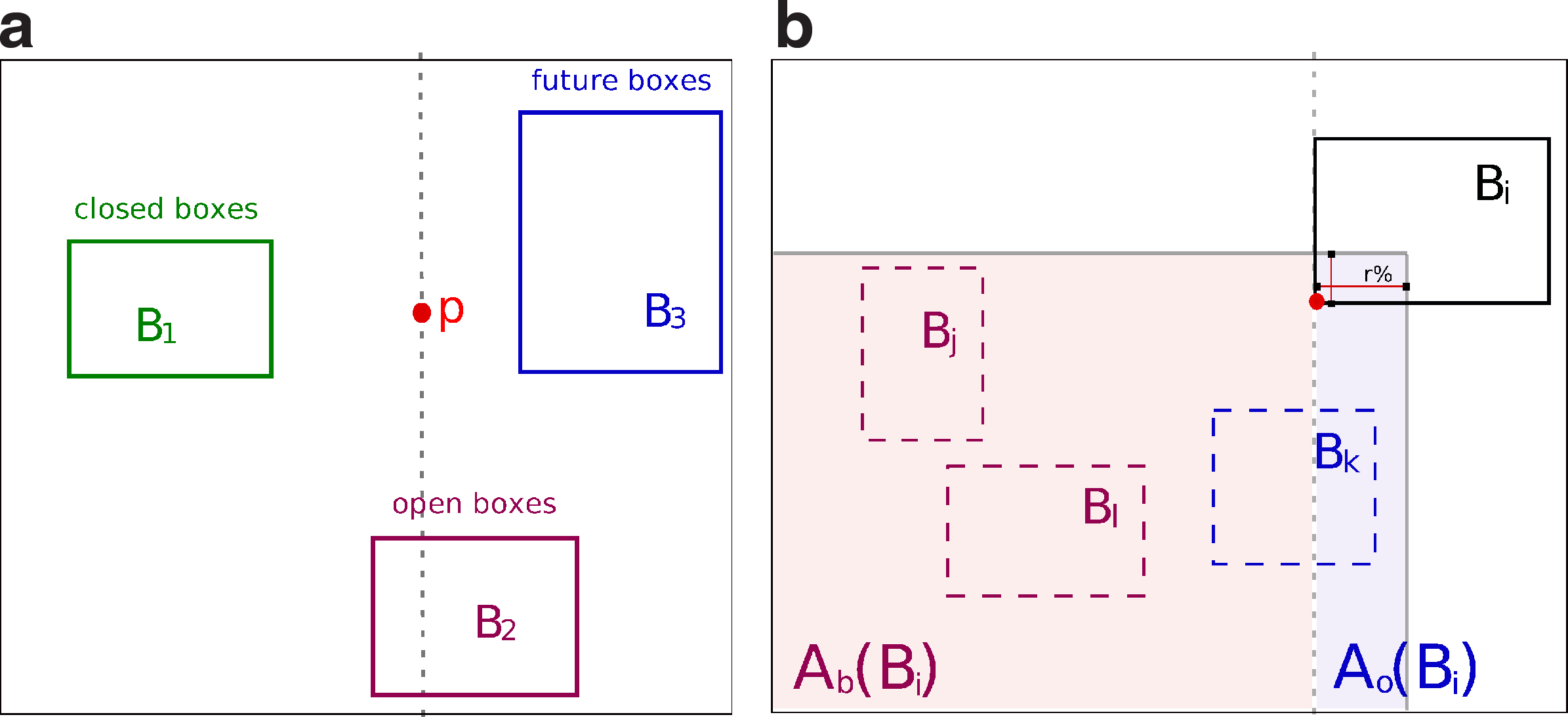
Let \documentclass{aastex}\usepackage{amsbsy}\usepackage{amsfonts}\usepackage{amssymb}\usepackage{bm}\usepackage{mathrsfs}\usepackage{pifont}\usepackage{stmaryrd}\usepackage{textcomp}\usepackage{portland, xspace}\usepackage{amsmath, amsxtra}\pagestyle{empty}\DeclareMathSizes{10}{9}{7}{6}\begin{document}$${ \cal P}$$\end{document} be an array containing the 2n points corresponding to l() and u() corners of the n boxes in \documentclass{aastex}\usepackage{amsbsy}\usepackage{amsfonts}\usepackage{amssymb}\usepackage{bm}\usepackage{mathrsfs}\usepackage{pifont}\usepackage{stmaryrd}\usepackage{textcomp}\usepackage{portland, xspace}\usepackage{amsmath, amsxtra}\pagestyle{empty}\DeclareMathSizes{10}{9}{7}{6}\begin{document}$${ \cal B}$$\end{document}. Points in \documentclass{aastex}\usepackage{amsbsy}\usepackage{amsfonts}\usepackage{amssymb}\usepackage{bm}\usepackage{mathrsfs}\usepackage{pifont}\usepackage{stmaryrd}\usepackage{textcomp}\usepackage{portland, xspace}\usepackage{amsmath, amsxtra}\pagestyle{empty}\DeclareMathSizes{10}{9}{7}{6}\begin{document}$${ \cal P}$$\end{document} are ordered on their x-coordinates; among the points having identical x-coordinates, lower corners are placed before upper corners. For each point, we store to which box and to which corner it corresponds to. In Algorithm 1, the main loop sweeps the points of \documentclass{aastex}\usepackage{amsbsy}\usepackage{amsfonts}\usepackage{amssymb}\usepackage{bm}\usepackage{mathrsfs}\usepackage{pifont}\usepackage{stmaryrd}\usepackage{textcomp}\usepackage{portland, xspace}\usepackage{amsmath, amsxtra}\pagestyle{empty}\DeclareMathSizes{10}{9}{7}{6}\begin{document}$${ \cal P}$$\end{document} and processes in a different manner lower (lines 5–8) and upper corners (lines 9–21). We say a box Bx is open when the sweep line is located between l(Bx) and u(Bx) inclusive, closed when the line has passed u(Bx), and future when it lies before l(Bx). These states are exclusive of each other, and partition at each moment \documentclass{aastex}\usepackage{amsbsy}\usepackage{amsfonts}\usepackage{amssymb}\usepackage{bm}\usepackage{mathrsfs}\usepackage{pifont}\usepackage{stmaryrd}\usepackage{textcomp}\usepackage{portland, xspace}\usepackage{amsmath, amsxtra}\pagestyle{empty}\DeclareMathSizes{10}{9}{7}{6}\begin{document}$${ \cal B}$$\end{document} in three disjoint sets (Fig. 1a). All open boxes at each point are kept in a set \documentclass{aastex}\usepackage{amsbsy}\usepackage{amsfonts}\usepackage{amssymb}\usepackage{bm}\usepackage{mathrsfs}\usepackage{pifont}\usepackage{stmaryrd}\usepackage{textcomp}\usepackage{portland, xspace}\usepackage{amsmath, amsxtra}\pagestyle{empty}\DeclareMathSizes{10}{9}{7}{6}\begin{document}$${ \cal O}$$\end{document} (lines 6, 10). The weight of a chain ending at, say Bi, and passing by a predecessor of Bi, Bx, can only be computed when Bx is closed (when W[Bx] has reached its final value). If P1(u(Bx)) < P1(l(Bi)) then this can be done when stopping at l(Bi) (lines 7–8), while if Bx overlaps Bi on x-axis, then this is done when stopping at u(Bx), and at the same time for all open boxes having Bx as predecessor (lines 11–15). These two cases partition the possible predecessors of Bi according to the location of their upper corners in two areas Ab(Bi) and Ao(Bi) (Fig. 1b).
(a) Example of boxes in each disjoint set forming a partition of \documentclass{aastex}\usepackage{amsbsy}\usepackage{amsfonts}\usepackage{amssymb}\usepackage{bm}\usepackage{mathrsfs}\usepackage{pifont}\usepackage{stmaryrd}\usepackage{textcomp}\usepackage{portland, xspace}\usepackage{amsmath, amsxtra}\pagestyle{empty}\DeclareMathSizes{10}{9}{7}{6}\begin{document}$${ \cal B}$$\end{document}, when sweeping a point p. (b) Partition of the search space of possible predecessors of Bi in two areas, Ab(Bi) and Ao(Bi), according to the location of their upper corners: Ab(Bi) at left from the dashed line, and Ao(Bi) at its right.
As above mentioned, we maintain in \documentclass{aastex}\usepackage{amsbsy}\usepackage{amsfonts}\usepackage{amssymb}\usepackage{bm}\usepackage{mathrsfs}\usepackage{pifont}\usepackage{stmaryrd}\usepackage{textcomp}\usepackage{portland, xspace}\usepackage{amsmath, amsxtra}\pagestyle{empty}\DeclareMathSizes{10}{9}{7}{6}\begin{document}$${ \cal A}$$\end{document} the set of interesting predecessors for all future boxes. Boxes in \documentclass{aastex}\usepackage{amsbsy}\usepackage{amsfonts}\usepackage{amssymb}\usepackage{bm}\usepackage{mathrsfs}\usepackage{pifont}\usepackage{stmaryrd}\usepackage{textcomp}\usepackage{portland, xspace}\usepackage{amsmath, amsxtra}\pagestyle{empty}\DeclareMathSizes{10}{9}{7}{6}\begin{document}$${ \cal A}$$\end{document} are active boxes. Hence, once closing a box (stopping at its upper corner), we test whether it should be turned active and inserted in \documentclass{aastex}\usepackage{amsbsy}\usepackage{amsfonts}\usepackage{amssymb}\usepackage{bm}\usepackage{mathrsfs}\usepackage{pifont}\usepackage{stmaryrd}\usepackage{textcomp}\usepackage{portland, xspace}\usepackage{amsmath, amsxtra}\pagestyle{empty}\DeclareMathSizes{10}{9}{7}{6}\begin{document}$${ \mathcal A}$$\end{document} (lines 16–18). The current box, Bi, is inserted only if we cannot find a better predecessor in \documentclass{aastex}\usepackage{amsbsy}\usepackage{amsfonts}\usepackage{amssymb}\usepackage{bm}\usepackage{mathrsfs}\usepackage{pifont}\usepackage{stmaryrd}\usepackage{textcomp}\usepackage{portland, xspace}\usepackage{amsmath, amsxtra}\pagestyle{empty}\DeclareMathSizes{10}{9}{7}{6}\begin{document}$${ \cal A}$$\end{document}. Afterwards, if Bi has been added, currently active boxes are investigated to determine if they are less interesting than Bi, in which case they are deleted from \documentclass{aastex}\usepackage{amsbsy}\usepackage{amsfonts}\usepackage{amssymb}\usepackage{bm}\usepackage{mathrsfs}\usepackage{pifont}\usepackage{stmaryrd}\usepackage{textcomp}\usepackage{portland, xspace}\usepackage{amsmath, amsxtra}\pagestyle{empty}\DeclareMathSizes{10}{9}{7}{6}\begin{document}$${ \cal A}$$\end{document} (lines 19–21). Active boxes are consulted when opening a box Bi, for computing the best chain ending at Bi with a predecessor in Ab(Bi) (lines 7–8).
4.2. Correctness of the algorithm
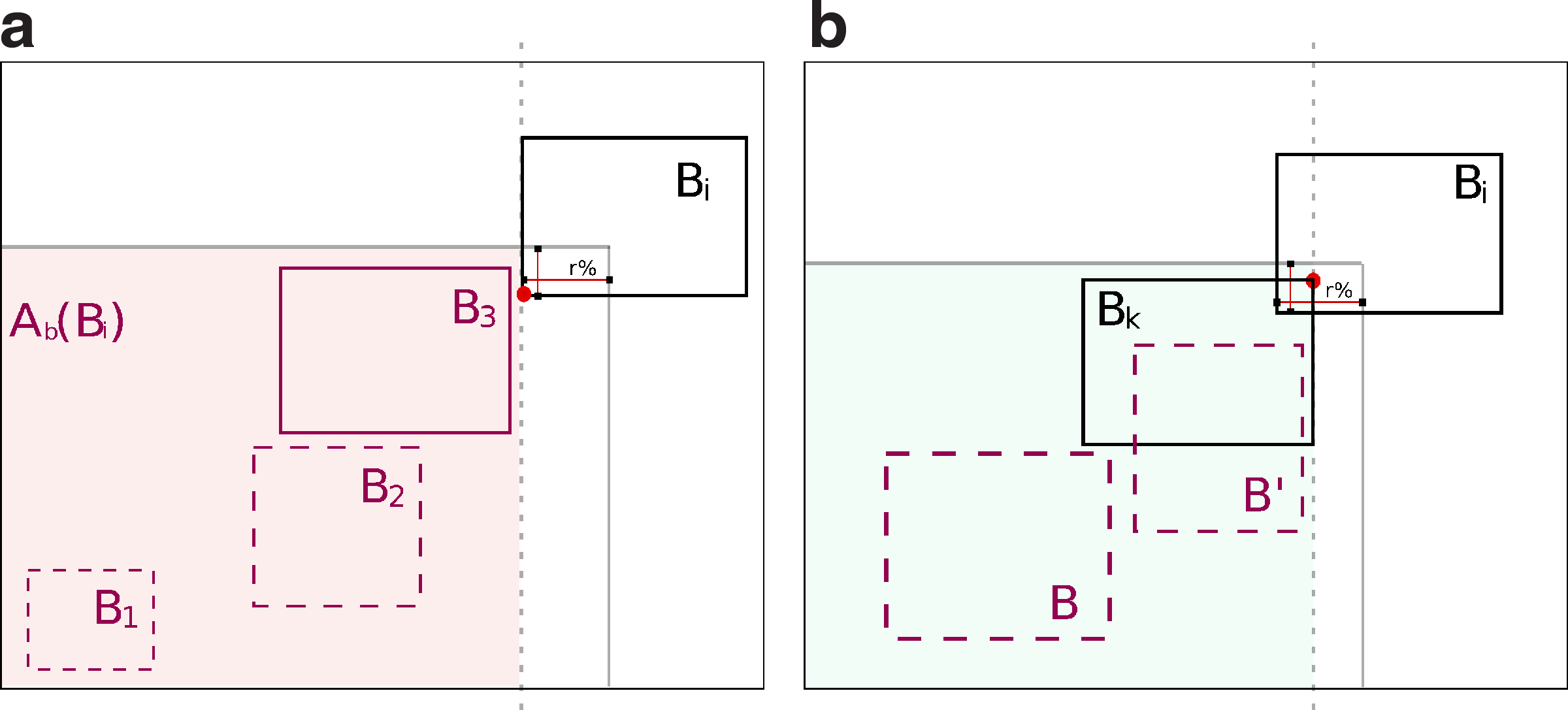
For 1 ≤ i ≤ n, we show that W[Bi] and Pred[Bi] store the weight and the predecessor of Bi in a maximum weighted chain ending at Bi. First, several simple invariants emerge from Algorithm 1. I1: At any point, the set \documentclass{aastex}\usepackage{amsbsy}\usepackage{amsfonts}\usepackage{amssymb}\usepackage{bm}\usepackage{mathrsfs}\usepackage{pifont}\usepackage{stmaryrd}\usepackage{textcomp}\usepackage{portland, xspace}\usepackage{amsmath, amsxtra}\pagestyle{empty}\DeclareMathSizes{10}{9}{7}{6}\begin{document}$${ \cal O}$$\end{document} contains all open boxes. I2: Both W[Bi] and Pred[Bi] store their final values once u(Bi) has been processed, since they are not altered after that point. I3: Hence, at any point all active boxes (i.e., boxes in \documentclass{aastex}\usepackage{amsbsy}\usepackage{amsfonts}\usepackage{amssymb}\usepackage{bm}\usepackage{mathrsfs}\usepackage{pifont}\usepackage{stmaryrd}\usepackage{textcomp}\usepackage{portland, xspace}\usepackage{amsmath, amsxtra}\pagestyle{empty}\DeclareMathSizes{10}{9}{7}{6}\begin{document}$${ \cal A}$$\end{document}), which are closed boxes, satisfy I2. For conciseness, as W[Bi] and Pred[Bi] are computed jointly, from now on we deal only with W[Bi]. Since potential predecessors of Bi are partitioned in Ab(Bi) (Fig. 2a) and Ao(Bi) (Fig. 2b), we will prove two invariants: I4: partial optimality over Ab(Bi) at lower corners, and I5: optimality at upper corners.
(a) When passing l(Bi), Pred[Bi] is a partial optimum on the set of possible predecessors of Bi lying in Ab(Bi) (in the example, B3). (b) When passing u(Bk), Pred[Bi] is a partial optimum on the set of possible predecessors of Bi from \documentclass{aastex}\usepackage{amsbsy}\usepackage{amsfonts}\usepackage{amssymb}\usepackage{bm}\usepackage{mathrsfs}\usepackage{pifont}\usepackage{stmaryrd}\usepackage{textcomp}\usepackage{portland, xspace}\usepackage{amsmath, amsxtra}\pagestyle{empty}\DeclareMathSizes{10}{9}{7}{6}\begin{document}$$A_b ( B_i ) \cup \{ B \in A_o ( B_i ) / P_1 ( u ( B ) ) < P_1 ( u ( B_k ) ) \} $$\end{document}.
I4: partial optimality over Ab(Bi) at lower corners
We show that after processing l(Bi), W[Bi] stores the weight of a maximum weighted chain ending at Bi with predecessor in Ab(Bi). Given line 7, this is equivalent to showing that no better chain ending at Bi passes through a potential predecessor that does not belong to \documentclass{aastex}\usepackage{amsbsy}\usepackage{amsfonts}\usepackage{amssymb}\usepackage{bm}\usepackage{mathrsfs}\usepackage{pifont}\usepackage{stmaryrd}\usepackage{textcomp}\usepackage{portland, xspace}\usepackage{amsmath, amsxtra}\pagestyle{empty}\DeclareMathSizes{10}{9}{7}{6}\begin{document}$${ \cal A}$$\end{document} at that point, which we prove by contradiction. While processing l(Bi), \documentclass{aastex}\usepackage{amsbsy}\usepackage{amsfonts}\usepackage{amssymb}\usepackage{bm}\usepackage{mathrsfs}\usepackage{pifont}\usepackage{stmaryrd}\usepackage{textcomp}\usepackage{portland, xspace}\usepackage{amsmath, amsxtra}\pagestyle{empty}\DeclareMathSizes{10}{9}{7}{6}\begin{document}$${ \cal A}$$\end{document} contains a subset of boxes in Ab(Bi), but obviously none from Ao(Bi). Let B be a closed box of \documentclass{aastex}\usepackage{amsbsy}\usepackage{amsfonts}\usepackage{amssymb}\usepackage{bm}\usepackage{mathrsfs}\usepackage{pifont}\usepackage{stmaryrd}\usepackage{textcomp}\usepackage{portland, xspace}\usepackage{amsmath, amsxtra}\pagestyle{empty}\DeclareMathSizes{10}{9}{7}{6}\begin{document}$${ \cal B} \setminus { \cal A}$$\end{document} such that B≪rBi and w(Bi) − w(B ∩ Bi) + W[B] > W[Bi], in other words, B makes a better predecessor for Bi than those in \documentclass{aastex}\usepackage{amsbsy}\usepackage{amsfonts}\usepackage{amssymb}\usepackage{bm}\usepackage{mathrsfs}\usepackage{pifont}\usepackage{stmaryrd}\usepackage{textcomp}\usepackage{portland, xspace}\usepackage{amsmath, amsxtra}\pagestyle{empty}\DeclareMathSizes{10}{9}{7}{6}\begin{document}$${ \cal A}$$\end{document}. From B≪rBi, we get
\documentclass{aastex}\usepackage{amsbsy}\usepackage{amsfonts}\usepackage{amssymb}\usepackage{bm}\usepackage{mathrsfs}\usepackage{pifont}\usepackage{stmaryrd}\usepackage{textcomp}\usepackage{portland,xspace}\usepackage{amsmath,amsxtra}\pagestyle{empty}\DeclareMathSizes{10}{9}{7}{6}\begin{document}\begin{align*}
P_2 ( u ( B ) ) - P_2 ( l ( B_i ) ) \leq r \min ( \mid P_2 ( B )
\mid , \mid P_2 ( B_i ) \mid ) . \tag{5}
\end{align*}\end{document}
As only two possibilities exist for B not belonging to \documentclass{aastex}\usepackage{amsbsy}\usepackage{amsfonts}\usepackage{amssymb}\usepackage{bm}\usepackage{mathrsfs}\usepackage{pifont}\usepackage{stmaryrd}\usepackage{textcomp}\usepackage{portland, xspace}\usepackage{amsmath, amsxtra}\pagestyle{empty}\DeclareMathSizes{10}{9}{7}{6}\begin{document}$${ \cal A}$$\end{document}, we distinguish two exclusive cases.
B was not turned active when sweeping u(B) (lines 16–18)
B did not satisfy the condition on line 17. Let \documentclass{aastex}\usepackage{amsbsy}\usepackage{amsfonts}\usepackage{amssymb}\usepackage{bm}\usepackage{mathrsfs}\usepackage{pifont}\usepackage{stmaryrd}\usepackage{textcomp}\usepackage{portland, xspace}\usepackage{amsmath, amsxtra}\pagestyle{empty}\DeclareMathSizes{10}{9}{7}{6}\begin{document}$$B^{ \prime} : = \mathop{ \rm arg\ max} \limits_{B_j \in { \cal A}: u ( B_j ) < u ( B ) } ( W [ B_j ] )$$\end{document}. Our hypothesis means that u(B′) < u(B) and
\documentclass{aastex}\usepackage{amsbsy}\usepackage{amsfonts}\usepackage{amssymb}\usepackage{bm}\usepackage{mathrsfs}\usepackage{pifont}\usepackage{stmaryrd}\usepackage{textcomp}\usepackage{portland,xspace}\usepackage{amsmath,amsxtra}\pagestyle{empty}\DeclareMathSizes{10}{9}{7}{6}\begin{document}\begin{align*}
W [ B ] < W [ B^{ \prime} ] \tag{6}
\end{align*}\end{document}\documentclass{aastex}\usepackage{amsbsy}\usepackage{amsfonts}\usepackage{amssymb}\usepackage{bm}\usepackage{mathrsfs}\usepackage{pifont}\usepackage{stmaryrd}\usepackage{textcomp}\usepackage{portland,xspace}\usepackage{amsmath,amsxtra}\pagestyle{empty}\DeclareMathSizes{10}{9}{7}{6}\begin{document}\begin{align*}
\mid P_2 ( B ) \mid \leq \mid P_2 ( B^{ \prime} ) \mid . \tag{7}
\end{align*}\end{document}
For B does not overlap Bi and u(B′) < u(B), we have B′ does not overlap Bi on the x-axis. From u(B′) < u(B), we get P2(u(B′)) < P2(u(B)); this with equations 5 and 7 yields
\documentclass{aastex}\usepackage{amsbsy}\usepackage{amsfonts}\usepackage{amssymb}\usepackage{bm}\usepackage{mathrsfs}\usepackage{pifont}\usepackage{stmaryrd}\usepackage{textcomp}\usepackage{portland,xspace}\usepackage{amsmath,amsxtra}\pagestyle{empty}\DeclareMathSizes{10}{9}{7}{6}\begin{document}\begin{align*}
P_2 ( u ( B^{ \prime} ) ) - P_2 ( l ( B_i ) ) & < P_2 ( u ( B ) )
- P_2 ( l ( B_i ) ) \\ & \leq r \min ( \mid P_2 ( B ) \mid , \mid
P_2 ( B_i ) \mid ) \\ & \leq r \min ( \mid P_2 ( B^{ \prime} )
\mid , \mid P_2 ( B_i ) \mid ) . \tag{8}
\end{align*}\end{document}
Equation 8 and B′ not overlapping Bi on the x-axis imply B′≪rBi. Finally, from equations 6, 7, and u(B′) < u(B), we obtain:
\documentclass{aastex}\usepackage{amsbsy}\usepackage{amsfonts}\usepackage{amssymb}\usepackage{bm}\usepackage{mathrsfs}\usepackage{pifont}\usepackage{stmaryrd}\usepackage{textcomp}\usepackage{portland,xspace}\usepackage{amsmath,amsxtra}\pagestyle{empty}\DeclareMathSizes{10}{9}{7}{6}\begin{document}\begin{align*}
W [ B ] + \sum \limits_{ \alpha = 1}^2 ( w_{ \alpha} ( B_i ) - w_{
\alpha} ( B_i \cap B ) ) < W [ B^{ \prime} ] + \sum \limits_{
\alpha = 1}^2 ( w_{ \alpha} ( B_i ) - w_{ \alpha} ( B_i \cap
B^{\prime} ) ) ,
\end{align*}\end{document}
and thus B′ makes a better predecessor for Bi than B, a contradiction.
B was inactivated when sweeping u(Bk) for some box Bk ending before l(Bi) (lines 19–21)
The hypothesis means that B was deleted from \documentclass{aastex}\usepackage{amsbsy}\usepackage{amsfonts}\usepackage{amssymb}\usepackage{bm}\usepackage{mathrsfs}\usepackage{pifont}\usepackage{stmaryrd}\usepackage{textcomp}\usepackage{portland, xspace}\usepackage{amsmath, amsxtra}\pagestyle{empty}\DeclareMathSizes{10}{9}{7}{6}\begin{document}$${ \cal A}$$\end{document} for it satisfied P2(u(Bk)) < P2(u(B)), W[B] < W[Bk], and at least one of the conditions (a) |P2(B)| < |P2(Bk)| or (b) P2(u(Bk)) < P2(l(B)).
(a) As above (see Eq. 8), from Equation 6, from |P2(B)| < |P2(Bk)|, and P2(u(Bk)) < P2(u(B)), we get
\documentclass{aastex}\usepackage{amsbsy}\usepackage{amsfonts}\usepackage{amssymb}\usepackage{bm}\usepackage{mathrsfs}\usepackage{pifont}\usepackage{stmaryrd}\usepackage{textcomp}\usepackage{portland,xspace}\usepackage{amsmath,amsxtra}\pagestyle{empty}\DeclareMathSizes{10}{9}{7}{6}\begin{document}\begin{align*}
P_2 ( u ( B_k ) ) - P_2 ( l ( B_i ) ) < r \min ( \mid P_2 ( B_k )
\mid , \mid P_2 ( B_i ) \mid ) . \tag{9}
\end{align*}\end{document}
Moreover, as Bk does not overlap Bi on the x-axis, we obtain Bk≪rBi. As P2(u(Bk)) < P2(u(B)), Bk and B do not overlap Bi on x-axis, and W[B] < W[Bk], we finally derive
\documentclass{aastex}\usepackage{amsbsy}\usepackage{amsfonts}\usepackage{amssymb}\usepackage{bm}\usepackage{mathrsfs}\usepackage{pifont}\usepackage{stmaryrd}\usepackage{textcomp}\usepackage{portland,xspace}\usepackage{amsmath,amsxtra}\pagestyle{empty}\DeclareMathSizes{10}{9}{7}{6}\begin{document}\begin{align*}
W [ B ] + \sum \limits_{ \alpha = 1}^2 \mid P_{ \alpha} ( B_i )
\setminus P_{ \alpha} ( B ) \mid ) < W [ B_k ] + \sum \limits_{
\alpha = 1}^2 \mid P_{ \alpha} ( B_i ) \setminus P_{ \alpha} ( B_k
) \mid ) . \tag{10}
\end{align*}\end{document}
(b) By hypothesis, we know that P2(u(Bk)) < P2(l(B)) < P2(l(Bi)), and since neither Bk nor B overlap Bi on the x-axis, we directly obtain Bk ≪ Bi (Bi ∩ Bk = ∅). Thus, W[B] < W[Bk] also implies Equation 10.
With either condition (a) or (b), Bk makes a better predecessor for Bi than B, a contradiction.
Finally, after processing l(Bi), W[Bi] stores the weight of a maximum weighted chain ending at Bi with predecessor in Ab(Bi), which concludes the proof of I4.
I5: optimality at upper corners
We show that after processing u(Bi), W[Bi] stores W(Bi) (a Maximum Weighted Chain with a predecessor in Ab(Bi) ∪ Ao(Bi)). As all predecessors of Bi are closed, let us denote by B, the right most predecessor of Bi on the x-axis: \documentclass{aastex}\usepackage{amsbsy}\usepackage{amsfonts}\usepackage{amssymb}\usepackage{bm}\usepackage{mathrsfs}\usepackage{pifont}\usepackage{stmaryrd}\usepackage{textcomp}\usepackage{portland, xspace}\usepackage{amsmath, amsxtra}\pagestyle{empty}\DeclareMathSizes{10}{9}{7}{6}\begin{document}$$B : = {\rm arg\ max}_{B_j \ll_r B_i} ( P_1 ( u ( B_j ) ) )$$\end{document}.
1. If \documentclass{aastex}\usepackage{amsbsy}\usepackage{amsfonts}\usepackage{amssymb}\usepackage{bm}\usepackage{mathrsfs}\usepackage{pifont}\usepackage{stmaryrd}\usepackage{textcomp}\usepackage{portland, xspace}\usepackage{amsmath, amsxtra}\pagestyle{empty}\DeclareMathSizes{10}{9}{7}{6}\begin{document}$$u ( B ) \in A_b ( B_i )$$\end{document} then all predecessors of Bi are contained in Ab(Bi). Hence, this situation was handled when processing l(Bi), and Invariant I4 regarding the partial optimality at lower corners, ensures that W[Bi] stores W(Bi).
2. If \documentclass{aastex}\usepackage{amsbsy}\usepackage{amsfonts}\usepackage{amssymb}\usepackage{bm}\usepackage{mathrsfs}\usepackage{pifont}\usepackage{stmaryrd}\usepackage{textcomp}\usepackage{portland, xspace}\usepackage{amsmath, amsxtra}\pagestyle{empty}\DeclareMathSizes{10}{9}{7}{6}\begin{document}$$u ( B ) \in A_o ( B_i )$$\end{document}, W[Bi] has been correctly updated (lines 11–15), while Bi was open, when sweeping u(Bk) for each box \documentclass{aastex}\usepackage{amsbsy}\usepackage{amsfonts}\usepackage{amssymb}\usepackage{bm}\usepackage{mathrsfs}\usepackage{pifont}\usepackage{stmaryrd}\usepackage{textcomp}\usepackage{portland, xspace}\usepackage{amsmath, amsxtra}\pagestyle{empty}\DeclareMathSizes{10}{9}{7}{6}\begin{document}$$B_k \in { \cal B}$$\end{document} such that Bk≪rBi and \documentclass{aastex}\usepackage{amsbsy}\usepackage{amsfonts}\usepackage{amssymb}\usepackage{bm}\usepackage{mathrsfs}\usepackage{pifont}\usepackage{stmaryrd}\usepackage{textcomp}\usepackage{portland, xspace}\usepackage{amsmath, amsxtra}\pagestyle{empty}\DeclareMathSizes{10}{9}{7}{6}\begin{document}$$u ( B_k ) \in A_o ( B_i )$$\end{document}.
Hence, all predecessors of Bi have been taken into account, and W[Bi] stores W(Bi). This concludes the proof of I5, and closes the correctness proof.
4.3. Time and space analysis
Here, we detail the complexities of our sweep-line algorithm (Algorithm 1) and compare it to the dynamic programming algorithm (Algorithm DP) in term of running time.
Obviously, the sets \documentclass{aastex}\usepackage{amsbsy}\usepackage{amsfonts}\usepackage{amssymb}\usepackage{bm}\usepackage{mathrsfs}\usepackage{pifont}\usepackage{stmaryrd}\usepackage{textcomp}\usepackage{portland, xspace}\usepackage{amsmath, amsxtra}\pagestyle{empty}\DeclareMathSizes{10}{9}{7}{6}\begin{document}$${ \cal O}$$\end{document} and \documentclass{aastex}\usepackage{amsbsy}\usepackage{amsfonts}\usepackage{amssymb}\usepackage{bm}\usepackage{mathrsfs}\usepackage{pifont}\usepackage{stmaryrd}\usepackage{textcomp}\usepackage{portland, xspace}\usepackage{amsmath, amsxtra}\pagestyle{empty}\DeclareMathSizes{10}{9}{7}{6}\begin{document}$${ \cal A}$$\end{document} contain at most n boxes, and thus require together with arrays Pred[.] and W[.], O(n) space. We use balanced binary search trees (BST) to store \documentclass{aastex}\usepackage{amsbsy}\usepackage{amsfonts}\usepackage{amssymb}\usepackage{bm}\usepackage{mathrsfs}\usepackage{pifont}\usepackage{stmaryrd}\usepackage{textcomp}\usepackage{portland, xspace}\usepackage{amsmath, amsxtra}\pagestyle{empty}\DeclareMathSizes{10}{9}{7}{6}\begin{document}$${ \cal A}$$\end{document} and \documentclass{aastex}\usepackage{amsbsy}\usepackage{amsfonts}\usepackage{amssymb}\usepackage{bm}\usepackage{mathrsfs}\usepackage{pifont}\usepackage{stmaryrd}\usepackage{textcomp}\usepackage{portland, xspace}\usepackage{amsmath, amsxtra}\pagestyle{empty}\DeclareMathSizes{10}{9}{7}{6}\begin{document}$${ \cal O}$$\end{document}, with boxes at the leaves ordered on P2(u(.)), respectively P1(l(.)). Hence, the amortized time needed for all insertions, deletions, and rebalancing is O(n log n) (Knuth, 1998). However, looking for the active boxes that can be deleted at each execution of the outer loop (lines 19–21) may force us to examine all boxes in \documentclass{aastex}\usepackage{amsbsy}\usepackage{amsfonts}\usepackage{amssymb}\usepackage{bm}\usepackage{mathrsfs}\usepackage{pifont}\usepackage{stmaryrd}\usepackage{textcomp}\usepackage{portland, xspace}\usepackage{amsmath, amsxtra}\pagestyle{empty}\DeclareMathSizes{10}{9}{7}{6}\begin{document}$${ \cal A}$$\end{document}. As this is the more complex operation in the outer loop, we obtain in the worst case an O(n2) time and O(n) space complexity. Algorithm 1 maintains the subset of potential predecessors in \documentclass{aastex}\usepackage{amsbsy}\usepackage{amsfonts}\usepackage{amssymb}\usepackage{bm}\usepackage{mathrsfs}\usepackage{pifont}\usepackage{stmaryrd}\usepackage{textcomp}\usepackage{portland, xspace}\usepackage{amsmath, amsxtra}\pagestyle{empty}\DeclareMathSizes{10}{9}{7}{6}\begin{document}$${ \cal A}$$\end{document} instead of searching through the whole box set as in Algorithm DP, which makes the practical difference.
The experimental running times observed when performing 694 whole genome pairwise comparisons (see Section 5) show that this optimisation yields significant improvements: Algorithm 1 needed ≈8 hours to compute the 694 chains, while Algorithm DP took 3.5 days for the same computation. The improvement increases with the number of input fragments, and becomes considerable above 50, 000 fragments. In fact, below 50, 000 fragments, both Algorithm 1 and Algorithm DP take seconds, i.e., less than 1 minute. However, for n ranging from 50, 000 to 100, 000 Algorithm 1 still takes less than a minute, while Algorithm DP needs 1–6 minutes to compute the chain.
Moreover, the gap between the two algorithms is widening beyond the threshold of 100, 000 fragments. The following examples illustrate this statement: for a pair of strains (CP000011 vs. CP000548) from Burkholderia mallei species for which we computed 144, 685 fragments, Algorithm DP takes ≈16 minutes, while Algorithm 1 only needs less than 1 minute; for two strains from Burkholderia pseudomallei species (CP000573 vs. CP000125) with n = 197, 310 fragments, Algorithm DP takes 34 minutes and Algorithm 1 less than 3 minutes; for Neisseria meningitidis species (AM421808 vs. AE002098) having n = 307, 852, Algorithm DP needs 57 minutes and Algorithm 1 only 7 minutes. Finally, for a couple of strains (BX248333 vs. AM408590) from Mycobacterium bovis with 1, 000, 000 fragments, Algorithm 1 needs ≈1 hour, while Algorithm DP ended after 12 hours. More details on the running times of Algorithm 1 can be found in Figure 3b.
(a) Differences in coverage obtained on 694 bacterial genome comparisons between our algorithm and the classical chaining, presented as a box-and-whiskers plot: in 50% of the cases, allowing for proportional overlaps increases the coverage% with more than 15%. (b) Running times in seconds of our algorithm: in 75% of the cases, the algorithm needs less than 10 seconds.
5. Results
The comparison set we use for the the experiments below (and for those in the previous section) consists of all pairwise genome comparisons of strains of the same bacteria (intra-species comparisons) as of January 2010, i.e., 694 pairwise genome comparisons. It comprises 346 different genomes from 88 species retrieved from Genome Reviews database (Kersey et al., 2005). We first computed the local alignments in every genome pair, by using YASS with default parameters (Noé and Kucherov, 2005). The output local alignments are the fragments given as input to the chaining step.
A first issue we examine in this section is in which measure allowing for overlaps improves the chain weight (here, the genome coverage) when comparing genomes, and at which computational cost. To investigate this, we compared the running times, the coverage% (for a definition of coverage, see second page of this article) and the identity% on 694 pairwise genome comparisons, obtained with Chainer (Abouelhoda and Ohlebusch, 2005) when overlaps are not allowed, and with Algorithm 1, implemented in our tool OC, when proportional overlaps are taken into account. Here, we define the identity% as the ratio between the number of pairs of identical positions in the covered regions and the genomes' lengths.
For this first experiment, we ran in parallel Chainer and Algorithm 1, with the weight of a fragment on each genome being the length of the aligned sequence. We authorized overlaps measuring up to 10% of the fragments' lengths (r = 0.1). Hence, the total chain weight, i.e., the sum of the chained fragments lengths minus the overlaps, computed by the chaining step gives the genome coverage, which we report as a percentage of the genome length. It is straightforward that, as both chaining algorithms provide an optimal solution in their setup, the coverage with overlaps is always larger than without overlaps. Similar to the coverage, the identity% is computed on the set of chained fragments.
In Figure 3a, we plot, for each genome pair, the difference of coverage percentages (the differences of identity% are not depicted in this paper) between both algorithms: Algorithm 1 coverage% − Chainer coverage%; for example, a value of 10 means that chaining with overlaps covers 10% more of the genome than chaining without overlaps. The box-and-whiskers plot shows that, for this collection of bacterial genome pairs, the improvement has a median of 15% and reaches values up to 60%. Since bacterial genomes have a median length of 2.8 Mbp, a difference of 1% means at least 28 Kbp of additionally aligned sequences. Thus, one can make the following basic estimation. Knowing that, on average, 87% of these genomes are coding and that bacterial genes are 1 Kbp long (Xu et al., 2006), 15% more coverage should involve 365 additional genes compared to a solution without overlaps; this is important from the biological perspective. Chainer takes less than 1 second in average and at most 17 seconds. We plot the running times of Algorithm 1 in Figure 3b: it stays below 10 seconds in 75% of the comparisons, and between 3 and 67 minutes in only 30 cases (those with a number of fragments ranging from >200,000 to 1,000,000). Thus, allowing for overlaps improves the coverage significantly at a reasonable cost.
A biological question regards the causes of overlaps. For example, when comparing two strains (CP000046 vs. BA000018) of Staphylococcus aureus, the classical chaining gives a coverage of 65%, where Algorithm 1 yields a 94% coverage. In fact, the chain obtained without allowing overlaps is interrupted by 17 holes of more than 10 Kbp each. For 14 of these holes, at least one large fragment (average size 37 Kbp) was not included in the chain, because of an overlap with an adjacent fragment on one or both genomes. All overlaps measure between 1 bp and 1.8 Kbp in length (average, 218 bp). This example shows that overlaps' lengths cannot be easily bounded by a constant, thus revealing the necessity of using proportional overlaps. If short overlaps are mostly due to random equality between base pairs on fragment ends, we observed that large overlaps are often caused by variable tandem repeat structures that differ in number of copies between the strains. Correctly aligning such structures without breaking the region in two overlapping fragments requires a more general alignment model and specific algorithms (Bérard and Rivals, 2003).
Another issue to investigate is the robustness of results with respect to the ratio of allowed overlaps. For this, we examine the results obtained with three different overlap ratios: 5% of the fragments' lengths (r = 0.05), 10% (r = 0.1), and 15% (r = 0.15) on the same set composed of 694 pairwise genome comparisons. Finally, we study the advantage due to the use of proportional overlaps compared to fixed overlaps. For this purpose, we modified our algorithm in order to allow a fixed maximal overlap between fragments, instead of a ratio of their lengths. This means that an overlap between two fragments is allowed if it is below the fixed maximal overlap size and does not entirely cover one of the fragments. We thus tested four maximal overlap thresholds: 10 bp, 100 bp, 1 Kbp, and 10 Kbp.
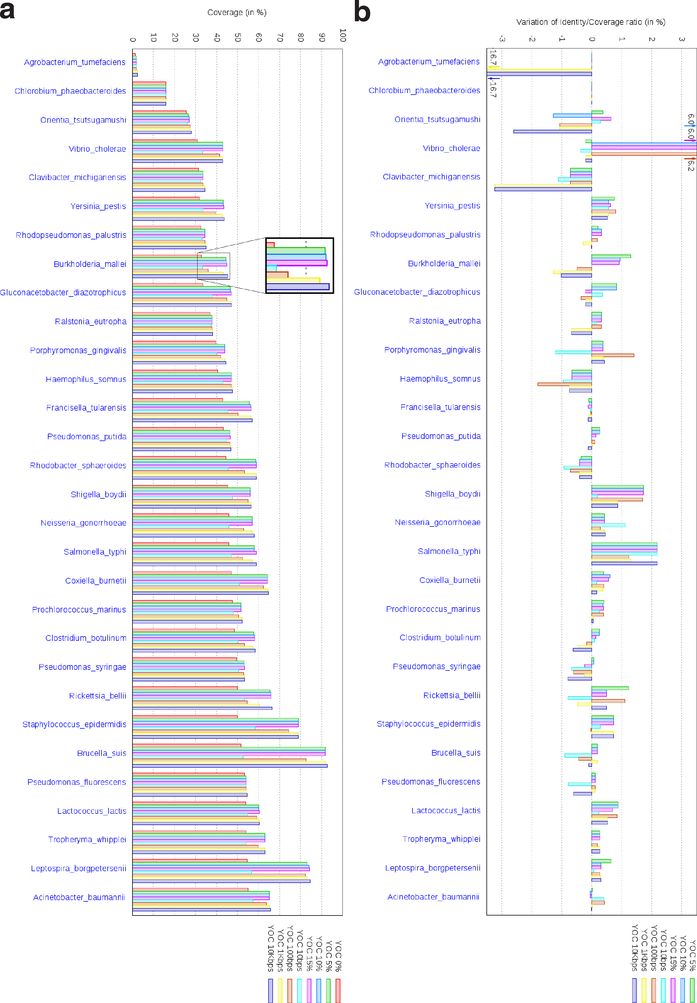
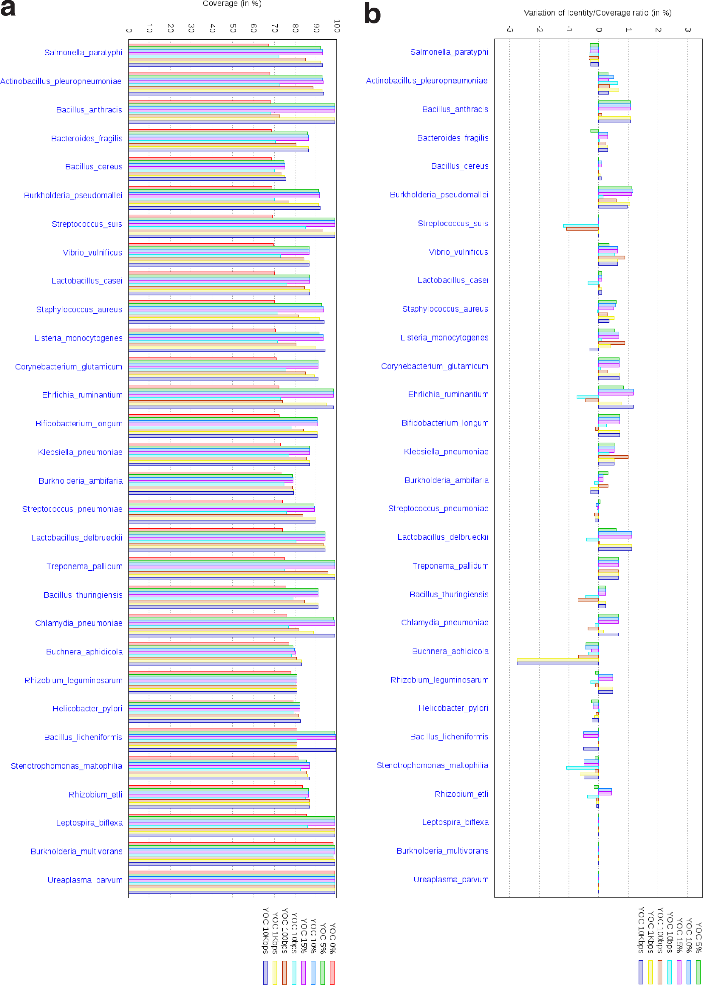
The results for different overlap ratios and fixed overlap thresholds are summarized in Figures 4–6, as averages on each one of the 88 species, for eight configurations of our program OC. These configurations correspond to a version without overlaps (OC 0%), a version with proportional overlaps for three overlap ratios (OC 5%, OC 10%, and OC 15%) and a version with fixed overlaps configured with four overlap thresholds (OC 10 bp, OC 100 bp, OC 1 Kbp, and OC 10 Kbp). In Figures 4–6, the results for the 88 species are partitioned for the sake of legibility as follows: 30 species in the first figure, 28 in the second one, and 30 in the third one. From the first figure to the third one, species are sorted on the average coverage% given by the version of the algorithm without overlaps (OC 0%). In the figures below, except studying the distribution of the coverage percentages, as chaining with overlaps covers additional genomic regions compared to overlap free chaining, it is important to assess the alignment quality of these regions. For this, we compute the ratio between the number of pairs of identical positions in the covered regions and their total length, which gives a quality measure of the covered regions. We use the following measure: assume an overlap chaining configuration yields a ratio of identical pairs over the length of the covered regions of X, while the overlap free chaining obtains a ratio of X0, then we compute the quality variation as (X − X0).
Average results for each species among 30 species, given by eight configurations of our program OC. (a) Variation of coverage %. Plots mainly show the robustness of results for different overlap ratios compared to fixed overlaps. (b) Variation of the ratios between the number of identities in the covered regions over the total length of these regions, relatively to OC 0%, showing that allowing overlaps does not imply covering lower quality regions.
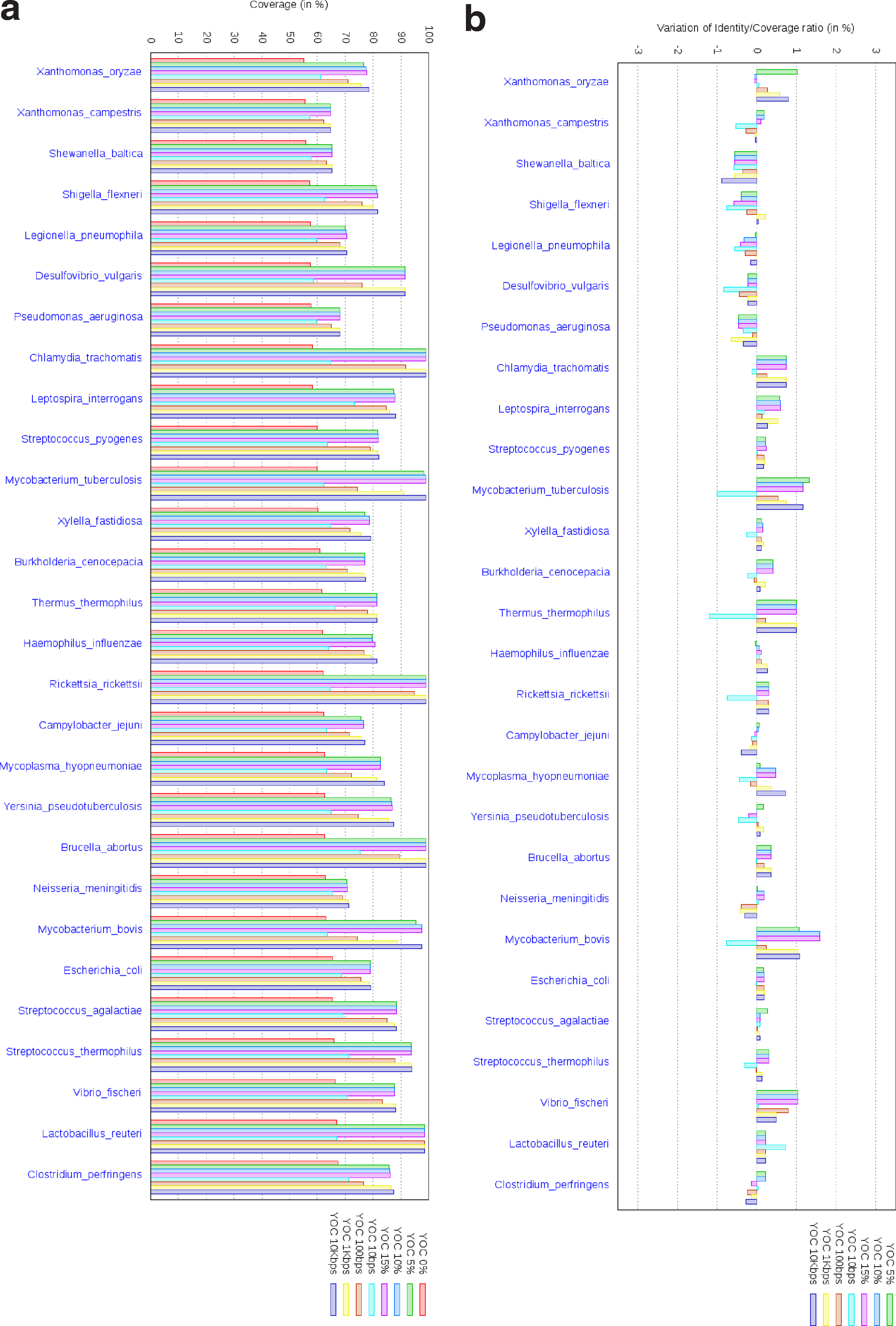
Similar to Figure 4, average results for each species among another 28 species, given by the eight configurations of our program, OC.
Similar to Figures 4 and 5, average results for each species among another 30 species, given by the eight configurations of our program, OC.
First, Figures 4a, 5a, and 6a show how the coverage percentages vary among the eight chaining configurations. Second, Figures 4b, 5b, and 6b report the quality variation of each overlap chaining configuration compared to overlap free chaining.
We chose to include the results for the whole dataset in order to illustrate the generality of our conclusions, at least for bacterial genomes. These figures must be considered as a whole, as it is important to understand that the following observations remain valid on all species:
• As already explained for Figure 3a, overlaps significantly improve the coverages, compared to overlap free chaining (mostly for proportional overlaps). This can be observed when examining the plots of the six configurations of OC compared to the version without overlaps, OC 0%. This trend is perfectly depicted in the zoom for Burkholderia mallei species in Figure 4a.
• Different overlap ratios generate very small variation among coverages: OC 5%, OC 10%, and OC 15% have very similar coverage values for all species. Thus, the total chain weight is robust to changes in the overlap ratio. Moreover, in most of the cases, these three configurations with proportional overlaps obtain coverages at least as high as the best of the other five configurations of OC. Clearly, the higher the maximal overlap ratio, the better the coverages are. However, if for small overlap ratios we observe a certain improvement, i.e., from 5 to 10, and below 5% (results not presented in this article), above 10%, improvements are not significant. Therefore, 10% seems to be a fair choice for the overlap ratio for bacterial comparisons, as overlaps in our dataset rarely reach 10% of fragments lengths.
• When dealing with fixed overlaps, one needs to set a relatively high threshold (10 Kbp) to get a slightly better coverage, especially when compared to the results obtained with proportional overlaps. OC 10 bp, OC 100 bp, and OC 1 Kbp systematically yield lower coverage than OC with proportional overlaps. Indeed, overlap sizes are widely distributed. Large overlaps are the ones penalizing the most the total coverage, as they prevent from incorporating large fragments into the chain. Hence, fixed overlap chaining can cope with such overlaps only if a high threshold is chosen, i.e., 10 Kbp. Moreover, the performance of fixed overlap solutions vary among genome pairs, making them less robust. Thus, fixed overlap thresholds are difficult to set. Comparatively, proportional overlap chaining proves more robust because of proportionality to fragments lengths.
• Importantly, the variation of quality compared to overlap free chaining (OC 0%) is quite small: between −2% and 2%, except for five cases that exhibit extremely low coverages (less than 5% coverage). Moreover, regarding quality variation, proportional overlaps configurations never yield the worst result among overlap chaining solutions. Thus, the alignment quality of covered regions remains stable when allowing proportional overlaps.
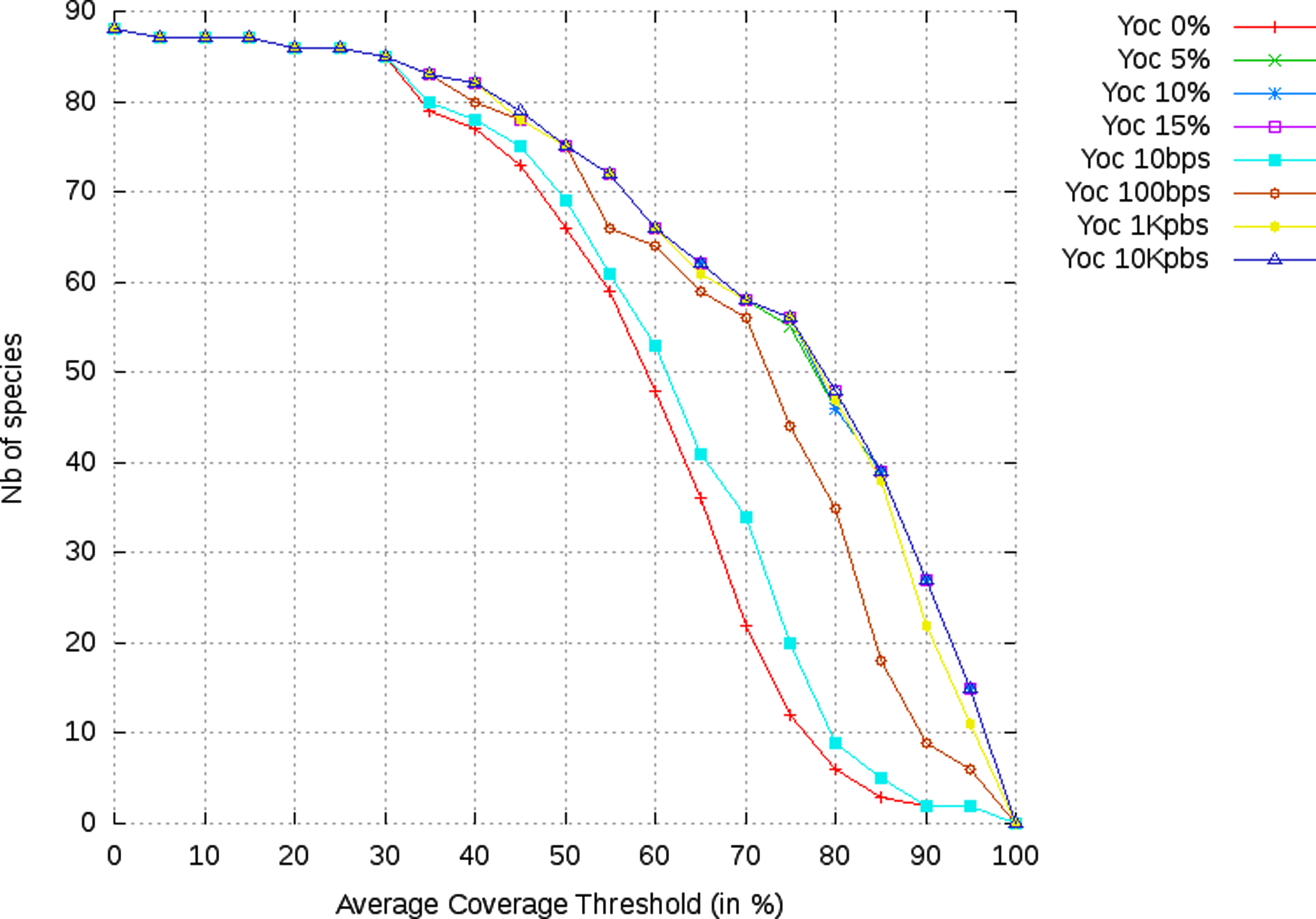
Finally, Figure 7 reports for each configuration of OC, the number of species whose computed chains reaches that coverage value, in average over all comparisons within that species. The red square at coordinates (60, 65) means that 65 species obtain a coverage of 60% with OC 100 bps threshold. All curves are superimposed in the range [0, 30] of coverage%. Beyond 30% coverage, the curves of proportional overlaps configurations are superimposed, again illustrating the robustness with respect to the overlap ratio. Moreover, above 30%, overlap free and fixed overlap chaining, except that with 10 Kbp threshold, generally perform worse than proportional overlap solutions.
The variation of the number of species for each coverage % threshold for the eight configurations of our program, OC.
6. Conclusion
To fulfill new needs in computational biology, we extended the classical framework of Maximum Weighted Chain by authorizing overlaps between fragments in the computed chain, and formalized the Maximum Weighted Chain with Proportional Length Overlaps problem where overlaps are proportional to the fragment lengths. Difficulties arise from the fact that the weights of overlaps are deduced from the chain weight. We exhibited the first two algorithms for this problem, which both solve it in quadratic time in function of the number of fragments. Experiments on a real dataset show that our sweep line algorithm outperforms the truly quadratic dynamic programming solution in practice. However, the study of the average time complexity of the sweep line algorithm remains open. By comparing the genome coverage obtained by different configurations of our program, OverlapChainer (OC), when applied to intra-species, bacterial comparisons, we observe that (i) overlaps improve significantly the coverage of genomes (median of 15%), while maintaining the same level of alignment quality; and (ii) results obtained with proportional overlaps are robust with respect to different overlap ratios, contrarily to fixed overlaps. This robustness may be explained by the limited overlap size in bacterial genomes comparisons. In the bacterial case, a ratio of 0.1 yield good results on a wide panel of 694 pairwise genome comparisons.
Investigating the performance of OverlapChainer on eukaryotic genomes is an interesting perspective and the same as studying the choice of the overlap ratio. Our algorithms can be extended for multiple genome comparisons; however, future research should also consider this case in practice. Moreover, the optimal complexity of chaining with proportional overlaps remains open.
Footnotes
Acknowledgments
This work was supported by the French National Research Agency (CoCoGen project; BLAN07-1_185484). A.M. and R.U. were also supported, respectively, by CNRS funding and a grant from the Ministry of Higher Education and Research of France.
Disclosure Statement
No competing financial interests exist.
References
1.
AbouelhodaM.I., OhlebuschE.2005. Chaining algorithms for multiple genome comparison. J. Discrete Algorithms, 3:321–341.
2.
BoussauB., DaubinV.2010. Genomes as documents of evolutionary history. Trends Ecol Evol., 25:224–232.
3.
BérardS., RivalsE.2003. Comparison of minisatellites. J. Comput. Biol., 10:357–372.
4.
CormenT.H., LeisersonC.E., RivestR.L.et al.2001. Introduction to Algorithms, 2nd. MIT Press: Cambridge, MA.
5.
FelsnerS., MullerR., WernischL.1995. Trapezoid graphs and generalizations, geometry and algorithms. Disc. Appl. Math., 74:13–32.
ShibuyaT., KurochkinI.2003. Match chaining algorithms for cDNA mapping. Lect. Notes Comput. Sci., 2812:462–475.
15.
UricaruR., MichoteyC., NoéL.et al.2009. Improved sensitivity and reliability of anchor based genome alignment. Actes J. Ouvertes Bio. Inform. Math, (JOBIM):31–36.
16.
XuL., ChenH., HuX.et al.2006. Average gene length is highly conserved in prokaryotes and eukaryotes and diverges only between the two kingdoms. Mol. Biol. Evol., 23:1107–1108.