Whole genome comparison based on the analysis of gene cluster conservation has become a popular approach in comparative genomics. While gene order and gene content as a whole randomize over time, it is observed that certain groups of genes which are often functionally related remain co-located across species. However, the conservation is usually not perfect which turns the identification of these structures, often referred to as approximate gene clusters, into a challenging task. In this article, we present an efficient set distance based approach that computes approximate gene clusters by means of reference occurrences. We show that it yields highly comparable results to the corresponding non-reference based approach, while its polynomial runtime allows for approximate gene cluster detection in parameter ranges that used to be feasible only with simpler, e.g., max-gap based, gene cluster models. To illustrate further the performance and predictive power of our algorithm, we compare it to a state-of-the art approach for max-gap gene cluster computation.
1. Introduction
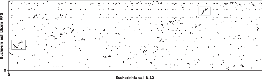
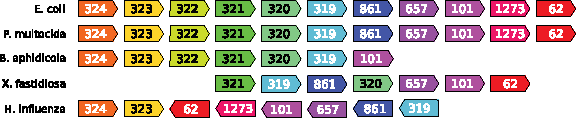
With the increasing availability of completely sequenced and assembled genomes, gene-order based comparisons of whole genomes have recently become an important field in comparative genomics. It is well known that genomes evolve not only on the level of nucleotide sequence but also by means of large-scale rearrangements operations, such as inversions and transpositions, as well as changes of the gene content. Focusing on this large-scale structure, genomes are usually modeled as strings of integers so that genes belonging to the same gene family are represented by the same integer. If no selective pressure was acting on whole genome evolution, gene order and gene content would randomize over time. In reality, we observe a low overall gene order conservation between species that is contrasted by a number of small, well-conserved segments, often referred to as gene clusters (Fig. 1).
Visualization of gene order conservation between the two γ-proteobacteria Escherichia coli (4183 genes) and Buchnera aphidicola (564 genes). The boxes indicate areas of conserved gene content/gene order.
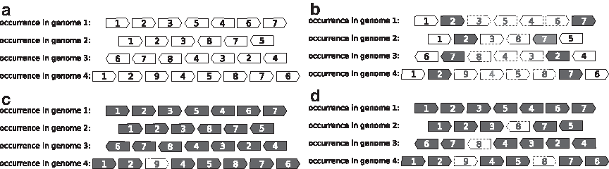
Such local aberrations from genome randomization are known to provide highly informative signals for functional analysis (Price et al., 2005; Rogozin et al., 2004; Wolf et al., 2001; Yanai et al., 2002; Huynen and Snel, 2000; Overbeek et al., 1999; Tamames et al., 1997). When comparing a large number of genomes, the identification of these structures can be a challenging task, as conservation patterns may be highly variable across species. Due to micro-rearrangements, gene order can vary across cluster occurrences, and due to gene insertions and gene losses, cluster occurrences may be interrupted by genes that do not belong to the cluster, and contain only a subset of the clustered genes. To cope with such variations, different approximate gene cluster models have been proposed in the last years. We briefly review the most common ones and illustrate their predictive power in Figure 2.
Approximate occurrences of an artificial gene cluster predicted under different gene cluster models. Gray-shaded genes belong to the predicted cluster; dotted genes indicate intermitting genes; the remaining genes are located outside the predicted cluster occurrences. (a) Using the common intervals based model, the cluster is not detected. Only for a subset of the genomes, parts of the cluster are detected, e.g., genes 1, 2, and 3 are clustered in genomes 1 and 2. (b) For a gap size of at least four, the max-gap approach clusters genes 2 and 7, the only ones present in all four occurrences. (c) Under the median gene cluster model, genes 1, 2, 3, 4, 5, 6, 7, and 8 form a cluster that underwent in total six gene losses, one gene insertion and one neutral gene duplication that are distributed over its four approximate occurrences. (d) The predicted median gene cluster has no reference occurrence, but the same approximate occurrences are reported when choosing the occurrence in genome 1 as reference. However, due to the absence of gene 8 there, three additional insertions are needed in the other occurrences.
One of the first formal gene cluster models are common intervals (Uno and Yagiura, 2000; Heber and Stoye, 2001a,b; Schmidt and Stoye, 2004; Didier et al., 2007; Didier, 2003), which allow for variable gene order and multiple gene copies within cluster occurrences, but not for differences in the set of contained genes. Due to this restriction, the computation of gene clusters under the common intervals model runs in polynomial time with respect to the maximum genome length n.
To represent more diverse conservation patterns, the so-called max-gap clusters (Bergeron et al., 2002; He and Goldwasser, 2005), also known as gene teams or homology teams, were developed. This widely used gene cluster model covers gene insertions but lacks a proper treatment of incomplete conservation of gene content. Its basic idea is to allow for an arbitrary number of gaps in every cluster occurrence, each up to a fixed length, that can be filled with intermitting genes. Gene losses are treated only indirectly: Any gene that is lost in a cluster occurrence is counted as an intermitting gene in those occurrences where it is still present. Therefore, the set of genes representing a gene cluster reduces to a minimal consensus: the genes that occur in all cluster occurrences. In consequence, it may become necessary to tolerate artificially high gap sizes to bridge seemingly intermitting genes. These phenomena are illustrated in Figure 2b. The asymptotic complexity of identifying max-gap clusters increases exponentially with the number of compared genomes, but practical running times were shown to be feasible (Ling et al., 2009).
To improve the treatment of gene losses, a number of set distance based models arose recently, for example, median gene clusters (Rahmann and Klau, 2006; Böcker et al., 2009), that extend the concept of common intervals towards approximate conservation of gene content. The basic idea is to define a maximum distance δ between a consensus gene set and its approximate occurrences which can be freely distributed over gene losses and insertions located anywhere in the approximate cluster occurrences. A reported gene cluster is not a minimal consensus but a set of genes that is optimized in the sense that the total distance to its approximate occurrences is minimized. In principle, this approach allows for the detection of gene clusters with diverse conservation patterns in a large number of genomes. Moreover, it is tolerant of errors in gene homology assignment which is an essential preprocessing step of most gene cluster detection tools. In some cases, it may even give hints at overlooked homologies; for example, in Figure 2c, the replacement of gene 3 with gene 9 in the fourth genome may suggest that the two genes are in fact unrecognized homologs. The cost for these generalizations is a search space that grows exponentially, either with the distance threshold δ (Rahmann and Klau, 2006) or the number of compared genomes k (Böcker et al., 2009). Practical computation times are feasible for many, but not all interesting parameter ranges. An alternative set distance based approach to gene cluster modeling are center gene clusters which were also briefly introduced in Böcker et al. (2009). This model differs from median gene clusters in the way the consensus gene set of approximate cluster occurrences is defined. It is based on minimizing pairwise distances, not the total distance. The complexity issue described above is not affected by this modification. In both models, the exponential search space is due to the optimality criterion imposed on the consensus gene set. However, if a gene cluster is not represented by an optimal consensus but a closely related set with a reference occurrence in the given genomes (i.e., one without intermitting or missing genes), the search space becomes polynomially bounded. An example of such a reference based gene cluster can be seen in Figure 2d. The computation of reference based conservation patterns was studied by Amir et al. (2007). However, it is possible to construct a counter example for which their graph-based, O(kn3 + output size) time and O(kn3) space, algorithm does not detect the complete solution set. (For details, see the Appendix of this article.)
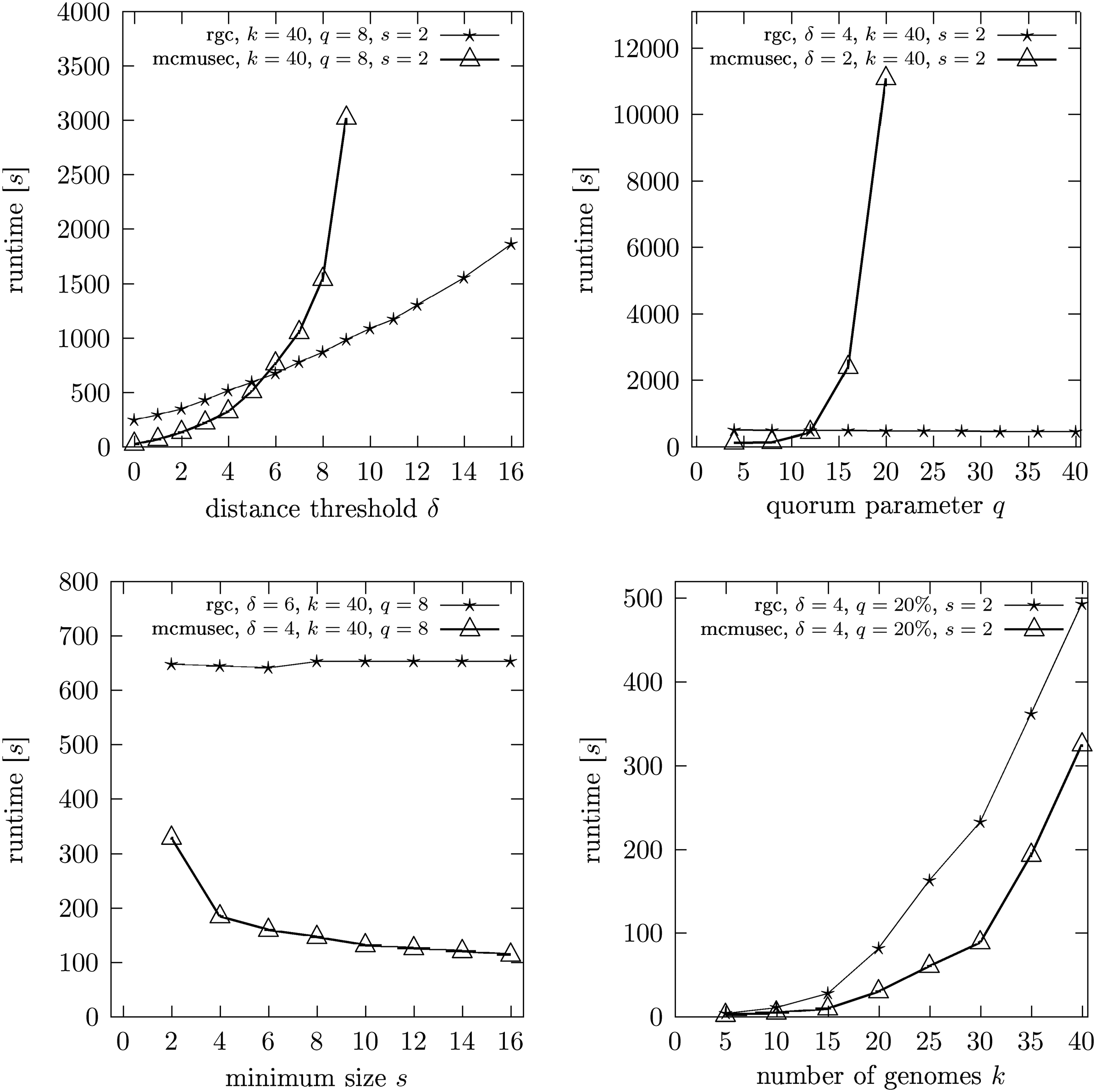
In this article, we show that the complete set of reference-based approximate gene cluster occurrences can be identified in time O(k2n2(δ + 1)2), δ ≪ n, using O(kn2) space. To assess the relevance of the reference-based gene cluster model and the performance of our algorithm, we compare it to the center gene cluster model and to mcmusec (Ling et al., 2009), the state-of-the-art approach to max-gap gene cluster computation.
2. Basic Definitions And Notation
We model a genome as a string over a finite alphabet \documentclass{aastex}\usepackage{amsbsy}\usepackage{amsfonts}\usepackage{amssymb}\usepackage{bm}\usepackage{mathrsfs}\usepackage{pifont}\usepackage{stmaryrd}\usepackage{textcomp}\usepackage{portland, xspace}\usepackage{amsmath, amsxtra}\pagestyle{empty}\DeclareMathSizes {10} {9} {7} {6}\begin{document}$$\Sigma = \{ 1, \ldots, \sigma \}$$\end{document} of gene family ids, such that genes belonging to the same homology family are represented by the same integer. Given a string S, we denote its length by |S| and refer to its ith character by S[i], 1 ≤ i ≤ |S|. We say that character \documentclass{aastex}\usepackage{amsbsy}\usepackage{amsfonts}\usepackage{amssymb}\usepackage{bm}\usepackage{mathrsfs}\usepackage{pifont}\usepackage{stmaryrd}\usepackage{textcomp}\usepackage{portland, xspace}\usepackage{amsmath, amsxtra}\pagestyle{empty}\DeclareMathSizes {10} {9} {7} {6}\begin{document}$$c \in \Sigma$$\end{document}occurs at position i in S if and only if S[i] = c. To capture the character content of S regardless of sequential arrangement and multiple character occurrences, we define the character set of S as \documentclass{aastex}\usepackage{amsbsy}\usepackage{amsfonts}\usepackage{amssymb}\usepackage{bm}\usepackage{mathrsfs}\usepackage{pifont}\usepackage{stmaryrd}\usepackage{textcomp}\usepackage{portland, xspace}\usepackage{amsmath, amsxtra}\pagestyle{empty}\DeclareMathSizes {10} {9} {7} {6}\begin{document}$${ \cal CS} (S) = \{ S [i] | 1 \leq i \leq | S | \}$$\end{document}. To simplify notation, we assume that a string S is extended on both ends by a terminal character \documentclass{aastex}\usepackage{amsbsy}\usepackage{amsfonts}\usepackage{amssymb}\usepackage{bm}\usepackage{mathrsfs}\usepackage{pifont}\usepackage{stmaryrd}\usepackage{textcomp}\usepackage{portland, xspace}\usepackage{amsmath, amsxtra}\pagestyle{empty}\DeclareMathSizes {10} {9} {7} {6}\begin{document}$$0 \notin \Sigma$$\end{document}, i.e. S[0] = S[|S| + 1] = 0. We define S[i, j] to be the substring of S that starts with its ith and ends with its jth character, 1 ≤ i ≤ j ≤ |S|. The corresponding index interval [i, j] is called a location of C ⊆ Σ if and only if \documentclass{aastex}\usepackage{amsbsy}\usepackage{amsfonts}\usepackage{amssymb}\usepackage{bm}\usepackage{mathrsfs}\usepackage{pifont}\usepackage{stmaryrd}\usepackage{textcomp}\usepackage{portland, xspace}\usepackage{amsmath, amsxtra}\pagestyle{empty}\DeclareMathSizes {10} {9} {7} {6}\begin{document}$$C = { \cal CS} (S [i, j])$$\end{document}. We distinguish different types of intervals in a string S. We call an interval [i, j] with j ≥ i left-maximal if \documentclass{aastex}\usepackage{amsbsy}\usepackage{amsfonts}\usepackage{amssymb}\usepackage{bm}\usepackage{mathrsfs}\usepackage{pifont}\usepackage{stmaryrd}\usepackage{textcomp}\usepackage{portland, xspace}\usepackage{amsmath, amsxtra}\pagestyle{empty}\DeclareMathSizes {10} {9} {7} {6}\begin{document}$$S [i - 1] \notin { \cal CS} (S [i, j])$$\end{document}, right-maximal if \documentclass{aastex}\usepackage{amsbsy}\usepackage{amsfonts}\usepackage{amssymb}\usepackage{bm}\usepackage{mathrsfs}\usepackage{pifont}\usepackage{stmaryrd}\usepackage{textcomp}\usepackage{portland, xspace}\usepackage{amsmath, amsxtra}\pagestyle{empty}\DeclareMathSizes {10} {9} {7} {6}\begin{document}$$S [j + 1] \notin { \cal CS} (S [i, j])$$\end{document} and maximal if it is both left- and right-maximal. Given a set of strings \documentclass{aastex}\usepackage{amsbsy}\usepackage{amsfonts}\usepackage{amssymb}\usepackage{bm}\usepackage{mathrsfs}\usepackage{pifont}\usepackage{stmaryrd}\usepackage{textcomp}\usepackage{portland, xspace}\usepackage{amsmath, amsxtra}\pagestyle{empty}\DeclareMathSizes {10} {9} {7} {6}\begin{document}$${ \cal S} = \{ S_1, \ldots, S_k \}$$\end{document}, k ≥ 2, we call a k-tuple of maximal intervals (\documentclass{aastex}\usepackage{amsbsy}\usepackage{amsfonts}\usepackage{amssymb}\usepackage{bm}\usepackage{mathrsfs}\usepackage{pifont}\usepackage{stmaryrd}\usepackage{textcomp}\usepackage{portland, xspace}\usepackage{amsmath, amsxtra}\pagestyle{empty}\DeclareMathSizes {10} {9} {7} {6}\begin{document}$$[i_1, j_1], \ldots, [i_k, j_k]$$\end{document}) common intervals of \documentclass{aastex}\usepackage{amsbsy}\usepackage{amsfonts}\usepackage{amssymb}\usepackage{bm}\usepackage{mathrsfs}\usepackage{pifont}\usepackage{stmaryrd}\usepackage{textcomp}\usepackage{portland, xspace}\usepackage{amsmath, amsxtra}\pagestyle{empty}\DeclareMathSizes {10} {9} {7} {6}\begin{document}$${ \cal S}$$\end{document} if and only if there is a C ⊆ Σ with:
\documentclass{aastex}\usepackage{amsbsy}\usepackage{amsfonts}\usepackage{amssymb}\usepackage{bm}\usepackage{mathrsfs}\usepackage{pifont}\usepackage{stmaryrd}\usepackage{textcomp}\usepackage{portland,xspace}\usepackage{amsmath,amsxtra}\pagestyle{empty}\DeclareMathSizes{10}{9}{7}{6}\begin{document}
\begin{align*}
C = { \cal CS} (S_1 [i_1, j_1]) = \ldots = { \cal CS} (S_k [i_k, j_k]).
\end{align*}
\end{document}
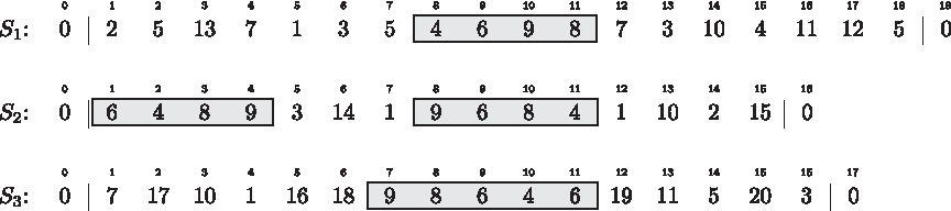
Such character sets correspond to clusters with perfectly conserved gene content. The above definitions are illustrated in Figure 3.
Each of the gray-shaded intervals is maximal and a location of the character set {4, 6, 8, 9}. The interval combinations ([8, 11], [1, 4], [7, 11]) and ([8, 11], [8, 11], [7, 11]) are common intervals of S1, S2 and S3.
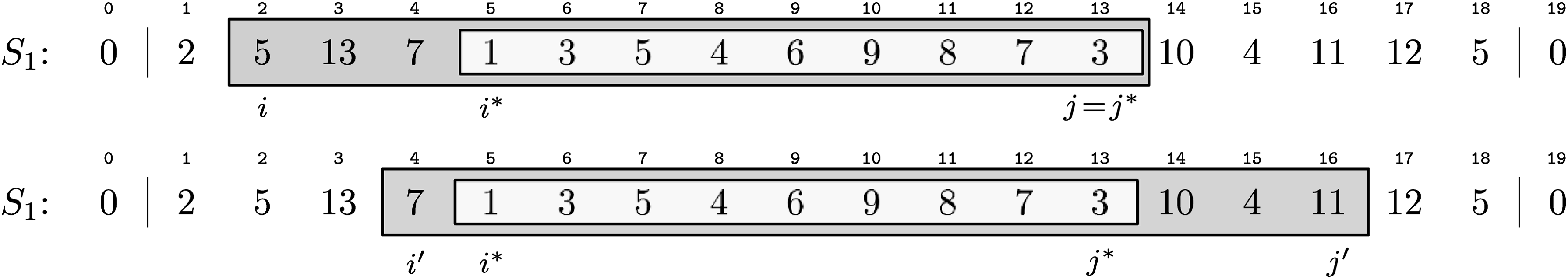
To quantify differences in the gene content of approximate gene cluster occurrences, we use the symmetric set distance, which defines the distance between two sets C and C′ as the cardinality of their symmetric difference: D(C, C′) = |C \C′| + |C′\C|. This measure constitutes a metric and therefore meets all intuitive notions of a distance measure such as validity of the triangle inequality. We extend the concept of character set locations towards approximate conservation: Given an integer δ ≥ 0, we say an interval [i, j] in a string S is a δ-location of a character set C if and only if \documentclass{aastex}\usepackage{amsbsy}\usepackage{amsfonts}\usepackage{amssymb}\usepackage{bm}\usepackage{mathrsfs}\usepackage{pifont}\usepackage{stmaryrd}\usepackage{textcomp}\usepackage{portland, xspace}\usepackage{amsmath, amsxtra}\pagestyle{empty}\DeclareMathSizes {10} {9} {7} {6}\begin{document}$$D (C, { \cal CS} (S [i, j])) \leq \delta$$\end{document} and \documentclass{aastex}\usepackage{amsbsy}\usepackage{amsfonts}\usepackage{amssymb}\usepackage{bm}\usepackage{mathrsfs}\usepackage{pifont}\usepackage{stmaryrd}\usepackage{textcomp}\usepackage{portland, xspace}\usepackage{amsmath, amsxtra}\pagestyle{empty}\DeclareMathSizes {10} {9} {7} {6}\begin{document}$$C \cap { \cal CS} (S [i, j]) \neq \emptyset$$\end{document}. The number of δ-locations of a C ⊆ Σ can grow quadratically with the string length n, even for δ = 0. This means that a gene cluster can not only have a large number of approximate occurrences, but also many overlapping ones. To avoid this redundancy, we introduce an optimality criterion for placing approximate cluster occurrences in a genomic area. Like in the definition of common intervals, we require interval maximality. Also, it is intuitive to forbid intervals that start/end next to a gene belonging to the gene cluster. Clearly, extending the interval to incorporate this gene yields a better approximate occurrence. Finally, it is not desirable to place an approximate occurrence such that one or both of its border genes do not belong to the gene cluster. Excluding such genes increases the compactness of the occurrence. However, to avoid conflict with interval maximality, we relax this condition slightly and allow such genes if they are copies of an intermitting gene occurring more centrally in the approximate occurrence. For an illustration of these concepts, assume we are given a gene set C = {1, 4, 8, 9}, the genomes shown in Figure 3 and a distance threshold δ = 2. Interval [8, 11] in genome S2 defines a δ-location of C, but this approximate occurrence can be improved by extending the borders to incorporate gene “1” on both ends. Interval [1, 4] also defines a non-optimal δ-location of C. It can be improved by excluding the left-most gene. For interval [7, 11] in genome S3 the compactness criterion conflicts with interval maximality. If we exclude gene “6” at position 11, we get a more compact occurrence, but the interval would be no longer maximal. Therefore, we prefer interval [7, 11] over [7, 10] when it comes to finding the optimal placement of C in this region of genome S3.
To formalize these optimality objectives, we define two subtypes of maximal intervals: Given a character set C, we say a maximal interval [i, j] in S with \documentclass{aastex}\usepackage{amsbsy}\usepackage{amsfonts}\usepackage{amssymb}\usepackage{bm}\usepackage{mathrsfs}\usepackage{pifont}\usepackage{stmaryrd}\usepackage{textcomp}\usepackage{portland, xspace}\usepackage{amsmath, amsxtra}\pagestyle{empty}\DeclareMathSizes {10} {9} {7} {6}\begin{document}$${ \cal CS} (S [i, j]) \cap C \neq \emptyset$$\end{document} is closed with respect to C, or C-closed for short, if and only if \documentclass{aastex}\usepackage{amsbsy}\usepackage{amsfonts}\usepackage{amssymb}\usepackage{bm}\usepackage{mathrsfs}\usepackage{pifont}\usepackage{stmaryrd}\usepackage{textcomp}\usepackage{portland, xspace}\usepackage{amsmath, amsxtra}\pagestyle{empty}\DeclareMathSizes {10} {9} {7} {6}\begin{document}$$S [i - 1] \notin C$$\end{document} and \documentclass{aastex}\usepackage{amsbsy}\usepackage{amsfonts}\usepackage{amssymb}\usepackage{bm}\usepackage{mathrsfs}\usepackage{pifont}\usepackage{stmaryrd}\usepackage{textcomp}\usepackage{portland, xspace}\usepackage{amsmath, amsxtra}\pagestyle{empty}\DeclareMathSizes {10} {9} {7} {6}\begin{document}$$S [j + 1] \notin C$$\end{document}. For the second subtype of maximal intervals, we define the left-most essential position i* of [i, j] with respect to C as the smallest index i′, i ≤ i′ ≤ j, such that \documentclass{aastex}\usepackage{amsbsy}\usepackage{amsfonts}\usepackage{amssymb}\usepackage{bm}\usepackage{mathrsfs}\usepackage{pifont}\usepackage{stmaryrd}\usepackage{textcomp}\usepackage{portland, xspace}\usepackage{amsmath, amsxtra}\pagestyle{empty}\DeclareMathSizes {10} {9} {7} {6}\begin{document}$$S [i^{ \prime}] \in C$$\end{document}. Analogously, we define the right-most essential position j* of [i, j] with respect to C as the largest index j′, i ≤ j′ ≤ j, such that \documentclass{aastex}\usepackage{amsbsy}\usepackage{amsfonts}\usepackage{amssymb}\usepackage{bm}\usepackage{mathrsfs}\usepackage{pifont}\usepackage{stmaryrd}\usepackage{textcomp}\usepackage{portland, xspace}\usepackage{amsmath, amsxtra}\pagestyle{empty}\DeclareMathSizes {10} {9} {7} {6}\begin{document}$$S [j^{ \prime}] \in C$$\end{document}. Interval [i*, j*] is called the C-essential subinterval of [i, j]. The characters at positions i* and j* are called left-most essential character, respectively right-most essential character, with respect to C. The second subtype of maximal intervals comprises all maximal intervals [i, j] with \documentclass{aastex}\usepackage{amsbsy}\usepackage{amsfonts}\usepackage{amssymb}\usepackage{bm}\usepackage{mathrsfs}\usepackage{pifont}\usepackage{stmaryrd}\usepackage{textcomp}\usepackage{portland, xspace}\usepackage{amsmath, amsxtra}\pagestyle{empty}\DeclareMathSizes {10} {9} {7} {6}\begin{document}$${ \cal CS} (S [i, j]) \cap C \neq \emptyset$$\end{document} for which \documentclass{aastex}\usepackage{amsbsy}\usepackage{amsfonts}\usepackage{amssymb}\usepackage{bm}\usepackage{mathrsfs}\usepackage{pifont}\usepackage{stmaryrd}\usepackage{textcomp}\usepackage{portland, xspace}\usepackage{amsmath, amsxtra}\pagestyle{empty}\DeclareMathSizes {10} {9} {7} {6}\begin{document}$${ \cal CS} (S [i, j]) = { \cal CS} (S [i^*, j^*])$$\end{document} holds. Maximal intervals fulfilling this property are called compact with respect to C or C-compact for short. If a maximal interval [i, j] is both closed and compact with respect to C, we call it optimal with respect to C, or C-optimal for short. A C-optimal δ-location of C is called an optimal δ-location. One can show that every region of approximate conservation is still detected:
Observation 1
Given an interval [i, j] in a string S and a character set C. If [i, j] is a δ-location of C for a δ ≥ 0, then there is also a δ-location that is C-optimal and contains the C-essential subinterval of [i, j].
Proof
We prove this by giving a construction algorithm: First, we identify the C-essential subinterval [i*, j*] which exists because \documentclass{aastex}\usepackage{amsbsy}\usepackage{amsfonts}\usepackage{amssymb}\usepackage{bm}\usepackage{mathrsfs}\usepackage{pifont}\usepackage{stmaryrd}\usepackage{textcomp}\usepackage{portland, xspace}\usepackage{amsmath, amsxtra}\pagestyle{empty}\DeclareMathSizes {10} {9} {7} {6}\begin{document}$${ \cal CS} (S [i, j]) \cap C \neq \emptyset$$\end{document} in each δ-location [i, j] of C. Then, we extend [i*, j*] on both ends to [i′, j′] until \documentclass{aastex}\usepackage{amsbsy}\usepackage{amsfonts}\usepackage{amssymb}\usepackage{bm}\usepackage{mathrsfs}\usepackage{pifont}\usepackage{stmaryrd}\usepackage{textcomp}\usepackage{portland, xspace}\usepackage{amsmath, amsxtra}\pagestyle{empty}\DeclareMathSizes {10} {9} {7} {6}\begin{document}$$S [i^{ \prime} - 1] \notin C \cup { \cal CS} (S [i^*, j^*])$$\end{document} and \documentclass{aastex}\usepackage{amsbsy}\usepackage{amsfonts}\usepackage{amssymb}\usepackage{bm}\usepackage{mathrsfs}\usepackage{pifont}\usepackage{stmaryrd}\usepackage{textcomp}\usepackage{portland, xspace}\usepackage{amsmath, amsxtra}\pagestyle{empty}\DeclareMathSizes {10} {9} {7} {6}\begin{document}$$S [j^{ \prime} + 1] \notin C \cup { \cal CS} (S [i^*, j^*])$$\end{document}. This happens at the latest when the extended string boundaries are reached, i.e., i′ = 1, respectively j′ = |S|. By construction such a [i′, j′] is C-optimal and contains [i*, j*]. It is also a δ-location of C: By definition \documentclass{aastex}\usepackage{amsbsy}\usepackage{amsfonts}\usepackage{amssymb}\usepackage{bm}\usepackage{mathrsfs}\usepackage{pifont}\usepackage{stmaryrd}\usepackage{textcomp}\usepackage{portland, xspace}\usepackage{amsmath, amsxtra}\pagestyle{empty}\DeclareMathSizes {10} {9} {7} {6}\begin{document}$$D ({ \cal CS} (S [i^*, j^*]), C) \leq D ({ \cal CS} (S [i, j]), C)$$\end{document} and in the following interval extension only two types of characters are added: those already contained in \documentclass{aastex}\usepackage{amsbsy}\usepackage{amsfonts}\usepackage{amssymb}\usepackage{bm}\usepackage{mathrsfs}\usepackage{pifont}\usepackage{stmaryrd}\usepackage{textcomp}\usepackage{portland, xspace}\usepackage{amsmath, amsxtra}\pagestyle{empty}\DeclareMathSizes {10} {9} {7} {6}\begin{document}$${ \cal CS} (S [i^*, j^*])$$\end{document}, which are neutral with respect to the distance to C, and elements from \documentclass{aastex}\usepackage{amsbsy}\usepackage{amsfonts}\usepackage{amssymb}\usepackage{bm}\usepackage{mathrsfs}\usepackage{pifont}\usepackage{stmaryrd}\usepackage{textcomp}\usepackage{portland, xspace}\usepackage{amsmath, amsxtra}\pagestyle{empty}\DeclareMathSizes {10} {9} {7} {6}\begin{document}$$C \setminus { \cal CS} (S [i^*, j^*])$$\end{document}, which reduce the distance. Therefore, also the distance constraint is met. ■
The construction used in the proof of Observation 1 is illustrated in Figure 4. Optimal δ-locations can still overlap, but compared to general δ-locations there is a tighter upper bound for their number:
Construction of the C-optimal interval [4, 16] from the interval [2, 13] via its C-essential subinterval [5, 13] for C = {1, 3, 4, 6, 8, 9, 10, 11}. The distance between C and \documentclass{aastex}\usepackage{amsbsy}\usepackage{amsfonts}\usepackage{amssymb}\usepackage{bm}\usepackage{mathrsfs}\usepackage{pifont}\usepackage{stmaryrd}\usepackage{textcomp}\usepackage{portland, xspace}\usepackage{amsmath, amsxtra}\pagestyle{empty}\DeclareMathSizes {10} {9} {7} {6}\begin{document}$${ \cal CS} (S_1 [2, 13])$$\end{document} equals 5 and decreases to 2 when [2, 13] is replaced by [4, 16].
Observation 2
The number of optimal δ-locations of a character set C ⊆ Σ in a string S of length n is in O(n(δ + 1)) for all δ ≥ 0.
Proof
We count how many optimal δ-locations of C can have the same left-most position a in S. For that purpose, we show that every two such intervals [a, b1] and [a, b2], b1 < b2, contain a different number of characters from Σ \ C. We have \documentclass{aastex}\usepackage{amsbsy}\usepackage{amsfonts}\usepackage{amssymb}\usepackage{bm}\usepackage{mathrsfs}\usepackage{pifont}\usepackage{stmaryrd}\usepackage{textcomp}\usepackage{portland, xspace}\usepackage{amsmath, amsxtra}\pagestyle{empty}\DeclareMathSizes {10} {9} {7} {6}\begin{document}$$S [b_1 + 1] \notin C$$\end{document} and \documentclass{aastex}\usepackage{amsbsy}\usepackage{amsfonts}\usepackage{amssymb}\usepackage{bm}\usepackage{mathrsfs}\usepackage{pifont}\usepackage{stmaryrd}\usepackage{textcomp}\usepackage{portland, xspace}\usepackage{amsmath, amsxtra}\pagestyle{empty}\DeclareMathSizes {10} {9} {7} {6}\begin{document}$$S [b_1 + 1] \notin { \cal CS} (S [a, b_1])$$\end{document}, while \documentclass{aastex}\usepackage{amsbsy}\usepackage{amsfonts}\usepackage{amssymb}\usepackage{bm}\usepackage{mathrsfs}\usepackage{pifont}\usepackage{stmaryrd}\usepackage{textcomp}\usepackage{portland, xspace}\usepackage{amsmath, amsxtra}\pagestyle{empty}\DeclareMathSizes {10} {9} {7} {6}\begin{document}$$S [b_1 + 1] \in { \cal CS} (S [a, b_2])$$\end{document}. However, it also holds that every \documentclass{aastex}\usepackage{amsbsy}\usepackage{amsfonts}\usepackage{amssymb}\usepackage{bm}\usepackage{mathrsfs}\usepackage{pifont}\usepackage{stmaryrd}\usepackage{textcomp}\usepackage{portland, xspace}\usepackage{amsmath, amsxtra}\pagestyle{empty}\DeclareMathSizes {10} {9} {7} {6}\begin{document}$$c \in{ \cal CS} (S [a, b_1]) \setminus C$$\end{document} is contained in \documentclass{aastex}\usepackage{amsbsy}\usepackage{amsfonts}\usepackage{amssymb}\usepackage{bm}\usepackage{mathrsfs}\usepackage{pifont}\usepackage{stmaryrd}\usepackage{textcomp}\usepackage{portland, xspace}\usepackage{amsmath, amsxtra}\pagestyle{empty}\DeclareMathSizes {10} {9} {7} {6}\begin{document}$${ \cal CS} (S [a, b_2])$$\end{document}. Therefore, the number of characters from Σ \ C cannot be the same in the two intervals. Moreover, a δ-location of C can have only between 0 and δ characters from Σ \ C. Thus, there are at most δ + 1 optimal δ-locations of C with left-most position a and O(n(δ + 1)) optimal δ-locations of C in the complete string. ■
We now have all the prerequisites to define the problems studied in this paper. At first, we study the detection of optimal δ-locations:
Problem 1
Given two strings S1and S2over an alphabet Σ and a distance threshold δ, find for each maximal [i, j] in S1all optimal δ-locations of\documentclass{aastex}\usepackage{amsbsy}\usepackage{amsfonts}\usepackage{amssymb}\usepackage{bm}\usepackage{mathrsfs}\usepackage{pifont}\usepackage{stmaryrd}\usepackage{textcomp}\usepackage{portland, xspace}\usepackage{amsmath, amsxtra}\pagestyle{empty}\DeclareMathSizes {10} {9} {7} {6}\begin{document}$${ \cal CS} (S_1 [i, j])$$\end{document}in S2.
For δ = 0, this problem is equivalent to common intervals detection. For reference-based approximate gene cluster detection in multiple genomes the definition can be extended as follows:
Problem 2
Given a set of strings\documentclass{aastex}\usepackage{amsbsy}\usepackage{amsfonts}\usepackage{amssymb}\usepackage{bm}\usepackage{mathrsfs}\usepackage{pifont}\usepackage{stmaryrd}\usepackage{textcomp}\usepackage{portland, xspace}\usepackage{amsmath, amsxtra}\pagestyle{empty}\DeclareMathSizes {10} {9} {7} {6}\begin{document}$${ \cal S} = \{ S_1, \ldots, S_k \}$$\end{document}over an alphabet Σ, a distance threshold δ and a quorum parameter q ≤ k, find each C ⊆ Σ with\documentclass{aastex}\usepackage{amsbsy}\usepackage{amsfonts}\usepackage{amssymb}\usepackage{bm}\usepackage{mathrsfs}\usepackage{pifont}\usepackage{stmaryrd}\usepackage{textcomp}\usepackage{portland, xspace}\usepackage{amsmath, amsxtra}\pagestyle{empty}\DeclareMathSizes {10} {9} {7} {6}\begin{document}$$C = { \cal CS} (S_{ \ell} [i_ \ell, j_ \ell])$$\end{document}for some 1 ≤ ℓ ≤ k, 1 ≤ iℓ ≤ jℓ ≤ |Sℓ| that has δ-locations in at least q different strings and report all its optimal δ-locations in\documentclass{aastex}\usepackage{amsbsy}\usepackage{amsfonts}\usepackage{amssymb}\usepackage{bm}\usepackage{mathrsfs}\usepackage{pifont}\usepackage{stmaryrd}\usepackage{textcomp}\usepackage{portland, xspace}\usepackage{amsmath, amsxtra}\pagestyle{empty}\DeclareMathSizes {10} {9} {7} {6}\begin{document}$$S_1, \ldots, S_k$$\end{document}.
We call character sets of the form of C conserved reference sets and their optimal δ-locations reference-based approximate common intervals.
3. Computation Of Optimal δ-Locations
The algorithm presented in the following adopts the basic search strategy of the Connecting Intervals (CI) Algorithm for the computation of common intervals (Schmidt and Stoye, 2004). Therefore, we begin with a short review of this algorithm.
3.1. The connecting intervals algorithm
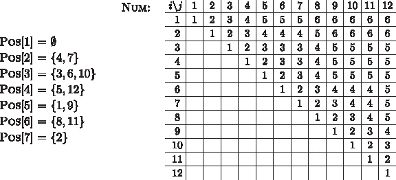
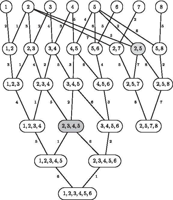
The CI Algorithm uses two static data structures that are computed in a preprocessing step: an array of length |Σ| called Pos that lists for each character \documentclass{aastex}\usepackage{amsbsy}\usepackage{amsfonts}\usepackage{amssymb}\usepackage{bm}\usepackage{mathrsfs}\usepackage{pifont}\usepackage{stmaryrd}\usepackage{textcomp}\usepackage{portland, xspace}\usepackage{amsmath, amsxtra}\pagestyle{empty}\DeclareMathSizes {10} {9} {7} {6}\begin{document}$$c \in \Sigma$$\end{document} its occurrences in S2 from left to right, and a |S2| × |S2| table named Num that stores for every interval in S2 how many different characters are contained, i.e., \documentclass{aastex}\usepackage{amsbsy}\usepackage{amsfonts}\usepackage{amssymb}\usepackage{bm}\usepackage{mathrsfs}\usepackage{pifont}\usepackage{stmaryrd}\usepackage{textcomp}\usepackage{portland, xspace}\usepackage{amsmath, amsxtra}\pagestyle{empty}\DeclareMathSizes {10} {9} {7} {6}\begin{document}$${ \sc Num} [i, j] = | { \cal CS} (S_2 [i, j]) |$$\end{document}. For an example, see Figure 5.
Example of data structures Pos and Num for alphabet Σ = {1, 2, 3, 4, 5, 6, 7} and two strings S1 = 1 2 4 6 4 3 1 5 6 2 and S2 = 5 7 3 2 4 3 2 6 5 3 6 4.
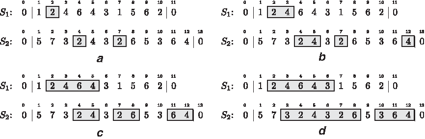
The basic idea of the CI Algorithm is that while going systematically through all maximal intervals [i, j] in S1, referred to as reference intervals in the following, one iteratively generates and extends marked intervals in S2 that consist only of characters occurring in the current reference character set\documentclass{aastex}\usepackage{amsbsy}\usepackage{amsfonts}\usepackage{amssymb}\usepackage{bm}\usepackage{mathrsfs}\usepackage{pifont}\usepackage{stmaryrd}\usepackage{textcomp}\usepackage{portland, xspace}\usepackage{amsmath, amsxtra}\pagestyle{empty}\DeclareMathSizes {10} {9} {7} {6}\begin{document}$${ \cal CS} (S_1 [i, j])$$\end{document} using array Pos for their identification. An example of this procedure is given in Figure 6.
Iterative generation of reference intervals in S1 for start position 2 and corresponding interval marking in S2 for S1 = 1 2 4 6 4 3 1 5 6 2 and S2 = 5 7 3 2 4 3 2 6 5 3 6 4.
Common intervals are retrieved by comparing the character content of \documentclass{aastex}\usepackage{amsbsy}\usepackage{amsfonts}\usepackage{amssymb}\usepackage{bm}\usepackage{mathrsfs}\usepackage{pifont}\usepackage{stmaryrd}\usepackage{textcomp}\usepackage{portland, xspace}\usepackage{amsmath, amsxtra}\pagestyle{empty}\DeclareMathSizes {10} {9} {7} {6}\begin{document}$${ \cal CS} (S_1 [i, j])$$\end{document} and the marked intervals in S2. Since by construction the character sets of the marked intervals are subsets of \documentclass{aastex}\usepackage{amsbsy}\usepackage{amsfonts}\usepackage{amssymb}\usepackage{bm}\usepackage{mathrsfs}\usepackage{pifont}\usepackage{stmaryrd}\usepackage{textcomp}\usepackage{portland, xspace}\usepackage{amsmath, amsxtra}\pagestyle{empty}\DeclareMathSizes {10} {9} {7} {6}\begin{document}$${ \cal CS} (S_1 [i, j])$$\end{document}, this can be tested by comparing their sizes, using the table Num, and the current size of \documentclass{aastex}\usepackage{amsbsy}\usepackage{amsfonts}\usepackage{amssymb}\usepackage{bm}\usepackage{mathrsfs}\usepackage{pifont}\usepackage{stmaryrd}\usepackage{textcomp}\usepackage{portland, xspace}\usepackage{amsmath, amsxtra}\pagestyle{empty}\DeclareMathSizes {10} {9} {7} {6}\begin{document}$${ \cal CS} (S_1 [i, j])$$\end{document}. Only those intervals in S2 that were extended by an occurrence of the most recent element of the reference character set need to be considered for this test. Other intervals do not contain this character and thus have a smaller character set. It can be shown that this algorithm detects all common intervals in time O(n2) using O(n2) space.
3.2. Extension of the connecting intervals algorithm
The changes necessary to the CI Algorithm to compute optimal δ-locations are presented together with the pseudocode given in Algorithm 1. The presented algorithm is a further development of the first step in the median gene cluster computation scheme where for a given δ only the existence of a δ-location is tested. To solve Problem 1, we need to enumerate all optimal δ-locations.
14: for each interval [lx + 1, ry − 1] with 1 ≤ x, y ≤ δ + 1 do
15: if [lx + 1, ry − 1] is an optimal δ-location and not contained in \documentclass{aastex}\usepackage{amsbsy}\usepackage{amsfonts}\usepackage{amssymb}\usepackage{bm}\usepackage{mathrsfs}\usepackage{pifont}\usepackage{stmaryrd}\usepackage{textcomp}\usepackage{portland, xspace}\usepackage{amsmath, amsxtra}\pagestyle{empty}\DeclareMathSizes {10} {9} {7} {6}\begin{document}$${ \cal C}$$\end{document}then
16: add [lx + 1, ry − 1] to \documentclass{aastex}\usepackage{amsbsy}\usepackage{amsfonts}\usepackage{amssymb}\usepackage{bm}\usepackage{mathrsfs}\usepackage{pifont}\usepackage{stmaryrd}\usepackage{textcomp}\usepackage{portland, xspace}\usepackage{amsmath, amsxtra}\pagestyle{empty}\DeclareMathSizes {10} {9} {7} {6}\begin{document}$${ \cal C}$$\end{document}
We adopt the iterative generation of reference intervals from the original CI Algorithm, where for a fixed i the maximal intervals starting at i are processed one after the other for increasing values of j (lines 1–7). Also the marking of intervals in S2 that consist only of characters from the current reference character set \documentclass{aastex}\usepackage{amsbsy}\usepackage{amsfonts}\usepackage{amssymb}\usepackage{bm}\usepackage{mathrsfs}\usepackage{pifont}\usepackage{stmaryrd}\usepackage{textcomp}\usepackage{portland, xspace}\usepackage{amsmath, amsxtra}\pagestyle{empty}\DeclareMathSizes {10} {9} {7} {6}\begin{document}$$C = { \cal CS} (S_1 [i, j])$$\end{document} (line 12) is useful for this purpose: Since approximate locations need to have character sets that intersect with C, these intervals are starting points for detecting C-optimal δ-locations. However, unlike with perfect locations, it is not sufficient to consider only recently extended maximal marked intervals. For δ > 0, intervals that are partially unmarked and/or contain no occurrence of c, the character most recently added to C, can as well be C-optimal δ-locations.
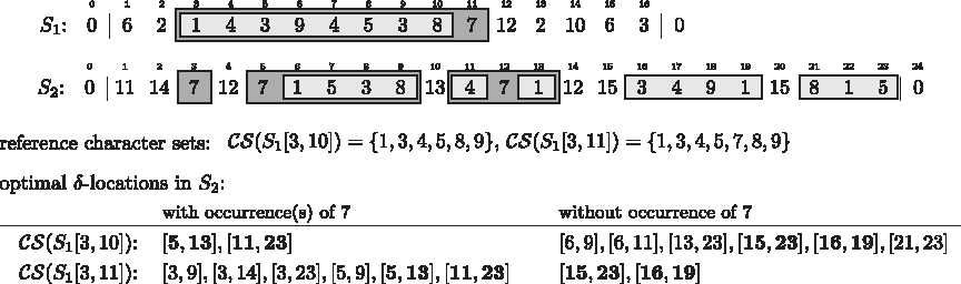
However, we observe that it is not necessary to compute optimal δ-locations from scratch for every reference character set. For a fixed left border i successive reference intervals [i, j′] and [i, j] with \documentclass{aastex}\usepackage{amsbsy}\usepackage{amsfonts}\usepackage{amssymb}\usepackage{bm}\usepackage{mathrsfs}\usepackage{pifont}\usepackage{stmaryrd}\usepackage{textcomp}\usepackage{portland, xspace}\usepackage{amsmath, amsxtra}\pagestyle{empty}\DeclareMathSizes {10} {9} {7} {6}\begin{document}$${ \cal CS} (S_1 [i, j]) = { \cal CS} (S_1 [i, j^{ \prime}]) \cup \{ c \}$$\end{document} can share some optimal δ-locations as the example in Figure 7 shows. Therefore, we store the optimal δ-locations of one reference character set in a list \documentclass{aastex}\usepackage{amsbsy}\usepackage{amsfonts}\usepackage{amssymb}\usepackage{bm}\usepackage{mathrsfs}\usepackage{pifont}\usepackage{stmaryrd}\usepackage{textcomp}\usepackage{portland, xspace}\usepackage{amsmath, amsxtra}\pagestyle{empty}\DeclareMathSizes {10} {9} {7} {6}\begin{document}$${ \cal C}$$\end{document} and test for the following reference character set which of these intervals can be inherited. Only in the case where the left border of the reference interval is shifted, \documentclass{aastex}\usepackage{amsbsy}\usepackage{amsfonts}\usepackage{amssymb}\usepackage{bm}\usepackage{mathrsfs}\usepackage{pifont}\usepackage{stmaryrd}\usepackage{textcomp}\usepackage{portland, xspace}\usepackage{amsmath, amsxtra}\pagestyle{empty}\DeclareMathSizes {10} {9} {7} {6}\begin{document}$${ \cal C}$$\end{document} is emptied as the generation of reference character sets starts anew (line 2). The optimal δ-locations that can be inherited to the next reference character set can be characterized as follows:
Optimal δ-locations of two successive reference character sets in two example strings S1 and S2 for distance threshold δ = 3. Shared optimal δ-locations are printed bold.
Observation 3
Let C, C′ ⊆ Σ with C = C′ ∪ {c} and \documentclass{aastex}\usepackage{amsbsy}\usepackage{amsfonts}\usepackage{amssymb}\usepackage{bm}\usepackage{mathrsfs}\usepackage{pifont}\usepackage{stmaryrd}\usepackage{textcomp}\usepackage{portland, xspace}\usepackage{amsmath, amsxtra}\pagestyle{empty}\DeclareMathSizes {10} {9} {7} {6}\begin{document}$$c \notin C^{ \prime}$$\end{document}. Every interval [a, b] in a string S over Σ that is an optimal δ-location of C′ is also an optimal δ-location of C if and only if either:
(i)\documentclass{aastex}\usepackage{amsbsy}\usepackage{amsfonts}\usepackage{amssymb}\usepackage{bm}\usepackage{mathrsfs}\usepackage{pifont}\usepackage{stmaryrd}\usepackage{textcomp}\usepackage{portland, xspace}\usepackage{amsmath, amsxtra}\pagestyle{empty}\DeclareMathSizes {10} {9} {7} {6}\begin{document}$$c \in { \cal CS} (S [a, b])$$\end{document}, or
(i) Since [a, b] is C′-optimal and contains an occurrence of c, it is C-optimal. Moreover, \documentclass{aastex}\usepackage{amsbsy}\usepackage{amsfonts}\usepackage{amssymb}\usepackage{bm}\usepackage{mathrsfs}\usepackage{pifont}\usepackage{stmaryrd}\usepackage{textcomp}\usepackage{portland, xspace}\usepackage{amsmath, amsxtra}\pagestyle{empty}\DeclareMathSizes {10} {9} {7} {6}\begin{document}$$D({ \cal CS} (S [a, b]), C) < D ({ \cal CS} (S [a, b]), C^{ \prime}) < \delta$$\end{document} holds. (ii) ⇒ : From [a, b] being C-closed and from \documentclass{aastex}\usepackage{amsbsy}\usepackage{amsfonts}\usepackage{amssymb}\usepackage{bm}\usepackage{mathrsfs}\usepackage{pifont}\usepackage{stmaryrd}\usepackage{textcomp}\usepackage{portland, xspace}\usepackage{amsmath, amsxtra}\pagestyle{empty}\DeclareMathSizes {10} {9} {7} {6}\begin{document}$$c \in C$$\end{document} follows directly that \documentclass{aastex}\usepackage{amsbsy}\usepackage{amsfonts}\usepackage{amssymb}\usepackage{bm}\usepackage{mathrsfs}\usepackage{pifont}\usepackage{stmaryrd}\usepackage{textcomp}\usepackage{portland, xspace}\usepackage{amsmath, amsxtra}\pagestyle{empty}\DeclareMathSizes {10} {9} {7} {6}\begin{document}$$S [a - 1] \notin C$$\end{document} and \documentclass{aastex}\usepackage{amsbsy}\usepackage{amsfonts}\usepackage{amssymb}\usepackage{bm}\usepackage{mathrsfs}\usepackage{pifont}\usepackage{stmaryrd}\usepackage{textcomp}\usepackage{portland, xspace}\usepackage{amsmath, amsxtra}\pagestyle{empty}\DeclareMathSizes {10} {9} {7} {6}\begin{document}$$S [b + 1] \notin C$$\end{document}. Furthermore, we have \documentclass{aastex}\usepackage{amsbsy}\usepackage{amsfonts}\usepackage{amssymb}\usepackage{bm}\usepackage{mathrsfs}\usepackage{pifont}\usepackage{stmaryrd}\usepackage{textcomp}\usepackage{portland, xspace}\usepackage{amsmath, amsxtra}\pagestyle{empty}\DeclareMathSizes {10} {9} {7} {6}\begin{document}$$D (C, { \cal CS} (S [a, b])) \leq \delta$$\end{document}. Removing a single character from C that is not contained in \documentclass{aastex}\usepackage{amsbsy}\usepackage{amsfonts}\usepackage{amssymb}\usepackage{bm}\usepackage{mathrsfs}\usepackage{pifont}\usepackage{stmaryrd}\usepackage{textcomp}\usepackage{portland, xspace}\usepackage{amsmath, amsxtra}\pagestyle{empty}\DeclareMathSizes {10} {9} {7} {6}\begin{document}$${ \cal CS} (S [a, b])$$\end{document} reduces the distance by one. Therefore, \documentclass{aastex}\usepackage{amsbsy}\usepackage{amsfonts}\usepackage{amssymb}\usepackage{bm}\usepackage{mathrsfs}\usepackage{pifont}\usepackage{stmaryrd}\usepackage{textcomp}\usepackage{portland, xspace}\usepackage{amsmath, amsxtra}\pagestyle{empty}\DeclareMathSizes {10} {9} {7} {6}\begin{document}$$D (C^{ \prime}, { \cal CS} (S [a, b])) < \delta$$\end{document} holds. ⇐ : It follows from c ≠ S[a − 1], c ≠ S[b + 1] and C = C′ ∪ {c} that [a, b] is C-optimal. Furthermore, we have \documentclass{aastex}\usepackage{amsbsy}\usepackage{amsfonts}\usepackage{amssymb}\usepackage{bm}\usepackage{mathrsfs}\usepackage{pifont}\usepackage{stmaryrd}\usepackage{textcomp}\usepackage{portland, xspace}\usepackage{amsmath, amsxtra}\pagestyle{empty}\DeclareMathSizes {10} {9} {7} {6}\begin{document}$$D (C^{ \prime}, { \cal CS} (S [a, b])) < \delta$$\end{document}. Adding a single character to C′ increases this distance by at most one so that it cannot exceed δ. Therefore, [a, b] is an optimal δ-location of C. ■
Testing the elements of \documentclass{aastex}\usepackage{amsbsy}\usepackage{amsfonts}\usepackage{amssymb}\usepackage{bm}\usepackage{mathrsfs}\usepackage{pifont}\usepackage{stmaryrd}\usepackage{textcomp}\usepackage{portland, xspace}\usepackage{amsmath, amsxtra}\pagestyle{empty}\DeclareMathSizes {10} {9} {7} {6}\begin{document}$${ \cal C}$$\end{document} for the conditions given in Observation 3, we can remove all non-inheritable intervals (line 9). Next, we show how we can compute the optimal δ-locations that cannot be inherited from the previous reference character set. These intervals are characterized as follows:
Observation 4
Let C, C′ ⊆ Σ with C = C′ ∪ {c} and\documentclass{aastex}\usepackage{amsbsy}\usepackage{amsfonts}\usepackage{amssymb}\usepackage{bm}\usepackage{mathrsfs}\usepackage{pifont}\usepackage{stmaryrd}\usepackage{textcomp}\usepackage{portland, xspace}\usepackage{amsmath, amsxtra}\pagestyle{empty}\DeclareMathSizes {10} {9} {7} {6}\begin{document}$$c \notin C^{ \prime}$$\end{document}. Every interval [a, b] in a string S over Σ that is an optimal δ-location of C is an optimal δ-location of C′ if and only if either:
(i)\documentclass{aastex}\usepackage{amsbsy}\usepackage{amsfonts}\usepackage{amssymb}\usepackage{bm}\usepackage{mathrsfs}\usepackage{pifont}\usepackage{stmaryrd}\usepackage{textcomp}\usepackage{portland, xspace}\usepackage{amsmath, amsxtra}\pagestyle{empty}\DeclareMathSizes {10} {9} {7} {6}\begin{document}$$c \notin { \cal CS} (S [a, b])$$\end{document}, or
(i) With [a, b] being C-optimal, S[a − 1] and S[b + 1] are not in C and therefore not in C′. Due to \documentclass{aastex}\usepackage{amsbsy}\usepackage{amsfonts}\usepackage{amssymb}\usepackage{bm}\usepackage{mathrsfs}\usepackage{pifont}\usepackage{stmaryrd}\usepackage{textcomp}\usepackage{portland, xspace}\usepackage{amsmath, amsxtra}\pagestyle{empty}\DeclareMathSizes {10} {9} {7} {6}\begin{document}$$c \notin { \cal CS} (S [a, b])$$\end{document}, [a, b] has the same left- and right-most essential positions with respect to C and C′. Thus, [a, b] is C′-optimal. Also, \documentclass{aastex}\usepackage{amsbsy}\usepackage{amsfonts}\usepackage{amssymb}\usepackage{bm}\usepackage{mathrsfs}\usepackage{pifont}\usepackage{stmaryrd}\usepackage{textcomp}\usepackage{portland, xspace}\usepackage{amsmath, amsxtra}\pagestyle{empty}\DeclareMathSizes {10} {9} {7} {6}\begin{document}$$D ({ \cal CS} (S [a, b]), C^{ \prime}) = D ({ \cal CS} (S [a, b]), C) - 1 \leq \delta - 1$$\end{document} holds. Hence, [a, b] is an optimal δ-location of C′.
(ii) ⇒ : From \documentclass{aastex}\usepackage{amsbsy}\usepackage{amsfonts}\usepackage{amssymb}\usepackage{bm}\usepackage{mathrsfs}\usepackage{pifont}\usepackage{stmaryrd}\usepackage{textcomp}\usepackage{portland, xspace}\usepackage{amsmath, amsxtra}\pagestyle{empty}\DeclareMathSizes {10} {9} {7} {6}\begin{document}$$D ({ \cal CS} (S [a, b]), C^{ \prime}) \leq \delta$$\end{document} follows \documentclass{aastex}\usepackage{amsbsy}\usepackage{amsfonts}\usepackage{amssymb}\usepackage{bm}\usepackage{mathrsfs}\usepackage{pifont}\usepackage{stmaryrd}\usepackage{textcomp}\usepackage{portland, xspace}\usepackage{amsmath, amsxtra}\pagestyle{empty}\DeclareMathSizes {10} {9} {7} {6}\begin{document}$$D ({ \cal CS} (S [a, b]), C) < \delta$$\end{document} because \documentclass{aastex}\usepackage{amsbsy}\usepackage{amsfonts}\usepackage{amssymb}\usepackage{bm}\usepackage{mathrsfs}\usepackage{pifont}\usepackage{stmaryrd}\usepackage{textcomp}\usepackage{portland, xspace}\usepackage{amsmath, amsxtra}\pagestyle{empty}\DeclareMathSizes {10} {9} {7} {6}\begin{document}$$c \in C$$\end{document} and \documentclass{aastex}\usepackage{amsbsy}\usepackage{amsfonts}\usepackage{amssymb}\usepackage{bm}\usepackage{mathrsfs}\usepackage{pifont}\usepackage{stmaryrd}\usepackage{textcomp}\usepackage{portland, xspace}\usepackage{amsmath, amsxtra}\pagestyle{empty}\DeclareMathSizes {10} {9} {7} {6}\begin{document}$$c \in { \cal CS} (S [a, b])$$\end{document}, but \documentclass{aastex}\usepackage{amsbsy}\usepackage{amsfonts}\usepackage{amssymb}\usepackage{bm}\usepackage{mathrsfs}\usepackage{pifont}\usepackage{stmaryrd}\usepackage{textcomp}\usepackage{portland, xspace}\usepackage{amsmath, amsxtra}\pagestyle{empty}\DeclareMathSizes {10} {9} {7} {6}\begin{document}$$c \notin C^{ \prime}$$\end{document}. Let pℓ and pr be left-most/right-most essential positions of [a, b] with respect to C′. Then S[pℓ] ≠ c, S[pr] ≠ c and ∃ p with pℓ < p < pr and S[p] = c due to C′-optimality and \documentclass{aastex}\usepackage{amsbsy}\usepackage{amsfonts}\usepackage{amssymb}\usepackage{bm}\usepackage{mathrsfs}\usepackage{pifont}\usepackage{stmaryrd}\usepackage{textcomp}\usepackage{portland, xspace}\usepackage{amsmath, amsxtra}\pagestyle{empty}\DeclareMathSizes {10} {9} {7} {6}\begin{document}$$c \in { \cal CS} (S [a, b])$$\end{document}. ⇐ : \documentclass{aastex}\usepackage{amsbsy}\usepackage{amsfonts}\usepackage{amssymb}\usepackage{bm}\usepackage{mathrsfs}\usepackage{pifont}\usepackage{stmaryrd}\usepackage{textcomp}\usepackage{portland, xspace}\usepackage{amsmath, amsxtra}\pagestyle{empty}\DeclareMathSizes {10} {9} {7} {6}\begin{document}$$D ({ \cal CS} (S [a, b]), C^{ \prime}) \leq \delta$$\end{document} holds, as \documentclass{aastex}\usepackage{amsbsy}\usepackage{amsfonts}\usepackage{amssymb}\usepackage{bm}\usepackage{mathrsfs}\usepackage{pifont}\usepackage{stmaryrd}\usepackage{textcomp}\usepackage{portland, xspace}\usepackage{amsmath, amsxtra}\pagestyle{empty}\DeclareMathSizes {10} {9} {7} {6}\begin{document}$$D ({ \cal CS} (S [a, b]), C^{ \prime}) = D ({ \cal CS} (S [a, b]), C) + 1$$\end{document} and \documentclass{aastex}\usepackage{amsbsy}\usepackage{amsfonts}\usepackage{amssymb}\usepackage{bm}\usepackage{mathrsfs}\usepackage{pifont}\usepackage{stmaryrd}\usepackage{textcomp}\usepackage{portland, xspace}\usepackage{amsmath, amsxtra}\pagestyle{empty}\DeclareMathSizes {10} {9} {7} {6}\begin{document}$$D ({ \cal CS} (S [a, b]), C) < \delta$$\end{document}. It follows from pℓ < p < pr that c is contained in the C′-essential subinterval of [a, b]. Since C and C′ differ only in c, [a, b] has to be C′-optimal. ■
An important consequence of this observation is that only intervals with an occurrence of c need to be considered for the computation of non-inheritable optimal δ-locations. Moreover, we can infer that there are exactly two types of them: intervals whose character set has exactly distance δ to C, and intervals with left-most and/or right-most essential character c that contain no “inner occurrences” of c, i.e., positions that are separated from both interval boundaries by characters from C other than c. Only these intervals need to be computed anew for every reference interval.
To detect these non-inheritable optimal δ-locations, we identify for each occurrence p of c in S2 all intervals around p that contain at most δ different unmarked characters. All other intervals either contain no occurrence of c or have a distance to C greater than δ. To find these intervals, we compute positions to the left and right of p with increasing numbers x, y ≥ 1 of unmarked characters (line 13):
lx = lx(p) = max({l | S2[l, p] contains x different unmarked characters} ∪ {0})
ry = ry(p) = min({r | S2[p, r] contains y different unmarked characters} ∪ {|S2| + 1}).
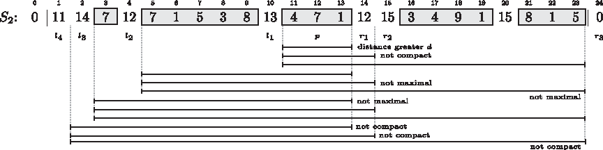
By definition, the substrings S2[lx + 1, ry − 1] contain at most x + y − 2 different characters not occurring in S1[i, j]. (The number is smaller if the same unmarked characters occur left and right of p.) Clearly, not all of them are C-optimal or fulfill the distance constraint, as the example in Figure 8 illustrates.
All intervals of the form [lx + 1, ry − 1] for p = 12, δ = 3. For intervals that are not an optimal δ-location of \documentclass{aastex}\usepackage{amsbsy}\usepackage{amsfonts}\usepackage{amssymb}\usepackage{bm}\usepackage{mathrsfs}\usepackage{pifont}\usepackage{stmaryrd}\usepackage{textcomp}\usepackage{portland, xspace}\usepackage{amsmath, amsxtra}\pagestyle{empty}\DeclareMathSizes {10} {9} {7} {6}\begin{document}$${ \cal CS} (S_1 [3, 11])$$\end{document}, the missing property is given.
But together, they form a superset of the C-optimal δ-locations around p. Thus, we only need to test every interval of the form [lx + 1, ry − 1] for being an optimal δ-location for the reference interval [i, j] and add it to \documentclass{aastex}\usepackage{amsbsy}\usepackage{amsfonts}\usepackage{amssymb}\usepackage{bm}\usepackage{mathrsfs}\usepackage{pifont}\usepackage{stmaryrd}\usepackage{textcomp}\usepackage{portland, xspace}\usepackage{amsmath, amsxtra}\pagestyle{empty}\DeclareMathSizes {10} {9} {7} {6}\begin{document}$${ \cal C}$$\end{document} if it passes this test and cannot be inherited from the previous reference character set (line 16).
It follows from Observations 3 and 4 that once all occurrences of c have been processed, \documentclass{aastex}\usepackage{amsbsy}\usepackage{amsfonts}\usepackage{amssymb}\usepackage{bm}\usepackage{mathrsfs}\usepackage{pifont}\usepackage{stmaryrd}\usepackage{textcomp}\usepackage{portland, xspace}\usepackage{amsmath, amsxtra}\pagestyle{empty}\DeclareMathSizes {10} {9} {7} {6}\begin{document}$${ \cal C}$$\end{document} contains all optimal δ-locations of C. To avoid that intervals with multiple occurrences of c are redundantly inserted, we add a rule by which only intervals in which p is the left-most occurrence of c are added to \documentclass{aastex}\usepackage{amsbsy}\usepackage{amsfonts}\usepackage{amssymb}\usepackage{bm}\usepackage{mathrsfs}\usepackage{pifont}\usepackage{stmaryrd}\usepackage{textcomp}\usepackage{portland, xspace}\usepackage{amsmath, amsxtra}\pagestyle{empty}\DeclareMathSizes {10} {9} {7} {6}\begin{document}$${ \cal C}$$\end{document}. From the previous considerations, it follows directly that the presented algorithm solves Problem 1.
3.3. Implementation details and data structures
Before we can analyze the time complexity of Algorithm 1, we need to have a closer look at some of the involved operations and the data structures that can be employed for their efficient implementation.
We begin with the identification of unmarked positions around the newly marked positions in S2 (line 13). An efficient approach to detect these positions was recently introduced in the context of median gene cluster computations (Böcker et al., 2009). It is based on two basic observations: First, the values lx and ry, 1 ≤ x, y ≤ δ + 1, can be precomputed for all positions p in S2 once the left border i of the next class of reference intervals [i, j], j ≥ i, is fixed. Second, the changes of these values between two successive positions i follow a simple pattern that allows for an efficient update. To see this pattern, we rank the characters in the strings S1[i,|S1|] and S2 by the order of their first occurrence in the concatenated string S1[i,|S1|]S2, initially for i = 1, and after each shift of the left border i. Such a bijection, Rank: \documentclass{aastex}\usepackage{amsbsy}\usepackage{amsfonts}\usepackage{amssymb}\usepackage{bm}\usepackage{mathrsfs}\usepackage{pifont}\usepackage{stmaryrd}\usepackage{textcomp}\usepackage{portland, xspace}\usepackage{amsmath, amsxtra}\pagestyle{empty}\DeclareMathSizes {10} {9} {7} {6}\begin{document}$${ \cal CS} (S_1 [i, | S_1 |] S_2) \to \{ 1, \ldots, | {\cal CS} (S_1 [i, | S_1 |] S_2) | \}$$\end{document}, can be generated in time O(n) which accumulates to O(n2) for a complete run of the algorithm. At the time the occurrences of c are marked in S2, the remaining unmarked characters c′ are such that Rank[c′] > Rank[c]. When i is shifted to i + 1, the rank of all characters occurring between i and the next occurrence of cold = S1[i] decreases by one while the rank of cold increases by the number of different characters between the two occurrences.
This leads to the following computation scheme: For i = 1, we simply scan the left and right neighborhood of each position p, look for the first δ + 1 different characters with a rank greater than Rank[S2[p]] and store these values in two δ × |S2| tables L and R such that L[p][x] = lx(p) and R[p][y] = ry(p) holds. Once i is shifted to i + 1, we update L and R separately for occurrences of cold = S1[i] and the remaining positions in S2. For occurrences of cold in S2 the entries in L and R can change completely due to a possibly large change of the rank of cold. We compute these values anew by going through S2 once from left to right and once from right to left remembering the last δ + 1 occurrences of characters with rank greater than the new rank of cold. If a character is read more than once, we only remember its latest occurrence. Once we reach an occurrence of cold, we fill the corresponding entries in L (respectively, R) with the remembered positions. For all other positions, the entries in L and R change only if the rank of the occurring character is smaller than the new rank of cold. For these positions, we need to check whether an occurrence of cold is close enough to become an entry in L and/or R. We test this by going through S2 once from left to right and once from right to left remembering the most recent occurrence of cold. Once we reach a position with a character of smaller rank than the new rank of cold, we go through its δ + 1 entries in L (respectively, R) and insert the remembered occurrence of cold at the appropriate position. For a complete run of Algorithm 1, the time spent on keeping L and R up to date accumulates to O(n2(δ + 1)).
Identification of left- and right-most essential positions
To test the candidate intervals [lx + 1, ry − 1] for being C-compact, we need to know their C-essential subintervals. We observe that the left-most essential position of an interval depends only on its left border and C while the right-most essential position depends only on the right border and C. Therefore, we need to determine for each lx and ry only one left-most (respectively right-most) essential position that is valid for all intervals with left border lx + 1, respectively right border ry − 1. We precompute and update these values parallel to the values of lx and ry using two additional tables L′ and R′ that are of the same format as L and R. In the following, we study only the computation and maintenance of L′. (The operations dealing with R′ are analogous.)
In terms of the character ranking, this task reads as follows: L′ needs to be maintained such that for all 1 ≤ p ≤ |S2| and 1 ≤ x ≤ δ + 1 entry L′[p][x] corresponds to the closest position to the right of L[p][x] that contains a character with rank smaller or equal to Rank[S2[p]]. We can initialize L′ for i = 1 at no extra cost during the initialization of L which involves a scan of the neighborhood of each position in S2. The update of L′ at positions p with S2[p] = cold is also straight-forward: During the scan of S2 for updating L, we track not only the last δ + 1 non-redundant occurrences of characters with rank greater than Rank[cold] but also for each of them the next position with rank at most Rank[cold]. We find such a position at the latest when we reach p. Therefore, all entries L′[p][x] for S2[p] = cold are set during this process.
For all other p, the entries L′[p][x] can only change if Rank[cold] > Rank[S2[p]]. To update L′ at these positions, we precompute for all occurrences of cold the δ + 1 next positions to the right with strictly decreasing rank lower than Rank[cold], referred to as lower ranked neighbors in the following. These positions can be identified for all occurrences of cold in a single scan of S2 which takes time O(nδ). (Details are left to the reader.) Then we check for each p that is not an occurrence of cold every L′[p][x] for being an occurrence of cold, and replace each L′[p][x] for which this is the case by the first lower ranked neighbor of L′[p][x] that has rank at most Rank[S2[p]]. We always find such a position among the lower ranked neighbors of L′[p][x], because there can occur no more than δ different characters with rank greater than δ between L[p][x] and p. The time spent on the complete update process of L′ is in O(nδ) which accumulates to O(n2δ) for a complete run of the algorithm. For symmetry reasons, the same is true for R′. The space consumption of L′ and R′ is in O(nδ).
Testing intervals for being optimal δ-locations
Next, we show how a candidate interval [lx + 1, ry − 1] can be tested for being an optimal δ-location of C (line 15). First, we test for interval maximality which is given if and only if there are no occurrences of S2[lx] and S2[ry] in S2[lx + 1, ry − 1]. This test can be done in constant time if we compute in a preprocessing for every position p in S2 the next and previous occurrence of S2[p] in S2 and store this information in two static arrays of length |S2|. Every maximal interval of the form [lx + 1, ry − 1] is automatically C-closed, because neither S2[lx] nor S2[ry] can be contained in C. C-compactness can be tested in constant time by comparing the entries in Num for [lx + 1, ry − 1] and its C-essential subinterval. To test the distance constraint, we compute \documentclass{aastex}\usepackage{amsbsy}\usepackage{amsfonts}\usepackage{amssymb}\usepackage{bm}\usepackage{mathrsfs}\usepackage{pifont}\usepackage{stmaryrd}\usepackage{textcomp}\usepackage{portland, xspace}\usepackage{amsmath, amsxtra}\pagestyle{empty}\DeclareMathSizes {10} {9} {7} {6}\begin{document}$$D ({ \cal CS} (S_1 [i, j]), { \cal CS} (S_2 [l_x + 1, r_y - 1]))$$\end{document}. This is equal to \documentclass{aastex}\usepackage{amsbsy}\usepackage{amsfonts}\usepackage{amssymb}\usepackage{bm}\usepackage{mathrsfs}\usepackage{pifont}\usepackage{stmaryrd}\usepackage{textcomp}\usepackage{portland, xspace}\usepackage{amsmath, amsxtra}\pagestyle{empty}\DeclareMathSizes {10} {9} {7} {6}\begin{document}$$| C | - | { \cal CS} (S_2 [l_x + 1, r_y - 1]) |$$\end{document} plus twice the number of different unmarked characters in S2[lx + 1, ry − 1]. \documentclass{aastex}\usepackage{amsbsy}\usepackage{amsfonts}\usepackage{amssymb}\usepackage{bm}\usepackage{mathrsfs}\usepackage{pifont}\usepackage{stmaryrd}\usepackage{textcomp}\usepackage{portland, xspace}\usepackage{amsmath, amsxtra}\pagestyle{empty}\DeclareMathSizes {10} {9} {7} {6}\begin{document}$$| { \cal CS} (S_2 [l_x + 1, r_y - 1]) |$$\end{document} can be looked up in Num. Also the value of |C| is directly available if it is tracked during reference interval generation. If we do a systematic enumeration of candidate intervals [lx + 1, ry − 1], we can track also the number of unmarked characters at no extra cost, and the complete distance computation can be performed in constant time. Finally, we need to test whether [lx + 1, ry − 1] is already contained in \documentclass{aastex}\usepackage{amsbsy}\usepackage{amsfonts}\usepackage{amssymb}\usepackage{bm}\usepackage{mathrsfs}\usepackage{pifont}\usepackage{stmaryrd}\usepackage{textcomp}\usepackage{portland, xspace}\usepackage{amsmath, amsxtra}\pagestyle{empty}\DeclareMathSizes {10} {9} {7} {6}\begin{document}$${ \cal C}$$\end{document}. Rather than testing condition (ii) of Observation 4, we generate first a separate list of the newly detected C-optimal δ-locations and then merge it with \documentclass{aastex}\usepackage{amsbsy}\usepackage{amsfonts}\usepackage{amssymb}\usepackage{bm}\usepackage{mathrsfs}\usepackage{pifont}\usepackage{stmaryrd}\usepackage{textcomp}\usepackage{portland, xspace}\usepackage{amsmath, amsxtra}\pagestyle{empty}\DeclareMathSizes {10} {9} {7} {6}\begin{document}$${ \cal C}$$\end{document}. This can be done efficiently if both lists are sorted based on the index positions of their elements, i.e., [a1, b1] occurs before [a2, b2] if and only if a1 < a2 or a1 = a2 and b1 < b2. We get such a sorting automatically if the occurrences of c in S2 and the corresponding [lx + 1, ry − 1] are always processed from left to right.
The second step where intervals are tested for being optimal δ-locations is in line 9 of Algorithm 1. To identify intervals in \documentclass{aastex}\usepackage{amsbsy}\usepackage{amsfonts}\usepackage{amssymb}\usepackage{bm}\usepackage{mathrsfs}\usepackage{pifont}\usepackage{stmaryrd}\usepackage{textcomp}\usepackage{portland, xspace}\usepackage{amsmath, amsxtra}\pagestyle{empty}\DeclareMathSizes {10} {9} {7} {6}\begin{document}$${ \cal C}$$\end{document} that contain an occurrence of c, we perform a combined iteration through \documentclass{aastex}\usepackage{amsbsy}\usepackage{amsfonts}\usepackage{amssymb}\usepackage{bm}\usepackage{mathrsfs}\usepackage{pifont}\usepackage{stmaryrd}\usepackage{textcomp}\usepackage{portland, xspace}\usepackage{amsmath, amsxtra}\pagestyle{empty}\DeclareMathSizes {10} {9} {7} {6}\begin{document}$${ \cal C}$$\end{document} and Pos[c]. We iterate for the first occurrence p of c through \documentclass{aastex}\usepackage{amsbsy}\usepackage{amsfonts}\usepackage{amssymb}\usepackage{bm}\usepackage{mathrsfs}\usepackage{pifont}\usepackage{stmaryrd}\usepackage{textcomp}\usepackage{portland, xspace}\usepackage{amsmath, amsxtra}\pagestyle{empty}\DeclareMathSizes {10} {9} {7} {6}\begin{document}$${ \cal C}$$\end{document} as long as we read elements [a, b] with a ≤ p. We test for each of them whether b ≥ p holds and, if this is the case, whether the interval contains an occurrence of c. As soon as we reach an element with a > p, we replace p by the next occurrence of c that is not located left of a and go on with the testing of the elements of \documentclass{aastex}\usepackage{amsbsy}\usepackage{amsfonts}\usepackage{amssymb}\usepackage{bm}\usepackage{mathrsfs}\usepackage{pifont}\usepackage{stmaryrd}\usepackage{textcomp}\usepackage{portland, xspace}\usepackage{amsmath, amsxtra}\pagestyle{empty}\DeclareMathSizes {10} {9} {7} {6}\begin{document}$${ \cal C}$$\end{document} until the end of either Pos[c] or \documentclass{aastex}\usepackage{amsbsy}\usepackage{amsfonts}\usepackage{amssymb}\usepackage{bm}\usepackage{mathrsfs}\usepackage{pifont}\usepackage{stmaryrd}\usepackage{textcomp}\usepackage{portland, xspace}\usepackage{amsmath, amsxtra}\pagestyle{empty}\DeclareMathSizes {10} {9} {7} {6}\begin{document}$${ \cal C}$$\end{document} is reached. For the intervals that contain no occurrence of c, condition (ii) of Observation 3 can be tested in constant time if we track for each interval the distance between its character set and the current C. To achieve this, we remember the initial distance when the element is added to \documentclass{aastex}\usepackage{amsbsy}\usepackage{amsfonts}\usepackage{amssymb}\usepackage{bm}\usepackage{mathrsfs}\usepackage{pifont}\usepackage{stmaryrd}\usepackage{textcomp}\usepackage{portland, xspace}\usepackage{amsmath, amsxtra}\pagestyle{empty}\DeclareMathSizes {10} {9} {7} {6}\begin{document}$${ \cal C}$$\end{document} an increment it by one each time it does not contain an occurrence of the recent c.
3.4. Complexity analysis
We now have all prerequisites to analyze the complexity of Algorithm 1. It follows from the analysis of the CI Algorithm that the generation of reference intervals in S1 and the marking of character occurrences in S2 is in O(n2). The first interesting step in Algorithm 1 is the iteration through \documentclass{aastex}\usepackage{amsbsy}\usepackage{amsfonts}\usepackage{amssymb}\usepackage{bm}\usepackage{mathrsfs}\usepackage{pifont}\usepackage{stmaryrd}\usepackage{textcomp}\usepackage{portland, xspace}\usepackage{amsmath, amsxtra}\pagestyle{empty}\DeclareMathSizes {10} {9} {7} {6}\begin{document}$${ \cal C}$$\end{document} to remove intervals that are not an optimal δ-location of the new reference character set (lines 8–10). The complete cost for the combined iterations through \documentclass{aastex}\usepackage{amsbsy}\usepackage{amsfonts}\usepackage{amssymb}\usepackage{bm}\usepackage{mathrsfs}\usepackage{pifont}\usepackage{stmaryrd}\usepackage{textcomp}\usepackage{portland, xspace}\usepackage{amsmath, amsxtra}\pagestyle{empty}\DeclareMathSizes {10} {9} {7} {6}\begin{document}$${ \cal C}$$\end{document} and Pos[c] is \documentclass{aastex}\usepackage{amsbsy}\usepackage{amsfonts}\usepackage{amssymb}\usepackage{bm}\usepackage{mathrsfs}\usepackage{pifont}\usepackage{stmaryrd}\usepackage{textcomp}\usepackage{portland, xspace}\usepackage{amsmath, amsxtra}\pagestyle{empty}\DeclareMathSizes {10} {9} {7} {6}\begin{document}$$O (n^2 + \sum \nolimits_{i \leq j} | { \cal C}_{i, j} |)$$\end{document}, where \documentclass{aastex}\usepackage{amsbsy}\usepackage{amsfonts}\usepackage{amssymb}\usepackage{bm}\usepackage{mathrsfs}\usepackage{pifont}\usepackage{stmaryrd}\usepackage{textcomp}\usepackage{portland, xspace}\usepackage{amsmath, amsxtra}\pagestyle{empty}\DeclareMathSizes {10} {9} {7} {6}\begin{document}$${ \cal C}_{i, j} = { \cal C}$$\end{document} at the time when reference interval [i, j] has been processed after line 22 of Algorithm 1. The first summand is due to the fact that every \documentclass{aastex}\usepackage{amsbsy}\usepackage{amsfonts}\usepackage{amssymb}\usepackage{bm}\usepackage{mathrsfs}\usepackage{pifont}\usepackage{stmaryrd}\usepackage{textcomp}\usepackage{portland, xspace}\usepackage{amsmath, amsxtra}\pagestyle{empty}\DeclareMathSizes {10} {9} {7} {6}\begin{document}$$c \in \Sigma$$\end{document} is O(n) times the most recent element in C and \documentclass{aastex}\usepackage{amsbsy}\usepackage{amsfonts}\usepackage{amssymb}\usepackage{bm}\usepackage{mathrsfs}\usepackage{pifont}\usepackage{stmaryrd}\usepackage{textcomp}\usepackage{portland, xspace}\usepackage{amsmath, amsxtra}\pagestyle{empty}\DeclareMathSizes {10} {9} {7} {6}\begin{document}$$n \cdot \sum \nolimits_{c \in \Sigma} | { \sc Pos} [c] | = n^2$$\end{document}, while the second summand stands for the combined length of \documentclass{aastex}\usepackage{amsbsy}\usepackage{amsfonts}\usepackage{amssymb}\usepackage{bm}\usepackage{mathrsfs}\usepackage{pifont}\usepackage{stmaryrd}\usepackage{textcomp}\usepackage{portland, xspace}\usepackage{amsmath, amsxtra}\pagestyle{empty}\DeclareMathSizes {10} {9} {7} {6}\begin{document}$${ \cal C}$$\end{document} over all O(n2) iterations through \documentclass{aastex}\usepackage{amsbsy}\usepackage{amsfonts}\usepackage{amssymb}\usepackage{bm}\usepackage{mathrsfs}\usepackage{pifont}\usepackage{stmaryrd}\usepackage{textcomp}\usepackage{portland, xspace}\usepackage{amsmath, amsxtra}\pagestyle{empty}\DeclareMathSizes {10} {9} {7} {6}\begin{document}$${ \cal C}$$\end{document} in line 8. As all elements of \documentclass{aastex}\usepackage{amsbsy}\usepackage{amsfonts}\usepackage{amssymb}\usepackage{bm}\usepackage{mathrsfs}\usepackage{pifont}\usepackage{stmaryrd}\usepackage{textcomp}\usepackage{portland, xspace}\usepackage{amsmath, amsxtra}\pagestyle{empty}\DeclareMathSizes {10} {9} {7} {6}\begin{document}$${ \cal C}$$\end{document} are optimal δ-locations of the previous reference character set, and since there are in total O(n2) reference intervals, it follows from Observation 1 that \documentclass{aastex}\usepackage{amsbsy}\usepackage{amsfonts}\usepackage{amssymb}\usepackage{bm}\usepackage{mathrsfs}\usepackage{pifont}\usepackage{stmaryrd}\usepackage{textcomp}\usepackage{portland, xspace}\usepackage{amsmath, amsxtra}\pagestyle{empty}\DeclareMathSizes {10} {9} {7} {6}\begin{document}$$\sum \nolimits_{i \leq j} | { \cal C}_{i, j} | \in O (n^3 (\delta + 1))$$\end{document}. We will derive a better bound later.
The next step of the algorithm is the computation of the non-inherited optimal δ-locations (lines 11–19). Every position p in S2 gets at most O(n) times newly marked, such that in total the for-loop in line 11 is executed O(n2) times. Using tables L and R, the unmarked positions \documentclass{aastex}\usepackage{amsbsy}\usepackage{amsfonts}\usepackage{amssymb}\usepackage{bm}\usepackage{mathrsfs}\usepackage{pifont}\usepackage{stmaryrd}\usepackage{textcomp}\usepackage{portland, xspace}\usepackage{amsmath, amsxtra}\pagestyle{empty}\DeclareMathSizes {10} {9} {7} {6}\begin{document}$$l_1, \ldots, l_{ \delta + 1}$$\end{document} and \documentclass{aastex}\usepackage{amsbsy}\usepackage{amsfonts}\usepackage{amssymb}\usepackage{bm}\usepackage{mathrsfs}\usepackage{pifont}\usepackage{stmaryrd}\usepackage{textcomp}\usepackage{portland, xspace}\usepackage{amsmath, amsxtra}\pagestyle{empty}\DeclareMathSizes {10} {9} {7} {6}\begin{document}$$r_1, \ldots, r_{ \delta + 1}$$\end{document} are immediately available. As we have seen above, the precomputation and maintenance of these data structures is in time O(n2(δ + 1)). It follows the processing of candidate intervals of the form [lx + 1, ry − 1]. For each occurrence p, there are O((δ + 1)2) many of these intervals, while there are |Pos[c]| many occurrences of each c in S2. With every position p in S2 being marked at most n times, \documentclass{aastex}\usepackage{amsbsy}\usepackage{amsfonts}\usepackage{amssymb}\usepackage{bm}\usepackage{mathrsfs}\usepackage{pifont}\usepackage{stmaryrd}\usepackage{textcomp}\usepackage{portland, xspace}\usepackage{amsmath, amsxtra}\pagestyle{empty}\DeclareMathSizes {10} {9} {7} {6}\begin{document}$$O (n \cdot \sum \nolimits_{c \in \Sigma} (| { \sc Pos} [c] | \cdot (\delta + 1) ^2)) = O (n^2 (\delta + 1) ^2)$$\end{document} intervals are considered during the complete run of Algorithm 1. Using the data structures described above, testing a single candidate for being an optimal δ-location of C takes constant time. Finally, the list of new optimal δ-locations is merged with \documentclass{aastex}\usepackage{amsbsy}\usepackage{amsfonts}\usepackage{amssymb}\usepackage{bm}\usepackage{mathrsfs}\usepackage{pifont}\usepackage{stmaryrd}\usepackage{textcomp}\usepackage{portland, xspace}\usepackage{amsmath, amsxtra}\pagestyle{empty}\DeclareMathSizes {10} {9} {7} {6}\begin{document}$${ \cal C}$$\end{document}. As both lists are sorted, the time spent on this operation equals the length of the new list plus the length of \documentclass{aastex}\usepackage{amsbsy}\usepackage{amsfonts}\usepackage{amssymb}\usepackage{bm}\usepackage{mathrsfs}\usepackage{pifont}\usepackage{stmaryrd}\usepackage{textcomp}\usepackage{portland, xspace}\usepackage{amsmath, amsxtra}\pagestyle{empty}\DeclareMathSizes {10} {9} {7} {6}\begin{document}$${ \cal C}$$\end{document}. Since all elements of \documentclass{aastex}\usepackage{amsbsy}\usepackage{amsfonts}\usepackage{amssymb}\usepackage{bm}\usepackage{mathrsfs}\usepackage{pifont}\usepackage{stmaryrd}\usepackage{textcomp}\usepackage{portland, xspace}\usepackage{amsmath, amsxtra}\pagestyle{empty}\DeclareMathSizes {10} {9} {7} {6}\begin{document}$${ \cal C}$$\end{document} are optimal δ-locations of the current C, this accumulates to \documentclass{aastex}\usepackage{amsbsy}\usepackage{amsfonts}\usepackage{amssymb}\usepackage{bm}\usepackage{mathrsfs}\usepackage{pifont}\usepackage{stmaryrd}\usepackage{textcomp}\usepackage{portland, xspace}\usepackage{amsmath, amsxtra}\pagestyle{empty}\DeclareMathSizes {10} {9} {7} {6}\begin{document}$$O (\sum \nolimits_{i \leq j} | { \cal C}_{i, j} | + n^2 (\delta + 1) ^2)$$\end{document} for the complete run of the algorithm.
To find a tighter bound for \documentclass{aastex}\usepackage{amsbsy}\usepackage{amsfonts}\usepackage{amssymb}\usepackage{bm}\usepackage{mathrsfs}\usepackage{pifont}\usepackage{stmaryrd}\usepackage{textcomp}\usepackage{portland, xspace}\usepackage{amsmath, amsxtra}\pagestyle{empty}\DeclareMathSizes {10} {9} {7} {6}\begin{document}$$\sum \nolimits_{i \leq j} | { \cal C}_{i, j} |$$\end{document}, we need to estimate how many intervals are added to \documentclass{aastex}\usepackage{amsbsy}\usepackage{amsfonts}\usepackage{amssymb}\usepackage{bm}\usepackage{mathrsfs}\usepackage{pifont}\usepackage{stmaryrd}\usepackage{textcomp}\usepackage{portland, xspace}\usepackage{amsmath, amsxtra}\pagestyle{empty}\DeclareMathSizes {10} {9} {7} {6}\begin{document}$${ \cal C}$$\end{document} in total and how long they can persist in \documentclass{aastex}\usepackage{amsbsy}\usepackage{amsfonts}\usepackage{amssymb}\usepackage{bm}\usepackage{mathrsfs}\usepackage{pifont}\usepackage{stmaryrd}\usepackage{textcomp}\usepackage{portland, xspace}\usepackage{amsmath, amsxtra}\pagestyle{empty}\DeclareMathSizes {10} {9} {7} {6}\begin{document}$${ \cal C}$$\end{document}. We can infer from Observation 4 that there are exactly two types of optimal δ-locations [a, b] that can not be inherited from the previous reference interval: the first type are intervals having exactly distance δ to C, and the second type are intervals with left-most and/or right-most essential character c that contain no “inner occurrences” of c, i.e., positions that are separated from both interval boundaries by characters from C other than c.
Non-inherited optimal δ-locations of the second type are necessarily either of the form [lx + 1, r1 − 1] or [l1 + 1, ry − 1]. Only such intervals can be C-optimal intervals with right-most essential position p, respectively, left-most essential position p. Since there are only δ + 1 many values of both, x and y, for every newly marked position, only O(δ + 1) many of these intervals exist. Each of them can persist in \documentclass{aastex}\usepackage{amsbsy}\usepackage{amsfonts}\usepackage{amssymb}\usepackage{bm}\usepackage{mathrsfs}\usepackage{pifont}\usepackage{stmaryrd}\usepackage{textcomp}\usepackage{portland, xspace}\usepackage{amsmath, amsxtra}\pagestyle{empty}\DeclareMathSizes {10} {9} {7} {6}\begin{document}$${ \cal C}$$\end{document} for at most O(δ + 1) iterations of the algorithm. Each time, either the new character of the reference character set is present in the interval which can happen at most δ times, otherwise the distance would have been above δ in the beginning, or the new character is not present. The latter can also happen at most δ times. Afterwards, the distance is above δ due to missing characters alone. With O(n2) newly marked positions, all intervals of this type make up at most O(n2(δ + 1)2) of \documentclass{aastex}\usepackage{amsbsy}\usepackage{amsfonts}\usepackage{amssymb}\usepackage{bm}\usepackage{mathrsfs}\usepackage{pifont}\usepackage{stmaryrd}\usepackage{textcomp}\usepackage{portland, xspace}\usepackage{amsmath, amsxtra}\pagestyle{empty}\DeclareMathSizes {10} {9} {7} {6}\begin{document}$$\sum \nolimits_{i \leq j} | { \cal C}_{i, j} |$$\end{document}.
Of the first interval type, we have O((δ + 1)2) many for each newly marked position and each can persist O(δ + 1) iterations in \documentclass{aastex}\usepackage{amsbsy}\usepackage{amsfonts}\usepackage{amssymb}\usepackage{bm}\usepackage{mathrsfs}\usepackage{pifont}\usepackage{stmaryrd}\usepackage{textcomp}\usepackage{portland, xspace}\usepackage{amsmath, amsxtra}\pagestyle{empty}\DeclareMathSizes {10} {9} {7} {6}\begin{document}$${ \cal C}$$\end{document}. However, one can show that every such interval is re-detected at least as often in line 14 of Algorithm 1 as it is inherited “silently,” i.e., without being generated anew in line 14. This is because the distance to the reference character set increases by one, each time an interval is silently inherited. Since the initial distance is δ for intervals of the first type, we have at least one re-detection for every silent inheritance. At the same time, every re-detection of an interval reduces the maximal number of newly detected optimal δ-locations by one, as the old interval occurs in line 14 as one of the O((δ + 1)2) intervals around a newly marked position p. In total, every optimal δ-location of the second type reduces the total number of intervals of this type by the same number as there are re-detections of this interval. As a consequence, also intervals of this type make up at most O(n2(δ + 1)2) of \documentclass{aastex}\usepackage{amsbsy}\usepackage{amsfonts}\usepackage{amssymb}\usepackage{bm}\usepackage{mathrsfs}\usepackage{pifont}\usepackage{stmaryrd}\usepackage{textcomp}\usepackage{portland, xspace}\usepackage{amsmath, amsxtra}\pagestyle{empty}\DeclareMathSizes {10} {9} {7} {6}\begin{document}$$\sum \nolimits_{i \leq j} | { \cal C}_{i, j} |$$\end{document}. Since all elements of \documentclass{aastex}\usepackage{amsbsy}\usepackage{amsfonts}\usepackage{amssymb}\usepackage{bm}\usepackage{mathrsfs}\usepackage{pifont}\usepackage{stmaryrd}\usepackage{textcomp}\usepackage{portland, xspace}\usepackage{amsmath, amsxtra}\pagestyle{empty}\DeclareMathSizes {10} {9} {7} {6}\begin{document}$${ \cal C}$$\end{document} were initially either of the first or the second type, we have \documentclass{aastex}\usepackage{amsbsy}\usepackage{amsfonts}\usepackage{amssymb}\usepackage{bm}\usepackage{mathrsfs}\usepackage{pifont}\usepackage{stmaryrd}\usepackage{textcomp}\usepackage{portland, xspace}\usepackage{amsmath, amsxtra}\pagestyle{empty}\DeclareMathSizes {10} {9} {7} {6}\begin{document}$$\sum \nolimits_{i \leq j} | { \cal C}_{i, j} | \in O (n^2 (\delta + 1) ^2$$\end{document}).
Concerning space complexity, table Num is the most costly data structure. Based on these findings, we claim the following theorem:
Theorem 1
Using the data structures described above, Algorithm 1 solves Problem 1 in time O(n2(δ + 1)2) using O(n2) space.
4. Reference-Based Approximate Common Intervals
The extension of Algorithm 1 to solve Problem 2 is straightforward. It is outlined in Algorithm 2. As the search space of conserved reference sets is limited to character sets that have a location in one of the input genomes, we can reuse the reference interval generation to traverse the search space. We only need to run it one after the other on all strings in \documentclass{aastex}\usepackage{amsbsy}\usepackage{amsfonts}\usepackage{amssymb}\usepackage{bm}\usepackage{mathrsfs}\usepackage{pifont}\usepackage{stmaryrd}\usepackage{textcomp}\usepackage{portland, xspace}\usepackage{amsmath, amsxtra}\pagestyle{empty}\DeclareMathSizes {10} {9} {7} {6}\begin{document}$${ \cal S}$$\end{document}. This is because for a combination of reference-based approximate common intervals, the best conserved reference set (or possibly the only one for a small enough distance threshold) can be located in any of the k given strings.
Outline of pairwise distance constrained reference gene cluster computation in \documentclass{aastex}\usepackage{amsbsy}\usepackage{amsfonts}\usepackage{amssymb}\usepackage{bm}\usepackage{mathrsfs}\usepackage{pifont}\usepackage{stmaryrd}\usepackage{textcomp}\usepackage{portland, xspace}\usepackage{amsmath, amsxtra}\pagestyle{empty}\DeclareMathSizes {10} {9} {7} {6}\begin{document}$${ \cal S} = \{ S_1, \ldots, S_k \}$$\end{document} for distance threshold δ and quorum parameter q
4: ifC has no location in \documentclass{aastex}\usepackage{amsbsy}\usepackage{amsfonts}\usepackage{amssymb}\usepackage{bm}\usepackage{mathrsfs}\usepackage{pifont}\usepackage{stmaryrd}\usepackage{textcomp}\usepackage{portland, xspace}\usepackage{amsmath, amsxtra}\pagestyle{empty}\DeclareMathSizes {10} {9} {7} {6}\begin{document}$$S_1, \ldots, S_{ \ell - 1}$$\end{document} and Sℓ[1, i − 1] then
9: output C and \documentclass{aastex}\usepackage{amsbsy}\usepackage{amsfonts}\usepackage{amssymb}\usepackage{bm}\usepackage{mathrsfs}\usepackage{pifont}\usepackage{stmaryrd}\usepackage{textcomp}\usepackage{portland, xspace}\usepackage{amsmath, amsxtra}\pagestyle{empty}\DeclareMathSizes {10} {9} {7} {6}\begin{document}$${ \cal C} [1], \ldots, { \cal C} [k]$$\end{document}
10: end if
11: end if
12: end for
13: end for
To compute during reference interval generation the optimal δ-locations of the current reference character set and to decide whether they are distributed over enough strings, we need to run Algorithm 1 in parallel on all k strings tracking the optimal δ-locations separately for each string. If the number of strings that contain a δ-location of the current reference character set C is at least q, we report C along with its optimal δ-locations.
The correctness of Algorithm 2 follows directly from the correctness of Algorithm 1 and the definition of Problem 2. Since we consider in total k reference genomes and need to apply Algorithm 1 for each of them in parallel on the k genomes, the time complexity for the complete algorithm accumulates to O(k2n2(δ + 1)2), while the space complexity increases to O(kn2).
5. Experimental Results
To illustrate the performance and predictive power of reference-based gene cluster computation, we compared the implementation of our algorithm named rgca with two existing approaches. At first, we analyzed what impact the requirement of a reference occurrence has on approximate gene cluster prediction. To this end, we evaluated our algorithm against the center gene cluster approach (Böcker et al., 2009; Jahn, 2010) which is non-reference based. We chose this gene cluster model over the more widely known median gene clusters. The reason for this is that center gene clusters, like our reference-based approach, impose a pairwise distance constraint between the consensus gene set and its approximate occurrences, while median gene clusters constrain the sum of these distances.
In a second experiment, we evaluated rgc on a larger dataset (that would not be feasible with non-reference based approaches) and compared it to the mcmusec algorithm (Ling et al., 2009), which is currently the fastest approach for max-gap gene cluster prediction.
5.1. Reference-based versus non-reference based approach
The experimental evaluation against the non-reference based center gene cluster approach was done on a data set of five γ-proteobacteria that are summarized in Table 1. The genomes were downloaded from the NCBI database (Pruitt et al., 2006):
Genome Set Used in the Comparison with the Non-Reference Based Approach
Species name
refSeq number
No. of genes
Buchnera aphidicola APS
NC_002528
564
Escherichia coli K12
NC_000913
4183
Haemophilus influenzae Rd
NC_000907
1709
Pasteurella multocida Pm70
NC_002663
2015
Xylella fastidiosa 9a5c
NC_002488
2680
For grouping genes into homology families, we employed the GhostFam tool (Schmidt and Stoye, 2007). Using the standard parameters, this program distributed the 11,184 genes occurring in the studied genomes into 5086 gene families of sizes between 1 and 63. The computations were performed on an 8 × 2.6 GHz AMD Opteron 8218 Dual-Core processor with 32 GB main memory.
The main focus of our evaluation is on the impact that the requirement of a reference occurrence has on approximate gene cluster prediction. To this end, we estimated for a series of distance thresholds how many of the gene clusters detected with the center gene clusters approach, have a reference-based consensus set that complies with the same distance threshold. Center gene clusters consist like median gene clusters (Böcker et al., 2009) of a combination of approximate cluster ocurrences \documentclass{aastex}\usepackage{amsbsy}\usepackage{amsfonts}\usepackage{amssymb}\usepackage{bm}\usepackage{mathrsfs}\usepackage{pifont}\usepackage{stmaryrd}\usepackage{textcomp}\usepackage{portland, xspace}\usepackage{amsmath, amsxtra}\pagestyle{empty}\DeclareMathSizes {10} {9} {7} {6}\begin{document}$$([i_1, j_1], \ldots, [i_k, j_k])$$\end{document} and a consensus gene set C chosen such that its set distance to the approximate occurrences is minimized. The difference is that the center gene cluster model minimizes not the sum of these distances but the largest pairwise distance:
\documentclass{aastex}\usepackage{amsbsy}\usepackage{amsfonts}\usepackage{amssymb}\usepackage{bm}\usepackage{mathrsfs}\usepackage{pifont}\usepackage{stmaryrd}\usepackage{textcomp}\usepackage{portland,xspace}\usepackage{amsmath,amsxtra}\pagestyle{empty}\DeclareMathSizes{10}{9}{7}{6}\begin{document}
\begin{align*}
\max_{1 \leq \ell \leq k} D (C, { \cal CS} (S_{ \ell} [i_{ \ell}, j_{ \ell}])) \leq \max_{1 \leq \ell \leq k} D (C^{ \prime}, { \cal CS} (S_{ \ell} [i_{ \ell}, j_{ \ell}])) \ { \rm for \ all} \ C^{ \prime} \subseteq \Sigma.
\end{align*}
\end{document}
Like median gene clusters, center gene clusters do not necessarily have a reference occurrence in the given genomes, which leads to an exponential search space size as basically all interval combinations \documentclass{aastex}\usepackage{amsbsy}\usepackage{amsfonts}\usepackage{amssymb}\usepackage{bm}\usepackage{mathrsfs}\usepackage{pifont}\usepackage{stmaryrd}\usepackage{textcomp}\usepackage{portland, xspace}\usepackage{amsmath, amsxtra}\pagestyle{empty}\DeclareMathSizes {10} {9} {7} {6}\begin{document}$$([i_1, j_1], \ldots, [i_k, j_k])$$\end{document} need to be processed. However, as with median gene clusters, filter techniques can be employed that rule out a large number of combinations without testing them explicitly if it is clear that their consensus will exceed the pre-defined distance threshold δ. (Details of the computational approach can be found in Jahn [2010].)
For the comparison, we ran the center gene cluster program with different combinations of δ and s, a minimum size threshold for the center-based consensus set. To estimate how far off the closest reference occurrence is, we computed for each “successful” interval combination \documentclass{aastex}\usepackage{amsbsy}\usepackage{amsfonts}\usepackage{amssymb}\usepackage{bm}\usepackage{mathrsfs}\usepackage{pifont}\usepackage{stmaryrd}\usepackage{textcomp}\usepackage{portland, xspace}\usepackage{amsmath, amsxtra}\pagestyle{empty}\DeclareMathSizes {10} {9} {7} {6}\begin{document}$$([i_1, j_1], \ldots, [i_k, j_k])$$\end{document}, i.e., one whose center set complies with the distance threshold δ, the smallest distance to a reference-based consensus chosen among the character sets of the k intervals:
\documentclass{aastex}\usepackage{amsbsy}\usepackage{amsfonts}\usepackage{amssymb}\usepackage{bm}\usepackage{mathrsfs}\usepackage{pifont}\usepackage{stmaryrd}\usepackage{textcomp}\usepackage{portland,xspace}\usepackage{amsmath,amsxtra}\pagestyle{empty}\DeclareMathSizes{10}{9}{7}{6}\begin{document}
\begin{align*}
dist = \min_{1 \leq \ell \leq k} \max_{1 \leq \ell^{ \prime} \leq k} D (CS (S_{ \ell} [i_{ \ell}, j_{ \ell}]), CS (S_{ \ell^{ \prime}} [i_{ \ell^{ \prime}}, j_{ \ell^{ \prime}}]))
\end{align*}
\end{document}
Afterwards, we computed the fraction of successful interval combinations for which such a reference-based consensus set complies with the center distance threshold δ or with a slightly increased threshold. Results are shown in Table 2. We observe that for the vast majority of interval combinations the best reference-based consensus complies with the initial distance threshold. These center gene clusters can be directly computed with our reference based approach. The remaining combinations have a reference-based consensus that complies with a slightly increased distance threshold. In fact, one can show via the triangle inequality that δ needs to double at most to find a center gene cluster with the reference-based approach. However, to find the exact same interval combination, one could not apply the optimality criterion for the placement of approximate cluster occurrences, that we use in our algorithm to reduce output redundancy. If this is still done, the reported interval borders may differ slightly from those for the center gene cluster, as they are optimized with respect to a reference set, not the center-based consensus.
Computation of Approximate Gene Clusters with a Center-Based Consensus
δ = 1
δ = 2
δ = 3
δ = 4
s = 4
running time
4s
59m 16s
> 24h
> 24h
# non-nested interval combinations
162
2.6 · 104
-
-
reference-based consensus for δ
100.0%
99.8%
-
-
reference-based consensus for δ + 1
-
99.9%
-
-
reference-based consensus for δ + 2
-
100.0%
-
-
s = 6
running time
4s
32s
6h 0m
> 24h
# non-nested interval combinations
61
856
1.6 · 104
-
reference-based consensus for δ
100.0%
99.6%
97.8%
-
reference-based consensus for δ + 1
-
99.9%
99.8%
-
reference-based consensus for δ + 2
-
100.0%
100.0%
-
s = 8
running time
3s
6s
12m 51s
> 24h
# non-nested interval combinations
16
181
2560
-
reference-based consensus for δ
100.0%
100.0%
98.0%
-
reference-based consensus for δ + 1
-
-
100.0%
-
s = 10
running time
3s
5s
14s
3h 21m
# non-nested interval combinations
9
71
1120
1.2 · 104
reference-based consensus for δ
100.0%
100.0%
97.1%
90.3%
reference-based consensus for δ + 1
-
-
100.0%
96.8%
reference-based consensus for δ + 2
-
-
-
99.4%
reference-based consensus for δ + 3
-
-
-
100.0%
The output size (# non-nested interval combinations) refers to the number of interval combinations that have a center-based consensus for the given distance threshold δ and are not suboptimal in the sense that they are completely nested into a larger and better conserved interval combination. For comparison with the reference based approach, the fraction of interval combinations is given that have a reference-based consensus for the initial δ or slightly higher values. No results are shown for computations that did not finish within 24 hours.
To assess the practical performance of our program for reference-based gene cluster computation, we ran rgc for all distance threshold values between 1 and 14 and a fixed minimum cluster size s = 4. As the minimum cluster size is not used in the main part of the algorithm, but only to filter afterwards too small reference gene clusters, we do not distinguish runtimes for different values of s. As we can see in Table 3, runtimes increase slowly with increasing values of δ and range from 36s to 45s. The number of detected reference-based gene clusters ranges from 339 to 5410 when counting only optimal ones that they are not nested into a larger better conserved cluster. Among the predicted clusters are many known gene clusters like the operons for ATP biosynthesis, histidine biosynthesis, as well as the cell division and cell wall biosynthesis gene cluster, but also some clusters for which no obvious classification exists. An example of such a cluster is given in Figure 9/Table 4. This cluster is also interesting for its conservation pattern: It contains several micro-rearrangements in the different cluster occurrences and shows an incomplete pattern of gene conservation. In fact, only two of the clustered genes (“101” and “319”) are conserved in all five occurrences. The latter property makes the gene cluster hard to detect with max-gap based or simpler gene cluster models.
Example of an unclassified gene cluster predicted with the reference-based gene cluster detection algorithm with distance threshold δ = 4. Annotations of the contained genes are given in Table 4.
Runtimes of rgc and Number of Predicted Reference-Based Gene Clusters on a Dataset of Five γ-Proteobacteria
δ = 1
δ = 2
δ = 3
δ = 4
δ = 5
δ = 6
δ = 8
δ = 10
δ = 12
δ = 14
running time
36s
36s
37s
37s
38s
38s
39s
41s
42s
45s
# non-nested RGCs (s = 4)
339
1029
3921
4382
4718
4974
5272
5349
5410
5368
Functional Annotation of the Genes Occurring in the Unclassified Gene Cluster Prediction Shown inFigure 9
5.2. Comparison to the mcmusec algorithm on a large dataset
The comparison with mcmusec was performed on a dataset of 30 bacterial genomes listed in Table 5. For these genomes, partitioning of genes into homology families is available based on COG (Clusters of Orthologous Groups) numbers (Tatusov et al., 2003).
Data Set of 30 Genomes Used in the Comparison with the mcmusec Program
Species name
refSeq number
No of genes
Thermotoga maritima MSB8
NC_000853
1858
Haemophilus influenzae Rd KW20
NC_000907
1657
Mycoplasma genitalium G37
NC_000908
477
Mycoplasma pneumoniae M129
NC_000912
689
Escherichia coli str. K-12 substr. MG1655
NC_000913
4132
Helicobacter pylori 26695
NC_000915
1576
Aquifex aeolicus VF5
NC_000918
1529
Helicobacter pylori J99
NC_000921
1489
Chlamydophila pneumoniae CWL029
NC_000922
1052
Rickettsia prowazekii str. Madrid E
NC_000963
835
Bacillus subtilis subsp. subtilis str. 168
NC_000964
4105
Borrelia burgdorferi B31
NC_001318
851
Xylella fastidiosa 9a5c
NC_002488
2766
Chlamydophila pneumoniae J138
NC_002491
1069
Buchnera aphidicola str. APS (Acyrthosiphon pisum)
To evaluate the practical performance of rgc against mcmusec, we ran both programs for a variety of parameter settings. For a better understanding of the results, we first review the three parameters used in max-gap based gene cluster computation:
• minsupp: minimum number of genomes in which a gene cluster must occur
• minSize: minimum number of genes a gene cluster must contain
• maxgap: upper bound of a single gap size in a cluster occurrence
While the first two parameters each have a perfect equivalent in rgc (minsupp is identical with the quorum parameter q and minSize corresponds to a threshold s used as an optional filter in rgc to discard too small predictions), there is no such simple connection between maxgap and δ, the distance threshold used in reference-based gene cluster computation. In the max-gap model, the size of each gap in the cluster occurrences is constrained by maxgap. Therefore, the total number of intermitting genes is only indirectly constrained via the size of the occurrences. (If a cluster occurrence contains h genes from the minimum consensus set, at most h − 1 gaps can occur, each of maximum size maxgap.) As a consequence, to find the same gene clusters, the threshold may have to be chosen higher for rgc than for mcmusec. In exchange, rgc has the potential to find these clusters in a more complete form (Fig. 9), as well as additional clusters that would be overlooked by mcmusec for any parameter setting due to the minimum consensus set problem described in the Introduction.
For the performance evaluation, we conducted four series of runs, each time fixing all but one of the four parameter types: maxgap resp. δ, minsupp resp. q, minSize resp. s and the number of input genomes k. The results are given in Figure 10. Like for the small dataset, we see that the runtime of rgc grows rather moderately with δ, while the increase is much stronger in mcmusec. The quorum parameter has almost no impact on the runtime of rgc. As it is only used in the final step before a predicted gene cluster is reported, this is an expected result. In contrast, mcmusec shows a strong dependency on minsupp which can be explained by its search strategy that finds gene clusters first in a subset of the genomes and then adds step by step additional genomes. We observe the same for the minimum cluster size: In rgc, the runtime is almost independent of s, as it is, like q, only used as a filter right before a predicted gene cluster is reported. With mcmusec, we observe a stronger dependency on minSize. This has again its root in the search strategy of mcmusec, that repeatedly breaks up large cluster candidates into smaller ones until they either fulfill the cluster requirements or fall below the minimum size threshold. The number of input genomes has a large impact on the runtime of both algorithms. Since this parameter directly influences the search space size, e.g., in the rgc algorithm the number of pairwise genome comparisons increases quadratically with k, this is an expected result.
Comparison of practical runtimes of rgc and mcmusec on a dataset of 30 bacterial genomes for different parameter settings.
For the qualitative comparison of the two algorithms, we focussed on the 18 “novel” E. coli gene clusters predicted with mcmusec in a dataset of 133 COG annotated genomes (Ling et al., 2009). These clusters are novel in the sense that they are not covered by any multi-gene operon listed in the RegulonDB database (Salgado et al., 2006). Running the rgc program on the dataset with parameters δ = 7 and q = 4 and s = 2 using E. coli as a fixed reference genome, we re-detected all 18 cluster predictions, many of them in a larger and more compact form.
6. Conclusion
In this article, we presented a polynomial-time algorithm for the detection of set-distance based approximate gene clusters in multiple genomes. The limitation of the search space to polynomial size was achieved by the use of a gene cluster model that requires the existence of a reference occurrence. Unlike a previous algorithm, our algorithm detects the complete solution set of reference-based approximate common intervals.
We evaluated the relevance and performance of our approach on real genomic data sets. In an initial study, we have shown that our program yields highly comparable results to the corresponding non-reference based approach, while using only a fraction of the running time. Only for a small fraction of gene cluster predictions, the reference-based cluster version can only be found if the distance threshold is slightly increased. Since runtimes increase only slowly with δ, this is not a problem in practice. We demonstrated the algorithm performance on a large dataset in a comparison with the max-gap based mcmusec approach. In general, both algorithms perform well on a wide range of parameter settings. For both, the limiting factor seems to be the number of input genomes, and for mcmusec additionally the choice of the quorum parameter. As the number of available genomes will increase further in the near future, improvements of the algorithms may become necessary soon. Concerning the prediction quality, we have seen that our approach finds known gene clusters as well as novel putative clusters with complex conservation patterns. As the underlying gene cluster model considers both, gene insertions and gene deletions, in approximate cluster occurrences, our gene cluster predictions do not suffer from the minimum consensus set problem that keep many predicted max-gap clusters small and incomplete.
7. Appendix
A. Incompleteness of the ACI algorithm
As mentioned above, a similar approach to the detection of reference-based approximate gene clusters can be found in the literature, namely the ACI Algorithm by Amir et al. (2007). However, one can show that this graph-based O(kn3 + output size) time and O(kn3) space approach misses a certain subclass of approximate cluster locations. In the following, we sketch this algorithm as far as necessary to understand the incompleteness problem, present an example for which the algorithm fails to report the complete solution set, and categorize the subclass of δ-locations that are detected by the approach. Unfortunately, there is no apparent remedy for this problem in the ACI Algorithm, at least none that would not substantially increase the algorithmic complexity.
A.1 Search strategy of the ACI algorithm
The problem that Amir et al. (2007) intend to solve is as follows:
Problem 3
Given a set of k strings\documentclass{aastex}\usepackage{amsbsy}\usepackage{amsfonts}\usepackage{amssymb}\usepackage{bm}\usepackage{mathrsfs}\usepackage{pifont}\usepackage{stmaryrd}\usepackage{textcomp}\usepackage{portland, xspace}\usepackage{amsmath, amsxtra}\pagestyle{empty}\DeclareMathSizes {10} {9} {7} {6}\begin{document}$${ \cal S} = \{ S_1, \ldots, S_k \}$$\end{document}over an alphabet Σ and a distance threshold δ, report for each character set\documentclass{aastex}\usepackage{amsbsy}\usepackage{amsfonts}\usepackage{amssymb}\usepackage{bm}\usepackage{mathrsfs}\usepackage{pifont}\usepackage{stmaryrd}\usepackage{textcomp}\usepackage{portland, xspace}\usepackage{amsmath, amsxtra}\pagestyle{empty}\DeclareMathSizes {10} {9} {7} {6}\begin{document}$$C = { \cal CS} (S_{ \ell} [i_{ \ell}, j_{ \ell}])$$\end{document}all character sets\documentclass{aastex}\usepackage{amsbsy}\usepackage{amsfonts}\usepackage{amssymb}\usepackage{bm}\usepackage{mathrsfs}\usepackage{pifont}\usepackage{stmaryrd}\usepackage{textcomp}\usepackage{portland, xspace}\usepackage{amsmath, amsxtra}\pagestyle{empty}\DeclareMathSizes {10} {9} {7} {6}\begin{document}$$C^{ \prime} = { \cal CS} (S_{ \ell^ \prime} [i_{ \ell^ \prime}, j_{ \ell^ \prime}])$$\end{document}with D(C, C′) ≤ δ and all locations of C′.
The ACI Algorithm works in two steps: First, a graph G = (V, E) is built such that
• the set of distinct character sets \documentclass{aastex}\usepackage{amsbsy}\usepackage{amsfonts}\usepackage{amssymb}\usepackage{bm}\usepackage{mathrsfs}\usepackage{pifont}\usepackage{stmaryrd}\usepackage{textcomp}\usepackage{portland, xspace}\usepackage{amsmath, amsxtra}\pagestyle{empty}\DeclareMathSizes {10} {9} {7} {6}\begin{document}$$C = { \cal CS} (S_{ \ell} [i_{ \ell}, j_{ \ell}])$$\end{document} in \documentclass{aastex}\usepackage{amsbsy}\usepackage{amsfonts}\usepackage{amssymb}\usepackage{bm}\usepackage{mathrsfs}\usepackage{pifont}\usepackage{stmaryrd}\usepackage{textcomp}\usepackage{portland, xspace}\usepackage{amsmath, amsxtra}\pagestyle{empty}\DeclareMathSizes {10} {9} {7} {6}\begin{document}$${ \cal S}$$\end{document} maps to the vertex set \documentclass{aastex}\usepackage{amsbsy}\usepackage{amsfonts}\usepackage{amssymb}\usepackage{bm}\usepackage{mathrsfs}\usepackage{pifont}\usepackage{stmaryrd}\usepackage{textcomp}\usepackage{portland, xspace}\usepackage{amsmath, amsxtra}\pagestyle{empty}\DeclareMathSizes {10} {9} {7} {6}\begin{document}$$V = \{ v_C | C = { \cal CS} (S_{ \ell} [i_{ \ell}, j_{ \ell}]) \}$$\end{document}, and
• edges are drawn between vertices vC, \documentclass{aastex}\usepackage{amsbsy}\usepackage{amsfonts}\usepackage{amssymb}\usepackage{bm}\usepackage{mathrsfs}\usepackage{pifont}\usepackage{stmaryrd}\usepackage{textcomp}\usepackage{portland, xspace}\usepackage{amsmath, amsxtra}\pagestyle{empty}\DeclareMathSizes {10} {9} {7} {6}\begin{document}$$v_{C^ \prime}$$\end{document} if and only if D(C, C′) = 1, labeled with the unique character in (C \ C′) ∪ (C′\ C).
By construction, this graph represents all pairs of character sets in S whose pairwise distance is exactly one. An example of such a graph is given in Figure 11. For the second step of the algorithm, recall from graph theory that a path in a graph G = (V, E) is a sequence of vertices \documentclass{aastex}\usepackage{amsbsy}\usepackage{amsfonts}\usepackage{amssymb}\usepackage{bm}\usepackage{mathrsfs}\usepackage{pifont}\usepackage{stmaryrd}\usepackage{textcomp}\usepackage{portland, xspace}\usepackage{amsmath, amsxtra}\pagestyle{empty}\DeclareMathSizes {10} {9} {7} {6}\begin{document}$$v_0, v_1, \ldots, v_m$$\end{document} such that there is an edge (vi, vi+1), 0 ≤ i < m, between every pair of successive vertices, and the length of the path corresponds to the number of edges in the path. This concept is used in the ACI Algorithm to collect δ-locations from the graph: Beginning from every vertex \documentclass{aastex}\usepackage{amsbsy}\usepackage{amsfonts}\usepackage{amssymb}\usepackage{bm}\usepackage{mathrsfs}\usepackage{pifont}\usepackage{stmaryrd}\usepackage{textcomp}\usepackage{portland, xspace}\usepackage{amsmath, amsxtra}\pagestyle{empty}\DeclareMathSizes {10} {9} {7} {6}\begin{document}$$v_C \in V$$\end{document}, all paths of length δ are traversed in a depth-first manner as long as no edge label is read that occurred earlier in the path.
Graph constructed by the ACI Algorithm for the two strings S1 = 1, 2, 3, 4, 5, 6 and S2 = 7, 2, 5, 8. The locations of the gray-shaded character sets should be reported as δ-locations of each other for every δ ≥ 2. However, the shortest path between these vertices has length four and contains redundant edge labels. It is therefore not considered in the algorithm.
A.2 Incompleteness of the algorithm
Clearly, every vertex on the traversed paths corresponds to the character set of a δ-location of C. However, not all such character sets are detected by this method, as we can see in Figure 11: The shortest path between the two gray-shaded vertices has length four, although the distance between the corresponding character sets is only two. Therefore, the algorithm will not report the locations of the respective character sets as δ-locations of each other.
We find the same type of problem for all pairs of character sets for which at least one intermediate character set is not represented in the graph. This is no exceptional event, as it can happen with all intervals that share some characters but are not nested. Moreover, we observe that every path between the two gray-shaded vertices contains redundant edge labels, a second reason why the algorithm would not detect the connection between the two character sets.
A simple remedy against the incompleteness of the algorithm is to allow for both, longer paths and redundant edge labels. However, these changes have a negative effect on the asymptotic time complexity. In the original algorithm, the complete cost for the depth-first traversal of paths can be hidden in the output size, as all vertices on these paths are reported as δ-locations of the character set associated with the start vertex. If we allowed for longer paths to cope with missing intermediate character sets, this is no longer possible.
We leave, as an open question, whether a more sophisticated way of modifying the algorithm can be found that preserves its time complexity. For the ACI Algorithm in its current state, we can summarize our findings as follows:
Observation 5
The depth-first search of the ACI Algorithm detects for a given character set C ⊆ Σ only those character sets C′ of δ-locations for which there is a sequence of character sets\documentclass{aastex}\usepackage{amsbsy}\usepackage{amsfonts}\usepackage{amssymb}\usepackage{bm}\usepackage{mathrsfs}\usepackage{pifont}\usepackage{stmaryrd}\usepackage{textcomp}\usepackage{portland, xspace}\usepackage{amsmath, amsxtra}\pagestyle{empty}\DeclareMathSizes {10} {9} {7} {6}\begin{document}$$C_0, C_1, \ldots, C_d$$\end{document}, with C0 = C, Cd = C′, d ≤ δ, and |Ci\Ci+j| + |Ci+j\Ci| = j for all j ≤ δ − i.
Footnotes
Acknowledgments
The author would like to thank Jens Stoye for his valuable comments on a draft version of this article and Xu Ling for providing the sources of mcmusec for the experimental evaluation. This research was partially funded by DFG grant STO 431/5.
Disclosure Statement
No competing financial interests exist.
a
The program is integrated into the GECKO2 software package (available for download at: ). A stand-alone version of rgc is available upon request.
HeberS., StoyeJ.2001b. Finding all common intervals of k permutations. Lect. Notes Comput. Sci., 2089:207–218.
9.
HuynenM., SnelB.2000. Gene and context: integrative approaches to genome analysis. Adv. Protein Chem., 54:345–379.
10.
JahnK.2010. Approximate common intervals based gene cluster models[Ph.D. dissertation].Faculty of Technology, Bielefeld University: Bielefeld, Germany.
11.
LingX., HeX., XinD.2009. Detecting gene clusters under evolutionary constraint in a large number of genomes. Bioinformatics, 25:571.
12.
OverbeekR., FonsteinM., D'SouzaM.et al.1999. The use of gene clusters to infer functional coupling. Proc. Natl. Acad. Sci. USA, 96:2896–2901.
13.
PriceM., HuangK., AlmE.et al.2005. A novel method for accurate operon predictions in all sequenced prokaryotes. Nucleic Acids Res., 33:880.
14.
PruittK., TatusovaT., MaglottD.2007. NCBI reference sequences (RefSeq): a curated non-redundant sequence database of genomes, transcripts and proteins. Nucleic Acids Res., 35:D61–D65.
15.
RahmannS., KlauG.W.2006. Integer linear programs for discovering approximate gene clusters. Lect. Notes Bioinform., 4175:298–309.
16.
RogozinI.B., MakarovaK.S., WolfY.I.et al.2004. Computational approaches for the analysis of gene neighborhoods in prokaryotic genomes. Brief. Bioinform., 5:131–149.
SchmidtT., StoyeJ.2004. Quadratic time algorithms for finding common intervals in two and more sequences. Lect. Notes Comput. Sci., 3109:347–358.
19.
SchmidtT., StoyeJ.2007. Gecko and GhostFam—rigorous and efficient gene cluster detection in prokaryotic genomes, 165–182. BergmanN.Comparative Genomics. Volume 2 of Methods in Molecular Biology. Humana Press: New York.
20.
TamamesJ., CasariG., OuzounisC.et al.1997. Conserved clusters of functionally related genes in two bacterial genomes. J. Mol. Evol., 44:66–73.
21.
TatusovR., FedorovaN., JacksonJ.et al.2003. The COG database: an updated version includes eukaryotes. BMC Bioinform., 4:41.
22.
UnoT., YagiuraM.2000. Fast algorithms to enumerate all common intervals of two permutations. Algorithmica, 26:290–309.
23.
WolfY.I., RogozinI.B., KondraskovA.S.et al.2001. Genome alignment, evolution of procaryotic genome organization, and prediction of gene function using genomic context. Genome Res., 11:356–372.
24.
YanaiI., MellorJ., DeLisiC.2002. Identifying functional links between genes using conserved chromosomal proximity. Trends Genet., 18:176–179.