Listing All Parsimonious Reversal Sequences: New Algorithms and Perspectives

Abstract

In comparative genomics studies, finding a minimum length sequences of reversals, so-called sorting by reversals, has been the topic of a huge literature. Since there are many minimum length sequences, another important topic has been the problem of listing all parsimonious sequences between two genomes, called the All Sorting Sequences by Reversals (ASSR) problem. In this article, we revisit the ASSR problem for uni-chromosomal genomes when no duplications are allowed and when the relative order of the genes is known. We put the current body of work in perspective by illustrating the fundamental framework that is common for all of them, a perspective that allows us for the first time to theoretically compare their running times. The article also proposes an improved framework that empirically speeds up all known algorithms.

1. Introduction

In this article, we focus on minimum length sequences of reversals that transform one genome into another. When no duplicate genes are allowed, genomes can be represented as permutations. For unsigned permutations, when only the order of genes is known, the sorting by reversal problem is NP-hard (Caprara, 1997). Hannenhalli and Pevzner (1995) showed that the signed versions of the problems can be solved in polynomial time. Since then, many refinements and speed improvements have been developed; the fastest known algorithms that find an optimal sequence are Swenson et al. (2009) and Tannier et al. (2007).

Ajana et al. (2002) and Siepel (2002) proposed O(n³) algorithms to list all sorting reversals. They called the problem of listing such reversals the All Sorting Reversals (ASR) problem, since sorting reversals are the reversals that produce a permutation that is one step closer to the target permutation. By applying their algorithms repetitively, Siepel was able to generate All Sorting Sequences by Reversals (ASSR), which transform one genome into another. Recently, their methods have been improved due to an average-case O(n²) algorithm for the ASR problem by Swenson et al. (2010).

Bergeron et al. (2002) adopted the concept of traces (Diekert and Rozenberg, 1995) so as to group sequences into equivalence classes based on the commuting properties of reversals, which can be represented conveniently by a normal form. However, they provided no algorithm to do so. In 2007, Braga (2009) and Braga et al. (2008) combined the results of Siepel and of Bergeron et al. by developing an algorithm that enumerates the normal form of every trace and provides the count of the number of sorting sequences. The implemetation of their algorithm (called “baobabLUNA”) was shown to run much faster than that of Siepel in experiments.

More recent work by Baudet and Dias (2010) also uses normal forms of traces to represent classes of sorting sequences. However, their approach visits the normal forms in an economical way, a manner that allows them to generate normal forms depth-first as opposed to the inherently breadth-first approach of Braga. As a result, their algorithm eliminates the need for a potentially exponential amount of memory (or extensive disk use as in Braga's implementation of her algorithm). This also led to a speed-up of up to 11 times on some input (Baudet and Dias, 2010). The drawbacks of their algorithm are that it cannot count the total number of solutions represented by the traces (counting the number of linear extensions of a poset is #P-complete [Brightwell and Winkler, 1991]) and that it cannot always find traces when certain constraints are imposed on the sorting sequence (Braga et al., 2009).

In this article, we first survey the state of the art for solving the ASSR problem, illustrate the general framework that is common for all approaches, and experimentally and theoretically compare them. We then propose a new framework for solving the ASSR problem that empirically speeds up all known algorithms. Section 2 starts by giving definitions. Section 3 describes the general framework that is common for all current approaches. Section 4 details the particularities of each approach within the standard framework. We then prove that the algorithm of Baudet et al. is always faster than that of Braga. Section 5 proposes a new framework for exploring all sequences that is based on grouping permutations corresponding to partial solutions. It motivates the method and then discusses the application of the framework to each of the previous approaches. Section 6 provides the experimental setup and results showing the speed-up that can be achieved by applying the new model. Finally, Section 7 concludes the article.

2. Background

Consider a signed permutation \documentclass{aastex}\usepackage{amsbsy}\usepackage{amsfonts}\usepackage{amssymb}\usepackage{bm}\usepackage{mathrsfs}\usepackage{pifont}\usepackage{stmaryrd}\usepackage{textcomp}\usepackage{portland, xspace}\usepackage{amsmath, amsxtra}\pagestyle{empty}\DeclareMathSizes{10}{9}{7}{6}\begin{document} $$\pi = \pi_1 , \ldots , \pi_n$$ \end{document} on the integers from 1 to n. Define a (signed) reversal ρ as a subset of \documentclass{aastex}\usepackage{amsbsy}\usepackage{amsfonts}\usepackage{amssymb}\usepackage{bm}\usepackage{mathrsfs}\usepackage{pifont}\usepackage{stmaryrd}\usepackage{textcomp}\usepackage{portland, xspace}\usepackage{amsmath, amsxtra}\pagestyle{empty}\DeclareMathSizes{10}{9}{7}{6}\begin{document} $$\{ 1 , \ldots , n \} $$ \end{document} , where the elements are ordered increasingly and appear contiguously in π. That way, reversals can be compared by a lexicographic order. Applying the reversal ρ, where ρ is a subset of elements from π_i to π_j that appear contiguously in the permutation π gives: \documentclass{aastex}\usepackage{amsbsy}\usepackage{amsfonts}\usepackage{amssymb}\usepackage{bm}\usepackage{mathrsfs}\usepackage{pifont}\usepackage{stmaryrd}\usepackage{textcomp}\usepackage{portland, xspace}\usepackage{amsmath, amsxtra}\pagestyle{empty}\DeclareMathSizes{10}{9}{7}{6}\begin{document} \begin{align*} \pi \circ \rho = (\pi_1 , \ldots , - \pi_j , \ldots , - \pi_i , \ldots , \pi_n ). \end{align*} \end{document}

The reversal distance d(π₁, π₂) is the smallest k such that \documentclass{aastex}\usepackage{amsbsy}\usepackage{amsfonts}\usepackage{amssymb}\usepackage{bm}\usepackage{mathrsfs}\usepackage{pifont}\usepackage{stmaryrd}\usepackage{textcomp}\usepackage{portland, xspace}\usepackage{amsmath, amsxtra}\pagestyle{empty}\DeclareMathSizes{10}{9}{7}{6}\begin{document} $$\pi_2 = \pi_1 \circ \rho_1 \circ \rho_2 \circ \cdots \circ \rho_k$$ \end{document} . Without loss of generality, since \documentclass{aastex}\usepackage{amsbsy}\usepackage{amsfonts}\usepackage{amssymb}\usepackage{bm}\usepackage{mathrsfs}\usepackage{pifont}\usepackage{stmaryrd}\usepackage{textcomp}\usepackage{portland, xspace}\usepackage{amsmath, amsxtra}\pagestyle{empty}\DeclareMathSizes{10}{9}{7}{6}\begin{document} $$I = \pi_2^{ - 1} \circ \pi_1 \circ \rho_1 \circ \rho_2 \circ \cdots \circ \rho_k$$ \end{document} , we consider \documentclass{aastex}\usepackage{amsbsy}\usepackage{amsfonts}\usepackage{amssymb}\usepackage{bm}\usepackage{mathrsfs}\usepackage{pifont}\usepackage{stmaryrd}\usepackage{textcomp}\usepackage{portland, xspace}\usepackage{amsmath, amsxtra}\pagestyle{empty}\DeclareMathSizes{10}{9}{7}{6}\begin{document} $$\pi_2 = I = (1 , 2 , \ldots , n)$$ \end{document} to be the identity permutation, and in that case, d(π₁, π₂) = d(π₁, I) = d(π₁). Thus, a reversal ρ is a sorting reversal on π if d ( \documentclass{aastex}\usepackage{amsbsy}\usepackage{amsfonts}\usepackage{amssymb}\usepackage{bm}\usepackage{mathrsfs}\usepackage{pifont}\usepackage{stmaryrd}\usepackage{textcomp}\usepackage{portland, xspace}\usepackage{amsmath, amsxtra}\pagestyle{empty}\DeclareMathSizes{10}{9}{7}{6}\begin{document} $$\pi \circ \rho$$ \end{document} ) = d (π) − 1. Siepel (2002) called the problem of finding all individual sorting reversals the ASR problem.

We can also define a sorting i-sequence as a sequence of sorting reversals \documentclass{aastex}\usepackage{amsbsy}\usepackage{amsfonts}\usepackage{amssymb}\usepackage{bm}\usepackage{mathrsfs}\usepackage{pifont}\usepackage{stmaryrd}\usepackage{textcomp}\usepackage{portland, xspace}\usepackage{amsmath, amsxtra}\pagestyle{empty}\DeclareMathSizes{10}{9}{7}{6}\begin{document} $$s = ( \rho_1 \circ \rho_2 \circ \cdots \circ \rho_i )$$ \end{document} such that d( \documentclass{aastex}\usepackage{amsbsy}\usepackage{amsfonts}\usepackage{amssymb}\usepackage{bm}\usepackage{mathrsfs}\usepackage{pifont}\usepackage{stmaryrd}\usepackage{textcomp}\usepackage{portland, xspace}\usepackage{amsmath, amsxtra}\pagestyle{empty}\DeclareMathSizes{10}{9}{7}{6}\begin{document} $$\pi \circ s$$ \end{document} ) = d(π) − i. Thus, a sorting sequence is an i-sequence such that d(π) = i, and enumerating all such minimum length sorting sequences is called the ASSR problem.

3. The Current Framework for Assr Approaches

Assume that we are sorting a permutation π with a reversal distance d(π). An i-solution is a partial solution for the ASSR problem that represents a minimum length sorting sequence(s) of length i. Let the i-level be the set of all i-solutions. So every i-solution in an i-level will generate a permutation with distance equal to d (π) − i.

The current framework for solving the ASSR problem applies Siepel's O(n³) algorithm for ASR1 repeatedly. This framework, ASSR, can be described as follows:

For each i-solution:

• Step 1: Generate the set of (i + 1)-solutions in the following two steps:

—Apply Siepel's ASR algorithm to the permutation corresponding to the i-solution, generating the next O(n²) sorting reversals.

—Append each sorting reversal to the i-solution to generate a list of O(n²) (i + 1)-solutions.

• Step 2: Add the (i + 1)-solutions to the (i + 1)-level.

These two steps are repeated iteratively until all d(π)-solutions are obtained.

4. Representations of Sorting Solutions

Current approaches for solving the ASSR problem enumerate sorting solutions as either sorting sequences or in a more compact form as normal forms of traces. In the following sub-sections, we will discuss each of these representations and their differences, using the ASSR as described in the previous section.

4.1. Generating sorting solutions using sorting sequences

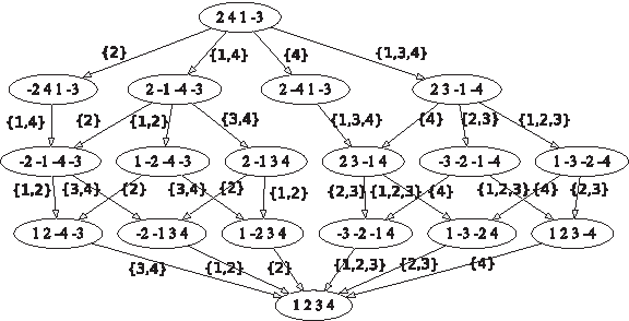
Siepel (2002) was the first to enumerate all sorting solutions as sequences of sorting reversals. His algorithm (SE) design is basically the ASSR described in Section 3, where solutions are represented as sequences. According to the ASSR, the number of i-sequences at the i-level will be at most \documentclass{aastex}\usepackage{amsbsy}\usepackage{amsfonts}\usepackage{amssymb}\usepackage{bm}\usepackage{mathrsfs}\usepackage{pifont}\usepackage{stmaryrd}\usepackage{textcomp}\usepackage{portland, xspace}\usepackage{amsmath, amsxtra}\pagestyle{empty}\DeclareMathSizes{10}{9}{7}{6}\begin{document} $$n^2 * n^2 * \cdots * n^2$$ \end{document} (i times). This implies that at any i-level there are at most n²ⁱ i-sequences. Thus, the SE algorithm has to repeat the two steps in ASSR O(n²ⁱ) times for each i-level. Adding up the time complexity for all levels, SE lists all sorting sequences in O(n²ⁿ⁺³) time (Braga et al., 2008). For example in Figure 1, the permutation π = (2, 4, 1, −3) has 16 optimal sequences that are represented by all possible 16 paths in the graph.

FIG. 1.

The permutation π =(2, 4, 1, −3) has 16 optimal sorting sequences, represented by all possible 16 paths in the graph.

The algorithm is only feasible for small distances due to the huge number of sequences generated. For example, for the permutation (−10, 9, −8, 5, 11, −4, 2, 6, −7, 3, 1), the number of solutions is 8278540.

4.2. Generating solutions using normal forms of traces

Since the number of sorting sequences is huge, Bergeron et al. (2002) proposed that, for a given signed permutation π, the set of all sorting sequences can be classified into equivalence classes. They adapted the concept of traces to sorting sequences. However, the authors did not provide an algorithm to enumerate the classes without enumerating all the sequences.

Two reversals are said to overlap if they intersect but neither is contained in the other. For example, in the permutation π = (2, 4, 1, −3), the reversals {2,4} and {1,3,4} overlap, while {2,4} and {1,2,4} do not. If we identify a sequence of reversals with a word on the alphabet of reversals, an equivalence relation on these words can be established and forms classes, or “traces,” of solutions. A trace is an equivalence class of sorting sequences of reversals, where the equivalence relation is defined as follows: if ρ and θ are reversals and do not overlap, then the words ρθ and θρ are equivalent. We say that ρ and θ commute. Under this relation, two sorting sequences are said to be equivalent if one can be obtained from the other by a sequence of commutations of non-overlapping reversals.

For the permutation π = (2, 4, 1, −3), consider the solution given by the sequence of reversals {1,3,4}{4}{1,2,3}{2,3}. Here, {1,3,4} and {4} commute, so {1,3,4}{4}{1,2,3}{2,3} and {4}{1,3,4}{1,2,3}{2,3} are equivalent. These two permutations, along with 6 others, form a trace. The concept of traces is well studied in combinatorics (Diekert and Rozenberg, 1995). The number of subwords in a trace is its height, and the number of solutions a trace represents is its size.

A theorem by Cartier and Foata (1969) states that, for any trace, there is a unique word that is in normal form.

Definition 1 (normal form)

A trace T is in normal form if it can be decomposed into subwords \documentclass{aastex}\usepackage{amsbsy}\usepackage{amsfonts}\usepackage{amssymb}\usepackage{bm}\usepackage{mathrsfs}\usepackage{pifont}\usepackage{stmaryrd}\usepackage{textcomp}\usepackage{portland, xspace}\usepackage{amsmath, amsxtra}\pagestyle{empty}\DeclareMathSizes{10}{9}{7}{6}\begin{document} $$s = u_1 | \ldots | u_m$$ \end{document} such that:

• every pair of elements of a subword u_i commute;

• for every element ρ of a subword u_i(i > 1), there is at least one element θ of the subword u_i–1 such that ρ and θ do not commute;

• every subword u_i is a nonempty increasing word under the lexicographic order.

For example, in Figure 2, the permutation π = (2, 4, 1, −3) has two normal forms representing sorting sequences: {1,3,4}{4} | {1,2,3}{2,3} (red paths) and {1,4}{2} | {1,2}{3,4} (black paths). The two normal forms of the traces describes the entire set of 16 sequences in a compact way.

FIG. 2.

The permutation π = (2, 4, 1, −3) has two normal forms representing sorting sequences: {1,3,4}{4} | {1,2,3}{2,3} (red paths) and {1,4}{2} | {1,2}{3,4} (black paths).

Braga et al. (2008) and Braga (2009) developed an algorithm (BR) to generate normal forms of traces. BR is also basically the ASSR as described in Section 2, where solutions are represented as normal forms of traces, NFtraces. Their idea was based on the fact that each (i − 1)-NFtrace is a prefix for an i-NFtrace.

Again, as in the ASSR, for each i-NFtrace, BR (Braga, 2009) applies Siepel's ASR algorithm to generate the next sorting reversals. These sorting reversals are then inserted into the normal form in the appropriate position to build a normal form of length i + 1. The costly operation here is inserting the new normal form into the exponentially large set of (i + 1)-NFtraces. The BR algorithm lists all sorting solutions as d(π)-NFtraces. Since we can count the number of times a particular normal form is inserted into the set of (i + 1)-NFtraces, we can count the number of sorting sequences leading to any normal form.

It was shown empirically that the BR algorithm had a great impact on the speed of enumerating traces. The savings come from the fact that the number of i-NFtraces at each i-level in BR is much smaller than the number of i-sequences at the same i-level in SE. Accordingly, the number of times the two steps in ASSR are repeated is much smaller in BR than that in SE. The complexity of BR depends on the total number of i-NFtraces at each i-level. Since each i-NFtrace is a prefix of a d-NFtrace, this number is bounded by the number of d-NFtraces times the number of prefixes of each i-NFtrace. The complete analysis was done in Braga et al. (2008), where the i-NFtraces were represented as posets, and where it was proved that the complexity of BR is bounded by O(Nn^kmax+4), where N is the number of d-NFtraces and k_max is the maximum width of any normal form as defined in Braga et al. (2008).

BR is a general algorithm in that many constraints can be applied to the sorting sequences it considers (Braga et al., 2009). Unfortunately, the BR algorithm needs a potentially exponential amount of memory or extensive disk use, making it feasible only for distances up to 13 (Braga, 2009).

4.3. Generating solutions using normal forms of traces with appended sorting reversals

More recent work by Baudet and Dias (2010) generates normal forms of traces in a more precise way. As with BR, their algorithm (BD) follows the ASSR representing i-solutions as i-NFtraces. To improve memory usage, they made use of the fact that not all sorting reversals calculated by Siepel's ASR algorithm are needed for every i-NFtrace.

Let an appended sorting reversal to a NFtrace be a sorting reversal that, when added to the normal form, will be the last reversal in the NFtrace. For example, for π = (2, 4, 1, −3) with NFtraces {1,3,4}{4} | {1,2,3}{2,3} and {1,4}{2} | {1,2}{3,4}. The set of 1-NFtraces is {{1,3,4},{4},{1,4},{2}}. For the 1-NFtrace {1,3,4} the sorting reversal {4} is an appended sorting reversal, while for the 1-NFtrace {4} the sorting reversal {1,3,4} is a non-appended sorting reversal. Figure 3 shows the resultant graph, where red branches represent those paths that will not be explored because corresponding reversals are not appended sorting reversals.

FIG. 3.

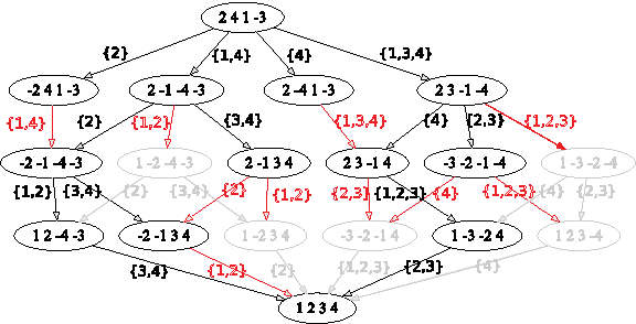
Sorting paths for the permutation π = (2, 4, 1, −3), where red branches represent those paths that will not be explored because corresponding reversals are not appending sorting reversals

Baudet and Dias (2010) changed BR in two ways. First, they add a sorting reversal to an i-NFtrace only if that reversal is an appended sorting reversal. Second, they generated i-NFtraces in a depth-first manner. As a result of the first improvement, every (i + 1)-NFtrace added to the (i + 1)-level will be unique; each (i + 1)-NFtrace can be visited in exactly one way by appended reversals. This decreases the time needed since there is no longer a search for duplicate (i + 1)-NFtraces in the (i + 1)-level. As a result of the second improvement, the algorithm requires only O(n³) space, whereas BR keeps all i-NFtraces. They used a stack of stacks to process these prefixes in a depth-first manner.

We now examine the connection between BR and BD in more detail.

Remark 1

The number of i-NFtraces, 1 ≤ i ≤ d, that BR and BD visit are the same.

This can be seen by again noting that for every i-NFtrace, there is exactly one series of appended sorting reversals that will create it. Remark 1 highlights the fact that Siepel's ASR algorithm is called the same number of times by BR and BD so that the only difference is that BD will generate a given i-NFtrace exactly once, whereas BD could generate the same i-NFtrace an exponential (in the size of the permutation) number of times.

BD also lends itself to a simple worst-case analysis. This is the first analysis for the problem of ASSR to give a bound on the time required to list each trace.

Theorem 1

For a permutation of length n at distance d from the identity, the time that it takes BD to list a normal form is O(n⁴2ⁿ).

Proof

Call an i-NFtrace that has no appended sorting reversals (in the set computed by Siepel's ASR algorithm) a dead-end. We show that for each d – NFtrace BD finds, there are O(2ⁿ) dead-ends. Assume a d – NFtrace T has only one subword (i.e., all sorting reversals commute), then for every subset of i (1 ≤ i ≤ d) reversals from T, there exists a dead-end I – NFtrace. So the number of dead-ends corresponding to T is the same as the number of substrings of a string, 2^d. Now take a d – NFtrace S with more than one subword. The number of substrings corresponding to S is fewer than the number of substrings corresponding to T since the existence of more than one subword indicates that at least two reversals do not commute. This, along with the fact that each dead-end visited costs O(n⁴), gives us the desired bound. ▪

An issue with the BD algorithm is that it cannot count the total number of sorting sequences corresponding to the generated normal forms (counting the number of linear extensions on a poset is #P-complete [Brightwell and Winkler, 1991]). Also, it cannot work when certain constraints are put on the sorting sequences; since it directly enumerates the normal forms of the traces, it cannot find traces that have compliant sorting sequences when the normal form itself does not comply with a particular constraint.

5. Permutation Grouping: An Improved Framework for ASSR

In the ASSR described in Section 3, Siepel's ASR algorithm is called for every i-solution at each i-level. In this section, we propose a new framework for the ASSR problem (ASSR-PG), where i-solutions are grouped at each i-level according to the corresponding permutations that they generate. The proposed ASSR-PG ensures that the ASR algorithm is called exactly once for each permutation that is generated throughout the course of the algorithm. The theorem below motivates this new approach.

Lemma 1

Consider the permutations along a sorting sequence \documentclass{aastex}\usepackage{amsbsy}\usepackage{amsfonts}\usepackage{amssymb}\usepackage{bm}\usepackage{mathrsfs}\usepackage{pifont}\usepackage{stmaryrd}\usepackage{textcomp}\usepackage{portland, xspace}\usepackage{amsmath, amsxtra}\pagestyle{empty}\DeclareMathSizes{10}{9}{7}{6}\begin{document} $$\pi_0 , \pi_1 , \ldots , \pi_d$$ \end{document} from π₀ to π_d. The number of i-NFtraces that when applied to π₀ yields π_i is monotonically increasing with i.

Proof

Call T the set of i-NFtraces that yield π_i when applied to π₀. There is exactly one reversal ρ such that \documentclass{aastex}\usepackage{amsbsy}\usepackage{amsfonts}\usepackage{amssymb}\usepackage{bm}\usepackage{mathrsfs}\usepackage{pifont}\usepackage{stmaryrd}\usepackage{textcomp}\usepackage{portland, xspace}\usepackage{amsmath, amsxtra}\pagestyle{empty}\DeclareMathSizes{10}{9}{7}{6}\begin{document} $$\pi_i \circ \rho = \pi_i{_+}_1$$ \end{document} . By inserting ρ into each of the normal forms for T, we get a unique (i + 1)-NFtrace because each pair of normal forms in T differ by at least one reversal, and we add the same element to all of them. ▪

Theorem 2

The ratio of the number of i-NFtraces to the number of permutations at an i-level is monotonically increasing with i.

Proof

The proof follows directly from Lemma 1. ▪

Figure 4 shows the average ratio (over 20 runs) of the number of normal forms of traces to the number of permutations for 7 ≤ n ≤ 14.

FIG. 4.
The average ratio between the number of normal forms of traces to the number of permutations visited during a run of BR, for permutations chosen uniformly at random.

5.1. The ASSR-PG

Let us first define the following notation:
• i-plevel: all permutations that are generated at distance d(π) – i by any i-solution.

• i-p: a permutation in the i-plevel.

• i-S: the set of optimal sorting reversals obtained by applying Siepel's ASR algorithm to an i-p.

• i-pgroup: a group of i-solutions, where each i-solution in that group generates the same permutation i-p. Each i-p has one group.

The new framework, ASSR-PG, can be modeled as follows:

For each i-p with corresponding i-pgroup, generate a set of (i+1)-solutions in the following two steps:
• Step 1: generate i-S for the i-p.

• Step 2: for each reversal ρ in i-S:

—insert ρ in each i-solution in its corresponding i-pgroup to generate a set of (i + 1)- solutions.

—generate \documentclass{aastex}\usepackage{amsbsy}\usepackage{amsfonts}\usepackage{amssymb}\usepackage{bm}\usepackage{mathrsfs}\usepackage{pifont}\usepackage{stmaryrd}\usepackage{textcomp}\usepackage{portland, xspace}\usepackage{amsmath, amsxtra}\pagestyle{empty}\DeclareMathSizes{10}{9}{7}{6}\begin{document} $(i + 1)\hbox{-p} = i \hbox{-}\rho \circ \rho$ \end{document} . Then we have the following two cases:

Case 1 (i + 1)-p is a new permutation: create a new group (i + 1)-pgroup using the generated set of (i + 1)-solutions.

Case 2 (i + 1)-p has already been generated: append the generated set of (i + 1)-solutions to the corresponding (i + 1)-pgroup.

These two steps are repeated iteratively until all optimal sorting d(π)-solutions are in the d(π)-pgroup and the d(π)-plevel will have only the identity permutation.

5.2. ASSR-PG algorithms

In order to process permutations, we use a hash table to store the permutation groups that can be generated at each i-plevel. The key for the hash table is the permutation i-p, and the data is the corresponding i-pgroup. This will help to test whether a given permutation has already been generated and to easily add solutions to their corresponding groups. Variations of the ASSR-PG approaches will again depend on how sorting solutions are represented. We have the following algorithms:
• Solutions are represented as sorting sequences (SE-PG). The SE algorithm (Siepel, 2002) can be updated so it conforms to the proposed framework, where solutions are represented as sequences. Additional savings will come from the fact that the ASR algorithm will be applied once per permutation rather than once per i-sequence generated.

• Solutions are represented as normal forms of traces, where normal forms are generated using all sorting reversals (BR-PG). Again, the BR algorithm (Braga, 2009) can be easily updated so that it conforms to the proposed framework, where solutions are represented as normal forms of traces. When using normal forms of traces, Braga et al. has to sort each i-pgroup to remove any repetitions. Since the number of NFtraces per group in BR-PG is much smaller than the number of NFtraces per level in BR, savings will be also achieved in sorting the NFtraces per group versus per level. Savings will come from the fact that Siepel's ASR algorithm will be applied once per permutation rather than once per i-NFtrace.

• Solutions are represented as normal forms of traces, where normal forms are generated with appended sorting reversals (BD-PG). The BD algorithm (Baudet and Dias, 2010) is the best known algorithm for solving the ASSR problem. However, the BD algorithm still calls the ASR algorithm more than once per permutation generated during the sorting process. We can update BD to optimize these calls and at the same time represent solutions as normal forms of traces that have been generated by appended sorting reversals as described in Section 4.3. However, the BD-PG algorithm will process the normal forms of traces in a breadth-first manner, grouping together those that generate the same permutation at each level.

To analyze the time complexity of these algorithms with high precision, the ratio of the number of solutions to the number of permutations at each level would have to be known. This will vary depending on the permutation so an average-case analysis may be the best we can hope for. We do not attempt such an analysis here. However, empirical results will be provided in Section 6 showing the savings that can be obtained when applying the new ASSR-PG for each of the three approaches.

6. Empirical Results

Extensive experiments were done to compare the original ASSR to the enhanced ASSR-PG. Starting from the original Java source code for Braga (2009) (baobabLUNA), we implemented the new techniques with the same Java objects. All the tests were performed using a single core of a 2.2-GHz Quad-Core AMD Opteron^(tm) Processor 8354 with 512 KB of cache and 132 G of memory.

We used the same experimental setup as Baudet and Dias (2010). We generated random permutations with size range between 5 ≤ n ≤ 26. For each value of n, we considered permutations with reversal distances d₁ = ⌈(n + l)/2⌉, d₂ = ⌈3n/4⌉, and d₃ = n. Since hurdles have a small probability of occurrence in random permutations, Swenson et al. (2008), Braga et al., and Baudet et al. considered only the permutations that have no hurdles. We did the same.

To show the advantages of the proposed ASSR-PG, for each set of permutations with parameters (n, d), we compared each approach when the original ASSR is applied to the same approach when the ASSP-PG is applied. In other words, we conduct three sets of experiments, where set 1 compares SE with SE-PG, set 2 compares BR with BR-PG, and set 3 compares BD with BD-PG.

The proposed ASSR-PG shows time improvements for all three base methods. Figure 5 shows the results comparing BR and BR-PG. Note the logarithmic scale. Improvements in time performance is up to 70%. Figure 6 shows time performance in seconds comparing BD and BD-PG, where applying the new framework decreases BD time by up to 50%. The results show that BR-PG cannot beat BD or BD-PG. The number of paths explored in the latter algorithms is much smaller, because only normal forms with reversals added at the end are explored. Results for comparing SE and SE-PG are not shown, but our experiments show that applying the new ASSR-PG greatly decreases the time required by SE.

FIG. 5.
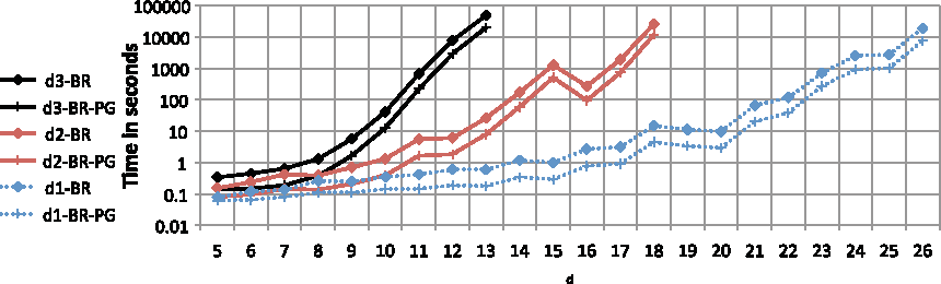
The time in seconds comparing BR and BR-PG, where d₁ = ⌈(n + l)/2⌉, d₂ = ⌈3n/4⌉, and d₃ = n.

FIG. 6.
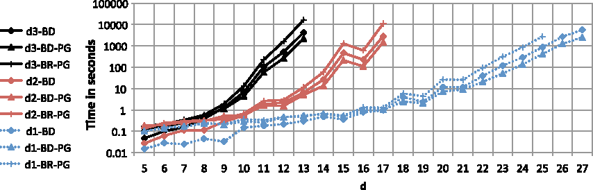
The time in seconds comparing BR-PG, BD, and BD-PG, where d₁ = ⌈(n + 1)/2⌉, d₂ = ⌈3n/4⌉, and d₃ = n.

7. Conclusion

We revisited the problem of finding ASSR. We showed that all approaches for solving the problem can be situated in the same fundamental framework, the ASSR. This allowed us to compare all current approaches. We also proposed an enhanced framework, the ASSR-PG, for solving the same problem by grouping partial solutions according to the corresponding permutations that they generate. The ASSR-PG ensures that the ASR algorithm is called exactly once for each permutation that is generated throughout the course of the algorithms. Extensive experiments were done that empirically demonstrate the speed-up that can be achieved by applying the ASSR-PG. The results showed that, by applying the new framework, we achieved an algorithm that beats the fastest known algorithm to solve the ASSR problem.

Footnotes

Acknowledgments

We would like to thank M.D.V. Braga for providing the Java source for the baobab-LUNA software (Braga, ). Research was partially funded by an NSERC Discovery Grant to DS.

Disclosure Statement

No competing financial interests exist.

1

The framework we present in Section 5 also uses this algorithm. Our recent result, Swenson et al. (), shows that ASR can be solved in O(n²) time on average, which would introduce a significant speed-up on all known algorithms for the ASSR problem. In this article, we focus on the improvement gained through our new framework although using the two together is sure to provide even stronger results.

References

Ajana

, Lefebvre

J.-F.

, Tillier

E.R.M.

et al. 2002. Exploring the set of all minimal sequences of reversals—an application to test the replication-directed reversal hypothesis. Proc. WABI'02, 300–315.

Baudet

, Dias

2010. An improved algorithm to enumerate all traces that sort a signed permutation by reversals. Proc. 2010 ACM Symp. Appl. Comput., 1521–1525.

Bergeron

, Chauve

, Hartman

et al. 2002. On the properties of sequences of reversals that sort a signed permutation. Proc. JOBIM, 99–108.

Braga

M.D.V.

2009. BaobabLUNA: the solution space of sorting by reversals. Bioinformatics, 25:1833–1835.

Braga

M.D.V.

, Sagot

M.-F.

, Scornavacca

et al. 2008. Exploring the solution space of sorting by reversals, with experiments and an application to evolution. IEEE/ACM Trans. Comput. Biol. and Bioinform., 5:348–356.

Braga

M.D.V.

, Gautier

, Sagot

2009. An asymmetric approach to preserve common intervals while sorting by reversals. Algorithms Mol. Biol., 4:16.

Caprara

1997. Sorting by reversals is difficult. Proc. RECOMB'97, 75–83.

Cartier

, Foata

1969. Problèmes combinatoires de commutations set réarrangements. Lect. Notes Math, 85.

Diekert

, Rozenberg

1995. The Book of Traces. World Scientific: New York.

10.

Brightwell

, Winkler

1991. Counting linear extensions is #p-complete. Proc. 23rd Annu. ACM Symp. Theory Comput., 175–181.

11.

Hannenhalli

, Pevzner

P.A.

1995. Transforming cabbage into turnip (polynomial algorithm for sorting signed permutations by reversals) Proc. 27th Annu. ACM Symp. Theory of Comput. (STOC'95), 178–189.

12.

Siepel

A.C.

2002. An algorithm to find all sorting reversals. Proc. 6th Annu. Int. Conf. Comput. Mol. Biol. (RECOMB'02), 281–290.

13.

Swenson

K.M.

, Rajan

, Lin

et al. 2009. Sorting signed permutations by inversions in o(nlogn) time. Lect. Notes Comput. Sci., 5541:386–399.

14.

Swenson

K.M.

, Lin

, Rajan

et al. 2008. Hurdles hardly have to be heeded. Lect. Notes Comput. Sci., 5267:239–249.

15.

Swenson

K.M.

, Badr

, Sankoff

2010. Listing all sorting reversals in quadratic time. Lect. Notes Comput. Sci., 102–110.

16.

Tannier

, Bergeron

, Sagot

M.F.

2007. Advances on sorting by reversals. Disc. Appl Math., 155:881–888.