Using Noise for Model-Testing

Abstract

For realistic models in molecular biology, you need to consider the noise in the cellular and intracellular environments. In this article, we present a novel approach for testing the validity of nonlinear models representing a biological system affected by noise. Our approach is based on results by Kushner and Øksendal and uses computational techniques that rely on efficient solvers. By providing analytically upper bounds for the exit probability of solution trajectories of a system from a particular set in the phase space, we can compare measurement data with this prediction and try to invalidate models with certain parameter values or noise properties. Thus, our approach complements the usual methods that are based on deterministic models. It is particularly useful in the field of reverse engineering in systems biology, when one seeks to determine model parameters and noise properties as we show in the Results section, where we applied the approach to examples of increasing complexity and to the Hog1 signalling pathway.

1. Introduction

In order to reduce modeling and analysis complexity, one often represents biological systems using deterministic models. This is a good approximation for the behavior in the continuous-flow, well-stirred tank reactor (CSTR) of the chemical industry or for systems investigated in vitro. However, for systems with few reactants, such as the cell, one needs to consider stochasticity to obtain a true picture of the dynamics (El-Samad et al., 2006a,b; Munsky et al., 2009). For instance, there is an inherent stochasticity in biochemical processes, which is called intrinsic noise (El-Samad and Khammash, 2004). Fluctuations in the amounts of chemicals or their concentrations due to the environment or changes in the environment is called extrinsic noise (Elowitz et al., 2002; Shahrezaei et al., 2008; Sotiropoulos et al., 2009; Komorowski et al., 2010).

There are various reasons for the different types of noise in vivo. Many vital reactions happen between extracellular ligands, such as signal molecules, hormones, and receptors on the membrane of the cell, and between intracellular molecules and receptors on the membrane of organelles within the cell. Additionally, nutrients have to enter the cell by passing through the membrane and then interact with structural proteins and lipids. In other words, the mixing of molecules often can be obstructed.

Moreover, molecular reactions greatly depend on the availability of reaction volume. If a molecule, which participates in the reaction, is much smaller than the background molecules, then they have no, or only weak, influence on the reaction rate as the molecule can freely diffuse between them. On the other hand, the diffusion of molecules of similar size would be greatly hindered. This effect is called the volume exclusion effect (Schnell and Turner, 2004). In other words, a small molecule can easily occupy the volume in between obstacles, while the volume a molecule can occupy, whose size is of order of the obstacles, is greatly limited.

The success of systems biology depends on the ability to use computational models to unravel underlying biological mechanisms. These models often correspond to biological hypotheses, for example, about the underlying reaction network structure or the type and strength of noise. It is well known, however, that models of comparable complexity corresponding to different pathway connectivities may fit experimental data equally well (Roberts et al., 2009). Model-testing approaches that invalidate models can be used to reduce the number of possible models.

One shortcoming of current experimental design approaches for discriminating between rival mathematical models representing a biological system is that they often use a linearized version of models or cannot deal well with experimental noise and parameter uncertainties (August and Busch, 2011). Despite the fact that the cellular and intracellular environments are noisy, in silico model analysis for model-testing is mostly based on underlying models that are deterministic (see Mélykúti et al., 2010, and references therein). For these reasons, in this article we develop a novel model-testing approach based on “listening to the noise” (Munsky et al., 2009). We use the results of Øksendal (2003) and Kushner (1967) to present a state-of-the-art system analysis framework.

The structure of this article is as follows: In Section 2, we present different approaches to modeling and model-testing. We also show how the tests can be implemented computationally using new, state-of-the-art tools. For clarity, we describe these tools first, in Section 2.1. In Section 2.2, we briefly describe the deterministic modeling approach to biological systems, which is typically used in chemical reaction network theory (Feinberg, 1987), and a computational approach to test its stability.

However, because assuming deterministic dynamics is not always suitable for analyzing biological systems as argued previously, in Section 2.3 we introduce the notion of stochastic differential equations used for mathematical modeling of noisy systems. We present established results on estimating the exit probability of the solution trajectory of a system from a particular set in the phase space. We then provide a novel algorithm for model-testing using these results. Section 3 provides examples validating our approach to model-testing and its application to the Hog1 signaling pathway, allowing for the analysis of noise. We conclude the article in Section 4.

2. Methods

2.1. Semidefinite programming and the sum of squares decomposition

In this section, we provide some mathematical background on the computational tools we use for model-testing. These tools can also be used to computationally implement and solve other problems that arise in the field of model-analysis in biology (El-Samad et al., 2006b; August and Papachristodoulou, 2009). The main computational tool is semidefinite programming (Vandenberghe and Boyd, 1996), which can be solved efficiently using interior-point methods (Boyd and Vandenberghe, 2004). In semidefinite programming, we replace the nonnegative orthant constraint of linear programming by the cone of positive semidefinite matrices and pose the following minimization problem: \documentclass{aastex}\usepackage{amsbsy}\usepackage{amsfonts}\usepackage{amssymb}\usepackage{bm}\usepackage{mathrsfs}\usepackage{pifont}\usepackage{stmaryrd}\usepackage{textcomp}\usepackage{portland,xspace}\usepackage{amsmath,amsxtra}\pagestyle{empty}\DeclareMathSizes{10}{9}{7}{6} \begin{document} \begin{align*} {\rm minimize} \quad & {\bf c}^{\rm T}{\bf x} \\ {\rm subject \ to} \quad & {\bf M} ({\bf x}) \geq 0, {\rm where \ {\bf M}} ({\bf x}) = {\bf M}_0 + \sum_{i = 1}^n {\bf x}_i{\bf M}_i. \tag{1} \end{align*} \end{document}

Here, \documentclass{aastex}\usepackage{amsbsy}\usepackage{amsfonts}\usepackage{amssymb}\usepackage{bm}\usepackage{mathrsfs}\usepackage{pifont}\usepackage{stmaryrd}\usepackage{textcomp}\usepackage{portland, xspace}\usepackage{amsmath, amsxtra}\pagestyle{empty}\DeclareMathSizes {10} {9} {7} {6} \begin{document} $${\bf x} \in {\mathbb R}^n$$\end{document} is the free variable. The so-called problem data, which are given, are the vector \documentclass{aastex}\usepackage{amsbsy}\usepackage{amsfonts}\usepackage{amssymb}\usepackage{bm}\usepackage{mathrsfs}\usepackage{pifont}\usepackage{stmaryrd}\usepackage{textcomp}\usepackage{portland, xspace}\usepackage{amsmath, amsxtra}\pagestyle{empty}\DeclareMathSizes {10} {9} {7} {6} \begin{document} $${\bf c} \in {\mathbb R}^n$$\end{document} and the matrices \documentclass{aastex}\usepackage{amsbsy}\usepackage{amsfonts}\usepackage{amssymb}\usepackage{bm}\usepackage{mathrsfs}\usepackage{pifont}\usepackage{stmaryrd}\usepackage{textcomp}\usepackage{portland, xspace}\usepackage{amsmath, amsxtra}\pagestyle{empty}\DeclareMathSizes {10} {9} {7} {6} \begin{document} $${\bf M}_j \in {\mathbb R}^{m \times m}, j = 0, \ldots, n$$\end{document} . Note that convexity of the set of symmetric positive semidefinite matrices in Eq. (1) implies that the minimization problem has a global minimum.

2.1.1. Sum of squares decomposition

For problem data that consists of polynomials of any degree, the requirement of positivity can be relaxed to the condition that the polynomial function is a sum of squares (SOS). On one hand, this is only a sufficient condition for positivity and can at times be quite conservative; in other words, a function can be positive without being an SOS. On the other hand, testing positivity of a polynomial can be NP-hard (Murty and Kabadi, 1987).

Consider the real-valued polynomial function F(x) of degree 2d, \documentclass{aastex}\usepackage{amsbsy}\usepackage{amsfonts}\usepackage{amssymb}\usepackage{bm}\usepackage{mathrsfs}\usepackage{pifont}\usepackage{stmaryrd}\usepackage{textcomp}\usepackage{portland, xspace}\usepackage{amsmath, amsxtra}\pagestyle{empty}\DeclareMathSizes {10} {9} {7} {6} \begin{document} $${\bf x} \in {\mathbb R}^n$$\end{document} . A sufficient condition for F(x) to be nonnegative is that it can be decomposed into an SOS (Parrilo, 2003): \documentclass{aastex}\usepackage{amsbsy}\usepackage{amsfonts}\usepackage{amssymb}\usepackage{bm}\usepackage{mathrsfs}\usepackage{pifont}\usepackage{stmaryrd}\usepackage{textcomp}\usepackage{portland, xspace}\usepackage{amsmath, amsxtra}\pagestyle{empty}\DeclareMathSizes {10} {9} {7} {6} \begin{document} $$F ({\bf x}) = \sum_i g_i^2 ({\bf x}) \geq 0$$\end{document} , where g_i are polynomial functions. Now, F(x) is an SOS if and only if there exists a positive semidefinite matrix Q and \documentclass{aastex}\usepackage{amsbsy}\usepackage{amsfonts}\usepackage{amssymb}\usepackage{bm}\usepackage{mathrsfs}\usepackage{pifont}\usepackage{stmaryrd}\usepackage{textcomp}\usepackage{portland,xspace}\usepackage{amsmath,amsxtra}\pagestyle{empty}\DeclareMathSizes{10}{9}{7}{6} \begin{document} \begin{align*}F ({\bf x}) = {\bf z}^{\rm T} {\bf Q} {\bf z}, \quad {\bf z} = [ 1, \ x_1, \ x_2, \ldots, \ x_n, x_1x_2, \ldots, \ x^d_n].\end{align*}\end{document}

The length of vector z is \documentclass{aastex}\usepackage{amsbsy}\usepackage{amsfonts}\usepackage{amssymb}\usepackage{bm}\usepackage{mathrsfs}\usepackage{pifont}\usepackage{stmaryrd}\usepackage{textcomp}\usepackage{portland, xspace}\usepackage{amsmath, amsxtra}\pagestyle{empty}\DeclareMathSizes {10} {9} {7} {6} \begin{document} $$\ell = {n + d \choose d}$$\end{document} . Note that Q is not necessarily unique. However, \documentclass{aastex}\usepackage{amsbsy}\usepackage{amsfonts}\usepackage{amssymb}\usepackage{bm}\usepackage{mathrsfs}\usepackage{pifont}\usepackage{stmaryrd}\usepackage{textcomp}\usepackage{portland, xspace}\usepackage{amsmath, amsxtra}\pagestyle{empty}\DeclareMathSizes {10} {9} {7} {6} \begin{document} $$\sum_i g_i^2 ({\rm x}) = {\bf z}^{\rm T}{\bf Qz}$$\end{document} poses certain constraints on Q of the form trace(A_jQ) = c_j, where A_j and c_j are appropriate matrices and constants, respectively. (For an illustration, see Example 3.5 in Parrilo, 2003.) In general, to find Q we solve the optimization problem associated with the following semidefinite program: \documentclass{aastex}\usepackage{amsbsy}\usepackage{amsfonts}\usepackage{amssymb}\usepackage{bm}\usepackage{mathrsfs}\usepackage{pifont}\usepackage{stmaryrd}\usepackage{textcomp}\usepackage{portland,xspace}\usepackage{amsmath,amsxtra}\pagestyle{empty}\DeclareMathSizes{10}{9}{7}{6} \begin{document} \begin{align*}{\rm minimize} \ \quad & {\rm trace} ({\bf A}_0{\bf Q}) \\ {\rm subject} \ {\rm to} \ \quad & {\bf Q} \geq 0, \ {\rm and \ trace} ({\bf A}_j {\bf Q}) = c_j, \quad j = 1, \ldots , m. \tag{2} \end{align*}\end{document}

In this article, to solve SOS programs, we use SOSTOOLS (Prajna et al., 2002), a free, third-party MATLAB toolbox that relies on the solver SeDuMi (Sturm, 1999).

Note that the computational time necessary to solve sum of squares decomposition problems scales badly with the size of the problem (Table 1), which makes the application of our method to nonlinear models with more than five to six species prohibitive when using current solvers in MATLAB. Nonetheless, many models in biology do not consider more than six species.

Table 1.

Complexity of the Sum of Squares Decomposition

2d/n	1	3	5	7	9	11	13
2	2	4	6	8	10	12	14
4	3	10	21	36	55	78	105
6	4	20	56	120	220	364	560
8	5	35	126	330	715	1365	2380
10	6	56	252	792	2002	4368	8568
12	7	84	462	1716	5005	12376	27132

The dimension of matrix Q is a function of the number of variables n and the degree 2d of F(x) = z^TQz (Parrilo, 2003).

2.2. Deterministic modeling approach

Below, we briefly demonstrate the use of SOSTOOLS for checking system stability of a deterministic dynamical system used to represent a biological system. Consider the following set of ordinary differential equations representing a dynamical system with state vector x \documentclass{aastex}\usepackage{amsbsy}\usepackage{amsfonts}\usepackage{amssymb}\usepackage{bm}\usepackage{mathrsfs}\usepackage{pifont}\usepackage{stmaryrd}\usepackage{textcomp}\usepackage{portland,xspace}\usepackage{amsmath,amsxtra}\pagestyle{empty}\DeclareMathSizes{10}{9}{7}{6} \begin{document} \begin{align*}{\dot {\rm \bf x}} = {\bf b} ({\bf x}) , \quad {\bf x} \in {\mathbb R}^n , \tag{3}\end{align*}\end{document}

where function b : \documentclass{aastex}\usepackage{amsbsy}\usepackage{amsfonts}\usepackage{amssymb}\usepackage{bm}\usepackage{mathrsfs}\usepackage{pifont}\usepackage{stmaryrd}\usepackage{textcomp}\usepackage{portland, xspace}\usepackage{amsmath, amsxtra}\pagestyle{empty}\DeclareMathSizes {10} {9} {7} {6} \begin{document} $${\mathbb R}^n \rightarrow {\mathbb R}^n$$\end{document} describes the system's dynamics. If function b(x) is such that b(0) = 0 and b(x) is given by a polynomial function or a rational function consisting of polynomials then we can search for a Lyapunov function V(x) that proves stability of the origin by means of an SOS program. For instance, by successfully solving the following problem, we provide such a function. \documentclass{aastex}\usepackage{amsbsy}\usepackage{amsfonts}\usepackage{amssymb}\usepackage{bm}\usepackage{mathrsfs}\usepackage{pifont}\usepackage{stmaryrd}\usepackage{textcomp}\usepackage{portland,xspace}\usepackage{amsmath,amsxtra}\pagestyle{empty}\DeclareMathSizes{10}{9}{7}{6} \begin{document} \begin{align*} {\rm Given} \quad & \delta > 0 , \ {\bf b} ({\bf x}) , \ {\bf x} \in {\mathbb R}^n \\ {\rm find} \quad & V ({\bf x}) \\ {\rm subject} \ {\rm to} \quad & V ({\bf x}) \ {\rm is} \ {\rm SOS} - \frac{\partial V ({\bf x})^{\rm T}}{\partial {\bf x}} {\bf b} ({\bf x}) - \delta {\bf x}^{\rm T}{\bf x} \ {\rm is} \ {\rm SOS}.\tag{4} \end{align*}\end{document}

However, as mentioned in the introduction, for modeling certain biological systems, a stochastic approach is more realistic. In the following section, we introduce such an approach and provide novel means using SOSTOOLS to distinguish between different models affected by noise by comparing them with measurement data.

2.3. Stochastic modeling approach

Consider the following stochastic differential equation representing a dynamical system with random state vector X, \documentclass{aastex}\usepackage{amsbsy}\usepackage{amsfonts}\usepackage{amssymb}\usepackage{bm}\usepackage{mathrsfs}\usepackage{pifont}\usepackage{stmaryrd}\usepackage{textcomp}\usepackage{portland,xspace}\usepackage{amsmath,amsxtra}\pagestyle{empty}\DeclareMathSizes{10}{9}{7}{6} \begin{document} \begin{align*} {\rm d} {\bf X} = {\bf b} ({\bf X}) {\rm d}t + \epsilon {\bf \sigma} ({\bf X}) {\rm d}{\bf W} , \tag{5}\end{align*} \end{document}

where \documentclass{aastex}\usepackage{amsbsy}\usepackage{amsfonts}\usepackage{amssymb}\usepackage{bm}\usepackage{mathrsfs}\usepackage{pifont}\usepackage{stmaryrd}\usepackage{textcomp}\usepackage{portland, xspace}\usepackage{amsmath, amsxtra}\pagestyle{empty}\DeclareMathSizes {10} {9} {7} {6} \begin{document} $$\in$$\end{document} is a positive constant, W is a n-dimensional Wiener Process, b : \documentclass{aastex}\usepackage{amsbsy}\usepackage{amsfonts}\usepackage{amssymb}\usepackage{bm}\usepackage{mathrsfs}\usepackage{pifont}\usepackage{stmaryrd}\usepackage{textcomp}\usepackage{portland, xspace}\usepackage{amsmath, amsxtra}\pagestyle{empty}\DeclareMathSizes {10} {9} {7} {6} \begin{document} $${\mathbb R}^n \rightarrow {\mathbb R}^n$$\end{document} the drift function and \documentclass{aastex}\usepackage{amsbsy}\usepackage{amsfonts}\usepackage{amssymb}\usepackage{bm}\usepackage{mathrsfs}\usepackage{pifont}\usepackage{stmaryrd}\usepackage{textcomp}\usepackage{portland, xspace}\usepackage{amsmath, amsxtra}\pagestyle{empty}\DeclareMathSizes {10} {9} {7} {6} \begin{document} $${\bf \sigma}:{\mathbb R}^n \rightarrow {\mathbb R}^{n \times n}$$\end{document} the state-dependent diffusion matrix (Ventsel’ and Freidlin, 1970; Gihman and Skorohod, 1972).1 Both maps, b and σ, satisfy the usual conditions for the existence and uniqueness of solutions (El-Samad and Khammash, 2004). For the remainder of this article, we use the short-form notation σ for σ (X).

2.3.1. Exiting a set

For \documentclass{aastex}\usepackage{amsbsy}\usepackage{amsfonts}\usepackage{amssymb}\usepackage{bm}\usepackage{mathrsfs}\usepackage{pifont}\usepackage{stmaryrd}\usepackage{textcomp}\usepackage{portland, xspace}\usepackage{amsmath, amsxtra}\pagestyle{empty}\DeclareMathSizes {10} {9} {7} {6} \begin{document} $$\epsilon = 0$$\end{document} , let the origin be a stable equilibrium of Eq. (5). The infinitesimal generator for system (5) is given by A (Øksendal, 2003). For any given function \documentclass{aastex}\usepackage{amsbsy}\usepackage{amsfonts}\usepackage{amssymb}\usepackage{bm}\usepackage{mathrsfs}\usepackage{pifont}\usepackage{stmaryrd}\usepackage{textcomp}\usepackage{portland, xspace}\usepackage{amsmath, amsxtra}\pagestyle{empty}\DeclareMathSizes {10} {9} {7} {6} \begin{document} $$V ({\bf X}) \in C^{(2)}:{\mathbb R}^n \rightarrow {\mathbb R}$$\end{document} that is such that V(0) = 0 and V(X) > 0, otherwise if \documentclass{aastex}\usepackage{amsbsy}\usepackage{amsfonts}\usepackage{amssymb}\usepackage{bm}\usepackage{mathrsfs}\usepackage{pifont}\usepackage{stmaryrd}\usepackage{textcomp}\usepackage{portland,xspace}\usepackage{amsmath,amsxtra}\pagestyle{empty}\DeclareMathSizes{10}{9}{7}{6} \begin{document} \begin{align*} AV ({\bf X}) = \sum_i \left[b_i ({\bf X}) {\frac {\partial V ({\bf X})} {\partial X_ {i}}} + {\frac{\epsilon^2} {2}} \sum_j ({\bf \sigma} {\bf \sigma}^{\rm T}) _ {i , j} {\frac {\partial^2V ({\bf X})} {\partial X_iX_j}} \right] \leq0 \ \forall \textbf{X} \in {\cal A} \subset {\mathbb R}^n , \tag {6} \end{align*}\end{document}

then the expected value of V(X), given by E(V(X)), decreases with time or remains constant for all \documentclass{aastex}\usepackage{amsbsy}\usepackage{amsfonts}\usepackage{amssymb}\usepackage{bm}\usepackage{mathrsfs}\usepackage{pifont}\usepackage{stmaryrd}\usepackage{textcomp}\usepackage{portland, xspace}\usepackage{amsmath, amsxtra}\pagestyle{empty}\DeclareMathSizes {10} {9} {7} {6} \begin{document} $$\bf {X} \in {\cal A}$$\end{document} (Øksendal, 2003), where X evolves according to Eq. (5). Given a positive constant λ, Kushner (1967) shows that the following holds for any initial condition X(0) that is such that V(X(0)) < λ, \documentclass{aastex}\usepackage{amsbsy}\usepackage{amsfonts}\usepackage{amssymb}\usepackage{bm}\usepackage{mathrsfs}\usepackage{pifont}\usepackage{stmaryrd}\usepackage{textcomp}\usepackage{portland,xspace}\usepackage{amsmath,amsxtra}\pagestyle{empty}\DeclareMathSizes{10}{9}{7}{6} \begin{document} \begin{align*} P \left\{\sup_{0 < t < \infty} \ V ({\bf X}) \geq \lambda \ \bigg| \ {\bf X} (0) \right\} \leq {\frac {V ({\bf X} (0))} {\lambda}} , \tag {7} \end{align*}\end{document}

Let \documentclass{aastex}\usepackage{amsbsy}\usepackage{amsfonts}\usepackage{amssymb}\usepackage{bm}\usepackage{mathrsfs}\usepackage{pifont}\usepackage{stmaryrd}\usepackage{textcomp}\usepackage{portland, xspace}\usepackage{amsmath, amsxtra}\pagestyle{empty}\DeclareMathSizes {10} {9} {7} {6} \begin{document} $${\bf y} \in \partial G$$\end{document} . Then, for a given initial condition, function V evaluated on ∂G represents an upper bound on the set exit probability distribution. We denote by φ the value of function V, where V(y) is minimal on the boundary ∂G. In the next subsection, we use the following for model-testing: We compare the percentage of measured system trajectories that exit \documentclass{aastex}\usepackage{amsbsy}\usepackage{amsfonts}\usepackage{amssymb}\usepackage{bm}\usepackage{mathrsfs}\usepackage{pifont}\usepackage{stmaryrd}\usepackage{textcomp}\usepackage{portland, xspace}\usepackage{amsmath, amsxtra}\pagestyle{empty}\DeclareMathSizes {10} {9} {7} {6} \begin{document} $${\cal C}$$\end{document} through φ (that is, for which V(X) ≥ φ) with prediction (7). If the predicted upper bound of the probability to exit \documentclass{aastex}\usepackage{amsbsy}\usepackage{amsfonts}\usepackage{amssymb}\usepackage{bm}\usepackage{mathrsfs}\usepackage{pifont}\usepackage{stmaryrd}\usepackage{textcomp}\usepackage{portland, xspace}\usepackage{amsmath, amsxtra}\pagestyle{empty}\DeclareMathSizes {10} {9} {7} {6} \begin{document} $${\cal C}$$\end{document} through φ is lower than the measured one, then the model does not represent the data well.

2.3.2. Using set exit for model-testing

We consider a stopped process (Prajna et al., 2004) and a model of the form given by Eq. (5) for a system under observation. For initial condition X₀ and a given stopping criterion, let P_m be the measured percentage of trajectories for which f (X) ≥ λ, where f (X₀) < λ and \documentclass{aastex}\usepackage{amsbsy}\usepackage{amsfonts}\usepackage{amssymb}\usepackage{bm}\usepackage{mathrsfs}\usepackage{pifont}\usepackage{stmaryrd}\usepackage{textcomp}\usepackage{portland, xspace}\usepackage{amsmath, amsxtra}\pagestyle{empty}\DeclareMathSizes {10} {9} {7} {6} \begin{document} $$f ({\bf X}) \in C^{(2)}: {\mathbb R}^n \rightarrow {\mathbb R}$$\end{document} , f(X) > 0 if X ≠ 0 and f(0) = 0. Assuming ergodicity2, P_m equals the probability that f (X) ≥ λ given X₀. If V(X) = f (X) and the following holds for the model \documentclass{aastex}\usepackage{amsbsy}\usepackage{amsfonts}\usepackage{amssymb}\usepackage{bm}\usepackage{mathrsfs}\usepackage{pifont}\usepackage{stmaryrd}\usepackage{textcomp}\usepackage{portland,xspace}\usepackage{amsmath,amsxtra}\pagestyle{empty}\DeclareMathSizes{10}{9}{7}{6} \begin{document} \begin{align*} P \left\{\sup_ {0 < t < \infty} \ V ({\bf X}) \geq \lambda \ \bigg | \ {\bf X} _0 \right\} \leq {\frac {V ({\bf X} _0)} {\lambda}} < P_m , \tag{8} \end{align*}\end{document}

then the model predicts an upper bound on the probability that is lower than P_m, which is the measured one, and, thus, invalidates the model.

Generally, one must be very lucky if setting V(X) = f (X) yields inequality [Eq. (8)]. Indeed, Kushner (1967) mentions that the “Lyapunov function approach is often a crude approach. Given a tentative Lyapunov function, […] [if] there is to be no further analysis or search for other possible Lyapunov functions, then we must be content with the result given by a function which does not distinguish between quite different systems.” To answer Kushner's demand, the following result provides means to search for a different Lyapunov function in order to test the model.

Theorem 1.

Consider a model of the form given by Eq. (5) for a system under observation, an initial condition X₀. For a stopping criterion that halts the process, if ∥X∥ < γ,3 let P_m < 1 be the measured probability that ∥X∥ ≥ λ for initial condition X₀ such that ∥X₀∥ < λ. If the following problem has a solution then this solution invalidates the model. \documentclass{aastex}\usepackage{amsbsy}\usepackage{amsfonts}\usepackage{amssymb}\usepackage{bm}\usepackage{mathrsfs}\usepackage{pifont}\usepackage{stmaryrd}\usepackage{textcomp}\usepackage{portland,xspace}\usepackage{amsmath,amsxtra}\pagestyle{empty}\DeclareMathSizes{10}{9}{7}{6} \begin{document} \begin{align*} Given \quad & {\bf b} ({\bf X}) , \ \epsilon , \ {\bf \sigma} , \ {\bf X}_0 , \ f ({\bf X}) , \ \lambda , \ P_m , \ \delta > 0 \tag{9}\\ find \quad & V ({\bf X}) , \ \phi , \ p_i ({\bf X}) , \ i = 1 , \ldots , 4 \tag{10} \\ subject to \quad & V ({\bf X}) , \ \phi , \ p_i ({\bf X}) \ {\rm are \ SOS} , \ i = 1 , \ldots , 4 \tag{11}\\ & V ({\bf X}) - \phi + p_1 ({\bf X}) (\lambda - \ \mid{\bf X}\mid) \ {\rm is \ SOS} \tag{12} \\ & \phi P_m - V ({\bf X}) + p_3 ({\bf X}) \ \mid{\bf X} - {\bf X}_0\mid - \delta \ {\rm is \ SOS} \tag{13} \\ & - AV ({\bf X}) + p_4 ({\bf X}) (\gamma - \ \mid{\bf X}\mid) \ {\rm is \ SOS}. \tag{14} \end{align*} \end{document}

Proof.

Note that

Eq. (12) guarantees that if f (X) ≥ λ then V(X) ≥ φ.

Eq. (13) guarantees that if X = X₀ then V(X) < φP_m and, thus, that \documentclass{aastex}\usepackage{amsbsy}\usepackage{amsfonts}\usepackage{amssymb}\usepackage{bm}\usepackage{mathrsfs}\usepackage{pifont}\usepackage{stmaryrd}\usepackage{textcomp}\usepackage{portland, xspace}\usepackage{amsmath, amsxtra}\pagestyle{empty}\DeclareMathSizes {10} {9} {7} {6} \begin{document} $$ \frac {V ({\bf X} _0)} {\phi} < P_m$$\end{document} and moreover, that V(X₀) < φ, since P_m < 1.

Eq. (14) guarantees that if ∥X∥ ≥ γ then AV(X) ≤ 0.

Hence, if the problem given by Eqs (9)–(14) has a solution then \documentclass{aastex}\usepackage{amsbsy}\usepackage{amsfonts}\usepackage{amssymb}\usepackage{bm}\usepackage{mathrsfs}\usepackage{pifont}\usepackage{stmaryrd}\usepackage{textcomp}\usepackage{portland,xspace}\usepackage{amsmath,amsxtra}\pagestyle{empty}\DeclareMathSizes{10}{9}{7}{6} \begin{document} \begin{align*}P \left\{f ({\bf X}) \geq \lambda \ \bigg | \ {\bf X}_0 \right\} \ & \leq \ P \left\{V ({\bf X}) \geq \phi \ \bigg |\ {\bf X}_0 \right\} \\ & \leq \ P \left\{\sup_{0 < t < \infty} \ V ({\bf X}) \geq \phi \ \bigg | \ {\bf X}_0 \right\} < P_m, \end{align*}\end{document}

but since \documentclass{aastex}\usepackage{amsbsy}\usepackage{amsfonts}\usepackage{amssymb}\usepackage{bm}\usepackage{mathrsfs}\usepackage{pifont}\usepackage{stmaryrd}\usepackage{textcomp}\usepackage{portland,xspace}\usepackage{amsmath,amsxtra}\pagestyle{empty}\DeclareMathSizes{10}{9}{7}{6} \begin{document} \begin{align*}P \left\{ f ({\bf X}) \geq \lambda \ \bigg | \ {\bf X}_0 \right\} = P_m,\end{align*}\end{document}

this invalidates the model. ▪

3. Results

3.1. Two structurally different two-dimensional systems

3.1.1. Exit from a set

Consider the following van der Pol–like system presented in (Prajna et al., 2004): \documentclass{aastex}\usepackage{amsbsy}\usepackage{amsfonts}\usepackage{amssymb}\usepackage{bm}\usepackage{mathrsfs}\usepackage{pifont}\usepackage{stmaryrd}\usepackage{textcomp}\usepackage{portland,xspace}\usepackage{amsmath,amsxtra}\pagestyle{empty}\DeclareMathSizes{10}{9}{7}{6} \begin{document} \begin{align*} {\dot x} _1 \ & = \ x_2, \\ {\dot x} _2 \ & = \ - \left(x_1 + x_2 + \frac {1} {2} x_1^3 \right). \tag{15} \end{align*}\end{document}

The origin is the unique equilibrium point. The Lyapunov function given by \documentclass{aastex}\usepackage{amsbsy}\usepackage{amsfonts}\usepackage{amssymb}\usepackage{bm}\usepackage{mathrsfs}\usepackage{pifont}\usepackage{stmaryrd}\usepackage{textcomp}\usepackage{portland,xspace}\usepackage{amsmath,amsxtra}\pagestyle{empty}\DeclareMathSizes{10}{9}{7}{6} \begin{document} \begin{align*} \overline {V} ({\bf x}) = \frac {1} {2} \left(x_1^2 + x_2^2 + x_1x_2 \right) + \frac {1} {8} x_1^4 \tag {16} \end{align*}\end{document}

proves that the origin is globally asymptotically stable, since \documentclass{aastex}\usepackage{amsbsy}\usepackage{amsfonts}\usepackage{amssymb}\usepackage{bm}\usepackage{mathrsfs}\usepackage{pifont}\usepackage{stmaryrd}\usepackage{textcomp}\usepackage{portland,xspace}\usepackage{amsmath,amsxtra}\pagestyle{empty}\DeclareMathSizes{10}{9}{7}{6} \begin{document} \begin{align*} {\dot{\overline {V}}} ({\bf x}) = - \frac {1} {2} x_2^2 - \frac {1} {2} x_1 \left(x_1 + x_2 + \frac {1} {2} x_1^3 \right) < 0 , \quad {\bf x} \neq {\bf 0} .\end{align*}\end{document}

Set \documentclass{aastex}\usepackage{amsbsy}\usepackage{amsfonts}\usepackage{amssymb}\usepackage{bm}\usepackage{mathrsfs}\usepackage{pifont}\usepackage{stmaryrd}\usepackage{textcomp}\usepackage{portland, xspace}\usepackage{amsmath, amsxtra}\pagestyle{empty}\DeclareMathSizes {10} {9} {7} {6} \begin{document} $${\cal A}$$\end{document} is such that \documentclass{aastex}\usepackage{amsbsy}\usepackage{amsfonts}\usepackage{amssymb}\usepackage{bm}\usepackage{mathrsfs}\usepackage{pifont}\usepackage{stmaryrd}\usepackage{textcomp}\usepackage{portland,xspace}\usepackage{amsmath,amsxtra}\pagestyle{empty}\DeclareMathSizes{10}{9}{7}{6} \begin{document} \begin{align*} \overline {V} ({\bf X}) + \frac {1} {8} X_1^4 \geq0.245, \tag {18} \end{align*}\end{document}

since Eq. (6) holds if Eq. (18) holds. Let its boundary corresponds to the “inner” boundary of \documentclass{aastex}\usepackage{amsbsy}\usepackage{amsfonts}\usepackage{amssymb}\usepackage{bm}\usepackage{mathrsfs}\usepackage{pifont}\usepackage{stmaryrd}\usepackage{textcomp}\usepackage{portland, xspace}\usepackage{amsmath, amsxtra}\pagestyle{empty}\DeclareMathSizes {10} {9} {7} {6} \begin{document} $${\cal C}$$\end{document} . It is depicted by the inner ellipse in Figure 1. Let the “outer” boundary of \documentclass{aastex}\usepackage{amsbsy}\usepackage{amsfonts}\usepackage{amssymb}\usepackage{bm}\usepackage{mathrsfs}\usepackage{pifont}\usepackage{stmaryrd}\usepackage{textcomp}\usepackage{portland, xspace}\usepackage{amsmath, amsxtra}\pagestyle{empty}\DeclareMathSizes {10} {9} {7} {6} \begin{document} $${\cal C}$$\end{document} , which we denote by ∂G_o, be given by \documentclass{aastex}\usepackage{amsbsy}\usepackage{amsfonts}\usepackage{amssymb}\usepackage{bm}\usepackage{mathrsfs}\usepackage{pifont}\usepackage{stmaryrd}\usepackage{textcomp}\usepackage{portland, xspace}\usepackage{amsmath, amsxtra}\pagestyle{empty}\DeclareMathSizes {10} {9} {7} {6} \begin{document} $$\|{\bf X}\| _2^2 = 4$$\end{document} (black circle in Fig. 1). Then, for \documentclass{aastex}\usepackage{amsbsy}\usepackage{amsfonts}\usepackage{amssymb}\usepackage{bm}\usepackage{mathrsfs}\usepackage{pifont}\usepackage{stmaryrd}\usepackage{textcomp}\usepackage{portland, xspace}\usepackage{amsmath, amsxtra}\pagestyle{empty}\DeclareMathSizes {10} {9} {7} {6} \begin{document} $${\bf X} \in \partial G_o $$ \end{document} , the minimal value of \documentclass{aastex}\usepackage{amsbsy}\usepackage{amsfonts}\usepackage{amssymb}\usepackage{bm}\usepackage{mathrsfs}\usepackage{pifont}\usepackage{stmaryrd}\usepackage{textcomp}\usepackage{portland, xspace}\usepackage{amsmath, amsxtra}\pagestyle{empty}\DeclareMathSizes {10} {9} {7} {6} \begin{document} $${\overline V} ({\bf X})$$\end{document} evaluated on ∂G_o is obtained for X₁ = ±1.0305 and X₂ = ∓1.7141 and is given by φ = 1.2578. Note that for all initial conditions that are in set \documentclass{aastex}\usepackage{amsbsy}\usepackage{amsfonts}\usepackage{amssymb}\usepackage{bm}\usepackage{mathrsfs}\usepackage{pifont}\usepackage{stmaryrd}\usepackage{textcomp}\usepackage{portland, xspace}\usepackage{amsmath, amsxtra}\pagestyle{empty}\DeclareMathSizes {10} {9} {7} {6} \begin{document} $${\cal C}$$\end{document} , it follows from Eq. (7) that exit from the set by crossing ∂G_o is most probable at φ. For X₁(0) = −1.3 and X₂(0) = 1.3, it follows that \documentclass{aastex}\usepackage{amsbsy}\usepackage{amsfonts}\usepackage{amssymb}\usepackage{bm}\usepackage{mathrsfs}\usepackage{pifont}\usepackage{stmaryrd}\usepackage{textcomp}\usepackage{portland, xspace}\usepackage{amsmath, amsxtra}\pagestyle{empty}\DeclareMathSizes {10} {9} {7} {6} \begin{document} $$ \frac{{\overline V} ({\bf X}_0)} {\phi} = 0.9556 , {\bf X}_0 = {\bf X} (0)$$\end{document} . Figure 1 shows numerical realizations of Eq. (17). The dynamics of the process are shown in blue. The small red circles on ∂G_o correspond to X₁ = ±1.0305 and X₂ = ∓1.7141, where indeed exit from the set seems to occur quite often.

FIG. 1.

For X₁(0) = −1.3 and X₂(0) = 1.3, the figure shows numerical realizations of Eq. (17). The dynamics of the process are shown in blue. The outer black circle corresponds to \documentclass{aastex}\usepackage{amsbsy}\usepackage{amsfonts}\usepackage{amssymb}\usepackage{bm}\usepackage{mathrsfs}\usepackage{pifont}\usepackage{stmaryrd}\usepackage{textcomp}\usepackage{portland, xspace}\usepackage{amsmath, amsxtra}\pagestyle{empty}\DeclareMathSizes {10} {9} {7} {6} \begin{document} $$\|{\bf X}\|_2^2 = 4$$\end{document} , and the small red circles on it to X₁ = ±1.0305 and X₂ = ∓1.7141.

3.1.2. Model-Testing

Consider the van der Pol system: \documentclass{aastex}\usepackage{amsbsy}\usepackage{amsfonts}\usepackage{amssymb}\usepackage{bm}\usepackage{mathrsfs}\usepackage{pifont}\usepackage{stmaryrd}\usepackage{textcomp}\usepackage{portland,xspace}\usepackage{amsmath,amsxtra}\pagestyle{empty}\DeclareMathSizes{10}{9}{7}{6} \begin{document} \begin{align*} {\dot x} _1 \ & = \ x_2, \\ {\dot x} _2 \ & = \ - \left(x_1 + x_2 + \frac {1} {2} x_1^2x_2 \right). \tag{19} \end{align*}\end{document}

The origin is the only equilibrium point and globally asymptotically stable. This can be shown by means of the Lyapunov function given by \documentclass{aastex}\usepackage{amsbsy}\usepackage{amsfonts}\usepackage{amssymb}\usepackage{bm}\usepackage{mathrsfs}\usepackage{pifont}\usepackage{stmaryrd}\usepackage{textcomp}\usepackage{portland, xspace}\usepackage{amsmath, amsxtra}\pagestyle{empty}\DeclareMathSizes {10} {9} {7} {6} \begin{document} $$V ({\bf x}) = {\overline V} ({\bf x}) - \frac {1}{16} x_1^4$$\end{document} , where \documentclass{aastex}\usepackage{amsbsy}\usepackage{amsfonts}\usepackage{amssymb}\usepackage{bm}\usepackage{mathrsfs}\usepackage{pifont}\usepackage{stmaryrd}\usepackage{textcomp}\usepackage{portland, xspace}\usepackage{amsmath, amsxtra}\pagestyle{empty}\DeclareMathSizes {10} {9} {7} {6} \begin{document} $${\overline V} ({\bf X})$$\end{document} is given by Eq. (16). Let \documentclass{aastex}\usepackage{amsbsy}\usepackage{amsfonts}\usepackage{amssymb}\usepackage{bm}\usepackage{mathrsfs}\usepackage{pifont}\usepackage{stmaryrd}\usepackage{textcomp}\usepackage{portland, xspace}\usepackage{amsmath, amsxtra}\pagestyle{empty}\DeclareMathSizes {10} {9} {7} {6} \begin{document} $$\epsilon = 0.7 , \sigma_{11} = \sigma_{12} = \sigma_{21} = 0 , \ \sigma_{22} = 1$$\end{document} , and Eq. (19) be given in the form depicted in Eq. (5). Then \documentclass{aastex}\usepackage{amsbsy}\usepackage{amsfonts}\usepackage{amssymb}\usepackage{bm}\usepackage{mathrsfs}\usepackage{pifont}\usepackage{stmaryrd}\usepackage{textcomp}\usepackage{portland,xspace}\usepackage{amsmath,amsxtra}\pagestyle{empty}\DeclareMathSizes{10}{9}{7}{6} \begin{document} \begin{align*} {\rm d} X_1 \ & = \ X_2 \ {\rm d} t, \\ {\rm d} X_2 \ & = \ - \left(X_1 + X_2 + \frac {1} {2} X_1^2X_2 \right) \ {\rm d} t + 0.7 \ {\rm d} W. \tag{20} \end{align*}\end{document}

Assume that Eq. (17) is the system under investigation that we observe. For 20 times 100 realizations of Eq. (17) with X₁(0) = 2.8, X₂(0) = −2 and stopped if either \documentclass{aastex}\usepackage{amsbsy}\usepackage{amsfonts}\usepackage{amssymb}\usepackage{bm}\usepackage{mathrsfs}\usepackage{pifont}\usepackage{stmaryrd}\usepackage{textcomp}\usepackage{portland, xspace}\usepackage{amsmath, amsxtra}\pagestyle{empty}\DeclareMathSizes {10} {9} {7} {6} \begin{document} $$\|{\bf X}\|_2^2 < 5 \ {\rm or \ if} \ \|{\bf X}\|_2^2 \geq 9$$\end{document} , we observe that 81% of all runs, with a standard deviation of 5%, are terminated because of the latter. With b(X), \documentclass{aastex}\usepackage{amsbsy}\usepackage{amsfonts}\usepackage{amssymb}\usepackage{bm}\usepackage{mathrsfs}\usepackage{pifont}\usepackage{stmaryrd}\usepackage{textcomp}\usepackage{portland, xspace}\usepackage{amsmath, amsxtra}\pagestyle{empty}\DeclareMathSizes {10} {9} {7} {6} \begin{document} $$\epsilon $$\end{document} , and σ defined by Eq. (20), we solve the problem given by Eq. (9)–(14) using SOSTOOLS [a free third-party MATLAB toolbox (Prajna et al., 2002)] for P_m = 0.81, and obtain \documentclass{aastex}\usepackage{amsbsy}\usepackage{amsfonts}\usepackage{amssymb}\usepackage{bm}\usepackage{mathrsfs}\usepackage{pifont}\usepackage{stmaryrd}\usepackage{textcomp}\usepackage{portland,xspace}\usepackage{amsmath,amsxtra}\pagestyle{empty}\DeclareMathSizes{10}{9}{7}{6} \begin{document} \begin{align*} V ({\bf X}) = 0.151X_1^4 - 0.770X_1^3 + 0.128X_1^2X_2^2 + 1.298X_1^2 + 0.116X_1X_2^3 - 0.370X_1X_2^2 + 0.871{\bf x}_1X_2 + 0.154 {\bf x}_2^4 + 0.302X_2^3 + 1.594X_2^2\end{align*}\end{document}

and φ = 2.411. By Theorem 1, this implies that Eq. (20) can be invalidated as a model for system Eq. (17). Indeed, \documentclass{aastex}\usepackage{amsbsy}\usepackage{amsfonts}\usepackage{amssymb}\usepackage{bm}\usepackage{mathrsfs}\usepackage{pifont}\usepackage{stmaryrd}\usepackage{textcomp}\usepackage{portland,xspace}\usepackage{amsmath,amsxtra}\pagestyle{empty}\DeclareMathSizes{10}{9}{7}{6} \begin{document} \begin{align*} P \left\{\sup_{0 < t < \infty} \ V ({\bf X}) \geq \phi \ \bigg | \ {\bf X} _0 \right\} \leq {\frac {V ({\bf X} _0)} {\phi}} = 0.55 < P_m, \end{align*}\end{document}

where X₀ = X(0). An additional check for the validity of our computational model–invalidation approach is the fact that with b(X), \documentclass{aastex}\usepackage{amsbsy}\usepackage{amsfonts}\usepackage{amssymb}\usepackage{bm}\usepackage{mathrsfs}\usepackage{pifont}\usepackage{stmaryrd}\usepackage{textcomp}\usepackage{portland, xspace}\usepackage{amsmath, amsxtra}\pagestyle{empty}\DeclareMathSizes {10} {9} {7} {6} \begin{document} $$\epsilon$$\end{document} , and σ defined by Eq. (17), we indeed cannot solve the problem given by Eq. (9)–(14).

3.2. Parametrically different three-dimensional systems

Consider the lorenz-like system \documentclass{aastex}\usepackage{amsbsy}\usepackage{amsfonts}\usepackage{amssymb}\usepackage{bm}\usepackage{mathrsfs}\usepackage{pifont}\usepackage{stmaryrd}\usepackage{textcomp}\usepackage{portland,xspace}\usepackage{amsmath,amsxtra}\pagestyle{empty}\DeclareMathSizes{10}{9}{7}{6} \begin{document} \begin{align*} {\dot x}_1 \ & = \ x_2 - x_1, \\ {\dot x}_2 \ & = \ \frac {1}{2} x_1 - dx_2 - x_1x_3, \\ {\dot x}_3 \ & = \ x_1x_2 - 2x_3 - \frac {1} {4} x_1^2 , \tag{21} \end{align*}\end{document}

where d is a positive constant. The unique equilibrium point is the origin, whose stability can be shown via \documentclass{aastex}\usepackage{amsbsy}\usepackage{amsfonts}\usepackage{amssymb}\usepackage{bm}\usepackage{mathrsfs}\usepackage{pifont}\usepackage{stmaryrd}\usepackage{textcomp}\usepackage{portland,xspace}\usepackage{amsmath,amsxtra}\pagestyle{empty}\DeclareMathSizes{10}{9}{7}{6} \begin{document} \begin{align*}V ({\bf x}) = \frac {1} {2} \left(x_1^2 + x_2^2 + x_3^2 - \frac {1} {2} x_1x_2 \right) > 0 \ \forall {\bf x}, \ {\bf x} \neq {\bf 0}. \end{align*}\end{document}

Assume that, for d = 1, Eq. (22) is the system under investigation and the one that we observe. For 20 times 100 realizations of Eq. (22) with d = 1, X(0) = (1.1, −1.1, 0), and stopped if either \documentclass{aastex}\usepackage{amsbsy}\usepackage{amsfonts}\usepackage{amssymb}\usepackage{bm}\usepackage{mathrsfs}\usepackage{pifont}\usepackage{stmaryrd}\usepackage{textcomp}\usepackage{portland, xspace}\usepackage{amsmath, amsxtra}\pagestyle{empty}\DeclareMathSizes {10} {9} {7} {6} \begin{document} $$\|{\bf X}\|_2^2 < 2 \ {\rm or \ if} \ \|{\bf X}\|_2^2 \geq 3$$\end{document} , we observe that 27% of all runs, with a standard deviation of 6%, are terminated because of the latter. Let b(X), \documentclass{aastex}\usepackage{amsbsy}\usepackage{amsfonts}\usepackage{amssymb}\usepackage{bm}\usepackage{mathrsfs}\usepackage{pifont}\usepackage{stmaryrd}\usepackage{textcomp}\usepackage{portland, xspace}\usepackage{amsmath, amsxtra}\pagestyle{empty}\DeclareMathSizes {10} {9} {7} {6} \begin{document} $$\epsilon$$\end{document} and σ be defined by Eq. (22). For P_m = 0.27 and d = 5, we solve the problem given by Eq. (9)–(14) using SOSTOOLS and obtain \documentclass{aastex}\usepackage{amsbsy}\usepackage{amsfonts}\usepackage{amssymb}\usepackage{bm}\usepackage{mathrsfs}\usepackage{pifont}\usepackage{stmaryrd}\usepackage{textcomp}\usepackage{portland,xspace}\usepackage{amsmath,amsxtra}\pagestyle{empty}\DeclareMathSizes{10}{9}{7}{6} \begin{document} \begin{align*}V ({\bf X}) \ = \ & 7.74X_1^4 - 1.55X_1^3X_2 + 0.0001X_1^3X_3 - 16.2X_1^3 + 3.2X_1^2X_2^2 + 5.27X_1^2X_2 \\ & + 3.1 X_1^2X_3^2 - 24.3X_1^2X_3 + 8.65X_1^2 - 0.403X_1X_2^3 - 5.85X_1X_2^2 - 0.403X_1X_2X_3^2 \\ & + 12.3X_1X_2X_3 - 2.82X_1X_2 - 9.32X_1X_3^2 + 25.1X_1X_3 + 0.402X_2^4 + 1.86X_2^3 \\ & + 0.805X_2^2X_3^2 - 2.43X_2^2X_3 + 4.51X_2^2 - 3.26X_2 X_3^2 - 17.9X_2X_3 + 0.402X_3^4 \\ & + 2.89X_3^3 + 31.7X_3^2, \end{align*}\end{document}

and φ = 0.042. We conclude from Theorem 1 that this implies the model with d = 5 represents the data poorly.

3.3. Four-dimensional models for the Hog1 signaling pathway with different noise properties

The MAPK (mitogen activated protein kinase) Hog1 is the most downstream kinase of the signaling cascade, which is activated by osmotic stress (Hohmann et al., 2007). It is also a popular pathway in yeast for benchmark studies. The kinase activity of Hog1 in the cytoplasm leads to the production of glycerol (Westfall et al., 2008), which allows the cells to equilibrate interior and exterior osmotic pressures (Fig. 2). Importantly, this system is adaptive and concentrations of Hog1 quickly return to their preshock levels (Muzzey et al., 2009). This quickly adapting mechanism also allows for “kinetic specificity” such that the slower pheromone pathway is not activated after osmotic shock, albeit sharing some of the pathway components (Behar et al., 2007). 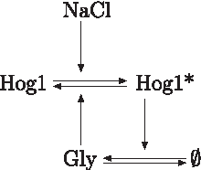The following adaptive model represents the described pathway: \documentclass{aastex}\usepackage{amsbsy}\usepackage{amsfonts}\usepackage{amssymb}\usepackage{bm}\usepackage{mathrsfs}\usepackage{pifont}\usepackage{stmaryrd}\usepackage{textcomp}\usepackage{portland,xspace}\usepackage{amsmath,amsxtra}\pagestyle{empty}\DeclareMathSizes{10}{9}{7}{6} \begin{document} \begin{align*} {\dot x}_1 \ & = \ - k_1x_1x_2 + k_3x_3 (C_2 - x_1 - (C_1 - x_2)), \\ {\dot x}_2 \ & = \ - k_1x_1x_2 + k_2 (C_1 - x_2), \\ {\dot x}_3 \ & = \ u (C_2 - x_1 - (C_1 - x_2)) - k_4x_3. \tag{23} \end{align*}\end{document}

FIG. 2.

A simple model for Hog1 activation.

Let k₁ = 1, k₂ = 0.1, k₃ = 2, k₄ = 3, C₁ = 5, C₂ = 6, and u = 4. Then, the positive equilibrium point of Eq. (2) is given by \documentclass{aastex}\usepackage{amsbsy}\usepackage{amsfonts}\usepackage{amssymb}\usepackage{bm}\usepackage{mathrsfs}\usepackage{pifont}\usepackage{stmaryrd}\usepackage{textcomp}\usepackage{portland,xspace}\usepackage{amsmath,amsxtra}\pagestyle{empty}\DeclareMathSizes{10}{9}{7}{6} \begin{document} \begin{align*}{\bf x}_{eq} = (1.029 , 0.443 , 0.551),\end{align*}\end{document}

and it is asymptotically stable. Here, x₁ denotes concentrations of inactive Hog1, x₂ of NaCl, x₃ of Glycerol, and C₁ the sum of the concentrations of Hog intermediates and NaCl; k₁ – k₄, u and C₂ are positive constants.

The following model assumes noisy total concentrations of Hog1 by setting C₁ = X₄: \documentclass{aastex}\usepackage{amsbsy}\usepackage{amsfonts}\usepackage{amssymb}\usepackage{bm}\usepackage{mathrsfs}\usepackage{pifont}\usepackage{stmaryrd}\usepackage{textcomp}\usepackage{portland,xspace}\usepackage{amsmath,amsxtra}\pagestyle{empty}\DeclareMathSizes{10}{9}{7}{6} \begin{document} \begin{align*} {\rm d}X_1 \ & = \ - k_1X_1X_2 + k_3X_3 (C_2 - X_1 - (X_4 - X_2)) \ {\rm d}t \\ {\rm d}X_2 \ & = \ - k_1X_1X_2 + k_2 (X_4 - X_2) \ {\rm d}t \\ {\rm d}X_3 \ & = \ u (C_2 - X_1 - (X_4 - X_2)) - k_4X_3 \ {\rm d}t \\ {\rm d}X_4 \ & = \ d (5 - X_4) \ {\rm d}t + 0.5 {\rm d}W \tag{24} \end{align*}\end{document}

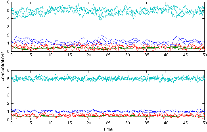
Assume that, for d = 1, Eq. (24) is the system under investigation that we observe. For 20 times 100 simulations of Eq. (24) with d = 1, X₁(0) = X_eq1 + 0.25, X₂(0) = X_eq2 + 0.25, X₃(0) = X_eq3 + 0.25, X₄(0) = 5.25 and stopped if either X₁ < 1.1, X₂ < 0.1, X₃ < 0.1, X₂ > 1, X₃ > 1 or X₁ ≥ 1.5, we observe that 1.95% of all runs, with a standard deviation of 1.43%, are terminated because of the latter. Let b(X) and σ be defined by Eq. (24). For P_m = 0.02 and d = 4, we solve the problem given by Eq. (9)–(14) using SOSTOOLS. (For brevity, we omit displaying the obtained function V (X).) We conclude from Theorem 1 that this implies that the model with d = 4 represents badly the data. Figure 3 shows three simulations of Eq. (24) for d = 1 and d = 4, where the dark blue line represents X₁ and the others the concentrations of X₂, X₃, and X₄. As expected, noise is much reduced for d = 4.

FIG. 3.

The top panel shows three simulations of Eq. (24) for d = 1 and the lower ones for d = 4, where the dark blue line represents X₁ and the others the concentrations of X₂, X₃, and X₄. As expected, noise is much reduced for d = 4.

4. Conclusions

The shortcomings of current experimental design approaches for discriminating between rival mathematical models representing a biological system are that they often use a linearized version of models or cannot deal well with experimental noise and parameter uncertainties. In this article, we presented novel means to computationally test a noisy nonlinear model by comparing it with measurement data of the system. Our approach is based on semidefinite programming techniques, for which efficient solvers exist. Importantly, our method provides analytical results and, thus, avoids extensive simulations. As opposed to analytical methods such as ours, numerical approaches can only approximate the (probabilistic) behavior of the model.

In the Results section, we provided examples of increasing complexity and finally applied our methodology to the Hog1 signaling pathway, a benchmark system, allowing the analysis of noise. Our approach is particularly useful to the field of systems biology, in which research thrives from the interaction between wet-lab work and mathematical modeling, and the models, often derived from data via reverse engineering, try to uncover structure and dynamics of biological systems.

Footnotes

Acknowledgment

This project was financed with a grant from the Swiss SystemsX.ch initiative (grant IPP-2011/115).

Disclosure Statement

No competing financial interests exist.

1

When noise in is intrinsic, it is also termed vanishing stochastic perturbations as then σ(0) = 0.

2

This assumption is important as it makes equal time-averaged results of single records with ensemble averaged results over many records (Bendat and Piersol, ).

3

However, our approach is not restricted to this type of criteria and allows also the implementation of many other kinds of stopping criteria, which we omit for clarity.

References

August

, Busch

2011. Efficient biological network determination with application to keratinocyte migration control. Presented at the 8th International Workshop on Computational Systems Biology, Zurich.

August

, Papachristodoulou

2009. A new computational tool for establishing model parameter identifiability. J. Comput. Biol., 16:875–884.

Behar

, Dohlman

H.G.

, Elston

T.C.

2007. Kinetic insulation as an effective mechanism for achieving pathway specificity in intracellular signaling networks. Proc. Natl. Acad. Sci. U.S.A., 104:16146–16151.

Bendat

J.S.

, Piersol

A.G.

2000. Random Data: Analysis and Measurement Procedures, 3rd. Wiley-Interscience: New York.

Boyd

, Vandenberghe

2004. Convex Optimization. Cambridge University Press: Cambridge, United Kingdom.

El-Samad

, Fazel

, Liu

et al. 2006a. Stochastic Reachability Analysis in Complex Biological Networks. Proc. Am. Control. Conf., 4748–4753.

El-Samad

, Khammash

2004. Stochastic stability and its application to the analysis of gene regulatory networks. Proc. Am. Control. Conf., 3001–3006.

El-Samad

, Prajna

, Papachristodoulou

et al. 2006b. advanced methods and algorithms for biological networks analysis. Proceedings of the IEEE, 94:832–853.

Elowitz

M.B.

, Levine

A.J.

, Siggia

E.D.

et al. 2002. Stochastic gene expression in a single cell. Science, 1183–1186.

10.

Feinberg

1987. Chemical reaction network structure and the stability of complex isothermal reactors–I. The deficiency zero and deficiency one theorems. Chem. Eng. Sci., 42:2229–2268.

11.

Gihman

I.I.

, Skorohod

A.V.

1972. Stochastic Differential Equations. Springer-Verlag: Berlin.

12.

Hohmann

, Krantz

, Nordlander

2007. Yeast osmoregulation. Meth. Enzymol., 428:29–45.

13.

Komorowski

, Finkenstädt

, Rand

2010. Using a single fluorescent reporter gene to infer half-life of extrinsic noise and other parameters of gene expression. Biophys. J., 98:2759–2769.

14.

Kushner

H.J.

1967. Stochastic Stability and Control. Academic Press: New York.

15.

Mélykúti

, August

, Papachristodoulou

et al. 2010. Discriminating between rival biochemical network models: three approaches to optimal experiment design. BMC Syst. Biol., 4:38.

16.

Munsky

, Trinh

, Khammash

2009. Listening to the noise: random fluctuations reveal gene network parameters. Mol. Syst. Biol., 5:318.

17.

Murty

K.G.

, Kabadi

S.N.

1987. Some NP-complete problems in quadratic and nonlinear programming. Math. Program, 39:117–129.

18.

Muzzey

, Gomez-Uribe

C.A.

, Mettetal

J.T.

et al. 2009. A systems-level analysis of perfect adaptation in yeast osmoregulation. Cell, 138:160–171.

19.

Øksendal

2003. Stochastic Differential Equation: An Introduction with Applications, 6th. Springer-Verlag: Berlin.

20.

Parrilo

P.A.

2003. Semidefinite programming relaxations for semialgebraic problems. Math. Program. Ser. B, 96:293–320.

21.

Prajna

, Jadbabaie

, Pappas

G.J.

2004. Stochastic safety verification using barrier certificates. Proc. IEEE Conf. Decis. Control, 929–934.

22.

Prajna

, Papachristodoulou

, Parrilo

P.A.

2002. SOSTOOLS: Sum of squares optimization toolbox for MATLAB. www.cds.caltech.edu/sostools. 2012 July 15.

23.

Roberts

, August

, Hamadeh

et al. 2009. A model invalidation-based approach for elucidating biological signalling pathways, applied to the chemotaxis pathway in R. sphaeroides. BMC Syst. Biol., 3:105.

24.

Schnell

, Turner

T.E.

2004. Reaction kinetics in intracellular environments with macromolecular crowding: simulations and rate laws. Prog. Biophys. Mol. Biol., 85:235–260.

25.

Shahrezaei

, Ollivier

J.F.

, Swain

P.S.

2008. Colored extrinsic fluctuations and stochastic gene expression. Mol. Syst. Biol., 4:196.

26.

Sotiropoulos

, Contou-Carrere

M.-N.

, Daoutidis

2009. Model reduction of multiscale chemical langevin equations: a numerical case study. IEEE/ACM Trans. Comput. Biol. Bioinform., 6:470–482.

27.

Sturm

J.F.

1999. Using SeDuMi 1.02, a MATLAB toolbox for optimization over symmetric cones. Optim. Methods. Softw., 11–12:625–653.

28.

Vandenberghe

, Boyd

1996. Semidefinite programming. SIAM Rev., 38:49–95.

29.

Ventsel’

A.D.

, Freidlin

M.I.

1970. On small random perturbations of dynamical systems. Russ. Math. Surv., 25:1.

30.

Westfall

P.J.

, Patterson

J.C.

, Chen

R.E.

et al. 2008. Stress resistance and signal fidelity independent of nuclear MAPK function. Proc. Natl. Acad. Sci. U.S.A., 105:12212–12217.