Accurate Estimations of Evolutionary Times in the Context of Strong CpG Hypermutability

Abstract

We consider the substitution model T92+CpG of DNA sequence evolution which takes into account the hypermutability of CpG dinucleotides, an effect that can be especially observed in vertebrate genomes. We provide an exact method to simulate the evolution of finite DNA sequences under this model and numerical procedures to infer evolutionary times in two cases: between an ancestral and a present sequence and between two homologous sequences. We show on simulated data that our new numerical method yields very accurate estimations of divergence times. In a context of strong CpG hypermutability, it clearly outperforms the classical estimation procedure that is solely based on the model T92 without CpG influence. Supplementary Material is available at www.liebertonline.com/cmb.

1. Introduction

The calculation of distances for DNA sequences remains an important part of molecular phylogenetics. For instance, the widely used algorithm PhyML developed by Guindon and Gascuel (2003) designed to estimate large phylogenies by maximum likelihood starts with a fast distance-based tree. More importantly, it is a useful tool to point out the strengths and weaknesses of Markov process models of nucleotide substitutions on which most of the phylogeny reconstruction methods are based. The present article should be viewed in light of this.

Most stochastic substitution models assume that nucleotide sites evolve independently from each other and, in general, according to a given Markovian kernel. Since the simplest model developed by Jukes and Cantor (1969), as well as other phylogeneticists such as Kimura (1980), Felsenstein (1981), Hasegawa et al. (1985), Tamura (1992), and Yang (1994) have incorporated more and more biological characteristics into substitution models to increase their accuracy. However, all these models still assume that there are no neighbor-dependencies between the different nucleotide sites. But this is actually not the case in a biological context. For instance, it is well known that, in vertebrate species, the frequency of the dinucleotide CpG is much lower than the product of C and G frequencies (Bird, 1980). The CpG deficiency is a consequence of the methylation of cytosine in CpG dinucleotides since methylated CpG dinucleotides may change into TpG with higher frequency and consequently into CpA on the complementary strand. For example, in a large-scale survey of the human genome, Wang et al. (1998) found that single-nucleotide polymorphisms are observed 10 times more often at CpGs than at other dinucleotides. Thus, incorporating the influence of the neighborhood into substitution models seems to be inevitable.

This is the reason why Duret and Galtier (2000) introduced a model that superimposes neighbor-dependent substitutions CpG → CpA and CpG → TpG onto Tamura's substitution rates, both at the additional rate r \documentclass{aastex}\usepackage{amsbsy}\usepackage{amsfonts}\usepackage{amssymb}\usepackage{bm}\usepackage{mathrsfs}\usepackage{pifont}\usepackage{stmaryrd}\usepackage{textcomp}\usepackage{portland, xspace}\usepackage{amsmath, amsxtra}\pagestyle{empty}\DeclareMathSizes{10}{9}{7}{6}\begin{document} $$\geqslant$$ \end{document} 0. Hereafter, this model will be denoted T92+CpG. However, introducing these neighbor-dependent substitution processes greatly complicates the inference of phylogenies and the estimation of divergence times: the distribution of a nucleotide at site i at a given time does not only depend on its value at previous times but also on the values of the surrounding sites i − 1 and i + 1 whose distributions in turn depend on the values at sites i − 2, i − 1, i, i + 1, and i + 2 at previous times and so on. Hence, one is faced with infinite-dimensional linear systems that are difficult to solve. To circumvent this problem, Duret and Galtier (2000) approximated trinucleotide frequencies (xyz) by dinucleotide frequencies (xy) in the following way: (xyz) ≈ (xy) (yz) / (y). Instead of relying on dinucleotide frequencies, Arndt and Hwa (2005) similarly assumed that word frequencies can be deduced from trinucleotide frequencies. However, all these approaches remain approximative and are not mathematically founded.

Entering the field of interacting particle systems (see Liggett [1985] for a review of the topic), Bérard et al. (2008) introduced a wide extension of the T92+CpG model of neighbor-dependent substitution processes, called RN+YpR, and investigated its theoretical properties. Thanks to the remarkable structural properties of this class of models, Bérard and Guéguen (2010) analyzed the performance of an original approach developed to show that the phylogenetic reconstruction methods in the context of independence between sites can be efficiently adapted to this class of models—within a mathematically rigorous framework and without resorting to approximations. They also compare their approach with the alternative strategy of Duret and Arndt (2008).

In the context of the Jukes Cantor model with CpG influence, i.e., the simplest but non-trivial model of the RN + YpR model class, Falconnet (2010a) provided theoretical estimation procedures for the time elapsed between an ancestral sequence at stationarity and a present one, and for the time of divergence between two homologous sequences that are originating from a common ancestral sequence at stationarity. For the ancestral case, Falconnet (2010a) showed that the result can be extended to the general RN + YpR models but he did not provide an explicit extension for the homologous case. The performance of these procedures has also not yet been investigated.

The goal of the present article is to derive theoretical estimation procedures for homologous sequences in the T92+CpG model. Furthermore, assuming model T92+CpG, we develop numerical solutions adapted from Falconnet (2010a) to estimate the time elapsed both between an ancestral and a present sequence and between two homologous sequences. Our numerical estimation procedures are evaluated on simulated data and are compared to the classical estimation method by Tamura (1992), which is based on the T92 model without CpG influence. It turns out that the classical estimators for evolution times become inaccurate very fast when the influence of the CpG hypermutability increases. In contrast, our new estimators based on model T92+CpG remain robust as soon as the hypermutability is significant. Thus, considering that CpG hypermutability is one of the major determinants driving the evolution of human DNA sequences, we can conclude that our new estimation procedure clearly outperforms the classical one.

The article is organized as follows. In Section 2, we describe the T92+CpG model, we explain how to simulate the evolution of DNA sequences under this model, we provide a method to infer phylogenetic distances for this neighbor-dependent model, and we describe our simulation experiment. In Section 3, we present our main results on the comparison of the two procedures to estimate the divergence time of two homologous DNA sequences. Section 4 is devoted to the discussion and impact of our findings. Further mathematical elaboration related to Section 2 and additional tables for the simulation experiments as available in Supplementary Material (available at www.liebertonline.com/cmb).

2. Methods

2.1. Description of the T92+CpG model

The T92+CpG model is a continuous-time model of DNA evolution where the sequences evolve under the combined effect of two superimposed mechanisms.

The first mechanism is an independent evolution of the sites, as in the classical T92 model developed by Tamura (1992). Hence, it is characterized by a 4 × 4 matrix of substitution rates, each rate being the mean number of substitutions per unit of time. In our case, the matrix is defined as

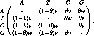
where v and w denote, respectively, the rates of transversional (T, C ↔ A, G) and transitional (T ↔ C or A ↔ G) changes and θ denotes the G+C content.

A second mechanism is superimposed that describes the substitutions due to the influence of the neighborhood: the most noticeable case is based on experimentally observed CpG-methylation-deamination processes. Hence, we assume that the substitution rates of cytosine by thymine and of guanine by adenine in CpG dinucleotides are both increased by an additional nonnegative rate r.

This means that every C site whose right neighbor is not occupied by a G (every G site whose left neighbor is not occupied by a C resp.) changes at global rate v + (1 − θ) w, i.e., after an exponentially distributed random time with mean 1 / [v + (1 − θ)w], and when it does, it becomes an A (a T resp.) with probability (1 − θ)v/[v + (1 − θ)w], a T (an A resp.) with probability (1 − θ)w/[v + (1 − θ)w], and a G (a C resp.) with probability θv/[v + (1 − θ)w]. On the contrary, every C site whose right neighbor is occupied by a G (every G site whose left neighbor is occupied by a C resp.) changes at global rate v + (1 − θ)w + r, i.e., after an exponentially distributed random time with mean 1 / [v + (1 − θ)w + r], and when it does, it becomes an A (a T resp.) with probability (1 − θ)v / [v + (1 − θ)w + r], a T (an A resp.) with probability [(1 − θ)w + r] / [v + (1 − θ)w + r], and a G (a C resp.) with probability θv / [v + (1 − θ)w + r].

The case r = 0 corresponds to the classical T92 model. We recall that the T92 + CpG model belongs to a larger class called RN + YpR introduced by Bérard et al. (2008), and we refer to this article for the main properties of the model.

2.2. Simulating the evolution of DNA sequences

Every model of the RN + YpR class can be constructed relying on the general principles based on infinitesimal generators described by Liggett (1985). However, Bérard et al. (2008) presented another construction based on Poisson processes called graphical representation, also developed by Liggett (1985), which is much more useful to simulate the evolution of a DNA sequence. We adapt this construction to our context.

In Falconnet (2010a), DNA sequences are presented as doubly infinite sequences of letters, i.e., elements of the set \documentclass{aastex}\usepackage{amsbsy}\usepackage{amsfonts}\usepackage{amssymb}\usepackage{bm}\usepackage{mathrsfs}\usepackage{pifont}\usepackage{stmaryrd}\usepackage{textcomp}\usepackage{portland, xspace}\usepackage{amsmath, amsxtra}\pagestyle{empty}\DeclareMathSizes{10}{9}{7}{6}\begin{document} $${\cal A}^{\mathbb Z}$$ \end{document} , where \documentclass{aastex}\usepackage{amsbsy}\usepackage{amsfonts}\usepackage{amssymb}\usepackage{bm}\usepackage{mathrsfs}\usepackage{pifont}\usepackage{stmaryrd}\usepackage{textcomp}\usepackage{portland, xspace}\usepackage{amsmath, amsxtra}\pagestyle{empty}\DeclareMathSizes{10}{9}{7}{6}\begin{document} $${\cal A} = \{A, T, C, G \}$$ \end{document} . Since real or simulated DNA sequences are obviously finite, we need to explain how to simulate the evolution of a finite sequence under a model developed for doubly infinite sequences. Thanks to mathematical properties presented in Bérard et al. (2008), we know that the behavior of the sites in \documentclass{aastex}\usepackage{amsbsy}\usepackage{amsfonts}\usepackage{amssymb}\usepackage{bm}\usepackage{mathrsfs}\usepackage{pifont}\usepackage{stmaryrd}\usepackage{textcomp}\usepackage{portland, xspace}\usepackage{amsmath, amsxtra}\pagestyle{empty}\DeclareMathSizes{10}{9}{7}{6}\begin{document} $$\{1, \ldots, N \}$$ \end{document} is the same regardless of whether one considers that these sites are embedded in a sequence indexed by \documentclass{aastex}\usepackage{amsbsy}\usepackage{amsfonts}\usepackage{amssymb}\usepackage{bm}\usepackage{mathrsfs}\usepackage{pifont}\usepackage{stmaryrd}\usepackage{textcomp}\usepackage{portland, xspace}\usepackage{amsmath, amsxtra}\pagestyle{empty}\DeclareMathSizes{10}{9}{7}{6}\begin{document} $${\mathbb Z}$$ \end{document} or in a sequence indexed by \documentclass{aastex}\usepackage{amsbsy}\usepackage{amsfonts}\usepackage{amssymb}\usepackage{bm}\usepackage{mathrsfs}\usepackage{pifont}\usepackage{stmaryrd}\usepackage{textcomp}\usepackage{portland, xspace}\usepackage{amsmath, amsxtra}\pagestyle{empty}\DeclareMathSizes{10}{9}{7}{6}\begin{document} $$\{0, 1, \ldots, N, N + 1 \}$$ \end{document} .

In our case, for a given sequence \documentclass{aastex}\usepackage{amsbsy}\usepackage{amsfonts}\usepackage{amssymb}\usepackage{bm}\usepackage{mathrsfs}\usepackage{pifont}\usepackage{stmaryrd}\usepackage{textcomp}\usepackage{portland, xspace}\usepackage{amsmath, amsxtra}\pagestyle{empty}\DeclareMathSizes{10}{9}{7}{6}\begin{document} $$X_{1:N}: = (X_1, \ldots, X_N)$$ \end{document} , where X_i is the value of the nucleotide at site i, we create a new sequence X_0:N+1 by adding two artificial nucleotides at sites 0 and N + 1. We know from Bérard et al. (2008) that the choice of the nucleotides we add in 0 and N + 1 will modify the evolution at the sites 0 and N + 1 but not at the sites \documentclass{aastex}\usepackage{amsbsy}\usepackage{amsfonts}\usepackage{amssymb}\usepackage{bm}\usepackage{mathrsfs}\usepackage{pifont}\usepackage{stmaryrd}\usepackage{textcomp}\usepackage{portland, xspace}\usepackage{amsmath, amsxtra}\pagestyle{empty}\DeclareMathSizes{10}{9}{7}{6}\begin{document} $$\{1, \ldots, N \}$$ \end{document} . With these two new nucleotides and the transformation of the interval as a circle, every site of the sequence possesses two neighbors.

It remains to describe how to simulate the evolution until a fixed time t of a circular sequence indexed by \documentclass{aastex}\usepackage{amsbsy}\usepackage{amsfonts}\usepackage{amssymb}\usepackage{bm}\usepackage{mathrsfs}\usepackage{pifont}\usepackage{stmaryrd}\usepackage{textcomp}\usepackage{portland, xspace}\usepackage{amsmath, amsxtra}\pagestyle{empty}\DeclareMathSizes{10}{9}{7}{6}\begin{document} $$\{0, 1, \ldots, N + 1 \}$$ \end{document} . For every site i in \documentclass{aastex}\usepackage{amsbsy}\usepackage{amsfonts}\usepackage{amssymb}\usepackage{bm}\usepackage{mathrsfs}\usepackage{pifont}\usepackage{stmaryrd}\usepackage{textcomp}\usepackage{portland, xspace}\usepackage{amsmath, amsxtra}\pagestyle{empty}\DeclareMathSizes{10}{9}{7}{6}\begin{document} $$\{0, 1, \ldots, N + 1 \}$$ \end{document} , we generate 10 independent homogeneous Poisson processes until time t with the labels, rates, and actions given in Table 1.

Table 1.

Labels, Rates and Actions of the Poisson Processes of the T92+CpG Model

Label	Rate	Action: The nucleotide at site i moves \documentclass{aastex}\usepackage{amsbsy}\usepackage{amsfonts}\usepackage{amssymb}\usepackage{bm}\usepackage{mathrsfs}\usepackage{pifont}\usepackage{stmaryrd}\usepackage{textcomp}\usepackage{portland, xspace}\usepackage{amsmath, amsxtra}\pagestyle{empty}\DeclareMathSizes{10}{9}{7}{6}\begin{document} $$\ldots$$ \end{document}
\documentclass{aastex}\usepackage{amsbsy}\usepackage{amsfonts}\usepackage{amssymb}\usepackage{bm}\usepackage{mathrsfs}\usepackage{pifont}\usepackage{stmaryrd}\usepackage{textcomp}\usepackage{portland, xspace}\usepackage{amsmath, amsxtra}\pagestyle{empty}\DeclareMathSizes{10}{9}{7}{6}\begin{document} $${\cal U}_i^A$$ \end{document}	(1 − θ)v	\documentclass{aastex}\usepackage{amsbsy}\usepackage{amsfonts}\usepackage{amssymb}\usepackage{bm}\usepackage{mathrsfs}\usepackage{pifont}\usepackage{stmaryrd}\usepackage{textcomp}\usepackage{portland, xspace}\usepackage{amsmath, amsxtra}\pagestyle{empty}\DeclareMathSizes{10}{9}{7}{6}\begin{document} $$\ldots$$ \end{document} unconditionally to A.
\documentclass{aastex}\usepackage{amsbsy}\usepackage{amsfonts}\usepackage{amssymb}\usepackage{bm}\usepackage{mathrsfs}\usepackage{pifont}\usepackage{stmaryrd}\usepackage{textcomp}\usepackage{portland, xspace}\usepackage{amsmath, amsxtra}\pagestyle{empty}\DeclareMathSizes{10}{9}{7}{6}\begin{document} $${\cal U}_i^T$$ \end{document}	(1 − θ)v	\documentclass{aastex}\usepackage{amsbsy}\usepackage{amsfonts}\usepackage{amssymb}\usepackage{bm}\usepackage{mathrsfs}\usepackage{pifont}\usepackage{stmaryrd}\usepackage{textcomp}\usepackage{portland, xspace}\usepackage{amsmath, amsxtra}\pagestyle{empty}\DeclareMathSizes{10}{9}{7}{6}\begin{document} $$\ldots$$ \end{document} unconditionally to T.
\documentclass{aastex}\usepackage{amsbsy}\usepackage{amsfonts}\usepackage{amssymb}\usepackage{bm}\usepackage{mathrsfs}\usepackage{pifont}\usepackage{stmaryrd}\usepackage{textcomp}\usepackage{portland, xspace}\usepackage{amsmath, amsxtra}\pagestyle{empty}\DeclareMathSizes{10}{9}{7}{6}\begin{document} $${\cal U}_i^C$$ \end{document}	θv	\documentclass{aastex}\usepackage{amsbsy}\usepackage{amsfonts}\usepackage{amssymb}\usepackage{bm}\usepackage{mathrsfs}\usepackage{pifont}\usepackage{stmaryrd}\usepackage{textcomp}\usepackage{portland, xspace}\usepackage{amsmath, amsxtra}\pagestyle{empty}\DeclareMathSizes{10}{9}{7}{6}\begin{document} $$\ldots$$ \end{document} unconditionally to C.
\documentclass{aastex}\usepackage{amsbsy}\usepackage{amsfonts}\usepackage{amssymb}\usepackage{bm}\usepackage{mathrsfs}\usepackage{pifont}\usepackage{stmaryrd}\usepackage{textcomp}\usepackage{portland, xspace}\usepackage{amsmath, amsxtra}\pagestyle{empty}\DeclareMathSizes{10}{9}{7}{6}\begin{document} $${\cal U}_i^G$$ \end{document}	θv	\documentclass{aastex}\usepackage{amsbsy}\usepackage{amsfonts}\usepackage{amssymb}\usepackage{bm}\usepackage{mathrsfs}\usepackage{pifont}\usepackage{stmaryrd}\usepackage{textcomp}\usepackage{portland, xspace}\usepackage{amsmath, amsxtra}\pagestyle{empty}\DeclareMathSizes{10}{9}{7}{6}\begin{document} $$\ldots$$ \end{document} unconditionally to G.
\documentclass{aastex}\usepackage{amsbsy}\usepackage{amsfonts}\usepackage{amssymb}\usepackage{bm}\usepackage{mathrsfs}\usepackage{pifont}\usepackage{stmaryrd}\usepackage{textcomp}\usepackage{portland, xspace}\usepackage{amsmath, amsxtra}\pagestyle{empty}\DeclareMathSizes{10}{9}{7}{6}\begin{document} $${\cal W}_i^A$$ \end{document}	(1 − θ)(w − v)	\documentclass{aastex}\usepackage{amsbsy}\usepackage{amsfonts}\usepackage{amssymb}\usepackage{bm}\usepackage{mathrsfs}\usepackage{pifont}\usepackage{stmaryrd}\usepackage{textcomp}\usepackage{portland, xspace}\usepackage{amsmath, amsxtra}\pagestyle{empty}\DeclareMathSizes{10}{9}{7}{6}\begin{document} $$\ldots$$ \end{document} to A provided that it is a G.
\documentclass{aastex}\usepackage{amsbsy}\usepackage{amsfonts}\usepackage{amssymb}\usepackage{bm}\usepackage{mathrsfs}\usepackage{pifont}\usepackage{stmaryrd}\usepackage{textcomp}\usepackage{portland, xspace}\usepackage{amsmath, amsxtra}\pagestyle{empty}\DeclareMathSizes{10}{9}{7}{6}\begin{document} $${\cal W}_i^T$$ \end{document}	(1 − θ)(w − v)	\documentclass{aastex}\usepackage{amsbsy}\usepackage{amsfonts}\usepackage{amssymb}\usepackage{bm}\usepackage{mathrsfs}\usepackage{pifont}\usepackage{stmaryrd}\usepackage{textcomp}\usepackage{portland, xspace}\usepackage{amsmath, amsxtra}\pagestyle{empty}\DeclareMathSizes{10}{9}{7}{6}\begin{document} $$\ldots$$ \end{document} to T provided that it is a C.
\documentclass{aastex}\usepackage{amsbsy}\usepackage{amsfonts}\usepackage{amssymb}\usepackage{bm}\usepackage{mathrsfs}\usepackage{pifont}\usepackage{stmaryrd}\usepackage{textcomp}\usepackage{portland, xspace}\usepackage{amsmath, amsxtra}\pagestyle{empty}\DeclareMathSizes{10}{9}{7}{6}\begin{document} $${\cal W}_i^C$$ \end{document}	θ(w − v)	\documentclass{aastex}\usepackage{amsbsy}\usepackage{amsfonts}\usepackage{amssymb}\usepackage{bm}\usepackage{mathrsfs}\usepackage{pifont}\usepackage{stmaryrd}\usepackage{textcomp}\usepackage{portland, xspace}\usepackage{amsmath, amsxtra}\pagestyle{empty}\DeclareMathSizes{10}{9}{7}{6}\begin{document} $$\ldots$$ \end{document} to C provided that it is a T.
\documentclass{aastex}\usepackage{amsbsy}\usepackage{amsfonts}\usepackage{amssymb}\usepackage{bm}\usepackage{mathrsfs}\usepackage{pifont}\usepackage{stmaryrd}\usepackage{textcomp}\usepackage{portland, xspace}\usepackage{amsmath, amsxtra}\pagestyle{empty}\DeclareMathSizes{10}{9}{7}{6}\begin{document} $${\cal W}_i^G$$ \end{document}	θ(w − v)	\documentclass{aastex}\usepackage{amsbsy}\usepackage{amsfonts}\usepackage{amssymb}\usepackage{bm}\usepackage{mathrsfs}\usepackage{pifont}\usepackage{stmaryrd}\usepackage{textcomp}\usepackage{portland, xspace}\usepackage{amsmath, amsxtra}\pagestyle{empty}\DeclareMathSizes{10}{9}{7}{6}\begin{document} $$\ldots$$ \end{document} to G provided that it is a A.
\documentclass{aastex}\usepackage{amsbsy}\usepackage{amsfonts}\usepackage{amssymb}\usepackage{bm}\usepackage{mathrsfs}\usepackage{pifont}\usepackage{stmaryrd}\usepackage{textcomp}\usepackage{portland, xspace}\usepackage{amsmath, amsxtra}\pagestyle{empty}\DeclareMathSizes{10}{9}{7}{6}\begin{document} $${\cal R}_i^T$$ \end{document}	r	\documentclass{aastex}\usepackage{amsbsy}\usepackage{amsfonts}\usepackage{amssymb}\usepackage{bm}\usepackage{mathrsfs}\usepackage{pifont}\usepackage{stmaryrd}\usepackage{textcomp}\usepackage{portland, xspace}\usepackage{amsmath, amsxtra}\pagestyle{empty}\DeclareMathSizes{10}{9}{7}{6}\begin{document} $$\ldots$$ \end{document} to T provided that it is a C and its right neighbor a G.
\documentclass{aastex}\usepackage{amsbsy}\usepackage{amsfonts}\usepackage{amssymb}\usepackage{bm}\usepackage{mathrsfs}\usepackage{pifont}\usepackage{stmaryrd}\usepackage{textcomp}\usepackage{portland, xspace}\usepackage{amsmath, amsxtra}\pagestyle{empty}\DeclareMathSizes{10}{9}{7}{6}\begin{document} $${\cal R}_i^A$$ \end{document}	r	\documentclass{aastex}\usepackage{amsbsy}\usepackage{amsfonts}\usepackage{amssymb}\usepackage{bm}\usepackage{mathrsfs}\usepackage{pifont}\usepackage{stmaryrd}\usepackage{textcomp}\usepackage{portland, xspace}\usepackage{amsmath, amsxtra}\pagestyle{empty}\DeclareMathSizes{10}{9}{7}{6}\begin{document} $$\ldots$$ \end{document} to A provided that it is a G and its left neighbor a C.

Depicted here are the labels, rates, and actions of the Poisson processes necessary to simulate the evolution of site i in a circular DNA sequence under the T92+CpG model.

Thus, we have 10 × (N + 2) independent homogeneous Poisson processes which run until time t. Let \documentclass{aastex}\usepackage{amsbsy}\usepackage{amsfonts}\usepackage{amssymb}\usepackage{bm}\usepackage{mathrsfs}\usepackage{pifont}\usepackage{stmaryrd}\usepackage{textcomp}\usepackage{portland, xspace}\usepackage{amsmath, amsxtra}\pagestyle{empty}\DeclareMathSizes{10}{9}{7}{6}\begin{document} $${\cal T} = (t_k)_{k = 0}^K$$ \end{document} denote the increasing list of random times generated by these random processes. We know that this list is almost surely finite, i.e., K < ∞, and that all the elements are almost surely pairwise distinct. Every time t_k in this list is associated with a site i_k and a label \documentclass{aastex}\usepackage{amsbsy}\usepackage{amsfonts}\usepackage{amssymb}\usepackage{bm}\usepackage{mathrsfs}\usepackage{pifont}\usepackage{stmaryrd}\usepackage{textcomp}\usepackage{portland, xspace}\usepackage{amsmath, amsxtra}\pagestyle{empty}\DeclareMathSizes{10}{9}{7}{6}\begin{document} $${\cal L}_{i_k}^{x_k}$$ \end{document} with \documentclass{aastex}\usepackage{amsbsy}\usepackage{amsfonts}\usepackage{amssymb}\usepackage{bm}\usepackage{mathrsfs}\usepackage{pifont}\usepackage{stmaryrd}\usepackage{textcomp}\usepackage{portland, xspace}\usepackage{amsmath, amsxtra}\pagestyle{empty}\DeclareMathSizes{10}{9}{7}{6}\begin{document} $${\cal L} \in \{{\cal U}, {\cal W}, {\cal R} \}$$ \end{document} . Hence, to simulate the evolution of the sequence, it suffices to read the list from t₀ to t_K and execute the action associated with site i_k and label \documentclass{aastex}\usepackage{amsbsy}\usepackage{amsfonts}\usepackage{amssymb}\usepackage{bm}\usepackage{mathrsfs}\usepackage{pifont}\usepackage{stmaryrd}\usepackage{textcomp}\usepackage{portland, xspace}\usepackage{amsmath, amsxtra}\pagestyle{empty}\DeclareMathSizes{10}{9}{7}{6}\begin{document} $${\cal L}_{i_k}^{x_k}$$ \end{document} .

The theory of Poisson Processes and the article from Bérard et al. (2008) suffice to prove that the simulation we provide matches the rates of the T92 + CpG model.

2.3. Inferring distances and asymptotic confidence intervals

In the estimation procedures below, both constructions are based on dinucleotides encoded in the alphabet \documentclass{aastex}\usepackage{amsbsy}\usepackage{amsfonts}\usepackage{amssymb}\usepackage{bm}\usepackage{mathrsfs}\usepackage{pifont}\usepackage{stmaryrd}\usepackage{textcomp}\usepackage{portland, xspace}\usepackage{amsmath, amsxtra}\pagestyle{empty}\DeclareMathSizes{10}{9}{7}{6}\begin{document} $${\cal B}$$ \end{document} defined as \documentclass{aastex}\usepackage{amsbsy}\usepackage{amsfonts}\usepackage{amssymb}\usepackage{bm}\usepackage{mathrsfs}\usepackage{pifont}\usepackage{stmaryrd}\usepackage{textcomp}\usepackage{portland, xspace}\usepackage{amsmath, amsxtra}\pagestyle{empty}\DeclareMathSizes{10}{9}{7}{6}\begin{document} \begin{align*} {\cal B} = \{R, T, C \} \times \{Y, A, G \}, \end{align*} \end{document}

where R denote the set of purines defined as {A, G} and Y the set of pyrimidines defined as {T, C}.

The estimators are based on various quantities provided by the alignment of the two sequences and we introduce some notations which are necessary for the rest of this section.

Notation 1

For every t, X(t) describes the whole sequence at time t and, for every i in \documentclass{aastex}\usepackage{amsbsy}\usepackage{amsfonts}\usepackage{amssymb}\usepackage{bm}\usepackage{mathrsfs}\usepackage{pifont}\usepackage{stmaryrd}\usepackage{textcomp}\usepackage{portland, xspace}\usepackage{amsmath, amsxtra}\pagestyle{empty}\DeclareMathSizes{10}{9}{7}{6}\begin{document} $${\mathbb Z}$$ \end{document} , the ith coordinate X_i(t) of X(t) is the random value of the nucleotide at site i and time t.

For every ℓ and every word w of length ℓ + 1 written in the alphabet \documentclass{aastex}\usepackage{amsbsy}\usepackage{amsfonts}\usepackage{amssymb}\usepackage{bm}\usepackage{mathrsfs}\usepackage{pifont}\usepackage{stmaryrd}\usepackage{textcomp}\usepackage{portland, xspace}\usepackage{amsmath, amsxtra}\pagestyle{empty}\DeclareMathSizes{10}{9}{7}{6}\begin{document} $${\cal A}$$ \end{document} , we say that site i is occupied by w at time t if and only if X_i:i+ℓ = w.

2.3.1. Ancestral case

The estimation procedure of the time elapsed between a present sequence and an ancestral one is based on the evolution of the quantity (C, C)(t), where (C, C)(t) denotes the frequency of sites occupied by C at time 0 (in the ancestral sequence) and by C at time t (in the present sequence) in doubly infinite DNA sequences.

Now, we recall from Falconnet (2010a) the definition of the estimator \documentclass{aastex}\usepackage{amsbsy}\usepackage{amsfonts}\usepackage{amssymb}\usepackage{bm}\usepackage{mathrsfs}\usepackage{pifont}\usepackage{stmaryrd}\usepackage{textcomp}\usepackage{portland, xspace}\usepackage{amsmath, amsxtra}\pagestyle{empty}\DeclareMathSizes{10}{9}{7}{6}\begin{document} $$(T_C^N)_{\rm est}$$ \end{document} of the elapsed time and the main results about this estimator.

Definition 2

where \documentclass{aastex}\usepackage{amsbsy}\usepackage{amsfonts}\usepackage{amssymb}\usepackage{bm}\usepackage{mathrsfs}\usepackage{pifont}\usepackage{stmaryrd}\usepackage{textcomp}\usepackage{portland, xspace}\usepackage{amsmath, amsxtra}\pagestyle{empty}\DeclareMathSizes{10}{9}{7}{6}\begin{document} $$(C, C)_{\rm obs}^N$$ \end{document} denotes the observed value of (C, C)(t) on aligned sequences of length N, i.e. \documentclass{aastex}\usepackage{amsbsy}\usepackage{amsfonts}\usepackage{amssymb}\usepackage{bm}\usepackage{mathrsfs}\usepackage{pifont}\usepackage{stmaryrd}\usepackage{textcomp}\usepackage{portland, xspace}\usepackage{amsmath, amsxtra}\pagestyle{empty}\DeclareMathSizes{10}{9}{7}{6}\begin{document} \begin{align*} (C, C)_{\rm obs}^N = \frac {1} {N} \sum_{i = 1}^N {\bf 1} \{ X_i (0) = X_i (t) = C \} . \end{align*} \end{document}

Let \documentclass{aastex}\usepackage{amsbsy}\usepackage{amsfonts}\usepackage{amssymb}\usepackage{bm}\usepackage{mathrsfs}\usepackage{pifont}\usepackage{stmaryrd}\usepackage{textcomp}\usepackage{portland, xspace}\usepackage{amsmath, amsxtra}\pagestyle{empty}\DeclareMathSizes{10}{9}{7}{6}\begin{document} $$(\kappa_C^N)_{\rm obs}$$ \end{document} and \documentclass{aastex}\usepackage{amsbsy}\usepackage{amsfonts}\usepackage{amssymb}\usepackage{bm}\usepackage{mathrsfs}\usepackage{pifont}\usepackage{stmaryrd}\usepackage{textcomp}\usepackage{portland, xspace}\usepackage{amsmath, amsxtra}\pagestyle{empty}\DeclareMathSizes{10}{9}{7}{6}\begin{document} $$(V_C^N)_{\rm obs}$$ \end{document} denote the quantities defined as \documentclass{aastex}\usepackage{amsbsy}\usepackage{amsfonts}\usepackage{amssymb}\usepackage{bm}\usepackage{mathrsfs}\usepackage{pifont}\usepackage{stmaryrd}\usepackage{textcomp}\usepackage{portland, xspace}\usepackage{amsmath, amsxtra}\pagestyle{empty}\DeclareMathSizes{10}{9}{7}{6}\begin{document} \begin{align*} (\kappa_C^N)_{\rm obs} & = - \theta v (C, R)_{\rm obs}^N - \theta w (C, T)_{\rm obs}^N + [ v + (1 - \theta) w ] (C, C)_{\rm obs}^N + r (C *, CG)_{\rm obs}^N, \\ (\nu_C^N)_{\rm obs} & = (C, C)_{\rm obs}^N - 5 (C, C)_{\rm obs}^N {}^2 + 2 (CC, CC)_{\rm obs}^N + 2 (C*C, C*C)_{\rm obs}^N. \end{align*} \end{document}

Then we have that \documentclass{aastex}\usepackage{amsbsy}\usepackage{amsfonts}\usepackage{amssymb}\usepackage{bm}\usepackage{mathrsfs}\usepackage{pifont}\usepackage{stmaryrd}\usepackage{textcomp}\usepackage{portland, xspace}\usepackage{amsmath, amsxtra}\pagestyle{empty}\DeclareMathSizes{10}{9}{7}{6}\begin{document} \begin{align*} (\kappa_C^N)_{\rm obs} \mathop {\longrightarrow} \limits_{N \to \infty}^{a.s.} - (C, C)^{\prime} (t) . \end{align*} \end{document}

It originates from the delta method used in Falconnet (2010a). The quantity \documentclass{aastex}\usepackage{amsbsy}\usepackage{amsfonts}\usepackage{amssymb}\usepackage{bm}\usepackage{mathrsfs}\usepackage{pifont}\usepackage{stmaryrd}\usepackage{textcomp}\usepackage{portland, xspace}\usepackage{amsmath, amsxtra}\pagestyle{empty}\DeclareMathSizes{10}{9}{7}{6}\begin{document} $$(\nu_C^N)_{\rm obs}$$ \end{document} is the variance of \documentclass{aastex}\usepackage{amsbsy}\usepackage{amsfonts}\usepackage{amssymb}\usepackage{bm}\usepackage{mathrsfs}\usepackage{pifont}\usepackage{stmaryrd}\usepackage{textcomp}\usepackage{portland, xspace}\usepackage{amsmath, amsxtra}\pagestyle{empty}\DeclareMathSizes{10}{9}{7}{6}\begin{document} $$(C, C)_{\rm obs}^N$$ \end{document} .

Theorem 3

(Falconnet, 2010a). Assume that the function t ↦ (C, C)(t) is a diffeomorphism and that the ancestral sequence is at stationarity. Then, when N → ∞, \documentclass{aastex}\usepackage{amsbsy}\usepackage{amsfonts}\usepackage{amssymb}\usepackage{bm}\usepackage{mathrsfs}\usepackage{pifont}\usepackage{stmaryrd}\usepackage{textcomp}\usepackage{portland, xspace}\usepackage{amsmath, amsxtra}\pagestyle{empty}\DeclareMathSizes{10}{9}{7}{6}\begin{document} \begin{align*} (T_C^N)_{\rm est} \mathop {\longrightarrow} \limits^{a.s} t \ and \ (\kappa_C^N)_{\rm obs} \sqrt{N / (\nu_C^N)_{\rm obs}} \ [ (T_C^N)_{\rm est} - t ] \mathop {\longrightarrow} \limits^{d.} {\cal N} (0, 1), \end{align*} \end{document}

where \documentclass{aastex}\usepackage{amsbsy}\usepackage{amsfonts}\usepackage{amssymb}\usepackage{bm}\usepackage{mathrsfs}\usepackage{pifont}\usepackage{stmaryrd}\usepackage{textcomp}\usepackage{portland, xspace}\usepackage{amsmath, amsxtra}\pagestyle{empty}\DeclareMathSizes{10}{9}{7}{6}\begin{document} $${\cal N} (0, 1)$$ \end{document} denotes the standard normal law. An asymptotic confidence interval at level ɛ for t is given by \documentclass{aastex}\usepackage{amsbsy}\usepackage{amsfonts}\usepackage{amssymb}\usepackage{bm}\usepackage{mathrsfs}\usepackage{pifont}\usepackage{stmaryrd}\usepackage{textcomp}\usepackage{portland, xspace}\usepackage{amsmath, amsxtra}\pagestyle{empty}\DeclareMathSizes{10}{9}{7}{6}\begin{document} \begin{align*} \left[ (T_C^N)_{\rm est} - \frac {z (\varepsilon)} {(\kappa_C^N)_{\rm obs}} \sqrt {\frac {(\nu_C^N)_{\rm obs}} {N}}, (T_C^N)_{\rm est} + \frac {z (\varepsilon)} {(\kappa_C^N)_{\rm obs}} \sqrt {\frac {(\nu_C^N)_{\rm obs}} {N}} \right], \end{align*} \end{document}

where z(ɛ) denotes the unique real number such that \documentclass{aastex}\usepackage{amsbsy}\usepackage{amsfonts}\usepackage{amssymb}\usepackage{bm}\usepackage{mathrsfs}\usepackage{pifont}\usepackage{stmaryrd}\usepackage{textcomp}\usepackage{portland, xspace}\usepackage{amsmath, amsxtra}\pagestyle{empty}\DeclareMathSizes{10}{9}{7}{6}\begin{document} $${\mathbb P} (|Z| \geqslant z (\varepsilon)) = \varepsilon$$ \end{document} with \documentclass{aastex}\usepackage{amsbsy}\usepackage{amsfonts}\usepackage{amssymb}\usepackage{bm}\usepackage{mathrsfs}\usepackage{pifont}\usepackage{stmaryrd}\usepackage{textcomp}\usepackage{portland, xspace}\usepackage{amsmath, amsxtra}\pagestyle{empty}\DeclareMathSizes{10}{9}{7}{6}\begin{document} $$Z \sim {\cal N} (0, 1)$$ \end{document} .

From Theorem 3, we can compute an estimator of the time elapsed provided that we are able to solve equation (1). To bypass this difficulty, we use the classical Runge-Kutta method (RK4). The RK4 method is an iterative method for the approximation of solutions of ordinary differential equations (Butcher, 2008). In Supplementary Material A.2.1, we explain the algorithm we use (see online Supplementary Material at www.liebertonline.com/cmb).

2.3.2. Homologous case

The estimation procedure of the time from divergence for two homologous sequences originating from a common ancestral sequence at stationarity is based on the evolution of the quantity [C, C](t), where [C, C](t) denotes the frequency of sites occupied by a C at time t in both doubly infinite present sequences. Similarly to the ancestral case, the definition of the estimator \documentclass{aastex}\usepackage{amsbsy}\usepackage{amsfonts}\usepackage{amssymb}\usepackage{bm}\usepackage{mathrsfs}\usepackage{pifont}\usepackage{stmaryrd}\usepackage{textcomp}\usepackage{portland, xspace}\usepackage{amsmath, amsxtra}\pagestyle{empty}\DeclareMathSizes{10}{9}{7}{6}\begin{document} $$[ T_C^N ]_{\rm est}$$ \end{document} of the divergence time is as follows:

Definition 4

where \documentclass{aastex}\usepackage{amsbsy}\usepackage{amsfonts}\usepackage{amssymb}\usepackage{bm}\usepackage{mathrsfs}\usepackage{pifont}\usepackage{stmaryrd}\usepackage{textcomp}\usepackage{portland, xspace}\usepackage{amsmath, amsxtra}\pagestyle{empty}\DeclareMathSizes{10}{9}{7}{6}\begin{document} $$[ C, C ]_{\rm obs}^N$$ \end{document} denotes the observed value of [C, C](t) of the aligned present sequences X¹ and X² of length N, i.e., \documentclass{aastex}\usepackage{amsbsy}\usepackage{amsfonts}\usepackage{amssymb}\usepackage{bm}\usepackage{mathrsfs}\usepackage{pifont}\usepackage{stmaryrd}\usepackage{textcomp}\usepackage{portland, xspace}\usepackage{amsmath, amsxtra}\pagestyle{empty}\DeclareMathSizes{10}{9}{7}{6}\begin{document} \begin{align*} [ C, C ]_{\rm obs}^N = \frac {1} {N} \sum_{i = 1}^N {\bf 1} \{X_i^1 (t) = X_i^2 (t) = C \} . \end{align*} \end{document}

Let \documentclass{aastex}\usepackage{amsbsy}\usepackage{amsfonts}\usepackage{amssymb}\usepackage{bm}\usepackage{mathrsfs}\usepackage{pifont}\usepackage{stmaryrd}\usepackage{textcomp}\usepackage{portland, xspace}\usepackage{amsmath, amsxtra}\pagestyle{empty}\DeclareMathSizes{10}{9}{7}{6}\begin{document} $$[ \kappa_C^N ]_{\rm obs}$$ \end{document} and \documentclass{aastex}\usepackage{amsbsy}\usepackage{amsfonts}\usepackage{amssymb}\usepackage{bm}\usepackage{mathrsfs}\usepackage{pifont}\usepackage{stmaryrd}\usepackage{textcomp}\usepackage{portland, xspace}\usepackage{amsmath, amsxtra}\pagestyle{empty}\DeclareMathSizes{10}{9}{7}{6}\begin{document} $$[ \nu_C^N ]_{\rm obs}$$ \end{document} denote the quantities defined as \documentclass{aastex}\usepackage{amsbsy}\usepackage{amsfonts}\usepackage{amssymb}\usepackage{bm}\usepackage{mathrsfs}\usepackage{pifont}\usepackage{stmaryrd}\usepackage{textcomp}\usepackage{portland, xspace}\usepackage{amsmath, amsxtra}\pagestyle{empty}\DeclareMathSizes{10}{9}{7}{6}\begin{document} \begin{align*} [ \kappa_C^N ]_{\rm obs} & = - \sum_{(uv, xy) \in {\cal B} \times {\cal B}} Q_{\rm hom} ([ uv, xy ], [ u^{\prime}v^{\prime}, x^{\prime}y^{\prime} ]) \ [ uv, xy ]_{\rm obs}, \\ [ \nu_C^N ]_{\rm obs} & = [ C, C ]_{\rm obs}^N - 5 [ C, C ]_{\rm obs}^{N{\,}^2} + 2 [ CC, CC ]_{\rm obs}^N + 2 [ C*C, C*C ]_{\rm obs}^N. \end{align*} \end{document}

The matrix Q_hom is defined in Supplementary Material A.2.2 (see online Supplementary Material at www.liebertonline.com/cmb). Analogously to the ancestral case, we have that \documentclass{aastex}\usepackage{amsbsy}\usepackage{amsfonts}\usepackage{amssymb}\usepackage{bm}\usepackage{mathrsfs}\usepackage{pifont}\usepackage{stmaryrd}\usepackage{textcomp}\usepackage{portland, xspace}\usepackage{amsmath, amsxtra}\pagestyle{empty}\DeclareMathSizes{10}{9}{7}{6}\begin{document} \begin{align*} [ \kappa_C^N ]_{\rm obs} \mathop{\longrightarrow} \limits_{N \to \infty}^{a.s.} - [ C, C ]^{\prime} (t). \end{align*} \end{document}

Theorem 5

(Falconnet, 2010b). Assume that the function t ↦ [C, C](t) is a diffeomorphism and that the ancestral sequence is at stationarity. Then, when N → ∞, \documentclass{aastex}\usepackage{amsbsy}\usepackage{amsfonts}\usepackage{amssymb}\usepackage{bm}\usepackage{mathrsfs}\usepackage{pifont}\usepackage{stmaryrd}\usepackage{textcomp}\usepackage{portland, xspace}\usepackage{amsmath, amsxtra}\pagestyle{empty}\DeclareMathSizes{10}{9}{7}{6}\begin{document} \begin{align*} [ T_C^N ]_{\rm est} \mathop{\longrightarrow} \limits^{a.s} \ t \quad and \quad [ \kappa_C^N ]_{\rm obs} \sqrt{N / [ \nu_C^N ]_{\rm obs}} [ [ T_C^N ]_{\rm est} - t ] \mathop{\longrightarrow} \limits^{d.} {\cal N} (0, 1), \end{align*} \end{document}

where \documentclass{aastex}\usepackage{amsbsy}\usepackage{amsfonts}\usepackage{amssymb}\usepackage{bm}\usepackage{mathrsfs}\usepackage{pifont}\usepackage{stmaryrd}\usepackage{textcomp}\usepackage{portland, xspace}\usepackage{amsmath, amsxtra}\pagestyle{empty}\DeclareMathSizes{10}{9}{7}{6}\begin{document} $${\cal N} (0, 1)$$ \end{document} denotes the standard normal law. An asymptotic confidence interval at level ɛ for t is given by \documentclass{aastex}\usepackage{amsbsy}\usepackage{amsfonts}\usepackage{amssymb}\usepackage{bm}\usepackage{mathrsfs}\usepackage{pifont}\usepackage{stmaryrd}\usepackage{textcomp}\usepackage{portland, xspace}\usepackage{amsmath, amsxtra}\pagestyle{empty}\DeclareMathSizes{10}{9}{7}{6}\begin{document} \begin{align*} \left[ [ T_C^N ]_{\rm est} - \frac {z (\varepsilon)} {[ \kappa_C^N ]_{\rm obs}} \sqrt {\frac {[ \nu_C^N ]_{\rm obs}} {N}}, [ T_C^N ]_{\rm est} + \frac {z (\varepsilon)} {[ \kappa_C^N ]_{\rm obs}} \sqrt {\frac {[ \nu_C^N ]_{\rm obs}} {N}} \right], \end{align*} \end{document}

where z(ɛ) denotes the unique real number such that \documentclass{aastex}\usepackage{amsbsy}\usepackage{amsfonts}\usepackage{amssymb}\usepackage{bm}\usepackage{mathrsfs}\usepackage{pifont}\usepackage{stmaryrd}\usepackage{textcomp}\usepackage{portland, xspace}\usepackage{amsmath, amsxtra}\pagestyle{empty}\DeclareMathSizes{10}{9}{7}{6}\begin{document} $${\mathbb P} (\mid Z \mid \geqslant z (\varepsilon)) = \varepsilon$$ \end{document} with \documentclass{aastex}\usepackage{amsbsy}\usepackage{amsfonts}\usepackage{amssymb}\usepackage{bm}\usepackage{mathrsfs}\usepackage{pifont}\usepackage{stmaryrd}\usepackage{textcomp}\usepackage{portland, xspace}\usepackage{amsmath, amsxtra}\pagestyle{empty}\DeclareMathSizes{10}{9}{7}{6}\begin{document} $$Z \sim {\cal N} (0, 1)$$ \end{document} .

Using Theorem 5, we can obtain an estimator of the divergence time of two homologous sequences if we are able to solve equation (2). In order to do so, as in the ancestral case, we use the classical Runge-Kutta method (RK4) (see Supplementary Material A.2.2, available at www.liebertonline.com/cmb).

2.4. Simulation experiment: comparing estimation procedures

For all our simulations, we have focused on the T92+CpG model with parameters v = 1, w = 3, θ = 0.4 and several different values for the parameter r. The set of parameters (v, w, θ) is always assumed to be the same since we are only interested in the influence of the CpG hypermutability effect (specified by the parameter r) on the quality of the estimation procedures. The choice of parameters will be also discussed in Section 4.

In each case, the functions t ↦ (C, C)(t) and t ↦ [C, C](t) are diffeomorphisms as explained in Supplementary Material A.1 (available at www.liebertonline.com/cmb) Thus, the conditions for Theorems 3 and 5 are fulfilled and the estimators \documentclass{aastex}\usepackage{amsbsy}\usepackage{amsfonts}\usepackage{amssymb}\usepackage{bm}\usepackage{mathrsfs}\usepackage{pifont}\usepackage{stmaryrd}\usepackage{textcomp}\usepackage{portland, xspace}\usepackage{amsmath, amsxtra}\pagestyle{empty}\DeclareMathSizes{10}{9}{7}{6}\begin{document} $$(T_C^N)_{\rm est}$$ \end{document} and \documentclass{aastex}\usepackage{amsbsy}\usepackage{amsfonts}\usepackage{amssymb}\usepackage{bm}\usepackage{mathrsfs}\usepackage{pifont}\usepackage{stmaryrd}\usepackage{textcomp}\usepackage{portland, xspace}\usepackage{amsmath, amsxtra}\pagestyle{empty}\DeclareMathSizes{10}{9}{7}{6}\begin{document} $$[ T_C^N ]_{\rm est}$$ \end{document} can be obtained by applying the Runge-Kutta method (RK4) (see Supplementary Material A.2.1 and A.2.2, available at www.liebertonline.com/cmb).

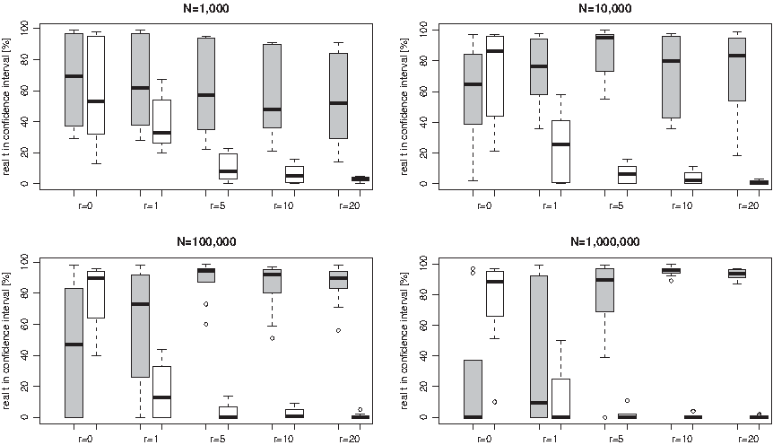
Employing the tool “random sequence” from the RSAT suite with independent and equiprobable nucleotides, we generated random DNA sequences of length N = 1000, 10,000, 100,000 and 1,000,000 bp (Thomas-Chollier et al., 2008). In order to obtain a DNA sequence at stationarity according to the T92+CpG model with parameters v = 1, w = 3, θ = 0.4 and r = 10, we wrote a Python script simulating the evolution of a given random sequence until time t = 2 as described in Section 2.2. This should suffice to produce stationary DNA sequences. As to be expected at stationarity, the resulting DNA sequences at time t = 2 contain 32.4% As, 32.4% Ts, 17.6% Cs, and 17.6% Ts, and the CpG content is 0.96%. In the following, we only used these stationary sequences as ancestral DNA sequences for the subsequent simulations.

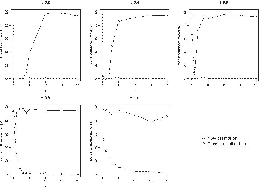
Starting from every of these stationary ancestral DNA sequences, we then simulated its evolution until various time points t for different values of r, r = 0,0.1,1,2,3,4,5,10,15 and 20, according to the T92+CpG model with parameters v = 1, w = 3 and θ = 0.4 (see Section 2.2). Each simulation has been carried out 100 times.

Our aim is to compare the results of our estimation procedure as described in Sections 2.3.1 and 2.3.2 to a classical estimation procedure of divergence times that is based on the T92 model without CpG influence by Tamura (1992) on the simulated data. The classical estimation procedure according to Tamura (1992) is described in Supplementary Material A.3 (available at www.liebertonline.com/cmb). Let \documentclass{aastex}\usepackage{amsbsy}\usepackage{amsfonts}\usepackage{amssymb}\usepackage{bm}\usepackage{mathrsfs}\usepackage{pifont}\usepackage{stmaryrd}\usepackage{textcomp}\usepackage{portland, xspace}\usepackage{amsmath, amsxtra}\pagestyle{empty}\DeclareMathSizes{10}{9}{7}{6}\begin{document} $$(T_{\rm Tamura}^N)_{\rm est}$$ \end{document} and \documentclass{aastex}\usepackage{amsbsy}\usepackage{amsfonts}\usepackage{amssymb}\usepackage{bm}\usepackage{mathrsfs}\usepackage{pifont}\usepackage{stmaryrd}\usepackage{textcomp}\usepackage{portland, xspace}\usepackage{amsmath, amsxtra}\pagestyle{empty}\DeclareMathSizes{10}{9}{7}{6}\begin{document} $$[ T_{\rm Tamura}^N ]_{\rm est}$$ \end{document} as defined in the Supplementary Material (see equations (6) and (7)) denote the classical estimators according to Tamura (1992) for the divergence time between an ancestral and a present sequence and between two homologous sequences respectiveley.

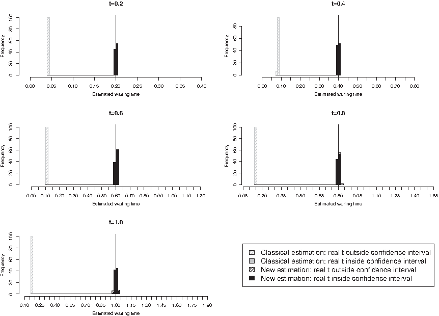
In the first scenario, we compared the evolved sequence X(t) at time t, t ranging from 0.1 to 1.0, to the ancestral DNA sequence X(0) and estimated the time elapsed between the two sequences using two different estimators: (i) our estimator \documentclass{aastex}\usepackage{amsbsy}\usepackage{amsfonts}\usepackage{amssymb}\usepackage{bm}\usepackage{mathrsfs}\usepackage{pifont}\usepackage{stmaryrd}\usepackage{textcomp}\usepackage{portland, xspace}\usepackage{amsmath, amsxtra}\pagestyle{empty}\DeclareMathSizes{10}{9}{7}{6}\begin{document} $$(T_C^N)_{\rm est}$$ \end{document} based on model T92+CpG as described in Section 2.3.1, and (ii) the classical estimator \documentclass{aastex}\usepackage{amsbsy}\usepackage{amsfonts}\usepackage{amssymb}\usepackage{bm}\usepackage{mathrsfs}\usepackage{pifont}\usepackage{stmaryrd}\usepackage{textcomp}\usepackage{portland, xspace}\usepackage{amsmath, amsxtra}\pagestyle{empty}\DeclareMathSizes{10}{9}{7}{6}\begin{document} $$(T_{\rm Tamura}^N)_{\rm est}$$ \end{document} 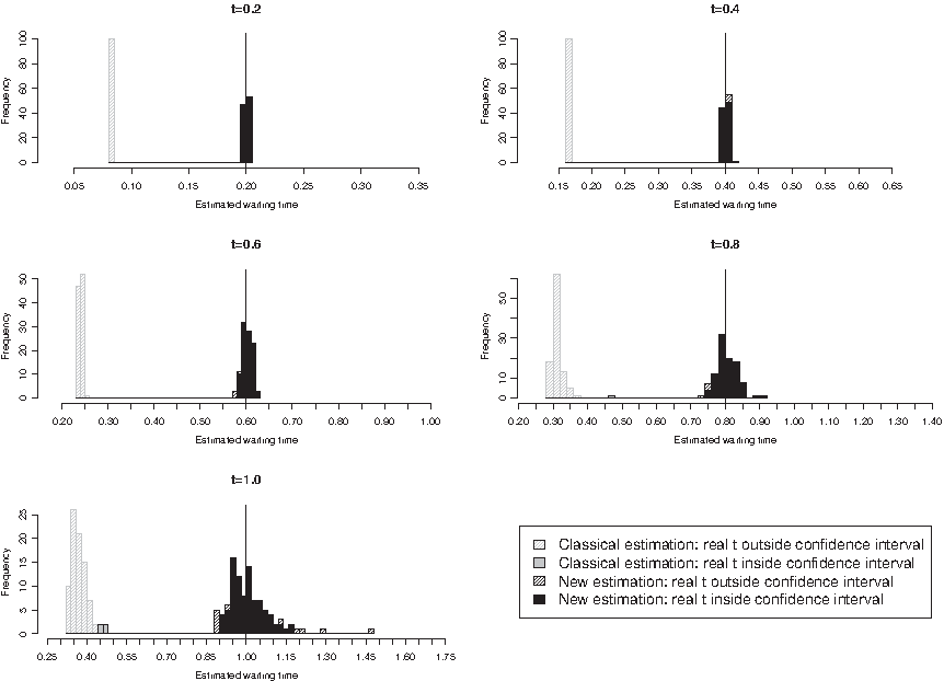for model T92 according to Tamura (1992). In the second scenario, we let the ancestral sequence X(0) evolve twice until time t and, for every time point t, t ranging from 0.1 to 1.0, compared the two resulting homologous sequences X¹(t) and X²(t) to each other. As in the first scenario, we then estimated the divergence time between these two homologous sequences by (i) \documentclass{aastex}\usepackage{amsbsy}\usepackage{amsfonts}\usepackage{amssymb}\usepackage{bm}\usepackage{mathrsfs}\usepackage{pifont}\usepackage{stmaryrd}\usepackage{textcomp}\usepackage{portland, xspace}\usepackage{amsmath, amsxtra}\pagestyle{empty}\DeclareMathSizes{10}{9}{7}{6}\begin{document} $$[ T_C^N ]_{\rm est}$$ \end{document} and by (ii) \documentclass{aastex}\usepackage{amsbsy}\usepackage{amsfonts}\usepackage{amssymb}\usepackage{bm}\usepackage{mathrsfs}\usepackage{pifont}\usepackage{stmaryrd}\usepackage{textcomp}\usepackage{portland, xspace}\usepackage{amsmath, amsxtra}\pagestyle{empty}\DeclareMathSizes{10}{9}{7}{6}\begin{document} $$[ T_{\rm Tamura}^N ]_{\rm est}$$ \end{document} . In both scenarios, we additionally computed the 95% asymptotic confidence intervals of all the estimators based on the estimation method that has been employed, i.e., of \documentclass{aastex}\usepackage{amsbsy}\usepackage{amsfonts}\usepackage{amssymb}\usepackage{bm}\usepackage{mathrsfs}\usepackage{pifont}\usepackage{stmaryrd}\usepackage{textcomp}\usepackage{portland, xspace}\usepackage{amsmath, amsxtra}\pagestyle{empty}\DeclareMathSizes{10}{9}{7}{6}\begin{document} $$(T_C^N)_{\rm est}$$ \end{document} and \documentclass{aastex}\usepackage{amsbsy}\usepackage{amsfonts}\usepackage{amssymb}\usepackage{bm}\usepackage{mathrsfs}\usepackage{pifont}\usepackage{stmaryrd}\usepackage{textcomp}\usepackage{portland, xspace}\usepackage{amsmath, amsxtra}\pagestyle{empty}\DeclareMathSizes{10}{9}{7}{6}\begin{document} $$[ T_C^N ]_{\rm est}$$ \end{document} according to Theorems 3 and 5 and of \documentclass{aastex}\usepackage{amsbsy}\usepackage{amsfonts}\usepackage{amssymb}\usepackage{bm}\usepackage{mathrsfs}\usepackage{pifont}\usepackage{stmaryrd}\usepackage{textcomp}\usepackage{portland, xspace}\usepackage{amsmath, amsxtra}\pagestyle{empty}\DeclareMathSizes{10}{9}{7}{6}\begin{document} $$(T_{\rm Tamura}^N)_{\rm est}$$ \end{document} and \documentclass{aastex}\usepackage{amsbsy}\usepackage{amsfonts}\usepackage{amssymb}\usepackage{bm}\usepackage{mathrsfs}\usepackage{pifont}\usepackage{stmaryrd}\usepackage{textcomp}\usepackage{portland, xspace}\usepackage{amsmath, amsxtra}\pagestyle{empty}\DeclareMathSizes{10}{9}{7}{6}\begin{document} $$[ T_{\rm Tamura}^N ]_{\rm est}$$ \end{document} according to Supplementary Material A.3, equations (8) and (9) (see online Supplementary Material at www.liebertonline.com/cmb). Finally, we checked whether the real t lies within this interval. We then used the percentage of real t lying in the confidence interval to assess the quality of the two estimation procedures.

When estimating the 95% asymptotic confidence interval for homologous sequences according to our estimation procedure, in some cases, especially when the sequence length N is small, \documentclass{aastex}\usepackage{amsbsy}\usepackage{amsfonts}\usepackage{amssymb}\usepackage{bm}\usepackage{mathrsfs}\usepackage{pifont}\usepackage{stmaryrd}\usepackage{textcomp}\usepackage{portland, xspace}\usepackage{amsmath, amsxtra}\pagestyle{empty}\DeclareMathSizes{10}{9}{7}{6}\begin{document} $$[ \kappa_C^N ]_{\rm obs}$$ \end{document} can be negative resulting in a negative asymptotic variance (see Theorem 5). In this case, the 95%-confidence interval is not defined. Thus, for further analyses, we have filtered out these cases (for example, for r = 10 we had to filter out 25.4% of the estimations for N = 1,000 bp, 15.6% for N = 10,000 bp, 7.1% for N = 100,000 bp, and only 0.5% for N = 1,000,000 bp). On the other hand, when estimating the divergence time between homologous sequences according to the classical estimation procedure, in some cases, especially when t is large, the estimator \documentclass{aastex}\usepackage{amsbsy}\usepackage{amsfonts}\usepackage{amssymb}\usepackage{bm}\usepackage{mathrsfs}\usepackage{pifont}\usepackage{stmaryrd}\usepackage{textcomp}\usepackage{portland, xspace}\usepackage{amsmath, amsxtra}\pagestyle{empty}\DeclareMathSizes{10}{9}{7}{6}\begin{document} $$[ T_{\rm Tamura}^N ]_{\rm est}$$ \end{document} is not well defined either (in equation (5), \documentclass{aastex}\usepackage{amsbsy}\usepackage{amsfonts}\usepackage{amssymb}\usepackage{bm}\usepackage{mathrsfs}\usepackage{pifont}\usepackage{stmaryrd}\usepackage{textcomp}\usepackage{portland, xspace}\usepackage{amsmath, amsxtra}\pagestyle{empty}\DeclareMathSizes{10}{9}{7}{6}\begin{document} $$1 - \frac {\hat {p}} {\theta_1 + \theta_2 - 2 \theta_1 \theta_2} - \hat {q}$$ \end{document} can be negative). We have also filtered out these cases (for example, for r = 10, 31.3% of the estimations had to be filtered out for N = 1,000 bp, 16.4% for N = 10,000 bp, 9.9% for N = 100,000 bp, and 2.5% for N = 1,000,000 bp).

3. Results

In this section, we assess the performance of the two distinct methods we consider for estimating evolutionary times, i.e., of our estimation procedure (see Sections 2.3 and 2.4) and of the classical estimation method based on the T92 model without CpG influence by Tamura (1992) (see Section 2.4 and Supplementary Material A.3, available at www.liebertonline.com/cmb). We mainly focus on the homologous case and only briefly deal with the ancestral case. We assess the impact of the CpG hypermutability effects on the accuracy of the estimation procedures and the impact of the sequence length on the size of the confidence interval computed.

3.1. In the ancestral case

Starting from a random stationary DNA sequence of length N = 1,000,000 bp, we simulated its evolution until time t, t ranging from 0.1 to 1.0, as described in Section 2.4 with parameters v = 1, w = 3, θ = 0.4 and r = 10. For every of the 100 simulatons, we estimated the real divergence time t between the ancestral and simulated sequence by \documentclass{aastex}\usepackage{amsbsy}\usepackage{amsfonts}\usepackage{amssymb}\usepackage{bm}\usepackage{mathrsfs}\usepackage{pifont}\usepackage{stmaryrd}\usepackage{textcomp}\usepackage{portland, xspace}\usepackage{amsmath, amsxtra}\pagestyle{empty}\DeclareMathSizes{10}{9}{7}{6}\begin{document} $$(T_{\rm Tamura}^N)_{\rm est}$$ \end{document} (classical estimation) and by \documentclass{aastex}\usepackage{amsbsy}\usepackage{amsfonts}\usepackage{amssymb}\usepackage{bm}\usepackage{mathrsfs}\usepackage{pifont}\usepackage{stmaryrd}\usepackage{textcomp}\usepackage{portland, xspace}\usepackage{amsmath, amsxtra}\pagestyle{empty}\DeclareMathSizes{10}{9}{7}{6}\begin{document} $$(T_C^N)_{\rm est}$$ \end{document} (new estimation). Additionally, we computed the 95% asymptotic confidence interval for every estimation and then examined if the real t lies in the 95% asymptotic confidence interval or not. Recall that the starting sequence is close to equilibrium for the T92+CpG model with parameters v = 1, w = 3, θ = 0.4 and r = 10. Hence, the conditions of Theorem 3 are fulfilled, and we expect the new procedure to be accurate according to the theory. For instance, since we carried out the simulation experiment 100 times, we expect the real t to be in the computed 95% confidence interval about 95 times. The results of this simulation experiment are depicted in Figure 1. As to be expected for the new estimation, in most of the cases the real t lies in the computed confidence interval (more precisely: 100% for t = 0.1, 100% for t = 0.2, 99% for t = 0.3, 99% for t = 0.4, 100% for t = 0.5, 99% for t = 0.6, 98% for t = 0.7, 96% for t = 0.8, 98% for t = 0.9, and 94% for t = 1.0). In contrast, the real t never (i.e., for all t ranging from 0.1 to 1.0) lies in the 95% confidence interval of the classical estimation. As can be observed in Figure 1, the classical estimator drastically underestimates the divergence times. We can thus conclude that the classical estimation procedure is not suited for the estimation of the divergence time between an ancestral and a present DNA sequence whose evolution was influenced by CpG substitutions. For fairness, we have to mention that the starting random DNA sequence that we used for the simulation experiment is at stationarity according to the T92+CpG model. If we had started the simulations from a DNA sequence at stationarity according to the T92 model, the classical estimation would have probably yielded better results. However, assuming model T92 is less realistic. In order to alleviate the dependence on the starting DNA sequence, we decided to focus on comparing estimation results based on two homologous sequences that have diverged from their common ancestral sequence rather than reading too much into the comparison results for the ancestral case.

FIG. 1.

Histogram of the divergence time estimators for the simulated data. The simulation experiment has been carried out 100 times on a stationary random sequence of length N = 1,000,000 bp with parameters v = 1, w = 3, θ = 0.4 and r = 10 until time t, \documentclass{aastex}\usepackage{amsbsy}\usepackage{amsfonts}\usepackage{amssymb}\usepackage{bm}\usepackage{mathrsfs}\usepackage{pifont}\usepackage{stmaryrd}\usepackage{textcomp}\usepackage{portland, xspace}\usepackage{amsmath, amsxtra}\pagestyle{empty}\DeclareMathSizes{10}{9}{7}{6}\begin{document} $$t = 0.1, 0.2, \ldots, 1.0$$ \end{document} . The divergence time t between the ancestral and simulated sequence was estimated by \documentclass{aastex}\usepackage{amsbsy}\usepackage{amsfonts}\usepackage{amssymb}\usepackage{bm}\usepackage{mathrsfs}\usepackage{pifont}\usepackage{stmaryrd}\usepackage{textcomp}\usepackage{portland, xspace}\usepackage{amsmath, amsxtra}\pagestyle{empty}\DeclareMathSizes{10}{9}{7}{6}\begin{document} $$[ T_{\rm Tamura}^N ]_{\rm est}$$ \end{document} (classical estimation) and by \documentclass{aastex}\usepackage{amsbsy}\usepackage{amsfonts}\usepackage{amssymb}\usepackage{bm}\usepackage{mathrsfs}\usepackage{pifont}\usepackage{stmaryrd}\usepackage{textcomp}\usepackage{portland, xspace}\usepackage{amsmath, amsxtra}\pagestyle{empty}\DeclareMathSizes{10}{9}{7}{6}\begin{document} $$(T_C^N)_{\rm est}$$ \end{document} (new estimation). For each estimation, we checked whether the real t lies in the 95% asymptotic confidence interval.

3.2. In the homologous case

3.2.1. Dependence on the CpG hypermutability effects

We examine how the accuracy of the classical and new estimation procedures for the divergence time of two homologous sequences changes when the CpG hypermutability effect varies, i.e. when the parameter r varies. All the simulations in this subsection have been carried out 100 times on the same random sequence of length N = 1,000,000 bp with parameters v = 1, w = 3, θ = 0.4, and for different values of r.

At first, like in the ancestral case, we let the starting sequence evolve with CpG hypermutability parameter r = 10 ending up with two homologous sequences for each divergence time t, t ranging from 0.1 to 1.0. We then estimated the divergence time t between the two homologous sequences by \documentclass{aastex}\usepackage{amsbsy}\usepackage{amsfonts}\usepackage{amssymb}\usepackage{bm}\usepackage{mathrsfs}\usepackage{pifont}\usepackage{stmaryrd}\usepackage{textcomp}\usepackage{portland, xspace}\usepackage{amsmath, amsxtra}\pagestyle{empty}\DeclareMathSizes{10}{9}{7}{6}\begin{document} $$[ T_{\rm Tamura}^N ]_{\rm est}$$ \end{document} (classical estimation) and by \documentclass{aastex}\usepackage{amsbsy}\usepackage{amsfonts}\usepackage{amssymb}\usepackage{bm}\usepackage{mathrsfs}\usepackage{pifont}\usepackage{stmaryrd}\usepackage{textcomp}\usepackage{portland, xspace}\usepackage{amsmath, amsxtra}\pagestyle{empty}\DeclareMathSizes{10}{9}{7}{6}\begin{document} $$[ T_C^N ]_{\rm est}$$ \end{document} (new estimation) and calculated the corresponding 95%-confidence intervals. Since the starting sequence is close to equilibrium for the T92+CpG model with parameters v = 1, w = 3, θ = 0.4, and r = 10, the conditions of Theorem 5 are fulfilled, and we expect the real t to be in the computed 95%-confidence interval in around 95% of the cases. The results are shown in Figure 2 and Supplementary Table 4 (available at www.liebertonline.com/cmb). Indeed, the new procedure provides very accurate estimations ranging from 100% of real t = 0.1 being in the confidence interval to 89% of real t = 1.0 being in the confidence interval. The general tendency is that the new estimation procedure performs better for smaller than for larger divergence times t. Like in the ancestral case, the classical method underestimates the real t and its accuracy is very poor: for example, for t ranging from 0.1 to 0.7, the real t is never in the confidence interval, for t = 0.8 and t = 0.9 only in 1% of the cases and for t = 1.0 in 4% of the cases. The effect of a slightly higher accuracy for increasing divergence times t might be simply explained by random effects and by the fact that the length of the confidence interval increases with increasing divergence time t; see also Supplementary Table 6 (available at www.liebertonline.com/cmb).

FIG. 2.

Histogram of the divergence time estimators for the simulated homologous data. The simulation experiment has been carried out 100 times on a stationary random sequence of length N = 1,000,000 bp with parameters v = 1, w = 3, θ = 0.4 and r = 10 until time t, \documentclass{aastex}\usepackage{amsbsy}\usepackage{amsfonts}\usepackage{amssymb}\usepackage{bm}\usepackage{mathrsfs}\usepackage{pifont}\usepackage{stmaryrd}\usepackage{textcomp}\usepackage{portland, xspace}\usepackage{amsmath, amsxtra}\pagestyle{empty}\DeclareMathSizes{10}{9}{7}{6}\begin{document} $$t = 0.1, 0.2, \ldots, 1.0$$ \end{document} , resulting in two homologous sequences per simulation. The divergence time t between the two simulated homologous sequences was estimated by \documentclass{aastex}\usepackage{amsbsy}\usepackage{amsfonts}\usepackage{amssymb}\usepackage{bm}\usepackage{mathrsfs}\usepackage{pifont}\usepackage{stmaryrd}\usepackage{textcomp}\usepackage{portland, xspace}\usepackage{amsmath, amsxtra}\pagestyle{empty}\DeclareMathSizes{10}{9}{7}{6}\begin{document} $$[ T_{\rm Tamura}^N ]_{\rm est}$$ \end{document} (classical estimation) and by \documentclass{aastex}\usepackage{amsbsy}\usepackage{amsfonts}\usepackage{amssymb}\usepackage{bm}\usepackage{mathrsfs}\usepackage{pifont}\usepackage{stmaryrd}\usepackage{textcomp}\usepackage{portland, xspace}\usepackage{amsmath, amsxtra}\pagestyle{empty}\DeclareMathSizes{10}{9}{7}{6}\begin{document} $$[ T_C^N ]_{\rm est}$$ \end{document} (new estimation). For each estimation, we checked whether the real t lies in the 95% asymptotic confidence interval or not.

We then tested the effect of a varying CpG hypermutability parameter r on the accuracy of the estimations and repeated the simulation experiment for different values of r, r ranging from 0 (no CpG hypermutability effect) to 20 (strong CpG hypermutability effect). The outcome is depicted in Figure 3 and in Supplementary Tables 4 and 5 (available at www.liebertonline.com/cmb). When the CpG hypermutability effect is absent, i.e., when r = 0, or when there is only a very weak effect, i.e., when r = 0.1, the classical estimation performs better than the new method. But as soon as the CpG hypermutability effect increases or more precisely, when r \documentclass{aastex}\usepackage{amsbsy}\usepackage{amsfonts}\usepackage{amssymb}\usepackage{bm}\usepackage{mathrsfs}\usepackage{pifont}\usepackage{stmaryrd}\usepackage{textcomp}\usepackage{portland, xspace}\usepackage{amsmath, amsxtra}\pagestyle{empty}\DeclareMathSizes{10}{9}{7}{6}\begin{document} $$\geqslant$$ \end{document} 1, the new estimation procedure outperforms the classical one. As can be seen in Supplementary Table 5, which gives the mean values of the estimated divergence times of the two methods, the stronger the CpG hypermutability effect gets, the more the classical method underestimates the real t (see online Supplementary Material at www.liebertonline.com/cmb). In constrast, the mean estimated divergence times of our method are always very close to the real t, sometimes slightly underestimating, sometimes slightly overestimating t. Furthermore, as a general tendency, we observe that for small r, the new estimation procedure improves with increasing divergence time t. Similarly, for large r, the classical estimation gets slightly better when t increases. But these effects can be simply explained by larger confidence intervals for increasing t that result in a higher probability of hitting the interval when estimating t; see also Supplementary Table 6 (available at www.liebertonline.com/cmb). Generally, the new method reaches its optimal accuracy at around r = 10 while the classical procedure performs best for r = 0. However, contrary to the classical method which can basically just deal with cases where r \documentclass{aastex}\usepackage{amsbsy}\usepackage{amsfonts}\usepackage{amssymb}\usepackage{bm}\usepackage{mathrsfs}\usepackage{pifont}\usepackage{stmaryrd}\usepackage{textcomp}\usepackage{portland, xspace}\usepackage{amsmath, amsxtra}\pagestyle{empty}\DeclareMathSizes{10}{9}{7}{6}\begin{document} $$\leqslant$$ \end{document} 1, the new estimation procedure can cope with a very broad range of CpG hypermutability parameters r and hardly loses its accuracy when r exceeds its optimum at 10.

FIG. 3.

Quality of the divergence time estimators. We simulated the evolution of a stationary random sequence of length N = 1,000,000 bp with parameters v = 1, w = 3, θ = 0.4 and with various r for 100 times until time t, \documentclass{aastex}\usepackage{amsbsy}\usepackage{amsfonts}\usepackage{amssymb}\usepackage{bm}\usepackage{mathrsfs}\usepackage{pifont}\usepackage{stmaryrd}\usepackage{textcomp}\usepackage{portland, xspace}\usepackage{amsmath, amsxtra}\pagestyle{empty}\DeclareMathSizes{10}{9}{7}{6}\begin{document} $$t = 0.2, 0.4, \ldots, 1.0$$ \end{document} , resulting in two homologous sequences per simulation. In dependence of the parameter r, we then counted how many times the real divergence time t between the two simulated homologous sequences lies in the 95%-confidence interval estimated by \documentclass{aastex}\usepackage{amsbsy}\usepackage{amsfonts}\usepackage{amssymb}\usepackage{bm}\usepackage{mathrsfs}\usepackage{pifont}\usepackage{stmaryrd}\usepackage{textcomp}\usepackage{portland, xspace}\usepackage{amsmath, amsxtra}\pagestyle{empty}\DeclareMathSizes{10}{9}{7}{6}\begin{document} $$[ T_{\rm Tamura}^N ]_{\rm est}$$ \end{document} (classical estimation) and by \documentclass{aastex}\usepackage{amsbsy}\usepackage{amsfonts}\usepackage{amssymb}\usepackage{bm}\usepackage{mathrsfs}\usepackage{pifont}\usepackage{stmaryrd}\usepackage{textcomp}\usepackage{portland, xspace}\usepackage{amsmath, amsxtra}\pagestyle{empty}\DeclareMathSizes{10}{9}{7}{6}\begin{document} $$[ T_C^N ]_{\rm est}$$ \end{document} (new estimation). The count values are also given in Table 4.

3.2.2. Dependence on the sequence length

All the previous simulations have been carried out on a DNA sequence of length N = 1,000,000 bp. In order to test the impact of the sequence length on the accuracy of the new and classical estimation procedures, we repeated the simulation experiment for random DNA sequences (that are close to equilibrium for the T92+CpG model with parameters v = 1, w = 3, θ = 0.4, and r = 10) having different lengths N, N ranging from 10³ to 10⁶ bp. Like in the preceding subsection, we are also interested in the effect of the CpG hypermutability parameter r. Our simulation experiments reveal that independently from the sequence length N, when r \documentclass{aastex}\usepackage{amsbsy}\usepackage{amsfonts}\usepackage{amssymb}\usepackage{bm}\usepackage{mathrsfs}\usepackage{pifont}\usepackage{stmaryrd}\usepackage{textcomp}\usepackage{portland, xspace}\usepackage{amsmath, amsxtra}\pagestyle{empty}\DeclareMathSizes{10}{9}{7}{6}\begin{document} $$\geqslant$$ \end{document} 1 the new estimation procedure always outperforms the classical method as shown in Figure 4. The classical estimator is only more accurate when both r = 0 and 10⁴ \documentclass{aastex}\usepackage{amsbsy}\usepackage{amsfonts}\usepackage{amssymb}\usepackage{bm}\usepackage{mathrsfs}\usepackage{pifont}\usepackage{stmaryrd}\usepackage{textcomp}\usepackage{portland, xspace}\usepackage{amsmath, amsxtra}\pagestyle{empty}\DeclareMathSizes{10}{9}{7}{6}\begin{document} $$\leqslant$$ \end{document} N \documentclass{aastex}\usepackage{amsbsy}\usepackage{amsfonts}\usepackage{amssymb}\usepackage{bm}\usepackage{mathrsfs}\usepackage{pifont}\usepackage{stmaryrd}\usepackage{textcomp}\usepackage{portland, xspace}\usepackage{amsmath, amsxtra}\pagestyle{empty}\DeclareMathSizes{10}{9}{7}{6}\begin{document} $$\leqslant$$ \end{document} 10⁶. Furthermore, we can observe that for r \documentclass{aastex}\usepackage{amsbsy}\usepackage{amsfonts}\usepackage{amssymb}\usepackage{bm}\usepackage{mathrsfs}\usepackage{pifont}\usepackage{stmaryrd}\usepackage{textcomp}\usepackage{portland, xspace}\usepackage{amsmath, amsxtra}\pagestyle{empty}\DeclareMathSizes{10}{9}{7}{6}\begin{document} $$\geqslant$$ \end{document} 1, the accuracy of the new method increases as N increases. As opposed to this, the accuracy of the classical procedure decreases with increasing N. Thus, the difference in accuracy becomes most striking for N = 10⁶: for long sequences that have evolved in the context of CpG hypermutability, i.e., with r \documentclass{aastex}\usepackage{amsbsy}\usepackage{amsfonts}\usepackage{amssymb}\usepackage{bm}\usepackage{mathrsfs}\usepackage{pifont}\usepackage{stmaryrd}\usepackage{textcomp}\usepackage{portland, xspace}\usepackage{amsmath, amsxtra}\pagestyle{empty}\DeclareMathSizes{10}{9}{7}{6}\begin{document} $$\geqslant$$ \end{document} 1, our new method by far provides better estimations than the classical one.

FIG. 4.

Boxplot of the number of times the real t lies in the 95%-confidence interval. For different sequence lengths N, N ranging from 10³ to 10⁶, we simulated the evolution of a stationary random sequence of length N bp with parameters v = 1, w = 3, θ = 0.4 and with various r until time t, \documentclass{aastex}\usepackage{amsbsy}\usepackage{amsfonts}\usepackage{amssymb}\usepackage{bm}\usepackage{mathrsfs}\usepackage{pifont}\usepackage{stmaryrd}\usepackage{textcomp}\usepackage{portland, xspace}\usepackage{amsmath, amsxtra}\pagestyle{empty}\DeclareMathSizes{10}{9}{7}{6}\begin{document} $$t = 0.1, 0.2, \ldots, 1.0$$ \end{document} for 100 times ending up with with two homologous sequences per simulation. In dependence of the sequence length N and the parameter r, we then counted how many times the real t lies in the 95%-confidence interval estimated by \documentclass{aastex}\usepackage{amsbsy}\usepackage{amsfonts}\usepackage{amssymb}\usepackage{bm}\usepackage{mathrsfs}\usepackage{pifont}\usepackage{stmaryrd}\usepackage{textcomp}\usepackage{portland, xspace}\usepackage{amsmath, amsxtra}\pagestyle{empty}\DeclareMathSizes{10}{9}{7}{6}\begin{document} $$[ T_{\rm Tamura}^N ]_{\rm est}$$ \end{document} (classical estimation) and by \documentclass{aastex}\usepackage{amsbsy}\usepackage{amsfonts}\usepackage{amssymb}\usepackage{bm}\usepackage{mathrsfs}\usepackage{pifont}\usepackage{stmaryrd}\usepackage{textcomp}\usepackage{portland, xspace}\usepackage{amsmath, amsxtra}\pagestyle{empty}\DeclareMathSizes{10}{9}{7}{6}\begin{document} $$[ T_C^N ]_{\rm est}$$ \end{document} (new estimation). The count values for the different ts are summarized in this boxplot; gray, new estimation procedure; white, classical estimation procedure.

We also tested how the sequence length influences the size of the 95%-confidence intervals of the two methods. The confidence interval lengths are illustrated in Figure 5. As can be observed, for N \documentclass{aastex}\usepackage{amsbsy}\usepackage{amsfonts}\usepackage{amssymb}\usepackage{bm}\usepackage{mathrsfs}\usepackage{pifont}\usepackage{stmaryrd}\usepackage{textcomp}\usepackage{portland, xspace}\usepackage{amsmath, amsxtra}\pagestyle{empty}\DeclareMathSizes{10}{9}{7}{6}\begin{document} $$\leqslant$$ \end{document} 10⁵ the new method produces larger confidence intervals than the classical procedure. However, for N=10⁶, the lengths of the two estimation procedures are almost the same. The mean lengths of the intervals for N=10⁶ are also given in Supplementary Table 6 (available at www.liebertonline.com/cmb). Hence, applying the new estimation procedure instead of the classical method to sequences that are sufficiently large, i.e., larger than 1 Mb, does not result into significantly larger confidence intervals.

FIG. 5.

Boxplot of the lengths of the 95% asymptotic confidence intervals. Based on the results also depicted in Figure 4, for r = 10 we calculated the lengths of the 95% asymptotic confidence intervals estimated by the classical and by our new estimation method in dependence of the sequence length N and the real divergence time t between the two homologous sequences. Outliers are not depicted; gray, new estimation procedure; white, classical estimation procedure.

In sum, no matter how long the evolved sequences are, the new method produces more accurate results than the classical procedure as soon as the CpG hypermutability effects gets significant, i.e. when r \documentclass{aastex}\usepackage{amsbsy}\usepackage{amsfonts}\usepackage{amssymb}\usepackage{bm}\usepackage{mathrsfs}\usepackage{pifont}\usepackage{stmaryrd}\usepackage{textcomp}\usepackage{portland, xspace}\usepackage{amsmath, amsxtra}\pagestyle{empty}\DeclareMathSizes{10}{9}{7}{6}\begin{document} $$\geqslant$$ \end{document} 1. However, in order to guaranty small asymptotic confidence intervals, the new method should be only applied for long sequences, i.e., sequences of around 1,000,000 bp or more.

4. Discussion

For the T92+CpG model, we have provided an exact method to simulate the evolution of finite DNA sequences and a numerical procedure to infer evolutionary times between two homologous sequences. We have shown on simulated data that this procedure is far more accurate than the usual ones in the context of strong CpG hypermutability. However, in order to guarantee small asymptotic confidence intervals it should be applied on long sequences, i.e., sequences of around 1 Mb or more.

Note that it is necessary to have a prior knowledge of the set of parameters (v, w, θ, r) to apply the procedure. When dealing with real instead of simulated DNA sequences, for this purpose, Bérard and Guéguen (2010) have developed a procedure to estimate parameters of the T92+CpG model which can be applied to real data and which has been shown to be accurate on simulated data. A combination of the two procedures should provide a powerful tool in the context of phylogenetic reconstruction, but has to be further investigated.

Another point which could be addressed in the future is the improvement of the quality of the estimators, particularly regarding the length of the confidence interval computed. In this paper, we provided an estimator \documentclass{aastex}\usepackage{amsbsy}\usepackage{amsfonts}\usepackage{amssymb}\usepackage{bm}\usepackage{mathrsfs}\usepackage{pifont}\usepackage{stmaryrd}\usepackage{textcomp}\usepackage{portland, xspace}\usepackage{amsmath, amsxtra}\pagestyle{empty}\DeclareMathSizes{10}{9}{7}{6}\begin{document} $$[ T_C^N ]_{\rm obs}$$ \end{document} based on the alignment of cytosines, but we are able to provide an estimator \documentclass{aastex}\usepackage{amsbsy}\usepackage{amsfonts}\usepackage{amssymb}\usepackage{bm}\usepackage{mathrsfs}\usepackage{pifont}\usepackage{stmaryrd}\usepackage{textcomp}\usepackage{portland, xspace}\usepackage{amsmath, amsxtra}\pagestyle{empty}\DeclareMathSizes{10}{9}{7}{6}\begin{document} $$[ T_x^N ]_{\rm obs}$$ \end{document} based on the alignment of nucleotides x for every \documentclass{aastex}\usepackage{amsbsy}\usepackage{amsfonts}\usepackage{amssymb}\usepackage{bm}\usepackage{mathrsfs}\usepackage{pifont}\usepackage{stmaryrd}\usepackage{textcomp}\usepackage{portland, xspace}\usepackage{amsmath, amsxtra}\pagestyle{empty}\DeclareMathSizes{10}{9}{7}{6}\begin{document} $$x \in \{A, T, C, G \}$$ \end{document} . Hence, a convex combination of these four estimators is also a consistent estimator for evolutionary times. The idea would be to find the combination which provides the smallest variance and as a consequence, the smallest asymptotic confidence interval. The problem is that up to our knowledge, the variance cannot be computed easily and the problem has to be investigated carefully.

Finally, the main message of this work is that in the context of strong CpG hypermutability, one should be careful with the use of independent models and be aware that the choice of such simplistic models can have a wide-ranging impact on the quality of evolutionary estimators. Our new estimation procedure incorporates CpG neighbor dependencies and thus, can be seen as a step towards more accurate evolutionary times estimators, especially in the context of vertebrate genomes exhibting a strong CpG hypermutability.

Footnotes

Acknowledgments

We would like to thank Grégory Vial, Leonor Palmeira, Laurent Guéguen, and Kai Müller for helpful discussions.

Disclosure Statement

No competing financial interests exist.

References

Arndt

P.F.

, Hwa

2005. Identification and measurement of neighbor-dependent nucleotide substitution processes. Bioinformatics, 21:2322–2328.

Bérard

, Gouéré

J.-B.

, Piau

2008. Solvable models of neighbor-dependent nucleotide substitution processes. Math. Biosci., 211:56–88.

Bird

A.P.

1980. DNA methylation and the frequency of CpG in animal DNA. Nucleic Acids Res., 8:1499–1504.

Butcher

J.C.

2008. Numerical Methods for Ordinary Differential Equations, 2nd. John Wiley & Sons Ltd.: Chichester, UK.

Bérard

, Guéguen

2010. Accurate phylogenetic estimation of substitution rates with context-dependent models (In preparation).

Duret

, Arndt

P.F.

2008. The impact of recombination on nucleotide substitutions in the human genome. PLoS Genet., 4:5.

Duret

, Galtier

2000. The covariation between TpA deficiency, CpG deficiency, and G+C content of human isochores is due to a mathematical artifact. Mol. Biol. Evol., 17:1620–1625.

Falconnet

2010a. Phylogenetic distances for neighbor-dependent substitution processes. Math. Biosci., 224:101–108.

Falconnet

2010b. Sur deux problèmes mathématiques de reconstruction phylogénétique [Ph.D. dissertation] Université de Grenoble.

10.

Felsenstein

1981. Evolutionary trees from DNA sequences: a maximum likelihood approach. J. Mol. Evol., 17:368–376.

11.

Guindon

, Gascuel

2003. A simple, fast, and accurate algorithm to estimate large phylogenies by maximum likelihood. Syst. Biol., 52:696–704.

12.

Hasegawa

, Kishino

, Yano

1985. Dating of the human-ape splitting by a molecular clock of mitochondrial DNA. J. Mol. Evol., 22:160–174.

13.

Jukes

T.H.

, Cantor

C.R.

1969. Evolution of protein molecules, 21–132. Mammalian Protein Metabolism. Academic Press: New York.

14.

Kimura

1980. A simple method for estimating evolutionary rates of base subsitutions through comparative studies of nucleotide sequences. J. Mol. Evol., 10:111–120.

15.

Liggett

T.M.

1985. Interacting Particle System, Grundlehren der Mathematischen Wissenschaften, 276. Springer-Verlag: New York.

16.

Tamura

1992. Estimation of the number of nucleotide substitutions when there are strong transition/transversion and g+c content biases. Mol. Biol. Evol., 9:678–687.

17.

Thomas-Chollier

, Sand

, Turatsinze

J.-V.

et al. 2008. RSAT: regulatory sequence analysis tools. Nucleic Acids Res., 36:W119–W127.

18.

Wang

D.G.

, Fan

J.B.

, Siao

C.J.

et al. 1998. Large-scale identification, mapping, and genotyping of single-nucleotide polymorphisms in the human genome. Science, 280:1077–1082.

19.

Yang

1994. Estimating the pattern of nucleotide substitution. J. Mol. Evol., 39:105–111.

Supplementary Material

Please find the following supplemental material available below.

For Open Access articles published under a Creative Commons License, all supplemental material carries the same license as the article it is associated with.

For non-Open Access articles published, all supplemental material carries a non-exclusive license, and permission requests for re-use of supplemental material or any part of supplemental material shall be sent directly to the copyright owner as specified in the copyright notice associated with the article.

0.00 MB

0.15 MB