Much modern work in phylogenetics depends on statistical sampling approaches to phylogeny construction to estimate probability distributions of possible trees for any given input data set. Our theoretical understanding of sampling approaches to phylogenetics remains far less developed than that for optimization approaches, however, particularly with regard to the number of sampling steps needed to produce accurate samples of tree partition functions. Despite the many advantages in principle of being able to sample trees from sophisticated probabilistic models, we have little theoretical basis for concluding that the prevailing sampling approaches do in fact yield accurate samples from those models within realistic numbers of steps. We propose a novel approach to phylogenetic sampling intended to be both efficient in practice and more amenable to theoretical analysis than the prevailing methods. The method depends on replacing the standard tree rearrangement moves with an alternative Markov model in which one solves a theoretically hard but practically tractable optimization problem on each step of sampling. The resulting method can be applied to a broad range of standard probability models, yielding practical algorithms for efficient sampling and rigorous proofs of accurate sampling for heated versions of some important special cases. We demonstrate the efficiency and versatility of the method by an analysis of uncertainty in tree inference over varying input sizes. In addition to providing a new practical method for phylogenetic sampling, the technique is likely to prove applicable to many similar problems involving sampling over combinatorial objects weighted by a likelihood model.
1. Introduction
Much of the theory and classic methods of phylogeny reconstruction were developed for a variety of optimization formulations of the problem (e.g., parsimony, likelihood, or distance-based). Optimization approaches have fallen into disfavor, however, due to the frequent presence of multiple optima or near-optima and a general desire to quantify uncertainty in the resulting trees. As a result, algorithms based on the idea of sampling over the space of phylogenetic trees for a given data set are now generally preferred to optimization approaches in order to provide better statistical support while answering questions such as whether a given bipartition is more likely than another conflicting bipartition. Popular sampling methods such as MrBayes (Huelsenbeck and Ronquist, 2001) use Markov chains over a class of tree rearrangement moves such as nearest neighbor interchange (NNI), subtree pruning and re-grafting (SPR), and tree bisection and reconnection (TBR) (Felsenstein, 2004) to estimate partition functions of trees under some implied probability distribution on tree topologies, branch lengths, ancestral sequences, and population genetic parameters. Despite their advantages, though, sampling-based approaches suffer from a comparatively poorly developed theoretical literature. In particular, there are few theoretical results regarding the mixing properties of their underlying Markov chains, particularly the number of steps for which one must run a model to sample accurately from its partition function. As a result, we rarely have any sound theoretical basis for concluding that a phylogeny sampling algorithm has been run sufficiently long to generate an accurate sample.
Among the few positive results are the methods of Diaconis and Holmes (2002), for uniform sampling over all phylogenetic trees, and the recent result of Stefankovic and Vigoda (2010), showing rapid mixing of SPR Markov chains when data is generated by phylogenies with sufficiently short branches. Mossel and Vigoda (2005) and Stefankovic and Vigoda (2007) have shown that Markov chains based on standard NNI or SPR moves do not always mix well. Their results are valid for a likelihood-based method on problem instances where input data can be represented by a mixture of two tree topologies. The question of a polynomial bound for mixing time on data generated from a single tree, with arbitrary branch lengths, is still open. There is, therefore, a need for either new theoretical insights into the mixing properties of the prevailing methods or the development of new sampling methods for which we can more readily analyze these properties.
In this article, we pursue the latter approach, developing an alternative Markov chain-based phylogeny sampling algorithm that is more amenable to theoretical mixing time analysis and allows one to prove non-trivial mixing time bounds in important special cases. The key algorithmic insight of our method is that one can convert the hard sampling problem inherent in standard tree sampling into an easier sampling problem that uses, as a subroutine, the solution of a theoretically hard but practically tractable optimization problem (an instance of the minimum spanning tree problem with degree constraints). By repeatedly solving the embedded optimization problem provably to optimality, one can in turn solve the sampling problem with a small number of Monte Carlo steps. Our method can be used to sample from the likelihood distribution of labelled tree topologies, also known as the ancestral likelihood. We use this optimization-based method to theoretically bound the mixing time for a heated version of the well known Cavender-Farris-Neyman (CFN) model (Cavender, 1978; Farris, 1973; Neyman, 1971), proving that our optimization-based Markov chain mixes in time polynomial in the number of leaves (taxa) and the number of characters in the input for the CFN model. We then demonstrate the practical effectiveness of the method through a small empirical analysis of how uncertainty in tree topology changes with increasing numbers of taxa under a standard likelihood model. Our method can be readily generalized to sampling from the set of Steiner trees on arbitrary weighted graphs and might have applications to many similar problems involving sampling over combinatorial objects weighted by a likelihood function.
We begin by presenting some basic notation and background on likelihood models, and explain our new approach in their context. We then describe the Integer Linear Programming (ILP) formulation for the optimization subroutine in our sampler, and show how using this powerful procedure in each move, the mixing time of the CFN model of ancestral likelihood can be bounded by a polynomial number of steps in the input size. Finally, we close with some experimental results intended to demonstrate the practical use of our method.
2. Notation
We begin by defining some basic terminology and notation used throughout this manuscript. We refer the reader to Felsenstein (2004) for a more thorough introduction to the topic of phylogenetics and the concepts and terminology presented below. Let H be an input matrix that specifies a set χ of N taxa, over a set
\documentclass{aastex}
\usepackage{amsbsy}
\usepackage{amsfonts}
\usepackage{amssymb}
\usepackage{bm}
\usepackage{mathrsfs}
\usepackage{pifont}
\usepackage{stmaryrd}
\usepackage{textcomp}
\usepackage{portland, xspace}
\usepackage{amsmath, amsxtra}
\pagestyle{empty}
\DeclareMathSizes {10} {9} {7} {6}
\begin{document}
$$C = \{ c_1 , \ldots c_M \} $$\end{document} of M characters, such that Hij represents the jth character of the ith taxon. Further, let nk be the set of admissible states of the kth character ck. The set of all possible states is the space
\documentclass{aastex}
\usepackage{amsbsy}
\usepackage{amsfonts}
\usepackage{amssymb}
\usepackage{bm}
\usepackage{mathrsfs}
\usepackage{pifont}
\usepackage{stmaryrd}
\usepackage{textcomp}
\usepackage{portland, xspace}
\usepackage{amsmath, amsxtra}
\pagestyle{empty}
\DeclareMathSizes {10} {9} {7} {6}
\begin{document}
$${ \cal S} \equiv n_1 \times n_2 \ldots \times n_M$$\end{document}. We will represent the ith character of any element
\documentclass{aastex}
\usepackage{amsbsy}
\usepackage{amsfonts}
\usepackage{amssymb}
\usepackage{bm}
\usepackage{mathrsfs}
\usepackage{pifont}
\usepackage{stmaryrd}
\usepackage{textcomp}
\usepackage{portland, xspace}
\usepackage{amsmath, amsxtra}
\pagestyle{empty}
\DeclareMathSizes {10} {9} {7} {6}
\begin{document}
$$b \in S$$\end{document}, by (b)i. The state space
\documentclass{aastex}
\usepackage{amsbsy}
\usepackage{amsfonts}
\usepackage{amssymb}
\usepackage{bm}
\usepackage{mathrsfs}
\usepackage{pifont}
\usepackage{stmaryrd}
\usepackage{textcomp}
\usepackage{portland, xspace}
\usepackage{amsmath, amsxtra}
\pagestyle{empty}
\DeclareMathSizes {10} {9} {7} {6}
\begin{document}
$${ \cal S}$$\end{document} can be represented as a graph
\documentclass{aastex}
\usepackage{amsbsy}
\usepackage{amsfonts}
\usepackage{amssymb}
\usepackage{bm}
\usepackage{mathrsfs}
\usepackage{pifont}
\usepackage{stmaryrd}
\usepackage{textcomp}
\usepackage{portland, xspace}
\usepackage{amsmath, amsxtra}
\pagestyle{empty}
\DeclareMathSizes {10} {9} {7} {6}
\begin{document}
$${ \cal G} = ( V_{ \cal G} , E_{ \cal G} )$$\end{document} with the vertex set
\documentclass{aastex}
\usepackage{amsbsy}
\usepackage{amsfonts}
\usepackage{amssymb}
\usepackage{bm}
\usepackage{mathrsfs}
\usepackage{pifont}
\usepackage{stmaryrd}
\usepackage{textcomp}
\usepackage{portland, xspace}
\usepackage{amsmath, amsxtra}
\pagestyle{empty}
\DeclareMathSizes {10} {9} {7} {6}
\begin{document}
$$V_{ \cal G} = { \cal S}$$\end{document} and edge set
\documentclass{aastex}
\usepackage{amsbsy}
\usepackage{amsfonts}
\usepackage{amssymb}
\usepackage{bm}
\usepackage{mathrsfs}
\usepackage{pifont}
\usepackage{stmaryrd}
\usepackage{textcomp}
\usepackage{portland, xspace}
\usepackage{amsmath, amsxtra}
\pagestyle{empty}
\DeclareMathSizes {10} {9} {7} {6}
\begin{document}
$$E_{ \cal G} = \{ ( u , v ) \mid u , v \in { \cal S} , d_h [ u , v ] = 1 \} $$\end{document}, where dh[u, v] is the Hamming distance between u and v.
The set of all possible trees can be conveniently classified using the concept of phylogenetic X-Trees. A phylogenetic X-Tree T(χ) displaying a set of taxa χ is defined as follows: there is a bijection or labeling between the set of taxa χ and the leaves of T(χ). Furthermore, all internal nodes are of degree three or more. The latter requirement is equivalent to contracting the edges between any pair of degree-two internal nodes. Clearly, removing an edge in any tree disconnects the tree into two subtrees, each of which has a non-empty intersection with the set of taxa. Thus, each edge corresponds to a bipartition or a split of the taxa. The topology of a phylogenetic X-Tree is defined as the set of all splits obtained by removing an edge of T(χ). A popular approach to solving the phylogeny inference problem is to search through the space of all topologically distinct phylogenetic X-Trees for a given set of taxa. This search space is usually defined over the space of binary tree topologies (i.e., where all internal nodes are of degree three). Any instance of a phylogenetic X-Tree with an internal node with degree greater than three (also known as a polytomy) can be treated as a special case of a binary tree where two internal nodes represent the same vertex in the graph
\documentclass{aastex}
\usepackage{amsbsy}
\usepackage{amsfonts}
\usepackage{amssymb}
\usepackage{bm}
\usepackage{mathrsfs}
\usepackage{pifont}
\usepackage{stmaryrd}
\usepackage{textcomp}
\usepackage{portland, xspace}
\usepackage{amsmath, amsxtra}
\pagestyle{empty}
\DeclareMathSizes {10} {9} {7} {6}
\begin{document}
$${ \cal G}$$\end{document}. From now on we will refer to such binary phylogenetic X-Trees simply as phylogenies. Each phylogeny on N leaves has N − 2 degree 3 internal nodes.
It is well known that there are
\documentclass{aastex}
\usepackage{amsbsy}
\usepackage{amsfonts}
\usepackage{amssymb}
\usepackage{bm}
\usepackage{mathrsfs}
\usepackage{pifont}
\usepackage{stmaryrd}
\usepackage{textcomp}
\usepackage{portland, xspace}
\usepackage{amsmath, amsxtra}
\pagestyle{empty}
\DeclareMathSizes {10} {9} {7} {6}
\begin{document}
$$ \frac { ( 2N - 2 ) ! } { 2^ { N - 1 } ( N - 1 ) ! } $$\end{document} distinct rooted tree topologies for phylogenies with N leaves. Diaconis and Holmes (2002) have shown that the set of tree topologies can be conveniently visualized using a connection between perfect matchings on 2N − 2 points and phylogenies with N leaves. Given a phylogeny T, we will use their method to assign a number to each internal node. We arbitrarily assign distinct labels to the leaves (from 1 to N) each of which corresponds to an element in χ. Since we are interested in unrooted phylogenies, we arbitrarily root the tree along any of the 2N − 3 edges. Initially, all internal nodes are unlabeled. Each internal node is assigned a label between N + 1 and 2N − 2 in the following sequence: (1) At each step, find an unlabeled internal node that has both its descendants labeled; in case there is more than one such internal node, choose the one that has a descendant with the lowest label. (2) Assign the lowest available label to this internal node: (3) Recurse until all nodes are labeled. Diaconis and Holmes showed that this mapping is a bijection by showing how to transform any matching into a binary tree as follows. Assume we have a perfect matching P on 2N − 2 points, such that the first N points represent the leaves of some binary tree T. Since, more than half of the points are leaves, at least one pair of leaves (say u and v) must be matched in P. We can represent this matched pair by a subtree where u and v are joined to an internal node with the smallest label (namely N + 1). If there is more than one pair of matched leaves, we take the pair that contains the leaf with the smallest label and connect them with the internal node N + 1. Now if we remove this pair of matched leaves and treat the internal node N + 1 as a new leaf, the remaining perfect matching on 2N − 4 = 2(N − 1) − 2 points has N − 2 + 1 leaves along with a subtree associated with the new leaf node N + 1. If we iterate this process k times, we reduce the matching to 2(N − k) − 2 points and obtain a forest with 2N − 2 − 2k components on the vertices
\documentclass{aastex}
\usepackage{amsbsy}
\usepackage{amsfonts}
\usepackage{amssymb}
\usepackage{bm}
\usepackage{mathrsfs}
\usepackage{pifont}
\usepackage{stmaryrd}
\usepackage{textcomp}
\usepackage{portland, xspace}
\usepackage{amsmath, amsxtra}
\pagestyle{empty}
\DeclareMathSizes {10} {9} {7} {6}
\begin{document}
$$\{ 1 , \ldots , 2N - 1 \} $$\end{document}, such that the leaf of each subtree has a label between 1 and N. After N − 2 steps, we join the final pair of nodes to get a binary tree with nodes 1 to N as leaves.
3. Likelihood Model
We will represent each phylogeny by a 4-tuple T(χ, φ, α, τ). We overload the symbol T to represent both the topology of the phylogeny as well as a bijection between leaves l(T) and input taxa χ and a mapping from internal nodes of T onto a set
\documentclass{aastex}
\usepackage{amsbsy}
\usepackage{amsfonts}
\usepackage{amssymb}
\usepackage{bm}
\usepackage{mathrsfs}
\usepackage{pifont}
\usepackage{stmaryrd}
\usepackage{textcomp}
\usepackage{portland, xspace}
\usepackage{amsmath, amsxtra}
\pagestyle{empty}
\DeclareMathSizes {10} {9} {7} {6}
\begin{document}
$$\phi \subseteq { \cal S}$$\end{document} such that φi represents the label for the ith internal node. Next, we assign a likelihood to T assuming that the taxa have evolved via point mutations. Let
\documentclass{aastex}
\usepackage{amsbsy}
\usepackage{amsfonts}
\usepackage{amssymb}
\usepackage{bm}
\usepackage{mathrsfs}
\usepackage{pifont}
\usepackage{stmaryrd}
\usepackage{textcomp}
\usepackage{portland, xspace}
\usepackage{amsmath, amsxtra}
\pagestyle{empty}
\DeclareMathSizes {10} {9} {7} {6}
\begin{document}
$${ \bf \alpha} = \{ \alpha_{k} \mid \alpha_{k} [ j , i ] > 0 \ \forall i \neq j , c_k \in C \} $$\end{document} be a set of rate matrices, such that αk[j, i] represents the rate for a transition from state i to j for character ck. We will assume α is reversible with respect to πk[i] (representing the equilibrium frequency of state i at site k), such that αk[i, j]πk[j] = αk[j, i]πk[i] and satisfies the conservation equation
\documentclass{aastex}
\usepackage{amsbsy}
\usepackage{amsfonts}
\usepackage{amssymb}
\usepackage{bm}
\usepackage{mathrsfs}
\usepackage{pifont}
\usepackage{stmaryrd}
\usepackage{textcomp}
\usepackage{portland, xspace}
\usepackage{amsmath, amsxtra}
\pagestyle{empty}
\DeclareMathSizes{10}{9}{7}{6}
\begin{document}
\begin{align*}\alpha_{k} [ i , i ] = - \mathop\sum_{j \neq i} \alpha_{k} [ j , i ] \tag{1}\end{align*}\end{document}
The likelihood of each edge
\documentclass{aastex}
\usepackage{amsbsy}
\usepackage{amsfonts}
\usepackage{amssymb}
\usepackage{bm}
\usepackage{mathrsfs}
\usepackage{pifont}
\usepackage{stmaryrd}
\usepackage{textcomp}
\usepackage{portland, xspace}
\usepackage{amsmath, amsxtra}
\pagestyle{empty}
\DeclareMathSizes {10} {9} {7} {6}
\begin{document}
$$e = ( u , v ) \in T$$\end{document} is given by
\documentclass{aastex}
\usepackage{amsbsy}
\usepackage{amsfonts}
\usepackage{amssymb}
\usepackage{bm}
\usepackage{mathrsfs}
\usepackage{pifont}
\usepackage{stmaryrd}
\usepackage{textcomp}
\usepackage{portland, xspace}
\usepackage{amsmath, amsxtra}
\pagestyle{empty}
\DeclareMathSizes{10}{9}{7}{6}
\begin{document}
\begin{align*} L ( e ) &= \prod_ { c_k \in C } \exp ( \tau_e \alpha_k ) [ ( u ) _k , ( v ) _k ] \\ & = \prod_ { c_k \in C } \left( I [ ( u ) _k , ( v ) _k ] + \tau_e \alpha_k [ ( u ) _k , ( v ) _k ] + \ldots + \frac { \tau_e^ { n } } { n! } \alpha_k^ { n } [ ( u ) _k , ( v ) _k ] + \ldots \right) & ( 2 ) \end{align*}\end{document}
where,
\documentclass{aastex}
\usepackage{amsbsy}
\usepackage{amsfonts}
\usepackage{amssymb}
\usepackage{bm}
\usepackage{mathrsfs}
\usepackage{pifont}
\usepackage{stmaryrd}
\usepackage{textcomp}
\usepackage{portland, xspace}
\usepackage{amsmath, amsxtra}
\pagestyle{empty}
\DeclareMathSizes {10} {9} {7} {6}
\begin{document}
$$\tau_e \in [ 0 , \infty )$$\end{document} is the branch length representing relative time and I is the identity matrix. We root the tree arbitrarily at internal node 2N − 2, represented by sequence r, and compute likelihood of edges directed away from the root. Let
\documentclass{aastex}
\usepackage{amsbsy}
\usepackage{amsfonts}
\usepackage{amssymb}
\usepackage{bm}
\usepackage{mathrsfs}
\usepackage{pifont}
\usepackage{stmaryrd}
\usepackage{textcomp}
\usepackage{portland, xspace}
\usepackage{amsmath, amsxtra}
\pagestyle{empty}
\DeclareMathSizes {10} {9} {7} {6}
\begin{document}
$${ \pi} [ r ] = \prod \nolimits_{c_k \in C} \pi_k [ ( r ) _k ]$$\end{document} be the equilibrium density of the sequence representing the root. The ancestral likelihood of the phylogeny is then given by
\documentclass{aastex}
\usepackage{amsbsy}
\usepackage{amsfonts}
\usepackage{amssymb}
\usepackage{bm}
\usepackage{mathrsfs}
\usepackage{pifont}
\usepackage{stmaryrd}
\usepackage{textcomp}
\usepackage{portland, xspace}
\usepackage{amsmath, amsxtra}
\pagestyle{empty}
\DeclareMathSizes{10}{9}{7}{6}
\begin{document}
\begin{align*}L ( T ( \chi , \phi , {{ \bf \alpha}} , {{ \bf \tau}} ) ) = { \pi} [ r ] \prod_{e \in T}L ( e ) \tag{3}\end{align*}\end{document}
The problem we want to solve is that of generating random samples from this likelihood distribution. We can simplify the problem somewhat by integrating out the set of branch lengths τ. Since we know the end points for each edge, this integral is easy to compute using a spectral decomposition of αk in terms of its eigenvalues Λk = {−λ} and corresponding eigenvectors {|λ〉}. However, since the smallest eigenvalue is zero (corresponding to the equilibrium distribution), we need to provide a suitable prior over branch lengths, in order to ensure that the integral is convergent. Choosing a suitable prior for an unbounded parameter requires care because a flat prior is not always an uninformative prior (Felsenstein, 2004). In practice, an exponentially decaying prior
\documentclass{aastex}
\usepackage{amsbsy}
\usepackage{amsfonts}
\usepackage{amssymb}
\usepackage{bm}
\usepackage{mathrsfs}
\usepackage{pifont}
\usepackage{stmaryrd}
\usepackage{textcomp}
\usepackage{portland, xspace}
\usepackage{amsmath, amsxtra}
\pagestyle{empty}
\DeclareMathSizes {10} {9} {7} {6}
\begin{document}
$$Pr ( \tau_e ) = \eta e^{ - \eta \tau_e}$$\end{document} is usually recommended by popular methods such as MrBayes, and we will follow the same convention in this article. Combining this prior with our likelihood model gives us an expression for the posterior distribution:
\documentclass{aastex}
\usepackage{amsbsy}
\usepackage{amsfonts}
\usepackage{amssymb}
\usepackage{bm}
\usepackage{mathrsfs}
\usepackage{pifont}
\usepackage{stmaryrd}
\usepackage{textcomp}
\usepackage{portland, xspace}
\usepackage{amsmath, amsxtra}
\pagestyle{empty}
\DeclareMathSizes{10}{9}{7}{6}
\begin{document}
\begin{align*} & L \left( T ( \chi , \phi , { \bf \alpha} ) \right) = { \bf \pi} [ r ] \prod_{e \in T} \int_{0}^{ \infty}L ( e ) Pr ( \tau_e ) d \tau_e \\ & = { \bf \pi} [ r ] \prod_{ ( u , v ) \in T} \int_{0}^{ \infty} \prod_{c_k \in C} \left(\mathop \sum_{ - \lambda \in \Lambda_k} \langle ( u ) _k \mid \lambda \rangle \,\langle \lambda \mid ( v ) _k \rangle e^{ - \lambda \tau_e} \right) \eta e^{ - \eta \tau_e}d \tau_e & ( 4 ) \end{align*}\end{document}
Note that αk is typically of dimension 20 or less, so the spectral decomposition is not a computational bottleneck and the likelihood
\documentclass{aastex}
\usepackage{amsbsy}
\usepackage{amsfonts}
\usepackage{amssymb}
\usepackage{bm}
\usepackage{mathrsfs}
\usepackage{pifont}
\usepackage{stmaryrd}
\usepackage{textcomp}
\usepackage{portland, xspace}
\usepackage{amsmath, amsxtra}
\pagestyle{empty}
\DeclareMathSizes {10} {9} {7} {6}
\begin{document}
$$L ( T ( \chi , \phi , \alpha ) )$$\end{document} can be computed in O(NM) time. We will not focus on sampling the branch lengths τe in this article; however, for completeness we note that τe can be sampled exactly and efficiently from the distribution represented by the integrand in the previous equation using rejection sampling (Misra and Schwartz, 2008). In Section 5, we will use a particularly simple closed form expression for the likelihood maxima for the standard CFN model to derive some theoretical results for our method. Note, that in contrast to our approach, methods based on fixing the tree topology followed by sampling branch lengths are known to get trapped in local optima.
Our new model
Assume we are given the labels φ for the internal nodes and let T*(χ, φ, α) be a most likely phylogeny. Let
\documentclass{aastex}
\usepackage{amsbsy}
\usepackage{amsfonts}
\usepackage{amssymb}
\usepackage{bm}
\usepackage{mathrsfs}
\usepackage{pifont}
\usepackage{stmaryrd}
\usepackage{textcomp}
\usepackage{portland, xspace}
\usepackage{amsmath, amsxtra}
\pagestyle{empty}
\DeclareMathSizes {10} {9} {7} {6}
\begin{document}
$${ \cal T} ( \chi , { \bf \alpha} ) = \{ T_* ( \chi , \phi , { \bf \alpha} ) : \phi \subset { \cal S} \} $$\end{document}. We will restrict ourselves to sampling from the likelihood distribution over the set
\documentclass{aastex}
\usepackage{amsbsy}
\usepackage{amsfonts}
\usepackage{amssymb}
\usepackage{bm}
\usepackage{mathrsfs}
\usepackage{pifont}
\usepackage{stmaryrd}
\usepackage{textcomp}
\usepackage{portland, xspace}
\usepackage{amsmath, amsxtra}
\pagestyle{empty}
\DeclareMathSizes {10} {9} {7} {6}
\begin{document}
$${ \cal T} ( \chi , { \bf \alpha} )$$\end{document}. Note that ancestral maximum likelihood is not statistically consistent in general and pruning away suboptimal trees can significantly alter the marginal distribution (on summing over the ancestral node labels) for a tree topology in certain cases. The intuition behind our approach is that this pruning might allow us to sample from the remaining phylogenies efficiently and reliably, if we can solve the optimization problem efficiently.
Now, consider the following family of distributions L(v)β for
\documentclass{aastex}
\usepackage{amsbsy}
\usepackage{amsfonts}
\usepackage{amssymb}
\usepackage{bm}
\usepackage{mathrsfs}
\usepackage{pifont}
\usepackage{stmaryrd}
\usepackage{textcomp}
\usepackage{portland, xspace}
\usepackage{amsmath, amsxtra}
\pagestyle{empty}
\DeclareMathSizes {10} {9} {7} {6}
\begin{document}
$$\beta \in [ 0 , \infty )$$\end{document}. Such distributions are usually called “heated” distributions and β, the inverse temperature, in analogy with the usual definition of temperature in physical processes. These distributions are consistent with our intuitive understanding that high β or low temperatures accentuate the “roughness” of the probability landscape. Such distributions are commonly used for approximately sampling from smoothed versions of distributions from which it is hard to sample (case with β < 1) or in simulated annealing for approximate optimization (β > 1). In this article, we will focus on the former scenario.
The rest of this article is organized as follows. In Section 4, we present an ILP for finding the optimal topology T* given the labels φ for the set of internal nodes. In Section 5, we present our Monte Carlo Markov Chain (MCMC) algorithm for sampling phylogenies in
\documentclass{aastex}
\usepackage{amsbsy}
\usepackage{amsfonts}
\usepackage{amssymb}
\usepackage{bm}
\usepackage{mathrsfs}
\usepackage{pifont}
\usepackage{stmaryrd}
\usepackage{textcomp}
\usepackage{portland, xspace}
\usepackage{amsmath, amsxtra}
\pagestyle{empty}
\DeclareMathSizes {10} {9} {7} {6}
\begin{document}
$${ \cal T} ( \chi , { \bf \alpha} )$$\end{document}, and show that, for the CFN model, the proposed Markov chain mixes in a number of optimization steps polynomial in the number of taxa and sequence length at sufficiently high temperatures. In Section 6, we present results from experiments performed on simulated data sets. In Section 7, we summarize the main contributions of the work and discuss future directions.
4. ILP for Solving the Degree Constrained Spanning Tree Problem
Each phylogeny is specified by the set φ of N − 2 internal nodes and the set χ of N taxa labeled according to the Diaconis-Holmes convention. Their convention provides valuable information regarding which nodes are potential descendants for a given internal node. We root the tree at internal node 2N − 2 and initially connect each pair of vertices (both taxa and internal nodes) by a directed edge. Edges between taxa are removed and each edge between an internal node and a taxon is directed towards the taxon. Edges between two internal nodes are directed towards the node with smaller label. The internal node with the largest label (2N − 2) has all edges directed away from it, from which we have to choose three, and each taxon has all edges directed towards it, from which we have to choose one. For each remaining internal node, we have to choose one edge directed towards it (from its parent) and two edges directed away from it (towards its children). An edge directed from vertex u to v corresponds to a Boolean variable su,v with edge cost
\documentclass{aastex}
\usepackage{amsbsy}
\usepackage{amsfonts}
\usepackage{amssymb}
\usepackage{bm}
\usepackage{mathrsfs}
\usepackage{pifont}
\usepackage{stmaryrd}
\usepackage{textcomp}
\usepackage{portland, xspace}
\usepackage{amsmath, amsxtra}
\pagestyle{empty}
\DeclareMathSizes {10} {9} {7} {6}
\begin{document}
$$w_{uv} = - \ln [ \int_{0}^{ \infty}L ( e = ( u , v ) ) Pr ( \tau_e ) d \tau_e ]$$\end{document}. The set of all such edges and the vertices form the graph G. Since the taxa are assigned labels in arbitrary order, we will try to find the minimum cost phylogeny over all possible orderings of the taxa. The following ILP finds the minimum cost tree compatible with these in and out degree constraints,
\documentclass{aastex}
\usepackage{amsbsy}
\usepackage{amsfonts}
\usepackage{amssymb}
\usepackage{bm}
\usepackage{mathrsfs}
\usepackage{pifont}
\usepackage{stmaryrd}
\usepackage{textcomp}
\usepackage{portland, xspace}
\usepackage{amsmath, amsxtra}
\pagestyle{empty}
\DeclareMathSizes{10}{9}{7}{6}
\begin{document}
\openup5pt
\begin{align*}
{\rm Minimize} \quad & \mathop\sum_{ ( u , v ) \in G} w_{uv}s_{u ,
v} &\\ { \rm subject \ to} \quad& \mathop\sum_v s_{v , u} = 1
\quad \forall u \in G \setminus \{ 2N - 2 \}
\\ \qquad \qquad & \mathop\sum_v s_{u , v} = 2 \quad \forall u \in \phi
\setminus \{ 2N - 2 \} \\ \qquad & \mathop\sum_{v} s_{2N - 2 , v}
= 3 \quad & \\ \qquad &s_{u , v} \in \{ 0 , 1 \} \quad \forall ( u
, v ) \in G & (5)
\end{align*}
\end{document}
Lemma 1
The ILP in equation 5 finds the minimum cost directed spanning tree given the edge costs wuv.
Proof
To prove the correctness of our method we show all feasible solutions to this ILP are acyclic. The degree constraints will then ensure that any feasible solution corresponds to a connected subgraph with no cycles, implying a tree. Suppose for a contradiction a feasible solution contains a cycle over a subset A ⊆ G. Since G is finite and elements of G are ordered (the directionality of the edge representing which vertex is a potential descendant of another vertex in G), A must contain a vertex v such that all vertices in A\{v} are ancestors of v. The only way to obtain a cycle over A is for v to be connected to two (or more) ancestors. But this would violate the in-degree constraint in the ILP. ▪
5. Mixing Time for the Cavender-Farris-Neyman Model
In this section, we use the CFN model for binary sequences to establish some theoretical results regarding the convergence of the heated Markov chain. While we prove rapid mixing only for the CFN model, a special case of the class of likelihood model described above, we note that the proof will apply trivially to some generalizations of the CFN (e.g., non-binary data) and that the sampling technique itself applies to the full class of likelihood functions. The CFN model assigns an edge probability pe to each edge, such that the likelihood for k mutations along e is
\documentclass{aastex}
\usepackage{amsbsy}
\usepackage{amsfonts}
\usepackage{amssymb}
\usepackage{bm}
\usepackage{mathrsfs}
\usepackage{pifont}
\usepackage{stmaryrd}
\usepackage{textcomp}
\usepackage{portland, xspace}
\usepackage{amsmath, amsxtra}
\pagestyle{empty}
\DeclareMathSizes {10} {9} {7} {6}
\begin{document}
$$p_e^{k} ( 1 - p_e ) ^{M - k}$$\end{document}. We will use the Hamming distance between two sets of internal nodes as a distance measure over the space
\documentclass{aastex}
\usepackage{amsbsy}
\usepackage{amsfonts}
\usepackage{amssymb}
\usepackage{bm}
\usepackage{mathrsfs}
\usepackage{pifont}
\usepackage{stmaryrd}
\usepackage{textcomp}
\usepackage{portland, xspace}
\usepackage{amsmath, amsxtra}
\pagestyle{empty}
\DeclareMathSizes {10} {9} {7} {6}
\begin{document}
$${ \cal T} ( \chi , { \bf \alpha} )$$\end{document}. We will identify each set of internal nodes φ with the minimum cost tree T(φ) obtained by the method in Section 4. Furthermore, for the purpose of this section, we will restrict ourselves to using the most likely branch length for each phylogeny. Given a phylogeny T(φ), we will call the set of all phylogenies at a Hamming distance 1 the neighborhood of T(φ) (represented by Nbd(φ)). We can think of the space
\documentclass{aastex}
\usepackage{amsbsy}
\usepackage{amsfonts}
\usepackage{amssymb}
\usepackage{bm}
\usepackage{mathrsfs}
\usepackage{pifont}
\usepackage{stmaryrd}
\usepackage{textcomp}
\usepackage{portland, xspace}
\usepackage{amsmath, amsxtra}
\pagestyle{empty}
\DeclareMathSizes {10} {9} {7} {6}
\begin{document}
$${ \cal T} ( \chi , { \bf \alpha} )$$\end{document} as a graph with each phylogeny as a vertex and edges connecting each pair of neighboring phylogenies. The Markov chain is defined by nearest neighbor moves over
\documentclass{aastex}
\usepackage{amsbsy}
\usepackage{amsfonts}
\usepackage{amssymb}
\usepackage{bm}
\usepackage{mathrsfs}
\usepackage{pifont}
\usepackage{stmaryrd}
\usepackage{textcomp}
\usepackage{portland, xspace}
\usepackage{amsmath, amsxtra}
\pagestyle{empty}
\DeclareMathSizes {10} {9} {7} {6}
\begin{document}
$${ \cal T} ( \chi , { \bf \alpha} )$$\end{document} (Fig. 1). We have the following bound on the change in the likelihood function at each step of the Markov chain.
A typical transition in our modified sampler: In clockwise order, starting from a phylogeny φ (top right), the black arrow represents a move to a neighboring ancestral sequence φ′ (bottom right), followed by an optimization step (red wiggly line) to reset the topology to be a most likely one. This is followed by another random perturbation of φ′ to a neighboring ancestral node φ″ (bottom left).
Lemma 2
For any two neighboring phylogenies
\documentclass{aastex}
\usepackage{amsbsy}
\usepackage{amsfonts}
\usepackage{amssymb}
\usepackage{bm}
\usepackage{mathrsfs}
\usepackage{pifont}
\usepackage{stmaryrd}
\usepackage{textcomp}
\usepackage{portland, xspace}
\usepackage{amsmath, amsxtra}
\pagestyle{empty}
\DeclareMathSizes {10} {9} {7} {6}
\begin{document}
$$u \in Nbd ( v )$$\end{document},
\documentclass{aastex}
\usepackage{amsbsy}
\usepackage{amsfonts}
\usepackage{amssymb}
\usepackage{bm}
\usepackage{mathrsfs}
\usepackage{pifont}
\usepackage{stmaryrd}
\usepackage{textcomp}
\usepackage{portland, xspace}
\usepackage{amsmath, amsxtra}
\pagestyle{empty}
\DeclareMathSizes {10} {9} {7} {6}
\begin{document}
$$( eM ) ^ { - 3 \beta } \leq \frac { L ( u ) } { L ( v ) } \leq ( eM ) ^ { 3 \beta } $$\end{document}
Proof
Given any edge e = (u, v) with branch length l = −ln(1 − 2p), and dh(u, v) = k, the likelihood is given by (pk(1 − p)M−k)β. The optimal branch length maximizing this likelihood can be solved as l = −ln(1 − 2k/M). If we perturb one character for one internal node (say u), the maximum fractional change in edge likelihood is ((1 − 1/M)M−1/M)β > (1/eM)β when k = 0. Since each internal node has three edges, the maximum change in likelihood for any tree topology is (eM)3β. Also, the likelihood for each tree topology is a lower bound on the optimal likelihood. If we consider the topology that is optimal at u with likelihood L(u), then we get an upper bound
\documentclass{aastex}
\usepackage{amsbsy}
\usepackage{amsfonts}
\usepackage{amssymb}
\usepackage{bm}
\usepackage{mathrsfs}
\usepackage{pifont}
\usepackage{stmaryrd}
\usepackage{textcomp}
\usepackage{portland, xspace}
\usepackage{amsmath, amsxtra}
\pagestyle{empty}
\DeclareMathSizes {10} {9} {7} {6}
\begin{document}
$$( eM ) ^ { - 3 \beta } \leq \frac { L ( u ) } { L ( v ) } \leq ( eM ) ^ { 3 \beta } $$\end{document}. ▪
This previous result is sufficient to ensure rapid mixing at sufficiently high temperatures. We use path coupling method of Bubley and Dyer (1997) to prove this result. To readers unfamiliar with path coupling, we recommend the text by Levin et al. (2008) for numerous examples. We will use the Hamming distance dh(X, Y ) between two phylogenies X and Y as a distance metric. Path coupling arguments are based on establishing a coupling of Markov chain moves between each pair of nearest neighbors such that the distance between them decreases on average at each iteration of the Markov chain. For completeness, we state the main lemma from Bubley and Dyer (1997).
Lemma 3
Let M be Markov chain over a graph G(V, E) and let ρ define a set of edge distances over G such that
\documentclass{aastex}
\usepackage{amsbsy}
\usepackage{amsfonts}
\usepackage{amssymb}
\usepackage{bm}
\usepackage{mathrsfs}
\usepackage{pifont}
\usepackage{stmaryrd}
\usepackage{textcomp}
\usepackage{portland, xspace}
\usepackage{amsmath, amsxtra}
\pagestyle{empty}
\DeclareMathSizes {10} {9} {7} {6}
\begin{document}
$$\rho ( e ) \geq 1 \ \forall e \in E$$\end{document}. Furthermore, let d be a distance metric over V such that given any pair of vertices
\documentclass{aastex}
\usepackage{amsbsy}
\usepackage{amsfonts}
\usepackage{amssymb}
\usepackage{bm}
\usepackage{mathrsfs}
\usepackage{pifont}
\usepackage{stmaryrd}
\usepackage{textcomp}
\usepackage{portland, xspace}
\usepackage{amsmath, amsxtra}
\pagestyle{empty}
\DeclareMathSizes {10} {9} {7} {6}
\begin{document}
$$u , v \in V$$\end{document},
\documentclass{aastex}
\usepackage{amsbsy}
\usepackage{amsfonts}
\usepackage{amssymb}
\usepackage{bm}
\usepackage{mathrsfs}
\usepackage{pifont}
\usepackage{stmaryrd}
\usepackage{textcomp}
\usepackage{portland, xspace}
\usepackage{amsmath, amsxtra}
\pagestyle{empty}
\DeclareMathSizes{10}{9}{7}{6}
\begin{document}
\begin{align*}d ( u , v ) = min_{P ( u , v ) } \mathop\sum_{ ( x , y ) \in P ( u , v ) } \rho ( x , y ) \tag{6}\end{align*}\end{document}
where the minima is taken over the set of all paths P(u, v) between u and v. Suppose that for all edges
\documentclass{aastex}
\usepackage{amsbsy}
\usepackage{amsfonts}
\usepackage{amssymb}
\usepackage{bm}
\usepackage{mathrsfs}
\usepackage{pifont}
\usepackage{stmaryrd}
\usepackage{textcomp}
\usepackage{portland, xspace}
\usepackage{amsmath, amsxtra}
\pagestyle{empty}
\DeclareMathSizes {10} {9} {7} {6}
\begin{document}
$$\bar{E} = \{ ( u , v ) \mid \rho ( u , v ) = d ( u , v ) \} \subseteq E$$\end{document}there exists a coupling of Markov processes {ut = Mt.u} and {vt = Mt.v}, such that the following bound holds\documentclass{aastex}
\usepackage{amsbsy}
\usepackage{amsfonts}
\usepackage{amssymb}
\usepackage{bm}
\usepackage{mathrsfs}
\usepackage{pifont}
\usepackage{stmaryrd}
\usepackage{textcomp}
\usepackage{portland, xspace}
\usepackage{amsmath, amsxtra}
\pagestyle{empty}
\DeclareMathSizes{10}{9}{7}{6}
\begin{document}
\begin{align*}d ( u , v ) - E [ d ( M.u , M.v ) ] \geq \alpha d ( u , v ) \ \forall ( u , v ) \in \bar{E} \tag{7}\end{align*}\end{document}
for some α > 0, where M.v represents the state after one step of the Markov chain starting at v. Then the total variation distance
\documentclass{aastex}
\usepackage{amsbsy}
\usepackage{amsfonts}
\usepackage{amssymb}
\usepackage{bm}
\usepackage{mathrsfs}
\usepackage{pifont}
\usepackage{stmaryrd}
\usepackage{textcomp}
\usepackage{portland, xspace}
\usepackage{amsmath, amsxtra}
\pagestyle{empty}
\DeclareMathSizes {10} {9} {7} {6}
\begin{document}
$$\Delta ( t ) = max_{u \in V} \mid M^t.u - \pi \mid \leq e^{ - \alpha t} \ln [ D ]$$\end{document}, where D is the diameter of G and π is the invariant probability measure on V.
Theorem 1
For the CFN model, the heated Markov chain mixes in time O(NM ln[NM]/(1 − tanh(3 ln(M)β))) for β < − ln[1 − 1/(NM + 1)]/3 ln(M)
Proof
Suppose we have two random processes Xt and Yt, evolving according to the Markov chain over phylogenies. We will concatenate the bit strings representing the internal nodes into one string of NM bits for each random variable. Suppose at time t = 0, X0 and Y0 differ in the kth bit. We define the coupling as follows—Select any bit b (representing a character for one of the internal nodes) uniformly at random. If b = k, with probability
\documentclass{aastex}
\usepackage{amsbsy}
\usepackage{amsfonts}
\usepackage{amssymb}
\usepackage{bm}
\usepackage{mathrsfs}
\usepackage{pifont}
\usepackage{stmaryrd}
\usepackage{textcomp}
\usepackage{portland, xspace}
\usepackage{amsmath, amsxtra}
\pagestyle{empty}
\DeclareMathSizes {10} {9} {7} {6}
\begin{document}
$$1/2$$\end{document} flip the kth bit of variable X0 and hold the state for Y0 or vice versa; if b ≠ k, with probability
\documentclass{aastex}
\usepackage{amsbsy}
\usepackage{amsfonts}
\usepackage{amssymb}
\usepackage{bm}
\usepackage{mathrsfs}
\usepackage{pifont}
\usepackage{stmaryrd}
\usepackage{textcomp}
\usepackage{portland, xspace}
\usepackage{amsmath, amsxtra}
\pagestyle{empty}
\DeclareMathSizes {10} {9} {7} {6}
\begin{document}
$$1/2$$\end{document} select identical proposal states for both random variables X1 and Y1 and with probability
\documentclass{aastex}
\usepackage{amsbsy}
\usepackage{amsfonts}
\usepackage{amssymb}
\usepackage{bm}
\usepackage{mathrsfs}
\usepackage{pifont}
\usepackage{stmaryrd}
\usepackage{textcomp}
\usepackage{portland, xspace}
\usepackage{amsmath, amsxtra}
\pagestyle{empty}
\DeclareMathSizes {10} {9} {7} {6}
\begin{document}
$$1/2$$\end{document} do nothing. If b = k, with probability >
\documentclass{aastex}
\usepackage{amsbsy}
\usepackage{amsfonts}
\usepackage{amssymb}
\usepackage{bm}
\usepackage{mathrsfs}
\usepackage{pifont}
\usepackage{stmaryrd}
\usepackage{textcomp}
\usepackage{portland, xspace}
\usepackage{amsmath, amsxtra}
\pagestyle{empty}
\DeclareMathSizes {10} {9} {7} {6}
\begin{document}
$$1/2$$\end{document} both variables converge in one step. For each of the other choices, the Hamming distance either stays the same or increases by one. In each instance, the probability that Hamming distance decreases is
\documentclass{aastex}
\usepackage{amsbsy}
\usepackage{amsfonts}
\usepackage{amssymb}
\usepackage{bm}
\usepackage{mathrsfs}
\usepackage{pifont}
\usepackage{stmaryrd}
\usepackage{textcomp}
\usepackage{portland, xspace}
\usepackage{amsmath, amsxtra}
\pagestyle{empty}
\DeclareMathSizes{10}{9}{7}{6}
\begin{document}
\begin{align*}
d_h ( X_0 , Y_0 ) - E [ d_h ( X_1 , Y_1 ) ] \geq \frac {{1/2 - (NM
- 1) \tfrac{1}{2} \mid Pr [X_1 accepts] - Pr [Y_1 accepts] \mid}}
{NM} \tag {8} \end{align*}\end{document}
Now, using lemma 2 we get the bounds
\documentclass{aastex}
\usepackage{amsbsy}
\usepackage{amsfonts}
\usepackage{amssymb}
\usepackage{bm}
\usepackage{mathrsfs}
\usepackage{pifont}
\usepackage{stmaryrd}
\usepackage{textcomp}
\usepackage{portland, xspace}
\usepackage{amsmath, amsxtra}
\pagestyle{empty}
\DeclareMathSizes{10}{9}{7}{6}
\begin{document}
\begin{align*}Pr [ X_1 accepts ] = \frac { L ( X_1 ) } { L ( X_1 ) + L ( X_0 ) } \leq \frac { 1 } { 1 + e^ { - 3 \ln ( M ) \beta } } \tag { 9 } \end{align*}\end{document}
This implies for β < −ln[1 − 1/(NM + 1)]/3 ln(M), the distance between neighboring phylogenies decreases in expectation at a rate greater than α = 1/2NM(1 − NM tanh(3 ln(M)β). Finally, using the path coupling lemma 3 and the fact that our graph has diameter NM, we get the following condition for the total variation distance Δ(t) between the distribution of Xt and Yt for α > 0.
\documentclass{aastex}
\usepackage{amsbsy}
\usepackage{amsfonts}
\usepackage{amssymb}
\usepackage{bm}
\usepackage{mathrsfs}
\usepackage{pifont}
\usepackage{stmaryrd}
\usepackage{textcomp}
\usepackage{portland, xspace}
\usepackage{amsmath, amsxtra}
\pagestyle{empty}
\DeclareMathSizes{10}{9}{7}{6}
\begin{document}
\begin{align*}\Delta (t) = Pr [X_t \neq Y_t] \leq e^{- \alpha t}NM \tag{12}\end{align*}\end{document}
and the mixing time to reach a total variation distance 1/2 is τ = ln[2NM]/α. ▪
While we have provided a proof just for the CFN model, the basic technique can be extended trivially to multi-state models, such as the Jukes-Cantor model.
6. Experiments
We implemented our method in C++ and used the gnu linear programming kit GLPK for solving the ILP. The Markov chain was simulated using the replica sampling heuristic as described next. In each of the experiments reported here, three Markov chains were simulated independently, at different values of β, for some user defined time steps N1. One chain was always maintained at β0 = 1 while the ith chain was heated to βi = (1 + iδ)−1, for some user defined value of δ. At each optimization step, the branch lengths were set to the maximum likelihood values, although in principle our method can sample from the full posterior distribution of branch lengths at each step. After N1 steps of each chain, a pair of chains was picked uniformly at random and an exchange was proposed, followed by the usual Metropolis accept/reject criterion evaluated at the temperature of the colder of the two chains. After every Nex attempts at exchanging states between the Markov chains, a measurement was made. We used data simulated using the CFN model on a user defined tree topology for our experiments, as described in the following section.
Our goals in validation were to verify that the model runs efficiently for moderate sized trees and to demonstrate its ability to ask questions about the ancestral likelihood function. For this purpose, we conducted a small study measuring the accuracy with which the true source tree of each data set can be inferred from the data for varying input sizes. We can assess this uncertainty by examining how often each bipartition in the source tree of a given data set occurs over the sample of trees. We quantify this measure of bipartition mismatch by the mean number of bipartitions that differ between observed tree and source tree across samples.
6.1. Data sets
We report two sets of experiments on simulated data from 10, 25, and 35 taxa trees. Each set was prepared as follows: A tree topology with N leaves was generated by randomly choosing a matching by enumerating 2N − 2 points in random order and matching successive points. Each edge was assigned a branch length by generating an exponentially distributed random number with user defined mean (mean was fixed by specifying the edge probability) and 100 characters were simulated using the CFN model starting from the root 2N − 2. We initialized the Markov chain simulator by the simple heuristic of starting with the set of leaves S = χ and true ancestral nodes. One tenth of the characters in each ancestral node were then randomly perturbed. This process was repeated independently for each chain participating in the replica exchange. All the experiments we report here had edge probabilities no more than 0.1, so these perturbations result in a fairly random initial state.
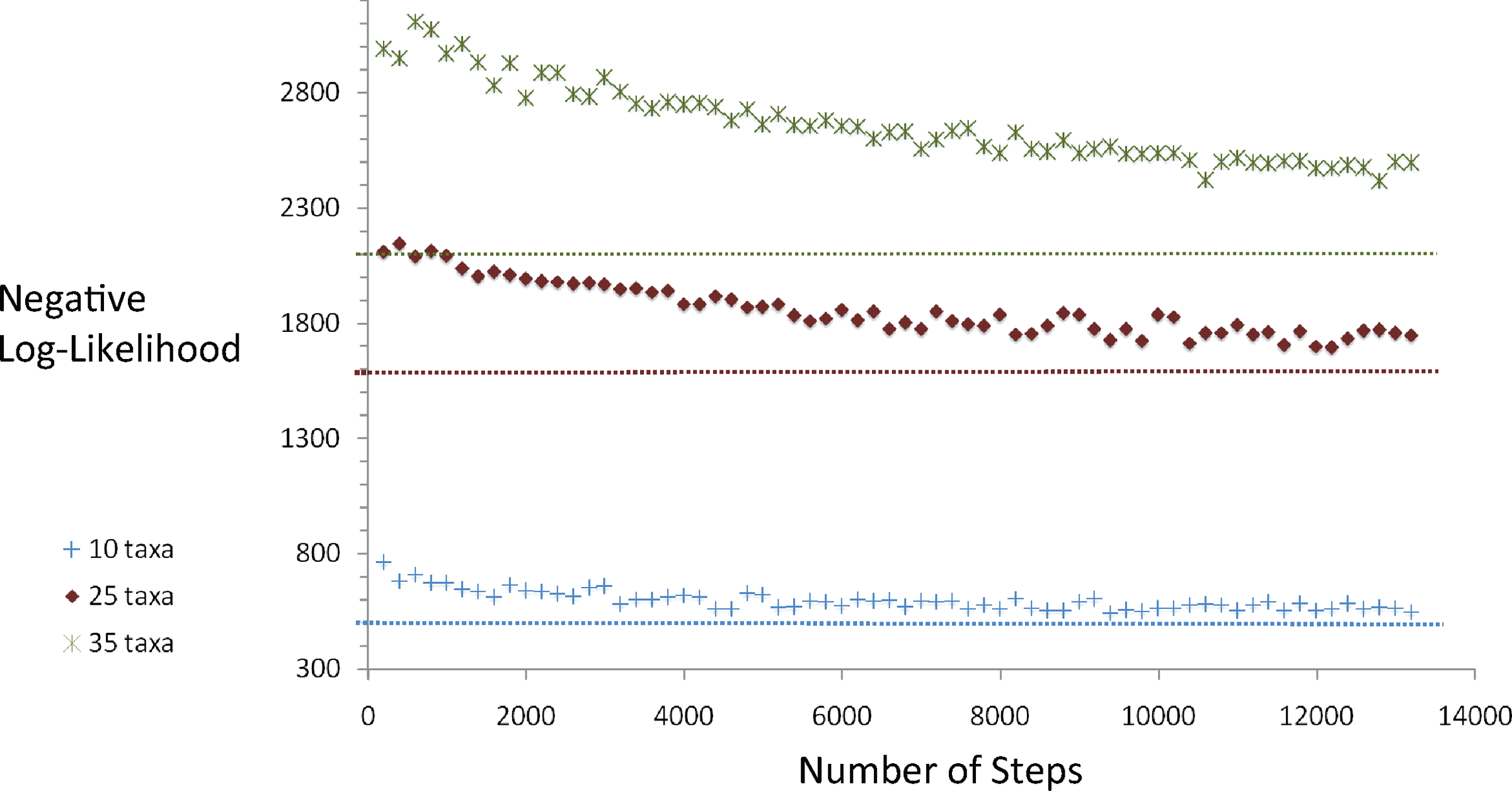
We first report results on experiments where we varied the number of taxa, keeping all other simulation and sampling parameters constant. In each case, data was simulated on trees with each edge probability fixed at 0.1, so, on average, one in ten characters mutated along each edge of the tree. For the Monte Carlo sampling step, we used three coupled chains maintained at temperatures (or β−1) = 1, 1.01 and 1.02. The temperatures were chosen heuristically (Huelsenbeck and Ronquist, 2001). After every 10 steps, two chains were picked at random and an attempt at swapping their states was made. These experiments were performed to assess the feasibility (both in run time performance and Markov chain convergence) of the proposed method.
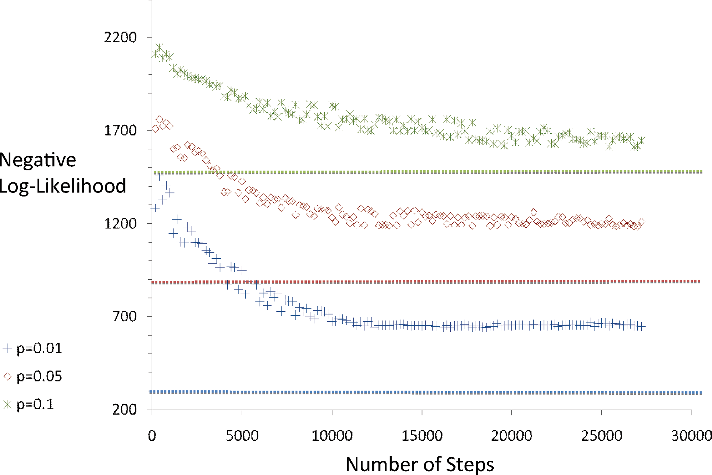
For the second set of experiments, we fixed the number of taxa to 25 and simulated data for edge probabilities values of 0.01, 0.05, and 0.1. These experiments were performed to estimate the variation in the uncertainty in inferring the true topology as well as the rate of convergence of the Markov chain.
6.2. Results
Figure 2 shows inferred likelihoods per Monte Carlo step for each tree. The plot reveals that the sampler relaxes to a high likelihood tree in each case. Further, the number of steps until the likelihood plateaus increases monotonically with the number of taxa, as expected. However, due to the low temperature and our use of the replica exchange heuristic in these empirical tests, we cannot assert with certainty that these chains are well-mixed. The dashed horizontal lines, representing the ancestral likelihood for the source tree, seem to indicate that each chain is quite probably close to equilibrium.
Inferred negative log-likelihood as a function of Monte Carlo step for trees of 10, 25, and 35 taxa.
Analysis of run times further shows the method to be very fast in practice despite the need for solving a hard optimization problem at each step. Table 1 shows mean run-times expressed in numbers of Monte Carlo steps solved per second. Run time does increase with numbers of taxa, but is still more than 1500 steps per minute for 35 taxa trees. The method is thus practical for tens of thousands of steps of Markov chain sampling on moderate problem sizes. For instance, each run presented in Figure 2 took less than 23 minutes.
Run Time and Mismatch between True and Sampled Tree Topologies for Three Input Sizes
No. of taxa
ILP steps per second
Average mismatch
10
728.21
0.39
25
70.45
2.38
35
29.26
2.58
Table 1 also shows the results of the uncertainty analysis. While the most likely ancestral tree is known to be statistically inconsistent in general, we see that the sampler is extremely efficient in identifying true bipartitions for these data sets.
The second set of experiments probes the ancestral likelihood landscape as we vary the mutation probabilities while keeping the number of taxa fixed at 25. Figure 3 shows the negative log-likelihood plots for three experiments with varying edge lengths. Once again we find that the sampled trajectories relax fairly rapidly to a high likelihood tree that is close to the likelihood of the source tree. Data sets with shorter branches (lower mutation probability) seem to relax faster, although we once again cannot assert that with certainty.
Inferred negative log-likelihood as a function of Monte Carlo step for trees with 25 taxa and varying edge probabilities.
Table 2 gives us additional insight into the likely dynamics of the Markov chain. As the mutation probabilities along tree edges increase, so does the accuracy of inferring the source tree. On the other hand, looking at Figure 3 seems to suggest that the sampler relaxes more rapidly for high edge probability data. This set of experiments thus tends to strongly suggest that near equilibrium, the ability of the sampler to estimate the source tree deteriorates as edge probabilities become small. This agrees with our intuition that given two speciation events, it should be relatively easier to infer the order in which they occur if the sequences at the two branch points are “well separated” (i.e., the branch length between the internal edges is large). At the same time, in the neighborhood of trees with long branches, the ancestral likelihood is comparably “flatter” (for the same reason that the peak of the likelihood curve in Lemma 2 is at the shortest branch). As a result, the Markov chain moves about the state space comparably faster (leading to a lower rejection ratio in Table 2), but at each new node the optimal tree does not differ much from the true tree. On the other hand, for extremely short branches, the most likely ancestral sequences are closely clustered together around a smaller region of the state space and Markov chain rarely ventures out of this central region (leading to a high rejection ratio). However, since most ancestral nodes have largely similar sequences for the low edge probability case, it is relatively more common to swap the order of bifurcation events connecting two ancestral nodes, leading to a higher mismatch between the average estimated topology and the source tree. For the 0.01 edge probability case, the source tree had numerous higher degree internal nodes (or edges with zero branch lengths) and that may be the likely cause for the mismatch. In phylogenetics, it is well known that near polytomies or very closely spaced bifurcation events are generally harder to reconstruct from fixed length sequences (Rokas and Carroll, 2006) and our experiments seem to suggest a similar effect on our ancestral likelihood sampler.
Rejection Ratio and Mismatch between True and Sampled Tree Topologies for Three Different Edge Probabilities for 25 Taxa Data Sets
Average edge probabilities
Average mismatch
Average rejection ratio
0.01
14.05
0.97
0.05
4.82
0.94
0.10
2.93
0.87
6.3. Discussion
Our experiments show that our method provides an efficient sampler over the ancestral likelihood model for relatively large numbers of taxa. Although the method involves solving a formally intractable problem at each step of Markov chain sampling, in practice it proves extremely fast for even moderately large data sets. Furthermore, our novel formulation allows us to examine aspects of the tree likelihood distribution inaccessible to standard samplers. Maximum ancestral likelihood has been known to be a statistically inconsistent estimator of the tree topology in general. Our experiments seem to indicate that the discrepancy between the topology of the average ancestral reconstruction and the source tree is small and robust to the number of leaves in the tree, except when the source tree has extremely short branch lengths.
7. Conclusion
We have developed a novel approach to phylogenetics designed to leverage methods for fast combinatorial optimization to efficiently sample over the space of phylogenetic trees under standard likelihood models. The method depends on an alternative formulation of phylogenetic likelihood to enable sampling over internal node states instead of tree topologies. The work establishes a new approach to performing efficient, accurate sampling over phylogenies and to establishing mixing time bounds for such sampling in practice. To demonstrate its theoretical value, we have established mixing time bounds for the important practical case of the CFN model. These bounds can be extended to some generalizations of that model and provide a new strategy for establishing provable bounds on more general likelihood models. We further demonstrate the practical efficiency and utility of the method through a study of uncertainty in topology inference across samples under a standard likelihood function. The ideas developed here for efficient optimization-based sampling may be applicable to many similar problems involving sampling over likelihoods of combinatorial objects.
Footnotes
Acknowledgments
This work was supported by U.S. National Science Foundation (grant 0612099 to N.M., G.B., R.R., and R.S.). Additionally, this work was supported by U.S. National Institutes of Health (grants 1R01CA140214 and 1R01AI076318 to R.S.).
Disclosure Statement
No competing financial interests exist.
References
1.
BubleyR., DyerM.1997. Path coupling: a technique for proving rapid mixing in Markov chains. Proc. 38th Annu. Symp. Found. Comput. Sci., 223–231.
2.
CavenderJ.A.1978. Taxonomy with confidence. Math. Biosci., 40:271–280.
3.
DiaconisP., HolmesS.P.2002. Random walks on trees and matchings. Electron. J. Probab., 7:6.
4.
FarrisJ.S.1973. A probability model for inferring evolutionary trees. Syst. Zool., 22:250–256.
HuelsenbeckJ.P., RonquistF.2001. MRBAYES: Bayesian inference of phylogeny. Bioinformatics, 17:754–755.
7.
LevinD.A., PeresY., WilmerE.A.2008. Markov Chains and Mixing Times. American Mathematical Society: Providence, RI.
8.
MisraN., SchwartzR.2008. Efficient stochastic sampling of first-passage time with applications to self-assembly simulation. J. Chem. Phys., 129:204109.
9.
MosselE., VigodaE.2005. Phylogenetic MCMC algorithms are misleading on mixtures of trees. Science, 309:2207–2209.
10.
NeymanJ.1971. Molecular studies of evolution: a source of novel statistical problems, 1–27. GuptaS.S., YackelJ.Statistical Decision Theory and Related Topics. Academic Press: New York.
11.
RokasA., CarrollS.B.2006. Bushes in the Tree of Life. PLoS Biol., 4:e352.
12.
StefankovicD., VigodaE.2007. Pitfalls of heterogeneous processes for phylogenetic reconstruction. Syst. Biol., 56:113–124.
13.
StefankovicD., VigodaE.2010. Fast convergence of MCMC algorithms for phylogenetic reconstruction with homogeneous data on closely related speciesAvailable at arXiv:1003.5964.