Computing Fragmentation Trees from Metabolite Multiple Mass Spectrometry Data

Maximum Colorful Subtree problem

Given a vertex-colored DAG G = (V, E) with colors \documentclass{aastex} \usepackage{amsbsy} \usepackage{amsfonts} \usepackage{amssymb} \usepackage{bm} \usepackage{mathrsfs} \usepackage{pifont} \usepackage{stmaryrd} \usepackage{textcomp} \usepackage{portland, xspace} \usepackage{amsmath, amsxtra} \pagestyle{empty} \DeclareMathSizes {10} {9} {7} {6} \begin{document} $${\cal C}$$\end{document} and weights \documentclass{aastex} \usepackage{amsbsy} \usepackage{amsfonts} \usepackage{amssymb} \usepackage{bm} \usepackage{mathrsfs} \usepackage{pifont} \usepackage{stmaryrd} \usepackage{textcomp} \usepackage{portland, xspace} \usepackage{amsmath, amsxtra} \pagestyle{empty} \DeclareMathSizes {10} {9} {7} {6} \begin{document} $$w:E \to {\mathbb R}$$\end{document} . Find the induced colorful subtree T = (V_T, E_T) of G of maximum weight \documentclass{aastex} \usepackage{amsbsy} \usepackage{amsfonts} \usepackage{amssymb} \usepackage{bm} \usepackage{mathrsfs} \usepackage{pifont} \usepackage{stmaryrd} \usepackage{textcomp} \usepackage{portland, xspace} \usepackage{amsmath, amsxtra} \pagestyle{empty} \DeclareMathSizes {10} {9} {7} {6} \begin{document} $$w ( T ) : = \sum \nolimits_{e \in E_T} w ( e )$$\end{document} .

We now modify this problem to take into account MS ⁿ data when constructing fragmentation trees. From the experimental data, we construct a DAG G = (V, E) together with a vertex coloring \documentclass{aastex} \usepackage{amsbsy} \usepackage{amsfonts} \usepackage{amssymb} \usepackage{bm} \usepackage{mathrsfs} \usepackage{pifont} \usepackage{stmaryrd} \usepackage{textcomp} \usepackage{portland, xspace} \usepackage{amsmath, amsxtra} \pagestyle{empty} \DeclareMathSizes {10} {9} {7} {6} \begin{document} $$c: V \rightarrow {\cal C}$$\end{document} , called fragmentation graph. Recall that the vertices of V correspond to potential molecular formulas of the fragments, colors \documentclass{aastex} \usepackage{amsbsy} \usepackage{amsfonts} \usepackage{amssymb} \usepackage{bm} \usepackage{mathrsfs} \usepackage{pifont} \usepackage{stmaryrd} \usepackage{textcomp} \usepackage{portland, xspace} \usepackage{amsmath, amsxtra} \pagestyle{empty} \DeclareMathSizes {10} {9} {7} {6} \begin{document} $${\cal C}$$\end{document} correspond to peaks in the mass spectra, and molecular formulas corresponding to the same peak mass have the same color. In contrast to the fragmentation graph where each edge indicates a direct succession, the MS ⁿ data does not only hint to direct but also to indirect successions. So, in the graph constructed from the MS ⁿ data we also have to score the transitive closure of the induced subtrees. The transitive closure G⁺ = (V, E⁺) of a DAG G = (V, E) contains the edge \documentclass{aastex} \usepackage{amsbsy} \usepackage{amsfonts} \usepackage{amssymb} \usepackage{bm} \usepackage{mathrsfs} \usepackage{pifont} \usepackage{stmaryrd} \usepackage{textcomp} \usepackage{portland, xspace} \usepackage{amsmath, amsxtra} \pagestyle{empty} \DeclareMathSizes {10} {9} {7} {6} \begin{document} $$( u , v ) \in E^ +$$\end{document} if and only if there is a directed path in G from u to v. In case G is a tree, the transitive closure can be computed in time O(|V|²) using Nuutila's algorithm (Nuutila, 1994). The MS ⁿ data gives additional information about the provenience of certain peaks/colors, but does not differentiate between different explanations of these peaks via molecular formulas, so we will score not edges but pairs of colors.

To score the closure, let \documentclass{aastex} \usepackage{amsbsy} \usepackage{amsfonts} \usepackage{amssymb} \usepackage{bm} \usepackage{mathrsfs} \usepackage{pifont} \usepackage{stmaryrd} \usepackage{textcomp} \usepackage{portland, xspace} \usepackage{amsmath, amsxtra} \pagestyle{empty} \DeclareMathSizes {10} {9} {7} {6} \begin{document} $$w^ + : {{\cal C}^2 \rightarrow {\mathbb R}}$$\end{document} be a weighting function for pairs of colors. We define the transitive weight of an induced tree T = (V_T, E_T) with transitive closure \documentclass{aastex} \usepackage{amsbsy} \usepackage{amsfonts} \usepackage{amssymb} \usepackage{bm} \usepackage{mathrsfs} \usepackage{pifont} \usepackage{stmaryrd} \usepackage{textcomp} \usepackage{portland, xspace} \usepackage{amsmath, amsxtra} \pagestyle{empty} \DeclareMathSizes {10} {9} {7} {6} \begin{document} $$T^ + = ( V_T , E_T^ + )$$\end{document} as: \documentclass{aastex} \usepackage{amsbsy} \usepackage{amsfonts} \usepackage{amssymb} \usepackage{bm} \usepackage{mathrsfs} \usepackage{pifont} \usepackage{stmaryrd} \usepackage{textcomp} \usepackage{portland, xspace} \usepackage{amsmath, amsxtra} \pagestyle{empty} \DeclareMathSizes {10} {9} {7} {6} \begin{document} \begin{align*}w^ + ( T ) : = \mathop\sum \limits_{ ( u , v ) \in E_T^ + } w^ + \left ( c ( u ) , c ( v ) \right ) \tag{1}\end{align*}\end{document}

Again, we limit our search to colorful trees, where each color is used at most once in the tree. Scoring the transitive closure of an induced colorful subtree, we reach the following problem definition:

Colorful Subtree Closure problem

Given a vertex-colored DAG G = (V, E) with colors \documentclass{aastex} \usepackage{amsbsy} \usepackage{amsfonts} \usepackage{amssymb} \usepackage{bm} \usepackage{mathrsfs} \usepackage{pifont} \usepackage{stmaryrd} \usepackage{textcomp} \usepackage{portland, xspace} \usepackage{amsmath, amsxtra} \pagestyle{empty} \DeclareMathSizes {10} {9} {7} {6} \begin{document} $${\cal C}$$\end{document} and transitive weights \documentclass{aastex} \usepackage{amsbsy} \usepackage{amsfonts} \usepackage{amssymb} \usepackage{bm} \usepackage{mathrsfs} \usepackage{pifont} \usepackage{stmaryrd} \usepackage{textcomp} \usepackage{portland, xspace} \usepackage{amsmath, amsxtra} \pagestyle{empty} \DeclareMathSizes {10} {9} {7} {6} \begin{document} $$w^ + : {\cal C}^2 \rightarrow {\mathbb R}$$\end{document} . Find the induced colorful subtree T of G of maximum weight w⁺(T).

We will see in the next section that this is again a computationally hard problem. But the problem we are interested in is even harder as it combines the two above problems:

Combined Colorful Subtree problem

Given a vertex-colored DAG G = (V, E) with colors \documentclass{aastex} \usepackage{amsbsy} \usepackage{amsfonts} \usepackage{amssymb} \usepackage{bm} \usepackage{mathrsfs} \usepackage{pifont} \usepackage{stmaryrd} \usepackage{textcomp} \usepackage{portland, xspace} \usepackage{amsmath, amsxtra} \pagestyle{empty} \DeclareMathSizes {10} {9} {7} {6} \begin{document} $${\cal C}$$\end{document} , edge weights \documentclass{aastex} \usepackage{amsbsy} \usepackage{amsfonts} \usepackage{amssymb} \usepackage{bm} \usepackage{mathrsfs} \usepackage{pifont} \usepackage{stmaryrd} \usepackage{textcomp} \usepackage{portland, xspace} \usepackage{amsmath, amsxtra} \pagestyle{empty} \DeclareMathSizes {10} {9} {7} {6} \begin{document} $$w:E \rightarrow {\mathbb R}$$\end{document} , and transitive weights \documentclass{aastex} \usepackage{amsbsy} \usepackage{amsfonts} \usepackage{amssymb} \usepackage{bm} \usepackage{mathrsfs} \usepackage{pifont} \usepackage{stmaryrd} \usepackage{textcomp} \usepackage{portland, xspace} \usepackage{amsmath, amsxtra} \pagestyle{empty} \DeclareMathSizes {10} {9} {7} {6} \begin{document} $$w^ + : {\cal C}^2 \rightarrow {\mathbb R}$$\end{document} . Find the induced colorful subtree T of G of maximum weight w*(T) = w(T) + w⁺(T).

3. Hardness Results

Fellows et al. (2007) and Böcker and Rasche (2008) independently showed that the Maximum Colorful Subtree problem is NP-hard. It turns out that the Colorful Subtree Closure problem is NP-hard even for unit weights:

Theorem 1

The Colorful Subtree Closure problem is NP-hard even if the input graph is a binary tree with unit weights w⁺ ≡ 1.

Proof

To prove NP-hardness we use a reduction from the NP-hard 3-Sat* problem (Berman et al., 2007):

3-SAT*

Given a Boolean expression in conjunctive normal form (CNF) consisting of a set of length three clauses, where each variable occurs at most three times in the clause set. Decide whether the expression is satisfiable.

Given an instance of 3-SAT* as a CNF formula \documentclass{aastex} \usepackage{amsbsy} \usepackage{amsfonts} \usepackage{amssymb} \usepackage{bm} \usepackage{mathrsfs} \usepackage{pifont} \usepackage{stmaryrd} \usepackage{textcomp} \usepackage{portland, xspace} \usepackage{amsmath, amsxtra} \pagestyle{empty} \DeclareMathSizes {10} {9} {7} {6} \begin{document} $$\Psi = c_1 \wedge \cdots \wedge c_m$$\end{document} over variables \documentclass{aastex} \usepackage{amsbsy} \usepackage{amsfonts} \usepackage{amssymb} \usepackage{bm} \usepackage{mathrsfs} \usepackage{pifont} \usepackage{stmaryrd} \usepackage{textcomp} \usepackage{portland, xspace} \usepackage{amsmath, amsxtra} \pagestyle{empty} \DeclareMathSizes {10} {9} {7} {6} \begin{document} $$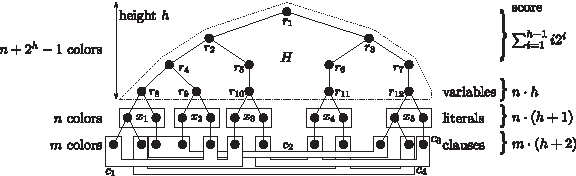x_1 , \cdots , x_n$$\end{document} we construct an instance of Colorful Subtree Closure. Since variables occurring only with one literal are trivial, we assume that the formula contains both literals of each variable. We first construct a colorful binary tree H with root vertex r and n leaves, that has height h : = ⌈log₂ n⌉ and is a perfect binary tree up to height h − 1. This tree uses p : = n + 2 ^h  − 1 colors, namely \documentclass{aastex} \usepackage{amsbsy} \usepackage{amsfonts} \usepackage{amssymb} \usepackage{bm} \usepackage{mathrsfs} \usepackage{pifont} \usepackage{stmaryrd} \usepackage{textcomp} \usepackage{portland, xspace} \usepackage{amsmath, amsxtra} \pagestyle{empty} \DeclareMathSizes {10} {9} {7} {6} \begin{document} $$r_{1} , \cdots, r_{p}$$\end{document} . To each leaf i, 1 ≤ i ≤ n, we connect two vertices using the same color x_i and representing the different truth assignments for x_i. One vertex in the color x_i represents x_i = true, the other one x_i = false. If a truth assignment to x_i satisfies clause c_j we connect a vertex colored c_j to the vertex in the color x_i, that corresponds to this truth assignment (Fig. 1). The resulting tree G possesses n + 2 ^h  − 1 + n + m colors, namely \documentclass{aastex} \usepackage{amsbsy} \usepackage{amsfonts} \usepackage{amssymb} \usepackage{bm} \usepackage{mathrsfs} \usepackage{pifont} \usepackage{stmaryrd} \usepackage{textcomp} \usepackage{portland, xspace} \usepackage{amsmath, amsxtra} \pagestyle{empty} \DeclareMathSizes {10} {9} {7} {6} \begin{document} $$r_{1} , \cdots, r_{p} , x_{1} , \cdots, x_{n} , c_{1} , \cdots, c_{m}$$\end{document} . The tree is binary, since each variable occurs in at most three clauses and we assumed that both literals are contained in the formula. Finally, we define unit weights w⁺ ≡ 1.

OPEN IN VIEWER

FIG. 1.

Proof of Theorem 1. Example for the construction of G for \documentclass{aastex} \usepackage{amsbsy} \usepackage{amsfonts} \usepackage{amssymb} \usepackage{bm} \usepackage{mathrsfs} \usepackage{pifont} \usepackage{stmaryrd} \usepackage{textcomp} \usepackage{portland, xspace} \usepackage{amsmath, amsxtra} \pagestyle{empty} \DeclareMathSizes {10} {9} {7} {6} \begin{document} $$\Phi = (x_1 \vee \overline {x_2} \vee x_3) \wedge (\overline{x_1} \vee x_2 \vee x_5 ) \wedge (\overline{x_3} \vee x_4 \vee \overline{x_5} ) \wedge (\overline{x_4} \vee x_5 \vee x_1).$$\end{document}

The resulting tree G has as many leaves as there are literals in Φ, hence the construction is polynomial. We claim that Φ is satisfiable if and only if the colorful subtree T of G with maximum transitive closure has score \documentclass{aastex} \usepackage{amsbsy} \usepackage{amsfonts} \usepackage{amssymb} \usepackage{bm} \usepackage{mathrsfs} \usepackage{pifont} \usepackage{stmaryrd} \usepackage{textcomp} \usepackage{portland, xspace} \usepackage{amsmath, amsxtra} \pagestyle{empty} \DeclareMathSizes {10} {9} {7} {6} \begin{document} $$\sum \nolimits _{i = 1}^{h - 1} i2^i + nh + n ( h + 1 ) + m ( h + 2 )$$\end{document} . To prove the forward direction, assume a truth assignment Φ that satisfies Φ. Define A ⊆ V(G) to be the subset of vertices in the colors x_i that correspond to the assignment Φ. Then, for every 1 ≤ j ≤ m there exists at least one vertex colored c_j in the neighborhood of A. Add an arbitrary representative of these vertices colored c_j to the set B ⊆ V(G). The union of the sets \documentclass{aastex} \usepackage{amsbsy} \usepackage{amsfonts} \usepackage{amssymb} \usepackage{bm} \usepackage{mathrsfs} \usepackage{pifont} \usepackage{stmaryrd} \usepackage{textcomp} \usepackage{portland, xspace} \usepackage{amsmath, amsxtra} \pagestyle{empty} \DeclareMathSizes {10} {9} {7} {6} \begin{document} $$A \cup B \cup \{ r_{1} , \cdots, r_{p} \} $$\end{document} forms a colorful subtree T of G with transitive closure that has score \documentclass{aastex} \usepackage{amsbsy} \usepackage{amsfonts} \usepackage{amssymb} \usepackage{bm} \usepackage{mathrsfs} \usepackage{pifont} \usepackage{stmaryrd} \usepackage{textcomp} \usepackage{portland, xspace} \usepackage{amsmath, amsxtra} \pagestyle{empty} \DeclareMathSizes {10} {9} {7} {6} \begin{document} $$\sum \nolimits _{i = 1}^{h - 1}i2^i + nh + n ( h + 1 ) + m ( h + 2 ) ,$$\end{document} as \documentclass{aastex} \usepackage{amsbsy} \usepackage{amsfonts} \usepackage{amssymb} \usepackage{bm} \usepackage{mathrsfs} \usepackage{pifont} \usepackage{stmaryrd} \usepackage{textcomp} \usepackage{portland, xspace} \usepackage{amsmath, amsxtra} \pagestyle{empty} \DeclareMathSizes {10} {9} {7} {6} \begin{document} $$\sum \nolimits _{i = 1}^{h - 1}i2^i$$\end{document} corresponds to the score of the perfect binary tree up to height h − 1, nh is the additional score from the leaves of H, n(h + 1) the additional score induced by the colors x_i and m(h + 2) the additional score induced by the colors c_j. No colorful subtree with higher score of the transitive closure can exist.

To prove the backward direction assume there is a colorful subtree T of G with maximum transitive closure that has score \documentclass{aastex} \usepackage{amsbsy} \usepackage{amsfonts} \usepackage{amssymb} \usepackage{bm} \usepackage{mathrsfs} \usepackage{pifont} \usepackage{stmaryrd} \usepackage{textcomp} \usepackage{portland, xspace} \usepackage{amsmath, amsxtra} \pagestyle{empty} \DeclareMathSizes {10} {9} {7} {6} \begin{document} $$\sum \nolimits _{i = 1}^{h - 1}i2^i + nh + n ( h + 1 ) + m ( h + 2 )$$\end{document} . Any optimal solution uses all colors from H, all colors x_i and all colors c_j. The truth assignment corresponding to the vertices of T colored x_i satisfies Φ, as for all 1 ≤ j ≤ m exactly one vertex colored c_j is connected to these vertices, otherwise T would not contain all colors.   ▪

We now turn to the inapproximability of the above problems. Dondi et al. (2011) show that the Maximum Motif problem, that is closely related to the Maximum Colorful Subtree problem, is APX-hard even if the input graph is a binary tree. In fact, Proposition 8 in Dondi et al. (2011) implies that the Maximum Colorful Subtree problem is APX-hard for such trees. We infer that there exists no Polynomial Time Approximation Scheme (PTAS) for the problem unless P = NP (Arora et al., 1998). In Proposition 10, Dondi et al. (2011) prove the even stronger result that there is no constant-factor approximation for Maximum Level Motif problem, unless P = NP.

Lemma 1

The Maximum Colorful Subtree problem is APX-hard even if the input graph is a binary tree with unit weights w ≡ 1.

Lemma 2

The Maximum Colorful Subtree problem has no constant-factor approximation unless P = NP, even if the input graph is a tree with unit weights w ≡ 1.

We now concentrate on the Colorful Subtree Closure problem. We note that for binary weights, the problem is APX-hard and has no constant-factor approximation. Next, we show that the problem is MAX SNP-hard even for unit weights. In both cases, we infer the non-existence of a PTAS unless P = NP (Arora et al., 1998).

Lemma 3

The Colorful Subtree Closure problem is APX-hard, even if the input graph is a binary tree with binary weights.

Lemma 4

The Colorful Subtree Closure problem has no constant-factor approximation unless P = NP, even if the input graph is a tree with binary weights.

Theorem 2

The Colorful Subtree Closure problem is MAX SNP-hard even if the input graph is a tree with unit weights w⁺ ≡ 1.

For the proofs of Lemmata 3 and 4, we reduce from Maximum Level Motif, by assigning weight one to all transitive edges from the root, and weight zero to all other edges. The construction used in the proof of Theorem 2 is very similar to that of Theorem 1. We defer the details to Appendix A.1.

We infer that the Combined Colorful Subtree problem is computationally hard and also hard to approximate, as it generalizes the above two problems. Note that the input graphs in our application are transitive graphs, whereas we assume trees in our hardness proofs. One might argue that the problem is actually simpler for transitive graphs; but for a given tree T = (V, E) with unit weights, its transitive closure G : = T⁺ can be complemented with a binary weighting w : E⁺ → {0, 1} such that w(e) = 1 if and only if \documentclass{aastex} \usepackage{amsbsy} \usepackage{amsfonts} \usepackage{amssymb} \usepackage{bm} \usepackage{mathrsfs} \usepackage{pifont} \usepackage{stmaryrd} \usepackage{textcomp} \usepackage{portland, xspace} \usepackage{amsmath, amsxtra} \pagestyle{empty} \DeclareMathSizes {10} {9} {7} {6} \begin{document} $$e \in E$$\end{document} . So, the Colorful Subtree Problem remains hard for transitive input graphs. Also note that the input graphs constructed from mass spectra, possess a topological sorting that respects colors. Again, one might argue that the problem is actually simpler for such graphs. It turns out that this is not the case, either: Dondi et al. (2011) show that the Maximum Motif problem is APX-hard even for leveled trees. All the trees constructed in our reductions are leveled, and all our results are also valid on leveled trees. Similar to above, leveled trees can be encoded in “color-sorted” graphs using binary weightings. Thus, the problems remain hard for graphs with this property.

The Maximum Colorful Subtree problem becomes tractable if the input graph is colorful and has non-negative edge weights: For undirected graphs, we can use Kruskal's or Prim's algorithm to compute a maximum spanning tree in polynomial time. For a DAG with a single source that has non-negative edge weights, the problem is even simpler: We can choose, for every vertex but the root, the incoming edge of maximum weight. For an arbitrary DAG with non-negative edge weights, consider separately the descent of each source. For general directed graphs with non-negative edge weights, the Chu-Liu/Edmonds Algorithm (Chu and Liu, 1965; Edmonds, 1967) will do the job. In contrast, the Colorful Subtree Closure problem remains hard, even for the most restricted case:

Theorem 3

The Colorful Subtree Closure problem is MAX SNP-hard even if the input graph is a colorful DAG with a single source and binary weights.

As we consider a colorful DAG, we can discard all colors and search for a subtree with maximum transitive closure. The transitive closure need not to be defined on colors, but can also be defined on vertices. So, each transitive edge has individual 0/1 weight. We defer the proof of Theorem 3 to Appendix A.2. This proof can be easily adapted to a DAG with maximal vertex degree three. So, the Colorful Subtree Closure problem is MAX SNP-hard even if the input graph is an in- and out-degree bounded, colorful DAG with a single source and binary weights.

Surprisingly, we can still find a swift and exact algorithm for the Colorful Subtree Closure problem, presented in the next section.

4. An Exact Algorithm for the Combined Colorful Subtree Problem

Several heuristics for the simpler Maximum Colorful Subtree problem have been evaluated both regarding quality of scores (Böcker and Rasche, 2008) and quality of fragmentation tree (Rasche et al., 2011). Results of using only the heuristics were of appalling quality, so we refrain from using only heuristics to solve the Combined Colorful Subtree problem. Furthermore, no constant-factor approximation can exist, unless P = NP. But despite the hardness of the problem, we will now present an exact algorithm with reasonable running time in applications. The algorithm is fixed-parameter tractable with respect to the number of colors k = |C|, and uses dynamic programming to find the optimum. Note that in application, we can choose k arbitrarily. Let n : = |V| and m : = |E| be the number of vertices and edges in the input graph G = (V, E), respectively.

Let W*(v, S) be the maximum score w*(T) of a colorful subtree with root v using colors S ⊆ C. Then W*(v, S) can be calculated as \documentclass{aastex} \usepackage{amsbsy} \usepackage{amsfonts} \usepackage{amssymb} \usepackage{bm} \usepackage{mathrsfs} \usepackage{pifont} \usepackage{stmaryrd} \usepackage{textcomp} \usepackage{portland, xspace} \usepackage{amsmath, amsxtra} \pagestyle{empty} \DeclareMathSizes {10} {9} {7} {6} \begin{document} \begin{align*}W^* ( v , S ) = \max \begin{cases} \max \limits_{u:c ( u ) \in S \setminus \{ c ( v ) \} } W^* ( u , S \setminus \{ c ( v ) \} ) + w ( v , u ) + \mathop\sum \limits_{c^{ \prime} \in S \setminus \{ c ( v ) \} }{w^ + \left ( c ( v ) , c^{ \prime} \right ) } \\ \\ \\ \max \limits_{{ ( S_1 , S_2 ) :S_1 \cap S_2 = \{ c ( v ) \} \atop S_1 \cup S_2 = S}} W^* ( v , S_1 ) + W^* ( v , S_2 ) \end{cases} \tag{2}\end{align*}\end{document}

where, obviously, we have to exclude the cases S₁ = {c(v)} and S₂ = {c(v)} from the computation of the second maximum. We initialize W*(v,{c(v)}) = 0, and set the weight of nonexistent edges to −∞. To prove the correctness of recurrence (2), we note that we only have to differentiate three cases: A subtree root v can have no children, one child, or two or more children. The case of no children, that is v is a leaf, is covered by the initialization. If v has one child u, we add the score of the tree rooted in u, the score of the new edge (v, u), and scores of all new transitive edges. This is done in the first line of the recurrence. If v has two or more children, we can “glue together” two trees rooted in v, where we arbitrarily distribute the children of v and the colors of S to the two trees.

We now analyze the running time of recurrence (2). Extending a tree by a single vertex takes O(2^km) time, as we can calculate the sum in constant time by going over the 2 ^k partitions in a reasonable order. Gluing together two trees, the k colors are partitioned into three groups: those not contained in S, elements of S₁, and elements of S₂. There are 3 ^k possibilities to perform this partition, so running time is O(3^kn). This results in a total running time of O(3^kn + 2^km). Running time can be improved to O*(2 ^k ) using subset convolutions and the Möbius transform (Björklund et al., 2007), but this is of theoretical interest only. In comparison to the algorithm presented in Böcker and Rasche (2008), the worst-case running time is not affected by scoring the transitive closure. The necessary space is O(2^kn). In our implementation, we only iterate over defined values in W*: An entry is not defined if there exists no subtree rooted in v using exactly the colors in S. This algorithm engineering technique does not improve worst-case running times and memory consumption, but greatly improves them in practice. To decrease memory consumption, we use hash maps instead of arrays.

Unfortunately, the above method is limited by its memory and time consumption. In application, exact calculations are limited to k′ ≤ k colors for some moderate k′, such as k′ = 15. These colors correspond to the k′ most intense peaks in the mass spectra, as these contribute most to our scoring. The remaining peaks are added in descending intensity order by a greedy heuristic: For each vertex v with an unassigned color, we try to attach v to every vertex u of the tree constructed so far, where some or all of the children of u in the tree may become children of v. We omit the technical details, and just note that our heuristic is inspired by Kruskal's algorithm for computing a maximum spanning tree.

5. Scoring

Particularly in fragmentation spectra, the charge of metabolites is mostly ± 1, so we may assume that m/z and mass are equal. Note that our calculations are not limited to a charge of one, though.

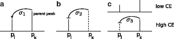
The transitive closure score w⁺ is defined using the MS ⁿ data. Recall that this score is defined for peaks or, equivalently, colors. In detail, we score three cases (Fig. 2):

• A spectrum with parent peak p_k and peak p_l indicates that the fragment corresponding to p_l has evolved from the fragment corresponding to p_k. To reward this, we increase the transitive score of the tree by σ₁ ≥ 0 if the fragment corresponding to p_k is a direct or indirect ancestor of the fragment corresponding to p_l (Fig. 2a).

• Given a spectrum that contains peak p_l but not peak p_k, and mass p_l < mass p_k. This indicates that the fragment corresponding to p_l has not evolved from the fragment corresponding to p_k. To penalize this, we add σ₂ ≤ 0 to the score if the fragment corresponding to p_k is a direct or indirect ancestor of the fragment corresponding to p_l (Fig. 2b).

• Given two spectra with different collision energies and two peaks p_k and p_l with mass p_l < mass p_k. If the spectrum with higher collision energy contains only p_k but the spectrum with lower collision energy contains both peaks, the fragment corresponding to p_l has probably not evolved from the fragment corresponding to p_k. This can be reasoned by contradiction: if the fragment corresponding to p_l had evolved from the fragment corresponding to p_k and this fragmentation process even happens with lower collision energy, it should also happen with higher collision energy. To penalize this case, we add σ₃ ≤ 0 to the score if the fragment corresponding to p_k is a direct or indirect ancestor of the fragment corresponding to p_l (Fig. 2c).

OPEN IN VIEWER

FIG. 2.

Scoring of the transitive closure referring to the three cases. A dashed peak is not occurring in the spectrum drawn but in another one (typically the MS² spectrum). A connection p_k → p_l indicates that p_l is a fragment of p_k while a connection p_k ⊣p_l indicates that peak p_l is unlikely to be a fragment of p_k.

In all cases, σ₁, σ₂, and σ₃ are not used to score edges of the fragmentation tree but instead, edges of the transitive closure of the tree. Two peaks are identified to correspond to the same fragment if their masses differ in less than 0.1 Da. For each fragment, only the peak with maximum intensity is taken into account for further calculations.

The scoring scheme of the fragmentation graph is the same as introduced in Böcker and Rasche (2008), taking the following properties into account: peak intensities, mass deviation between explanation and peak, chemical properties, collision energies and neutral losses. First, every peak is given a base score of b, b ≥ 0. To score the mass deviation we evaluate the logarithmized Gaussian probability density function with SD σ at the measuring error value. Further we use the density function of the normal distribution with mean 0.59 and SD 0.56 to score the hetero atom to carbon ratio of the decompositions. Due to the collision energies of the different spectra, some peaks cannot represent fragments of other peaks. A fragment appearing at lower collision energy than its predecessor is penalized with log(α), α ≪ 1. If there is no spectrum containing both, neither containing none of the peaks we add only a penalty of log(β), α < β < 1. Common neutral losses are rewarded with log(γ), γ > 1, while radical neutral losses are penalized by log(δ), δ < 1, and large neutral losses by \documentclass{aastex} \usepackage{amsbsy} \usepackage{amsfonts} \usepackage{amssymb} \usepackage{bm} \usepackage{mathrsfs} \usepackage{pifont} \usepackage{stmaryrd} \usepackage{textcomp} \usepackage{portland, xspace} \usepackage{amsmath, amsxtra} \pagestyle{empty} \DeclareMathSizes {10} {9} {7} {6} \begin{document} $$\log \Bigg( 1 - \frac { \hbox { mass ( neutral loss ) } } { \hbox { parent mass } } \Bigg)$$\end{document} . In addition to the scoring from Böcker and Rasche (2008), we use an extension that takes into account rare neutral losses: If a neutral loss from Table 1 occurs in a fragmentation step we penalize it by adding log(η), η ≪ 1. We also penalize neutral losses that contain only carbon or only nitrogen atoms by adding log(ε), ε ≪ 1. In contrast, radical losses from Table 2 are not penalized, since they sometimes occur in fragmentation reactions.

OPEN IN VIEWER

Table 1.

Rare Neutral Losses

NL name	NL formula
H2	Molecular hydrogen
C2O	Dicarbon oxide
C4O	Tetracarbon oxide
C3H2	Unsaturated cyclopropane
C5H2	Unsaturated cyclopentane
C7H2	Unsaturated cycloheptane

The rare neutral losses (NL) used in our calculations. If an entry from this table occurs in a fragmentation step, the score of this step is significantly decreased.

OPEN IN VIEWER

Table 2.

Common Radical Losses

RL name	RL formula
H	Hydrogen radical
O	Oxygen radical
OH	Hydroxyl radical
CH3	Methyl radical
CH3O	Methoxy radical
C3H7	Propyl radical
C4H9	Butyl radical
C6H5O	Phenoxy radical

The common radical losses (RL) used in our calculations. Radical losses are penalized, unless they occur in this table.

6. Results

To evaluate our work, we implemented the algorithm in Java 1.6. As test data we used 185 mass spectra of 45 compounds, mostly representing plant secondary metabolites. The 185 mass spectra are composed of 45 MS² spectra, 128 MS³ spectra and twelve MS⁴ spectra (unpublished). All spectra were measured on a Thermo Scientific Orbitrap XL instrument. They were acquired under operator control with the 7500 resolution settings. The samples were introduced using a built-in infusion pump. Activation time was set at 30 ms with the activation parameter q = 0.25 and an isolation window of 1.5 mass units was used. Peak picking was performed using the Xcalibur software supplied with the instrument. The data set was analyzed with the following options: For decomposing peak masses we use a relative error of 20 ppm and the standard alphabet containing carbon (C), hydrogen (H), nitrogen (N), oxygen (O), phosphorus (P), and sulfur (S). For the construction of the fragmentation graph, we use the collision energy scoring parameters α = 0.1, β = 0.8, the neutral loss scoring parameters γ = 10, δ = 10⁻³, ε = 10⁻⁴, η = 10⁻³, the intensity scoring parameter λ = 0.1, the base score b = 0 and the standard deviation of the mass error σ = 20/3 as described in Böcker and Rasche (2008) and Rasche et al., (2011). We can identify the molecular formulas of the compounds from isotope pattern analysis and by calculating the fragmentation trees for all candidate molecular formulas (Rasche et al., 2011). In this article, we assume that this task has been solved beforehand, and that all molecular formulas are known.

Comparing trees. We evaluate the impact of using MS ⁿ instead of MS² data, as well as the influence of scoring parameters σ₁, σ₂, σ₃ from Section 5, using pairwise tree comparison. In each fragmentation tree, vertices are implicitly labeled by molecular formulas of the corresponding fragments. We limit our comparison to those fragments that appear in both trees, and discard orphan fragments. We distinguish four cases:

• A fragment is identically placed, if its parent fragments are identical in both trees.

• A fragment is pulled up, if its parent fragment in the second tree is one of its predecessors in the first tree (and the fragment is not identically placed).

• A fragment is pulled down, if its parent fragment in the first tree is one of its predecessors in the second tree (and the fragment is not identically placed).

• A fragment is regrafted, if it is not identically placed, pulled up or pulled down.

Interchanging first tree and second tree, the identically placed and regrafted fragments are the same, while the pulled up fragments become pulled down and vice versa.

The obvious way to evaluate our method would be to compare our results against some gold standard. Unfortunately, such gold standard is not available for our study. Rasche et al. (2011) have evaluated the method from Böcker and Rasche (2008) by expert annotation of MS² fragmentation trees for a subset of the compounds used in this paper. Unfortunately, the input data (that is, fragments observed in the MS² and MS ⁿ mode of the instrument) differ strongly. Hence, a comparison against these expert-annotated fragmentation trees is impossible.

As mentioned in Section 4, the exact algorithm is memory and time consuming. So, we use the exact algorithm for only the k′ most intense peaks, and attach the remaining peaks using a greedy heuristic. We find that decreasing k′ from 20 to 15, has a comparatively small effect on the computed fragmentation trees: 97.1% of the fragments were identically placed, 0.4% were pulled up, 0.6% were pulled down, and only 1.9% were regrafted. On the other hand, average running time per compound was decreased from 30.8 min to 3.97 s. In the remainder of this section, we set k′ = 15 and use only the 15 most intensive peaks for exact computations. Choosing a moderate k′ = 15 has a much stronger effect here, than it was observed for the Maximum Colorful Subtree problem (Böcker and Rasche 2008), where constructed fragmentation trees were practically identical for k′ = 15 and k′ = 20. We attribute this to the transitive scoring, which appears to be harder to grasp by the heuristic.

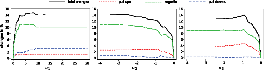
To show the effect of evaluating MS ⁿ data, we individually varied the three score parameters, and compared the resulting trees to the trees constructed without scoring the transitive closure (Fig. 3). As σ₁ increases, the fraction of changes in the trees (pull ups, pull downs and regrafts) converges to about 14%. A similar behavior is observed as σ₂,σ₃ are decreased. The main difference between the bonus score σ₁ and the penalty scores σ₂ and σ₃ is that increasing σ₁ results in more pull downs than pull ups, while decreasing penalty scores σ₂, σ₃ produces more pull ups than pull downs. This can be explained as follows: Reward scores can rather be realized if fragments are inserted deep, that is, far from the root. In contrast, negative penalty scores are avoided if the fragments are inserted “shallow”, that is, close to the root. So, σ₁ ≪ 0 tends to deepen the trees, whereas σ₂,σ₃ ≪ 0 tends to broaden the trees.

OPEN IN VIEWER

FIG. 3.

Result of individually varying the scoring parameters. Percentage of pull ups, pull downs, regrafted fragments, and total changed fragments when varying score parameters σ₁, σ₂, and σ₃. (Left) Varying σ₁ with σ₂ = 0 and σ₃ = 0 fixed. (Middle) Varying σ₂ with σ₁ = 0 and σ₃ = 0 fixed. (Right) Varying σ₃ with σ₁ = 0 and σ₂ = 0 fixed.

Based on the above analysis, we decided to use the following parameter values: k′ = 15, σ₁ = 3, σ₂ =−0.5, and σ₃ = −0.5. We choose a large σ₁ as the underlying MS ⁿ observation is a clear signal that some fragment should be placed as a successor of another fragment. In comparison, the MS ⁿ reasoning behind σ ₂ and σ₃ is somewhat weaker, so we choose smaller absolute values for these parameters that less influence the trees. The crucial comparison is now between the fragmentation trees computed without scoring the transitive closure and the fragmentation trees computed with the above scores. As we have only one MS² spectrum per compound and one spectrum contains too few peaks to calculate a reasonable tree, we transform the MS ⁿ data to “pseudo-MS²” data by merging all fragmentation spectra of a compound into one. This simulates MS² spectra with different collision energies. By merging all spectra into one, we loose all information about dependencies between peaks/colors. This is implicitly achieved by setting σ₁,σ₂,σ₃ = 0. Between these trees 76.21% of the fragments are identically connected, 4.90% are pull ups, 1.79% pull downs and 17.11% regrafted fragments. Hence, almost one quarter of all fragments are changed due to the information from MS ⁿ data.

We cannot evaluate whether these changed neutral losses are true or false and, hence, whether MS ⁿ fragmentation trees are truly better than the MS² trees. But we will now show two examples where the MS ⁿ trees agree well with the observed MS ⁿ data.

For the first example, we consider the fragmentation trees of phenylalanine, with and without scoring the transitive closure (Fig. 4). The two fragmentation trees are almost identical, with the single exception of fragment C₇H₉ at 93.1 Da: This fragment is connected to C₉H₉O₂ at 149.0 Da in the MS² tree, and to C₈H₁₀N at 120.1 Da in the MS ⁿ tree. In the MS² interpretation, the neutral loss C₂O₂ is explained as two common neutral losses CO and, hence, it is preferred over the neutral loss CHN (hydrogen cyanide). Using MS ⁿ data, we can resolve this: the peak at 93.1 Da does occur in the MS³ spectrum with parent peak at 120.1 Da, therefore C₇H₉ at 93.1 Da probably resulted (directly or indirectly) as a fragment of C₈H₁₀N at 120.1 Da. This is rewarded by our algorithm, adding σ₁ = +3 to the score of the modified tree. The fact that the peak at 107.0 Da is missing in the MS³ spectrum with parent peak at 120.1 Da, does not change the score: In the MS² analysis, fragment C₇H₇O cannot be a successor of C₈H₁₀N at 120.1 Da, nor are 91.1 Da, 93.1 Da, or 103.1 Da assumed to be its successor.

OPEN IN VIEWER

FIG. 4.

Fragmentation trees and mass spectra of phenylalanine. (Left) Fragmentation trees of phenylalanine. Solid edges are neutral losses present in both trees, the red dotted (green dashed) edge is present in the MS² (or MS ⁿ ) tree only, respectively. (Right) MS² spectrum of the parent peak (top) and MS³ spectrum of the 120.1 Da fragment (bottom). Dashed peaks are not contained in the particular spectrum.

Another example where the MS ⁿ tree agrees well with the observed MS ⁿ data is tryptophan. Figure 5 shows the fragmentation trees of tryptophan, with and without scoring the transitive closure and the corresponding spectra. The two fragmentation trees differ in three fragments: C₉H₈NO at 146.1 Da, C₆H₆N at 92.0 Da and C₄H₂NO at 80.0 Da. The fragment C₉H₈NO is pulled down in the MS ⁿ tree and connected to C₁₁H₁₀NO₂ at 188.1 Da. This is supported by the the MS³ spectrum with parent peak at 188.1 Da: it contains the fragment C₉H₈NO at 146.1 Da as well as its child fragment C₈H₈N at 118.1 Da. So, the transitive closure score is increased by 2σ₁ = 6. Fragment C₆H₆N at 92.0 Da is no longer present in the MS ⁿ tree. This change is supported by the MS³ and the MS⁴ spectra: if the neutral loss C₃H₂O dissociates from C₉H₈NO even with 15 eV collision energy in the MS² spectrum, this should also happen in the other two spectra with collision energy ≥ 15 eV. As this is not the case, the transitive closure score would decrease by 2σ₃ = −1 if C₆H₆N at 92.0 Da were connected to C₉H₈NO at 146.1 Da. As the score of edge C₃H₂O is smaller than 1, omitting the fragment C₆H₆N at 92.0 Da leads to a tree with higher score. In contrast, C₄H₂NO at 80.0 Da is not part of the MS² tree, but in the MS ⁿ tree it is child of C₉H₈NO at 146.1 Da. All incoming edges of C₄H₂NO must have negative score, otherwise the fragment would be part of the MS² tree. But the MS³ spectrum with parent peak at 146.1 Da contains a peak at 80.0 Da and so the score of the transitive closure is increased by σ₁ = 3 for the corresponding edge. This compensates the negative score of edge C₅H₆. Therefore, the fragment C₄H₂NO at 80.0 Da is added to the MS ⁿ tree.

OPEN IN VIEWER

FIG. 5.

Fragmentation trees and mass spectra of tryptophan. (Left) Fragmentation trees of tryptophan. Solid edges are neutral losses present in both trees, red dotted (green dashed) edges and nodes are present in the MS² (or MS ⁿ ) tree only, respectively. (Right) MS² spectrum of the parent peak (top), MS³ spectrum of the 188.1 Da fragment (middle) and MS⁴ spectrum of the 146.1 Da fragment (bottom). Dashed peaks are not contained in the particular spectrum. Only those scores responsible for the differences between the trees are shown in the spectra.

We have noted above, that MS² trees computed from our data, differ strongly from those computed from MS² data of Rasche et al. (2011), as the input data is different: The “pseudo-MS²” data used here, was in fact a union of MS² and MS ⁿ spectra. To this end, we also compare “pseudo-MS²” fragmentation trees computed for this study, with MS² trees computed from MS² data in Rasche et al. (2011): On average, only 72.33% of the fragments were identically placed, 6.05% were pulled up, 6.05% were pulled down, and 15.58% were regrafted.

As shown in Section 3, the theoretical worst case running time of our algorithm is identical with that of the Maximum Colorful Subtree algorithm in Böcker and Rasche (2008). We investigated whether this also holds in application. Running times were measured on an Intel Core 2 Duo, 2.4 GHz with 4 GB memory, with parameter k′ = 15. We split up our running time analysis into three parts: decomposition of peak masses, construction of the fragmentation graph plus calculation of the transitive closure, and the actual algorithm for finding a maximum colorful subtree. Maximum and average running times are shown in Table 3. Average running time for the graph construction is sixfold increased, but this contributes only negligible to the total running time. We find that total running times of the algorithm, with and without using MS ⁿ data, are practically identical: Average running time is about 3.8 s, and the maximal running time for one compound is 17.6 s.

OPEN IN VIEWER

Table 3.

Running Times

	Decomposition		Graph construction		Tree finding		Total
	Max	Average	Max	Average	Max	Average	Max	Average
MS2	14.90	1.37	0.17	0.01	5.29	2.38	17.32	3.76
MS n	14.91	1.37	0.19	0.07	5.12	2.40	17.58	3.84
Difference	+0.01	±0.00	+0.02	+0.06	−0.17	+0.02	+0.25	+0.08

Running time in seconds: Comparison of running times with (MS ⁿ ) and without (MS²) scoring transitive edges.

7. Conclusion

In this article, we have presented a framework for computing metabolite fragmentation trees using MS ⁿ data. Our fragmentation model results in the Combined Colorful Subtree problem, a conjunction of the Maximum Colorful Subtree problem and the Colorful Subtree Closure problem. Both problems are NP-hard, and no PTAS can exist for either problem. The latter problem remains MAX SNP-hard even if the input graph is colorful.

We have presented an exact dynamic programming algorithm for the Combined Colorful Subtree problem, showing that the problem is fixed-parameter tractable with respect to the parameter “number of colors.” We have introduced a scoring scheme based on the dependencies between the different fragmentation steps. To reduce memory and time requirements, we limit exact computations to the k′ ≤ k most intense peaks in the spectrum. Although the Combined Colorful Subtree problem is computationally hard, the resulting algorithm is fast in practice.

For our application, the score of the transitive closure \documentclass{aastex} \usepackage{amsbsy} \usepackage{amsfonts} \usepackage{amssymb} \usepackage{bm} \usepackage{mathrsfs} \usepackage{pifont} \usepackage{stmaryrd} \usepackage{textcomp} \usepackage{portland, xspace} \usepackage{amsmath, amsxtra} \pagestyle{empty} \DeclareMathSizes {10} {9} {7} {6} \begin{document} $$w^ + : {\cal C}^2 \rightarrow {\mathbb R}$$\end{document} is defined on pairs of colors. From the theoretical standpoint, one can modify the problem such that the score \documentclass{aastex} \usepackage{amsbsy} \usepackage{amsfonts} \usepackage{amssymb} \usepackage{bm} \usepackage{mathrsfs} \usepackage{pifont} \usepackage{stmaryrd} \usepackage{textcomp} \usepackage{portland, xspace} \usepackage{amsmath, amsxtra} \pagestyle{empty} \DeclareMathSizes {10} {9} {7} {6} \begin{document} $$w^ + : E^ + \rightarrow {\mathbb R}$$\end{document} is defined on edges of the transitive closure of the fragmentation graph G = (V, E). In this case, our algorithm from Section 4 cannot be used, and it remains an open problem whether this modified version of the Colorful Subtree Closure problem is fixed-parameter tractable with respect to the number of colors. Clearly, the problem is in FPT for unit weights.

We have seen that using additional information from MS ⁿ data does change the computed fragmentation trees. In our experiments, one quarter of fragments were differently inserted when including MS ⁿ information. As our scoring scheme is “chemically reasonable,” we argue that the trees are actually improved using MS ⁿ data. Unfortunately, MS ⁿ is less suited for high-throughput measurements, as individual measurements are more time-consuming. We suggest that, whenever experimentally possible, MS ⁿ should be used to calculate fragmentation trees, as it provides additional information. On the other hand, for about three quarters of the fragments, trees remain identical between MS² and MS ⁿ . Thus, calculating fragmentation trees from MS² data extracts valuable information concealed in these spectra and results in largely reasonable trees.

In the future, we want to increase the speed and decrease the memory consumption of our exact algorithm. Also, we want to use MS ⁿ fragmentation trees to fine-tune the scoring parameters for computing MS² fragmentation trees. The next step of the analysis pipeline is a method for automated comparison of fragmentation trees.

8. Appendix

A.1. Proof of Theorem 2 and Lemmata 3 and 4

Proof

First, we focus on Lemmata 3 and 4: In the proofs for Lemma 4, and Propositions 8, 9, and 10 from Dondi et al. (2011), constructed input trees are leveled, meaning that two different vertices can have the same color only if they have the same distance from the root. We attach an additional root r₊ to the original root r, connected by an edge (r₊, r). All vertices v keep their color c(v), and the additional root r₊ gets a unique color. We define transitive weights \documentclass{aastex} \usepackage{amsbsy} \usepackage{amsfonts} \usepackage{amssymb} \usepackage{bm} \usepackage{mathrsfs} \usepackage{pifont} \usepackage{stmaryrd} \usepackage{textcomp} \usepackage{portland, xspace} \usepackage{amsmath, amsxtra} \pagestyle{empty} \DeclareMathSizes {10} {9} {7} {6} \begin{document} \begin{align*}w^ + (c_1 , c_2) : = \begin{cases} {1 \quad {\rm if}\ {c_1} = c (r_ +)} , \\ {0 \quad {\rm otherwise.}} \end{cases}\end{align*}\end{document}

As the input tree T is leveled, finding a colorful subtree of T with n vertices is equivalent to finding a colorful subtree T′ of T with w⁺(T′) ≥ n. Lemma 4 in Dondi et al. (2011) ensures that the root of T is part of T′. Lemmata 3 and 4 now follow from Propositions 8, 9, and 10 in Dondi et al. (2011). Note that the root r also has a unique color; adding the root r₊ was done solely to get an additional +1 in the score of the tree.

Now, let us focus on the proof of Theorem 2. The MAX SNP-hardness concept was introduced by Papadimitriou and Yannakakis (1991). Let Π and Π′ be two optimization problems. We say that Π L-reduces to Π′ if there are two polynomial-time algorithms f, g and constants α,β > 0, such that for every instance I of Π:

1. Algorithm f produces an instance I′ = f (I) of Π′, such that the optima of I and I′, OPT(I) and OPT(I′), respectively, satisfy OPT(I′) ≤ α ·OPT(I).

2. Given any solution of I′ with cost c′, algorithm g produces a solution of I with cost c, such that |c − OPT(I)| ≤ β · |c′ − OPT(I′)|.

To prove MAX SNP-hardness of Colorful Subtree Closure, we L-reduce from Max-3Sat*, which is MAX SNP-hard (Papadimitriou and Yannakakis, 1991).

Max-3Sat*

Given a Boolean expression in conjunctive normal form (CNF) consisting of a set of length three clauses, where each variable occurs at most three times in the clause set. Find an assignment of the variables that satisfies as many clauses as possible.

Given a Max-3Sat* instance as a CNF formula \documentclass{aastex} \usepackage{amsbsy} \usepackage{amsfonts} \usepackage{amssymb} \usepackage{bm} \usepackage{mathrsfs} \usepackage{pifont} \usepackage{stmaryrd} \usepackage{textcomp} \usepackage{portland, xspace} \usepackage{amsmath, amsxtra} \pagestyle{empty} \DeclareMathSizes {10} {9} {7} {6} \begin{document} $$\Psi = c_{1} \wedge \cdots \wedge c_{m}$$\end{document} over variables \documentclass{aastex} \usepackage{amsbsy} \usepackage{amsfonts} \usepackage{amssymb} \usepackage{bm} \usepackage{mathrsfs} \usepackage{pifont} \usepackage{stmaryrd} \usepackage{textcomp} \usepackage{portland, xspace} \usepackage{amsmath, amsxtra} \pagestyle{empty} \DeclareMathSizes {10} {9} {7} {6} \begin{document} $$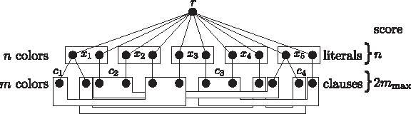x_{1} , \cdots , x_{n}$$\end{document} we construct an instance of Colorful Subtree Closure. Since variables occurring only with one literal are trivial, we assume that the formula contains both literals of each variable. We first construct a tree G with root vertex colored with r. We connect 2n children to it and assign every color x_i to exact two of them. The two vertices with color x_i represent both truth assignments of x_i. If a truth assignment to x_i satisfies clause c_j we connect a vertex colored c_j to the vertex x_i, that corresponds to this truth assignment. The resulting tree possesses n + m + 1 distinct colors, namely \documentclass{aastex} \usepackage{amsbsy} \usepackage{amsfonts} \usepackage{amssymb} \usepackage{bm} \usepackage{mathrsfs} \usepackage{pifont} \usepackage{stmaryrd} \usepackage{textcomp} \usepackage{portland, xspace} \usepackage{amsmath, amsxtra} \pagestyle{empty} \DeclareMathSizes {10} {9} {7} {6} \begin{document} $$r , x_1 , \cdots , x_n , c_1 , \cdots , c_m$$\end{document} . Finally, we define unit weights w⁺ ≡ 1 (Fig. 6).

OPEN IN VIEWER

FIG. 6.

Proof of Theorem 2. Example for the construction of G for \documentclass{aastex} \usepackage{amsbsy} \usepackage{amsfonts} \usepackage{amssymb} \usepackage{bm} \usepackage{mathrsfs} \usepackage{pifont} \usepackage{stmaryrd} \usepackage{textcomp} \usepackage{portland, xspace} \usepackage{amsmath, amsxtra} \pagestyle{empty} \DeclareMathSizes {10} {9} {7} {6} \begin{document} $$\Phi = ( x_1 \vee \overline{x_2} \vee x_3 ) \wedge (\overline{x_1} \vee x_2 \vee x_5 )\wedge ( \overline{x_3} \vee x_4 \vee \overline{x_5} ) \wedge ( \overline{x_4} \vee x_5 \vee x_1 )$$\end{document} .

The resulting tree has as many leaves as there are literals in Φ; hence, the construction is polynomial. From a solution of the Max-3Sat* instance that satisfies m_max clauses, we can construct a solution of the Colorful Subtree Closure instance with score 2m_max + n using n + m_max colors, and vice versa. To prove the forward direction, assume a truth assignment Φ satisfying m_max clauses from Φ. Define A ⊆ V (G) to be the subset of the vertices in the colors x_i that correspond to the assignment Φ. Then, for m_max colors c_j from \documentclass{aastex} \usepackage{amsbsy} \usepackage{amsfonts} \usepackage{amssymb} \usepackage{bm} \usepackage{mathrsfs} \usepackage{pifont} \usepackage{stmaryrd} \usepackage{textcomp} \usepackage{portland, xspace} \usepackage{amsmath, amsxtra} \pagestyle{empty} \DeclareMathSizes {10} {9} {7} {6} \begin{document} $$c_1 , \cdots , c_m$$\end{document} there exists at least one vertex of this color in the neighborhood of A. Add an arbitrary representative of these vertices colored c_j to the set B ⊆ V (G). The union of the sets \documentclass{aastex} \usepackage{amsbsy} \usepackage{amsfonts} \usepackage{amssymb} \usepackage{bm} \usepackage{mathrsfs} \usepackage{pifont} \usepackage{stmaryrd} \usepackage{textcomp} \usepackage{portland, xspace} \usepackage{amsmath, amsxtra} \pagestyle{empty} \DeclareMathSizes {10} {9} {7} {6} \begin{document} $$A \cup B \cup \{ r_{1} , \cdots , r_{p} \} $$\end{document} forms a colorful subtree T of G with maximum transitive closure that has score 2m_max + n, n from the variables and 2m_max from the fulfilled clauses. No colorful subtree with higher score of the transitive closure can exist.

To prove the backward direction, assume that there is a colorful subtree T from G with maximum transitive closure with score 2m_max + n. Any optimal solution uses all colors x_i and m_max colors c_j. Therefore, the truth assignment corresponding to the vertices of T colored x_i satisfies as many clauses from Φ as possible, as for all m_max colors c_j at least one vertex colored c_j is connected to these vertices, otherwise T would not contain all colors.

Now we show that our reduction is a L-reduction. Let OPT(CSC) denote the score of the optimal solution of the Colorful Subtree Closure instance, and OPT(M3S) denote the number of satisfied clauses in the optimal solution of the Max-3Sat* instance. Since the maximum score of the Colorful Subtree Closure instance is at most 2m + n and the number of variables n is at most 3m, we get OPT(CSC) ≤ 2m + n ≤ 5m. Since at least half of the clauses of the Max-3Sat* instance can be satisfied, we have OPT(M3S) ≥ m/2. Thus, OPT(CSC) ≤ α · OPT(M3S) holds for α : = 10.

Since |c − OPT(X)| = OPT(X) − c for a maximization problem X, we have to show that OPT(M3S) − c ≤ β · (OPT(CSC) − c′). We set β : = 1, then from c′ = c + m_max + n and OPT(CSC) = OPT(M3S)+ m_max + n we infer \documentclass{aastex} \usepackage{amsbsy} \usepackage{amsfonts} \usepackage{amssymb} \usepackage{bm} \usepackage{mathrsfs} \usepackage{pifont} \usepackage{stmaryrd} \usepackage{textcomp} \usepackage{portland, xspace} \usepackage{amsmath, amsxtra} \pagestyle{empty} \DeclareMathSizes {10} {9} {7} {6} \begin{document} \begin{align*}\beta \cdot ( OPT ( CSC ) - c^\prime ) = OPT ( CSC ) - c^\prime = OPT ( M3S ) + m_{\rm max} + n - ( c + m_{\rm max} + n ) = OPT ( M3S ) - c.\end{align*}\end{document}

So, the Colorful Subtree Closure problem is MAX SNP-hard, even for unit weights.   ▪

A.2. Proof of Theorem 3

Proof

Given a Max-3Sat* instance as a CNF formula \documentclass{aastex} \usepackage{amsbsy} \usepackage{amsfonts} \usepackage{amssymb} \usepackage{bm} \usepackage{mathrsfs} \usepackage{pifont} \usepackage{stmaryrd} \usepackage{textcomp} \usepackage{portland, xspace} \usepackage{amsmath, amsxtra} \pagestyle{empty} \DeclareMathSizes {10} {9} {7} {6} \begin{document} $$\Psi = c_{1} \land \cdots \land c_{m}$$\end{document} over variables \documentclass{aastex} \usepackage{amsbsy} \usepackage{amsfonts} \usepackage{amssymb} \usepackage{bm} \usepackage{mathrsfs} \usepackage{pifont} \usepackage{stmaryrd} \usepackage{textcomp} \usepackage{portland, xspace} \usepackage{amsmath, amsxtra} \pagestyle{empty} \DeclareMathSizes {10} {9} {7} {6} \begin{document} $$x_{1} , \cdots , x_{n}$$\end{document} we construct an instance of Colorful Subtree Closure where each color corresponds to one vertex. That means the graph is already colorful. We first construct a graph G with root vertex r. We connect 2n children to it, representing positive \documentclass{aastex} \usepackage{amsbsy} \usepackage{amsfonts} \usepackage{amssymb} \usepackage{bm} \usepackage{mathrsfs} \usepackage{pifont} \usepackage{stmaryrd} \usepackage{textcomp} \usepackage{portland, xspace} \usepackage{amsmath, amsxtra} \pagestyle{empty} \DeclareMathSizes {10} {9} {7} {6} \begin{document} $$( pl_{1} , \cdots , pl_{n} )$$\end{document} and negative literals \documentclass{aastex} \usepackage{amsbsy} \usepackage{amsfonts} \usepackage{amssymb} \usepackage{bm} \usepackage{mathrsfs} \usepackage{pifont} \usepackage{stmaryrd} \usepackage{textcomp} \usepackage{portland, xspace} \usepackage{amsmath, amsxtra} \pagestyle{empty} \DeclareMathSizes {10} {9} {7} {6} \begin{document} $$( nl_{1} , \cdots , nl_{n} )$$\end{document} of the variables. 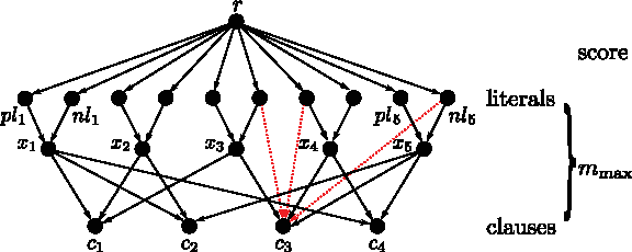For all \documentclass{aastex} \usepackage{amsbsy} \usepackage{amsfonts} \usepackage{amssymb} \usepackage{bm} \usepackage{mathrsfs} \usepackage{pifont} \usepackage{stmaryrd} \usepackage{textcomp} \usepackage{portland, xspace} \usepackage{amsmath, amsxtra} \pagestyle{empty} \DeclareMathSizes {10} {9} {7} {6} \begin{document} $$i = 1 \cdots n$$\end{document} both literal vertices corresponding to variable i are connected to variable vertex x_i. If variable x_i occurs in clause c_j, vertex x_i is connected to clause vertex c_j. The score of the transitive closure w⁺ is set to zero, except between vertex pl_i and vertex c_j if and only if literal pl_i occurs in clause c_j and between vertex nl_i and vertex c_j if and only if literal nl_i occurs in clause c_j (Fig. 7). Then w⁺ ≡ 1.

OPEN IN VIEWER

FIG. 7.

Proof of Theorem 3. Example for the construction of G for \documentclass{aastex} \usepackage{amsbsy} \usepackage{amsfonts} \usepackage{amssymb} \usepackage{bm} \usepackage{mathrsfs} \usepackage{pifont} \usepackage{stmaryrd} \usepackage{textcomp} \usepackage{portland, xspace} \usepackage{amsmath, amsxtra} \pagestyle{empty} \DeclareMathSizes {10} {9} {7} {6} \begin{document} $$\Phi = ( x_1 \vee \overline{x_2} \vee x_3 ) \land (\overline{x_1} \vee x_2 \vee x_5 )\land ( \overline{x_3} \vee x_4 \vee \overline{x_5} ) \land ( \overline{x_4} \vee x_5 \vee x_1 )$$\end{document} . Transitive edges (dotted) of weight 1 are shown exemplary for clause c₃ only.

The resulting tree has 3n + m + 1 vertices, hence the construction is polynomial. From a solution of the Max-3Sat* instance that satisfies m_max clauses we can construct a solution of the Colorful Subtree Closure instance with score m_max. To prove the forward direction, assume a truth assignment Φ satisfying m_max clauses from Φ and no truth assignment that satisfies more clauses exists. Let E′ ⊆ E(G) be the subset of edges corresponding to a subtree of G. For each satisfied clause c_j choose one arbitrary variable x_i whose literal satisfies the clause. Add edge (x_i, c_j) to E′. If the positive literal satisfies the clause add edges (pl_i, x_i) and (r, pl_i) to E′ and if the negative literal satisfies the clause add edges (nl_i, x_i) and (r, nl_i) to E′. These edges E′ compose a subtree of G with transitive closure score m_max. No subtree with higher score of the transitive closure can exist, as this would mean that a truth assignment composed of the literals used in this subtree would satisfy more than m_max clauses of the formula (variables that are not in the tree are arbitrarily chosen).

To prove the backward direction assume there is a colorful subtree T of G with maximum transitive closure m_max. T has at least m_max paths from literal vertices to clause vertices that have transitive score w⁺ ≡ 1. The truth assignment corresponding to the literal vertices of T satisfies m_max clauses of Φ. No truth assignment that satisfies more than m_max clauses is possible, as this would mean that a subtree T of G (construction see above) with higher transitive closure score exists.

Now we show that our reduction is a L-reduction. Let OPT(CSC) denote the score of the optimal solution of the Colorful Subtree Closure instance, and OPT(M3S) denote the number of satisfied clauses in the optimal solution of the Max-3Sat* instance. Since the maximum score of the Colorful Subtree Closure instance is at most m, we get OPT(CSC) ≤ m. Since at least half of the clauses of the Max-3Sat* instance can be satisfied, we have OPT(M3S) ≥ m/2. Thus, OPT(CSC) ≤ α · OPT(M3S) holds for α : = 2.

Since |c − OPT(X)| = OPT(X) − c for a maximization problem X, we have to show that OPT(M3S) − c ≤ β · (OPT(CSC) − c′). We set β : = 1, then from c′ = c and OPT(CSC) = OPT(M3S) we infer \documentclass{aastex} \usepackage{amsbsy} \usepackage{amsfonts} \usepackage{amssymb} \usepackage{bm} \usepackage{mathrsfs} \usepackage{pifont} \usepackage{stmaryrd} \usepackage{textcomp} \usepackage{portland, xspace} \usepackage{amsmath, amsxtra} \pagestyle{empty} \DeclareMathSizes {10} {9} {7} {6} \begin{document} \begin{align*}\beta \cdot ( OPT ( CSC ) - c^\prime ) = OPT ( CSC ) - c^\prime = OPT ( M3S ) - c.\end{align*}\end{document}

So, the Colorful Subtree Closure problem is MAX SNP-hard, even for colorful DAGs with binary weights.   ▪