IsoLasso: A LASSO Regression Approach to RNA-Seq Based Transcriptome Assembly

Abstract

The new second generation sequencing technology revolutionizes many biology-related research fields and poses various computational biology challenges. One of them is transcriptome assembly based on RNA-Seq data, which aims at reconstructing all full-length mRNA transcripts simultaneously from millions of short reads. In this article, we consider three objectives in transcriptome assembly: the maximization of prediction accuracy, minimization of interpretation, and maximization of completeness. The first objective, the maximization of prediction accuracy, requires that the estimated expression levels based on assembled transcripts should be as close as possible to the observed ones for every expressed region of the genome. The minimization of interpretation follows the parsimony principle to seek as few transcripts in the prediction as possible. The third objective, the maximization of completeness, requires that the maximum number of mapped reads (or “expressed segments” in gene models) be explained by (i.e., contained in) the predicted transcripts in the solution. Based on the above three objectives, we present IsoLasso, a new RNA-Seq based transcriptome assembly tool. IsoLasso is based on the well-known LASSO algorithm, a multivariate regression method designated to seek a balance between the maximization of prediction accuracy and the minimization of interpretation. By including some additional constraints in the quadratic program involved in LASSO, IsoLasso is able to make the set of assembled transcripts as complete as possible. Experiments on simulated and real RNA-Seq datasets show that IsoLasso achieves, simultaneously, higher sensitivity and precision than the state-of-art transcript assembly tools.

1. Introduction

The second generation sequencing technology has become an increasingly important tool in biological and biomedical research areas, such as individual genome sequencing (Wheeler et al., 2008), gene expression level estimation (Mortazavi et al., 2008), and comparative genomics (Holt et al., 2008). RNA-Seq, a technology to study the transcriptome via second generation sequencing, was first introduced in a series of studies in 2008 (Mortazavi et al., 2008; Wilhelm et al., 2008; Lister et al., 2008; Morin et al., 2008; Marioni et al., 2008; Cloonan et al., 2008; Nagalakshmi et al., 2008) and has quickly become widely accepted as a fundamental tool for transcriptome research (Haas and Zody, 2010; Morozova et al., 2009; Wall et al., 2009; Wang et al., 2009). The revolutionary new sequencing technology allows RNA-Seq to lower sequencing cost and increase data throughput substantially, but it also poses many challenging computational biology problems, one of which is transcriptome assembly and abundance estimation from RNA-Seq reads. A variety of new algorithms and tools have been developed for this problem (Birol et al., 2009; Yassour et al., 2009; Trapnell et al., 2010; Guttman et al., 2010; Feng et al., 2010; Trapnell et al., 2009). Some splicing site discovery tools, for example, TopHat (Trapnell et al., 2009) and SpliceMap (Au et al., 2010), identify new alternative splicing events by exploring RNA-Seq reads that span different parts of the reference genome under study. Some de novo assembly tools, such as AbySS (Birol et al., 2009), try to assemble new transcripts solely from RNA-Seq reads. Other assembly tools—including Cufflinks (Trapnell et al., 2010), Scripture (Guttman et al., 2010), and IsoInfer (Feng et al., 2010)—map reads to the reference genome and build transcript models (or isoforms) from these mapped reads.

Among these tools, IsoInfer (Feng et al., 2010) enumerates all possible “valid” isoforms and uses a quadratic program (QP) to estimate the expression levels of a given set of isoforms. IsoInfer then chooses the best subset of valid isoforms such that the estimated abundance of every “expressed segment” of the reference genome (e.g., an exon) is proportional to the observed reads falling into the segment. On the other hand, Cufflinks (Trapnell et al., 2010) assembles isoforms using a parsimony strategy (i.e., it attempts to identify the minimum number of isoforms to cover all the reads). To do this, Cufflinks decomposes the “overlap graph” of compatible reads into a smallest path cover, and then calculates the expression levels of the isoforms (i.e., paths in the cover) using the probabilistic model proposed in Jiang and Wong (2009).

The strategies that IsoInfer and Cufflinks adopted correspond to two different model selection principles: prediction accuracy and interpretation (Hastie et al., 2009). IsoInfer selects isoforms to maximize the prediction accuracy (i.e., to minimize the error or discrepancy between the predicted and observed expression levels in all expressed segments). IsoInfer employs a search algorithm similar to the “best subset variable selection” algorithm (Hocking and Leslie, 1967) to find the best subset of isoforms. However, the huge search space prevents the algorithm from doing a thorough search, and many heuristic restrictions must be applied to make the search tractable. On the other hand, Cufflinks minimizes interpretation,—(in other words, the number of variables (or isoforms) that are required to explain all the mapped reads. Here, the prediction accuracy is not considered explicitly during the transcriptome assembly process. By defining a “partial order” between reads, Cufflinks filters out “uncertain” paired-end reads which may result in a sub-optimal path cover in the solution, or miss some alternative splicing events. Finally, Scripture (Guttman et al., 2010) reconstructs all possible isoforms by enumerating all possible paths in the “connectivity graph.” This approach may lead to many incorrect isoforms for complex genes with a large number of exons, since the number of paths may be huge for such gene models.

Another important objective in transcriptome assembly is completeness, which requires that all exons (and exon junctions) appear in at least one isoform in the solution (as done in IsoInfer [Feng et al., 2010]), or all mapped reads be contained in at least one isoform (as done in Cufflinks [Trapnell et al., 2010]). In IsoInfer, the completeness is achieved by solving a set cover instance that covers all expressed segments and exon junctions. Since all the reads represented in the overlap graph are partitioned into disjoint paths in Cufflinks, they are guaranteed to be supported by at least one isoform (i.e., path). However, some “uncertain” paired-end reads (i.e., reads that cannot be included in partial order and thus absent in the overlap graph) may not be covered by the solution. Scripture adopts a conservative approach to enumerate all possible paths in its connectivity graph, which is guaranteed to cover all expressed segments and exon junctions. Like Cufflinks, the prediction accuracy is not considered explicitly during the transcript assembly process of Scripture. Moreover, retaining all possible isoforms clearly leads to a bad interpretation. Table 1 lists all the principles (or objectives) that IsoInfer, Cufflinks and Scripture abide by in the transcript assembly process.

Table 1.

Transcriptome Assembly Objectives of Each Algorithm

Algorithm	Prediction accuracy	Interpretation	Completeness
IsoInfer	Yes	Partially	Yes
Cufflinks	No	Yes	Partially
Scripture	No	No	Yes
IsoLasso	Yes	Yes	Partially

Although Cufflinks has a transcript abundance estimation step, the prediction accuracy is not considered explicitly during the assembly process. Also, theoretically both Cufflinks and IsoLasso take completeness into consideration, but in practice they may not fully guarantee it and thus are marked “partially” in the table.

In this article, we present a new isoform assembly algorithm, IsoLasso, which balances prediction accuracy, interpretation and completeness. IsoLasso uses the Least Absolute Shrinkage and Selection Operator (LASSO) algorithm (Tibshirani, 1996), which is a shrinkage least squares method in statistical machine learning. By adding an L1 norm penalty term to the least squares objective function, LASSO achieves sparsity by setting the expression levels of unrelated isoforms to zero, thus balancing both prediction accuracy and interpretation. The LASSO algorithm is widely applied in many computational biology areas, such as genome-wide association analysis (Wu et al., 2009; Kim et al., 2009), gene regulatory network (Gustafsson et al., 2005), and microarray data analysis (Ma et al., 2007). In IsoLasso, we expand the quadratic programming problem in LASSO to take completeness into consideration. Our experiments demonstrate that IsoLasso runs efficiently and achieves overall higher sensitivity and precision than IsoInfer, Cufflinks and Scripture.

The rest of this article is organized as follows. Sections 2.1 and 2.2 present our algorithm for generating (or enumerating) candidate isoforms and its relationship to minimum path covers used in Cufflinks (Trapnell et al., 2010). These candidate isoforms will be fed to our LASSO algorithm described in Section 2.3 for estimating isoform expression levels (or, equivalently, for inferring expressed isoforms). Section 2.4 expands the basic LASSO approach to take completeness into consideration. Experimental results are presented in Section 3, which include comparisons between IsoLasso, IsoInfer, Cufflinks, and Scripture on simulated and real datasets. Section 4 concludes the article.

2. Methods

2.1. Enumerating candidate isoforms

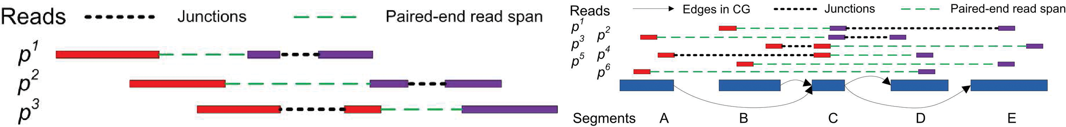
IsoInfer (Feng et al., 2010), Scripture (Guttman et al., 2010), and Cufflinks (Trapnell et al., 2010) enumerate candidate isoforms in different ways. IsoInfer, assuming that expressed segment (or exon) boundaries in a gene are given, enumerates all possible combinations of segments. Note that it is possible that some lowly expressed segment are not hit by short reads and thus many of the isoforms enumerated by IsoInfer might have very low expression levels. Scripture enumerates all possible maximal paths in a connectivity graph; but some of these isoforms may be “infeasible” because they cannot be assembled from the mapped reads (Fig. 1, right). Cufflinks tries to build an overlap graph from partially ordered reads and assembles putative transcripts by decomposing the overlap graph into a parsimonious path cover. However, a strict partial order between reads is required here. Since the actual sequence between the ends of each paired-end read is unknown, Cufflinks has to exclude some paired-end reads (called uncertain reads) to maintain the partial order. Removing uncertain reads may lead to two potential problems: (1) the path cover solution is actually sub-optimal and (2) some alternative splicing events are missed, if the reads including these events are removed. For instance, Figure 1 (left) provides an example that removing such “uncertain” reads leaves some splicing junctions undetected. Note that uncertain reads should be treated separately from repeat sequences or incorrectly mapped reads.

FIG. 1.

(Left) Removal of “uncertain” reads may cause splicing junctions undetected in Cufflinks. Three paired-end reads, p¹, p², and p³, concern different splicing junctions. Both pairs (p¹, p²) and (p², p³) are compatible, but the pair (p¹, p³) is not. Removing any of these reads will cause one or more junctions undetected. (Right) “Infeasible” paths in the connectivity graph. In the example above, there are four possible combinations of segments: ACD, ACE, BCD, and BCE. However, ACE and BCD are infeasible since they cannot be assembled from the mapped paired-end reads.

Here, we describe our method of enumerating isoforms based on the connectivity graph (Guttman et al., 2010) in Algorithm 1, from which the enumerated isoforms will be the set of candidate isoforms to be considered in the LASSO algorithm. The algorithm first enumerates isoforms from the connectivity graph as in Guttman et al. (2010) and then uses two additional steps to remove isoforms that are impossible to assemble. We will prove some important properties of Algorithm 1: if there are no “uncertain” reads, then every isoform output by Algorithm 1 can be assembled from a maximal path in the overlap graph given in (Trapnell et al. (2010). Moreover, the isoforms enumerated by Algorithm 1 form a superset of all possible maximal paths in the overlap graph. In other words, our LASSO algorithm in general considers more isoforms than Cufflinks in the transcript assembly process. Before giving a detailed description of this algorithm and proofs of these properties, we first briefly review some necessary notations first introduced in Trapnell et al. (2010) and Guttman et al. (2010).

A gene sequence S of length n is an ordered character sequence \documentclass{aastex}\usepackage{amsbsy}\usepackage{amsfonts}\usepackage{amssymb}\usepackage{bm}\usepackage{mathrsfs}\usepackage{pifont}\usepackage{stmaryrd}\usepackage{textcomp}\usepackage{portland, xspace}\usepackage{amsmath, amsxtra}\pagestyle{empty}\DeclareMathSizes{10}{9}{7}{6}\begin{document}$$S = S_1S_2 \cdots S_n , S_i \in \{ A , T , G , C \} $$\end{document} . Define B(n) as the set of binary vectors of length n. For a vector \documentclass{aastex}\usepackage{amsbsy}\usepackage{amsfonts}\usepackage{amssymb}\usepackage{bm}\usepackage{mathrsfs}\usepackage{pifont}\usepackage{stmaryrd}\usepackage{textcomp}\usepackage{portland, xspace}\usepackage{amsmath, amsxtra}\pagestyle{empty}\DeclareMathSizes{10}{9}{7}{6}\begin{document}$$b \in B ( n )$$\end{document} , b_i indicates the ith element of vector b. For a subset U ⊂ B(n), define \documentclass{aastex}\usepackage{amsbsy}\usepackage{amsfonts}\usepackage{amssymb}\usepackage{bm}\usepackage{mathrsfs}\usepackage{pifont}\usepackage{stmaryrd}\usepackage{textcomp}\usepackage{portland, xspace}\usepackage{amsmath, amsxtra}\pagestyle{empty}\DeclareMathSizes{10}{9}{7}{6}\begin{document}$$OR ( U ) = b \in B ( n )$$\end{document} with b_i = 1 iff there is an element \documentclass{aastex}\usepackage{amsbsy}\usepackage{amsfonts}\usepackage{amssymb}\usepackage{bm}\usepackage{mathrsfs}\usepackage{pifont}\usepackage{stmaryrd}\usepackage{textcomp}\usepackage{portland, xspace}\usepackage{amsmath, amsxtra}\pagestyle{empty}\DeclareMathSizes{10}{9}{7}{6}\begin{document}$$c \in U$$\end{document} such that c_i = 1. For a binary vector \documentclass{aastex}\usepackage{amsbsy}\usepackage{amsfonts}\usepackage{amssymb}\usepackage{bm}\usepackage{mathrsfs}\usepackage{pifont}\usepackage{stmaryrd}\usepackage{textcomp}\usepackage{portland, xspace}\usepackage{amsmath, amsxtra}\pagestyle{empty}\DeclareMathSizes{10}{9}{7}{6}\begin{document}$$b \in B ( n )$$\end{document} , define the start (or end) of b as the first (or last) non-zero index of b, and is denoted as l(b) (or u(b)). Hence, each isoform on gene S could be represented as a binary vector \documentclass{aastex}\usepackage{amsbsy}\usepackage{amsfonts}\usepackage{amssymb}\usepackage{bm}\usepackage{mathrsfs}\usepackage{pifont}\usepackage{stmaryrd}\usepackage{textcomp}\usepackage{portland, xspace}\usepackage{amsmath, amsxtra}\pagestyle{empty}\DeclareMathSizes{10}{9}{7}{6}\begin{document}$$b \in B ( n )$$\end{document} with b_i = 1 iff the nucleotide S_i is included in this isoform. A single-end or paired-end read mapped to S could also be represented as an element \documentclass{aastex}\usepackage{amsbsy}\usepackage{amsfonts}\usepackage{amssymb}\usepackage{bm}\usepackage{mathrsfs}\usepackage{pifont}\usepackage{stmaryrd}\usepackage{textcomp}\usepackage{portland, xspace}\usepackage{amsmath, amsxtra}\pagestyle{empty}\DeclareMathSizes{10}{9}{7}{6}\begin{document}$$b \in B ( n )$$\end{document} with b_i = 1 iff this read contains S_i. A paired-end read is denoted as p = (b¹, b²), where b¹ and b² are the two mapped single-end reads, and l(b¹) < l(b²). Given a set of single-end or paired-end reads R, the coverage of S_i, or cvg(S_i), is the number of reads b with b_i = 1.

A single-end read b is compatible with an isoform t, denoted as b∼t, iff b_i = t_i for l(b) ≤ i ≤ u(b). Similarly, a paired-end read p = (b¹,b²) is compatible with isoform t, denoted as p ∼ t, iff b¹ ∼ t and b² ∼ t. Given a set of single-end (or paired-end) reads R mapped to gene S, the connectivity graph (CG) (Guttman et al., 2010) is a directed acyclic graph (DAG) G = (V, E), where \documentclass{aastex}\usepackage{amsbsy}\usepackage{amsfonts}\usepackage{amssymb}\usepackage{bm}\usepackage{mathrsfs}\usepackage{pifont}\usepackage{stmaryrd}\usepackage{textcomp}\usepackage{portland, xspace}\usepackage{amsmath, amsxtra}\pagestyle{empty}\DeclareMathSizes{10}{9}{7}{6}\begin{document}$$V = \{ v_1 , v_2 , \ldots , v_n \} $$\end{document} and \documentclass{aastex}\usepackage{amsbsy}\usepackage{amsfonts}\usepackage{amssymb}\usepackage{bm}\usepackage{mathrsfs}\usepackage{pifont}\usepackage{stmaryrd}\usepackage{textcomp}\usepackage{portland, xspace}\usepackage{amsmath, amsxtra}\pagestyle{empty}\DeclareMathSizes{10}{9}{7}{6}\begin{document}$$e = ( v_i , v_j ) \in E$$\end{document} iff one of the following conditions is true:

Condition 1. There exists a single-end read or an end of some paired-end read \documentclass{aastex}\usepackage{amsbsy}\usepackage{amsfonts}\usepackage{amssymb}\usepackage{bm}\usepackage{mathrsfs}\usepackage{pifont}\usepackage{stmaryrd}\usepackage{textcomp}\usepackage{portland, xspace}\usepackage{amsmath, amsxtra}\pagestyle{empty}\DeclareMathSizes{10}{9}{7}{6}\begin{document}$$b \in R$$\end{document} such that b_i = 1, b_j = 1, and b_k = 0, ∀i < k < j;

Condition 2. cvg(S_i) > 0, cvg(S_j) > 0, and cvg(S_k) = 0, ∀i < k < j.

Note that Condition 2 is designed to connect two mapped reads separated by a coverage gap. Based on the definition of CG, a path h in the CG could be readily treated as an isoform by defining the isoform t as t_i = 1 iff \documentclass{aastex}\usepackage{amsbsy}\usepackage{amsfonts}\usepackage{amssymb}\usepackage{bm}\usepackage{mathrsfs}\usepackage{pifont}\usepackage{stmaryrd}\usepackage{textcomp}\usepackage{portland, xspace}\usepackage{amsmath, amsxtra}\pagestyle{empty}\DeclareMathSizes{10}{9}{7}{6}\begin{document}$$v_i \in h$$\end{document} . Therefore, a read b is compatible with h (denoted as b ∼ h) iff b ∼ t. The isoform enumeration algorithm depicted in Algorithm 1 takes the connectivity graph as the input, and outputs a set of maximal candidate isoforms T. The algorithm consists of three phases: Enumeration, Filtration, and Condensation. In the Enumeration phase, all maximal paths in the connectivity graph are enumerated. However, some of these isoforms are “infeasible” in the sense that they cannot be assembled from the mapped reads (Fig. 1, right). In this case, the second phase (i.e., the Filtration phase) is required to remove such isoforms. For each isoform t generated in the Enumeration phase, the Filtration phase first finds all reads that are compatible with t, and then checks if t can be assembled from these compatible reads (it replaces t otherwise). Finally, the Condensation phase removes all the isoforms that are not maximal candidates.

Algorithm 1

Isoform Enumeration

input: A CG G = (V, E), and a set of mapped single-end or paired-end reads R

output: A set of isoforms T

begin

Enumeration:

T ← ∅

for

\documentclass{aastex}\usepackage{amsbsy}\usepackage{amsfonts}\usepackage{amssymb}\usepackage{bm}\usepackage{mathrsfs}\usepackage{pifont}\usepackage{stmaryrd}\usepackage{textcomp}\usepackage{portland, xspace}\usepackage{amsmath, amsxtra}\pagestyle{empty}\DeclareMathSizes{10}{9}{7}{6}\begin{document}$$v_j \in V$$\end{document}

with indeg(v_j) = 0 do

Enumerate all possible maximal paths P that begin at v_j and end at some v_k with outdeg(v_k) = 0

T ← T ∪ P

Filtration:

for

Let

T ← (T\{t}) ∪ {t′}

Condensation:

for

Let

for

Let

then

T ← (T\{t})

2.2. A connection to Cufflinks

Cufflinks assembles transcripts based on the overlap graph (OG), which is constructed from a set of mapped single-end or paired-end reads after removing uncertain reads and extending reads to include their nested reads (Trapnell et al., 2010). It generates transcripts by partitioning the overlap graph into a minimum path cover, where a path cover is a set of disjoint paths in the overlap graph such that every read appears in one and only one path. A minimum path cover is a path cover with the minimum number of paths. We will prove some theorems to establish the relationship between the set of isoforms generated by Algorithm 1 and the set of transcripts that could be constructed from the overlap graph.

The formal definitions of uncertain reads, nested reads, and the overlap graph are given in Trapnell et al. (2010) and are reviewed below for the reader's convenience.

A single-end read b is nested in another single-end read b′ iff \documentclass{aastex}\usepackage{amsbsy}\usepackage{amsfonts}\usepackage{amssymb}\usepackage{bm}\usepackage{mathrsfs}\usepackage{pifont}\usepackage{stmaryrd}\usepackage{textcomp}\usepackage{portland, xspace}\usepackage{amsmath, amsxtra}\pagestyle{empty}\DeclareMathSizes{10}{9}{7}{6}\begin{document}$$b_i = b^{ \prime}_i , l ( b ) \leq i \leq u ( b )$$\end{document} , and at least one of the following two conditions is true: (1) l(b) ≠ l(b′) and (2) u(b) ≠ u(b′). A paired-end read p is nested in another paired-end read p′ iff l(p) ≥ l(p′), u(p) ≤ u(p′) and at least one of the following conditions is true: (1) l(p) ≠ l(p′) and (2) u(p) ≠ u(p′). If a single-end read b is nested in b′, b can always be removed safely without losing any information.

Two single-end reads b and b′ are compatible, denoted as b ∼ b′, iff there exists one isoform t such that b ∼ t, b′ ∼ t, and b and b′ are not nested to each other. If b and b′ are not compatible, we denote b ≁ b′. Two paired-end reads p and p′ are compatible, denoted as p ∼ p′, iff there exists an isoform t such that p ∼ t, p′ ∼ t and p is not nested in p′ or vice versa. If p and p′ are not compatible, we denote p ≁ p′.

Define a partial order ≤ between two single-end reads b and b′: b ≤ b′ iff b ∼ b′ and l(b) ≤ l(b′). It is impossible to extend the partial order to paired-end reads, since the sequence within a paired-end read is not completely known. Alternatively, for two paired-end reads p and p′, define p ≤ p′ with respect to a given read set R iff the following conditions are true: (1) p ∼ p′, (2) l(p) ≤ l(p′), u(p) ≤ u(p′), and (3) there is no paired-end read \documentclass{aastex}\usepackage{amsbsy}\usepackage{amsfonts}\usepackage{amssymb}\usepackage{bm}\usepackage{mathrsfs}\usepackage{pifont}\usepackage{stmaryrd}\usepackage{textcomp}\usepackage{portland, xspace}\usepackage{amsmath, amsxtra}\pagestyle{empty}\DeclareMathSizes{10}{9}{7}{6}\begin{document}$$p^{ \prime \prime} \in R$$\end{document} such that p ∼ p′, p ∼ p″ but p ≁ p″. Write p ≤ p″|R if p ≤ p′ with respect to a given read set R, or write simply p ≤ p′ if there is no ambiguity. If reads p, p′ and p″ exist such that p ∼ p′, p′ ∼ p″ and p ≁ p″, then p, p′ and p″ are said to be uncertain since no partial order can be given to these reads.

Given a set of mapped single-end or paired-end reads \documentclass{aastex}\usepackage{amsbsy}\usepackage{amsfonts}\usepackage{amssymb}\usepackage{bm}\usepackage{mathrsfs}\usepackage{pifont}\usepackage{stmaryrd}\usepackage{textcomp}\usepackage{portland, xspace}\usepackage{amsmath, amsxtra}\pagestyle{empty}\DeclareMathSizes{10}{9}{7}{6}\begin{document}$$R = \{ b^1 , b^2 , \ldots \} $$\end{document} , the overlap graph (OG) (Trapnell et al., 2010) is a DAG G = (V, E), where \documentclass{aastex}\usepackage{amsbsy}\usepackage{amsfonts}\usepackage{amssymb}\usepackage{bm}\usepackage{mathrsfs}\usepackage{pifont}\usepackage{stmaryrd}\usepackage{textcomp}\usepackage{portland, xspace}\usepackage{amsmath, amsxtra}\pagestyle{empty}\DeclareMathSizes{10}{9}{7}{6}\begin{document}$$V = \{ v_1 , v_2 , \ldots , v_{ \mid R \mid } \} $$\end{document} and \documentclass{aastex}\usepackage{amsbsy}\usepackage{amsfonts}\usepackage{amssymb}\usepackage{bm}\usepackage{mathrsfs}\usepackage{pifont}\usepackage{stmaryrd}\usepackage{textcomp}\usepackage{portland, xspace}\usepackage{amsmath, amsxtra}\pagestyle{empty}\DeclareMathSizes{10}{9}{7}{6}\begin{document}$$e = ( v_i , v_j ) \in E$$\end{document} iff bⁱ ≤ b^j. A maximal path of length k on the OG is a path \documentclass{aastex}\usepackage{amsbsy}\usepackage{amsfonts}\usepackage{amssymb}\usepackage{bm}\usepackage{mathrsfs}\usepackage{pifont}\usepackage{stmaryrd}\usepackage{textcomp}\usepackage{portland, xspace}\usepackage{amsmath, amsxtra}\pagestyle{empty}\DeclareMathSizes{10}{9}{7}{6}\begin{document}$$h = \{ v_{i_1} \le v_{i_2} \le \cdots \le v_{i_k} \} $$\end{document} on the OG, such that there exists no path \documentclass{aastex}\usepackage{amsbsy}\usepackage{amsfonts}\usepackage{amssymb}\usepackage{bm}\usepackage{mathrsfs}\usepackage{pifont}\usepackage{stmaryrd}\usepackage{textcomp}\usepackage{portland, xspace}\usepackage{amsmath, amsxtra}\pagestyle{empty}\DeclareMathSizes{10}{9}{7}{6}\begin{document}$$h^{ \prime} = \left\{ v_{j_1} \le v_{j_2} \le \cdots \le v_{j_{k^{ \prime}}} \right\} $$\end{document} with h ⊂ h′. Because the vertices in the OG have a one-to-one relationship with the mapped reads, we also treat vertices in the OG as binary vectors to simplify notations below. For example, if a path \documentclass{aastex}\usepackage{amsbsy}\usepackage{amsfonts}\usepackage{amssymb}\usepackage{bm}\usepackage{mathrsfs}\usepackage{pifont}\usepackage{stmaryrd}\usepackage{textcomp}\usepackage{portland, xspace}\usepackage{amsmath, amsxtra}\pagestyle{empty}\DeclareMathSizes{10}{9}{7}{6}\begin{document}$$h = \left\{ v_{i_1} \le v_{i_2} \le \cdots \le v_{i_k} \right\} $$\end{document} , we will use OR(h) to denote \documentclass{aastex}\usepackage{amsbsy}\usepackage{amsfonts}\usepackage{amssymb}\usepackage{bm}\usepackage{mathrsfs}\usepackage{pifont}\usepackage{stmaryrd}\usepackage{textcomp}\usepackage{portland, xspace}\usepackage{amsmath, amsxtra}\pagestyle{empty}\DeclareMathSizes{10}{9}{7}{6}\begin{document}$$OR ( \{ b^{i_1} \le b^{i_2} \le \cdots \le b^{i_k} \} )$$\end{document} .

Let us consider a fixed gene S. Suppose that R is the set of reads mapped to gene S. The following lemmas will be useful.

Lemma 1

Denote the vertex set of the CG as \documentclass{aastex}\usepackage{amsbsy}\usepackage{amsfonts}\usepackage{amssymb}\usepackage{bm}\usepackage{mathrsfs}\usepackage{pifont}\usepackage{stmaryrd}\usepackage{textcomp}\usepackage{portland, xspace}\usepackage{amsmath, amsxtra}\pagestyle{empty}\DeclareMathSizes{10}{9}{7}{6}\begin{document}$$V = \{ v_1 , v_2 , \ldots , v_n \} $$\end{document} . For 1 ≤ i < j ≤ n, there is a path from v_i to v_j if cvg(S_i) > 0 and cvg(S_j) > 0.

Proof

We use an induction on n = j − i to prove this lemma. If j − i = 1, then there is an edge between v_i and v_j by Condition 2 of the CG's edge construction. Assume that ∀k < n, there is a path from v_i to v_j if cvg(S_i) > 0 and cvg(S_j) > 0, j − i = k. For k = n, if cvg(S_l) = 0 for every i < l < j, then there is an edge between v_i and v_j by Condition 2 of the CG's edge construction. Otherwise, if there exists i < l′ < j such that \documentclass{aastex}\usepackage{amsbsy}\usepackage{amsfonts}\usepackage{amssymb}\usepackage{bm}\usepackage{mathrsfs}\usepackage{pifont}\usepackage{stmaryrd}\usepackage{textcomp}\usepackage{portland, xspace}\usepackage{amsmath, amsxtra}\pagestyle{empty}\DeclareMathSizes{10}{9}{7}{6}\begin{document}$$cvg ( S_{l^{ \prime}} ) > 0$$\end{document} , then l′ − i < n and j − l′ < n. Using the assumption above, there is a path from v_i to \documentclass{aastex}\usepackage{amsbsy}\usepackage{amsfonts}\usepackage{amssymb}\usepackage{bm}\usepackage{mathrsfs}\usepackage{pifont}\usepackage{stmaryrd}\usepackage{textcomp}\usepackage{portland, xspace}\usepackage{amsmath, amsxtra}\pagestyle{empty}\DeclareMathSizes{10}{9}{7}{6}\begin{document}$$v_{l^{ \prime}}$$\end{document} and a path from \documentclass{aastex}\usepackage{amsbsy}\usepackage{amsfonts}\usepackage{amssymb}\usepackage{bm}\usepackage{mathrsfs}\usepackage{pifont}\usepackage{stmaryrd}\usepackage{textcomp}\usepackage{portland, xspace}\usepackage{amsmath, amsxtra}\pagestyle{empty}\DeclareMathSizes{10}{9}{7}{6}\begin{document}$$v_{l^{ \prime}}$$\end{document} to v_j. Therefore, there is a path from v_i to v_j. ▪

Lemma 2

For any read set Q ⊆ R, if every two reads in Q are compatible, then there is a maximal path h in the CG such that \documentclass{aastex}\usepackage{amsbsy}\usepackage{amsfonts}\usepackage{amssymb}\usepackage{bm}\usepackage{mathrsfs}\usepackage{pifont}\usepackage{stmaryrd}\usepackage{textcomp}\usepackage{portland, xspace}\usepackage{amsmath, amsxtra}\pagestyle{empty}\DeclareMathSizes{10}{9}{7}{6}\begin{document}$$\forall b \in Q , b \sim h$$\end{document} .

Proof

Let t = OR(Q). We construct h by defining its vertex set V (h) and edge set E(h) separately. For every 1 ≤ i < m,t_i = 1, if the set {k > i|t_k = 1} is not empty, denote j = min_k{k > i,t_k = 1}. If there is a read \documentclass{aastex}\usepackage{amsbsy}\usepackage{amsfonts}\usepackage{amssymb}\usepackage{bm}\usepackage{mathrsfs}\usepackage{pifont}\usepackage{stmaryrd}\usepackage{textcomp}\usepackage{portland, xspace}\usepackage{amsmath, amsxtra}\pagestyle{empty}\DeclareMathSizes{10}{9}{7}{6}\begin{document}$$b \in Q$$\end{document} such that b_i = b_j = 1 and b_k = 0, i < k < j, then there must be an edge e in CG from v_i to v_j by Condition 2 of CG's edge construction, and we put e in E(h). Otherwise, there must be a path h′ from v_i to v_j by Lemma 1, because cvg(S_i) > 0 and cvg(S_j) > 0. We put edges in h′ in E(h). Define V (h) as the set of vertices induced by E(h). A trivial case is that |{1 ≤ i < m,t_i = 1}| = 1. In this case, let V (h) = v_i,t_i = 1 for completeness.

We claim that all reads in Q are compatible with h. This is because for a single-end read (or an end of some paired-end read) b in Q, if b_i = 1 then \documentclass{aastex}\usepackage{amsbsy}\usepackage{amsfonts}\usepackage{amssymb}\usepackage{bm}\usepackage{mathrsfs}\usepackage{pifont}\usepackage{stmaryrd}\usepackage{textcomp}\usepackage{portland, xspace}\usepackage{amsmath, amsxtra}\pagestyle{empty}\DeclareMathSizes{10}{9}{7}{6}\begin{document}$$v_i \in V ( h )$$\end{document} . If b_i = b_j = 1 and b_k = 0,i < k < j, v_i and v_j are directly connected by edge (v_i, v_j) in h, which means that {v_k|i < k < j} ∩ V (h) = ∅. Therefore, b ∼ h.

Once h is obtained, it is easily extended to a maximal path without violating its compatibility with every read in Q. ▪

Lemma 3

Suppose that R has no uncertain or nested reads. For every maximal path h on the OG constructed based on R, \documentclass{aastex}\usepackage{amsbsy}\usepackage{amsfonts}\usepackage{amssymb}\usepackage{bm}\usepackage{mathrsfs}\usepackage{pifont}\usepackage{stmaryrd}\usepackage{textcomp}\usepackage{portland, xspace}\usepackage{amsmath, amsxtra}\pagestyle{empty}\DeclareMathSizes{10}{9}{7}{6}\begin{document}$$OR ( h ) \in T$$\end{document} .

Proof

Let t = OR(h) and R_t be the set of reads corresponding to path h. By Lemma 2, there is a maximal path h′ on the CG such that every read \documentclass{aastex}\usepackage{amsbsy}\usepackage{amsfonts}\usepackage{amssymb}\usepackage{bm}\usepackage{mathrsfs}\usepackage{pifont}\usepackage{stmaryrd}\usepackage{textcomp}\usepackage{portland, xspace}\usepackage{amsmath, amsxtra}\pagestyle{empty}\DeclareMathSizes{10}{9}{7}{6}\begin{document}$$b \in R_t$$\end{document} is compatible with h′. Denote the isoform corresponding to h′ as t′. Then, \documentclass{aastex}\usepackage{amsbsy}\usepackage{amsfonts}\usepackage{amssymb}\usepackage{bm}\usepackage{mathrsfs}\usepackage{pifont}\usepackage{stmaryrd}\usepackage{textcomp}\usepackage{portland, xspace}\usepackage{amsmath, amsxtra}\pagestyle{empty}\DeclareMathSizes{10}{9}{7}{6}\begin{document}$$t^{ \prime} \in T$$\end{document} after the Enumeration phase of Algorithm 1 and b ∼ t′.

Let \documentclass{aastex}\usepackage{amsbsy}\usepackage{amsfonts}\usepackage{amssymb}\usepackage{bm}\usepackage{mathrsfs}\usepackage{pifont}\usepackage{stmaryrd}\usepackage{textcomp}\usepackage{portland, xspace}\usepackage{amsmath, amsxtra}\pagestyle{empty}\DeclareMathSizes{10}{9}{7}{6}\begin{document}$$R_{t^{ \prime}} = \{ b \in R \mid b \sim t^{ \prime} \} $$\end{document} . For any \documentclass{aastex}\usepackage{amsbsy}\usepackage{amsfonts}\usepackage{amssymb}\usepackage{bm}\usepackage{mathrsfs}\usepackage{pifont}\usepackage{stmaryrd}\usepackage{textcomp}\usepackage{portland, xspace}\usepackage{amsmath, amsxtra}\pagestyle{empty}\DeclareMathSizes{10}{9}{7}{6}\begin{document}$$b \in R_t , b \sim t^{ \prime}$$\end{document} so \documentclass{aastex}\usepackage{amsbsy}\usepackage{amsfonts}\usepackage{amssymb}\usepackage{bm}\usepackage{mathrsfs}\usepackage{pifont}\usepackage{stmaryrd}\usepackage{textcomp}\usepackage{portland, xspace}\usepackage{amsmath, amsxtra}\pagestyle{empty}\DeclareMathSizes{10}{9}{7}{6}\begin{document}$$b \in R_{t^{ \prime}}$$\end{document} , then we have \documentclass{aastex}\usepackage{amsbsy}\usepackage{amsfonts}\usepackage{amssymb}\usepackage{bm}\usepackage{mathrsfs}\usepackage{pifont}\usepackage{stmaryrd}\usepackage{textcomp}\usepackage{portland, xspace}\usepackage{amsmath, amsxtra}\pagestyle{empty}\DeclareMathSizes{10}{9}{7}{6}\begin{document}$$R_t \subseteq R_{t^{ \prime}}$$\end{document} . Furthermore, for any \documentclass{aastex}\usepackage{amsbsy}\usepackage{amsfonts}\usepackage{amssymb}\usepackage{bm}\usepackage{mathrsfs}\usepackage{pifont}\usepackage{stmaryrd}\usepackage{textcomp}\usepackage{portland, xspace}\usepackage{amsmath, amsxtra}\pagestyle{empty}\DeclareMathSizes{10}{9}{7}{6}\begin{document}$$b^{ \prime} \in R_{t^{ \prime}} , b^{ \prime} \sim t^{ \prime}$$\end{document} , and thus we have \documentclass{aastex}\usepackage{amsbsy}\usepackage{amsfonts}\usepackage{amssymb}\usepackage{bm}\usepackage{mathrsfs}\usepackage{pifont}\usepackage{stmaryrd}\usepackage{textcomp}\usepackage{portland, xspace}\usepackage{amsmath, amsxtra}\pagestyle{empty}\DeclareMathSizes{10}{9}{7}{6}\begin{document}$$b \sim b^{ \prime} , \forall b \in R_t , \forall b^{ \prime} \in R_{t^{ \prime}}$$\end{document} . If there is a read \documentclass{aastex}\usepackage{amsbsy}\usepackage{amsfonts}\usepackage{amssymb}\usepackage{bm}\usepackage{mathrsfs}\usepackage{pifont}\usepackage{stmaryrd}\usepackage{textcomp}\usepackage{portland, xspace}\usepackage{amsmath, amsxtra}\pagestyle{empty}\DeclareMathSizes{10}{9}{7}{6}\begin{document}$$b \in R_{t^{ \prime}}$$\end{document} but \documentclass{aastex}\usepackage{amsbsy}\usepackage{amsfonts}\usepackage{amssymb}\usepackage{bm}\usepackage{mathrsfs}\usepackage{pifont}\usepackage{stmaryrd}\usepackage{textcomp}\usepackage{portland, xspace}\usepackage{amsmath, amsxtra}\pagestyle{empty}\DeclareMathSizes{10}{9}{7}{6}\begin{document}$$b \notin R_t$$\end{document} , the vertex corresponding to b in the OG could be added to path h, because b is compatible with all the reads in R_t and b is not a nested or uncertain read. However, this contradicts the assumption that h is maximal. Therefore, \documentclass{aastex}\usepackage{amsbsy}\usepackage{amsfonts}\usepackage{amssymb}\usepackage{bm}\usepackage{mathrsfs}\usepackage{pifont}\usepackage{stmaryrd}\usepackage{textcomp}\usepackage{portland, xspace}\usepackage{amsmath, amsxtra}\pagestyle{empty}\DeclareMathSizes{10}{9}{7}{6}\begin{document}$$R_t = R_{t^{ \prime}}$$\end{document} and \documentclass{aastex}\usepackage{amsbsy}\usepackage{amsfonts}\usepackage{amssymb}\usepackage{bm}\usepackage{mathrsfs}\usepackage{pifont}\usepackage{stmaryrd}\usepackage{textcomp}\usepackage{portland, xspace}\usepackage{amsmath, amsxtra}\pagestyle{empty}\DeclareMathSizes{10}{9}{7}{6}\begin{document}$$t \in T$$\end{document} after the Filtration phase of Algorithm 1. Note that t would not be removed in the Condensation phase Algorithm 1 because t is maximal. ▪

Lemma 4

Suppose that R has no uncertain or nested reads. For every isoform t output by Algorithm 1, there exists a maximal path h on the OG such that OR(h) = t.

Proof

Let t be an isoform enumerated by Algorithm 1 and \documentclass{aastex}\usepackage{amsbsy}\usepackage{amsfonts}\usepackage{amssymb}\usepackage{bm}\usepackage{mathrsfs}\usepackage{pifont}\usepackage{stmaryrd}\usepackage{textcomp}\usepackage{portland, xspace}\usepackage{amsmath, amsxtra}\pagestyle{empty}\DeclareMathSizes{10}{9}{7}{6}\begin{document}$$R_t = \{ b \in R \mid b \sim t \} $$\end{document} . Since R contains no uncertain or nested reads, the vertices corresponding to R_t in the OG form a path h. If h is not maximal, it can be “expanded” to a maximal path h′ by adding some vertices not in h. According to Lemma 3, there is an isoform \documentclass{aastex}\usepackage{amsbsy}\usepackage{amsfonts}\usepackage{amssymb}\usepackage{bm}\usepackage{mathrsfs}\usepackage{pifont}\usepackage{stmaryrd}\usepackage{textcomp}\usepackage{portland, xspace}\usepackage{amsmath, amsxtra}\pagestyle{empty}\DeclareMathSizes{10}{9}{7}{6}\begin{document}$$t^{ \prime} \in T$$\end{document} such that t′ = OR(h′). Denoting \documentclass{aastex}\usepackage{amsbsy}\usepackage{amsfonts}\usepackage{amssymb}\usepackage{bm}\usepackage{mathrsfs}\usepackage{pifont}\usepackage{stmaryrd}\usepackage{textcomp}\usepackage{portland, xspace}\usepackage{amsmath, amsxtra}\pagestyle{empty}\DeclareMathSizes{10}{9}{7}{6}\begin{document}$$R_{t^{ \prime}} = \{ b \in R \mid b \sim t^{ \prime} \} $$\end{document} , then we have \documentclass{aastex}\usepackage{amsbsy}\usepackage{amsfonts}\usepackage{amssymb}\usepackage{bm}\usepackage{mathrsfs}\usepackage{pifont}\usepackage{stmaryrd}\usepackage{textcomp}\usepackage{portland, xspace}\usepackage{amsmath, amsxtra}\pagestyle{empty}\DeclareMathSizes{10}{9}{7}{6}\begin{document}$$R_t \subset R_{t^{ \prime}}$$\end{document} . Therefore, t would be removed in the Condensation phase of Algorithm 1, which contradicts the fact that t is output by Algorithm 1. ▪

Lemmas 3 and 4 immediately lead to Theorem 1 and its corollary, Corollary 1, below.

Theorem 1

Suppose that R contains no uncertain or nested reads. If we denote the set of isoforms constructed by Algorithm 1 as T and the set of the isoforms formed by enumerating maximal paths on the OG (constructed from R) as T_OG, then T = T_OG.

Corollary 1

If R contains no uncertain or nested reads, then for every minimum path cover H of the OG, there exists a set of maximal isoforms \documentclass{aastex}\usepackage{amsbsy}\usepackage{amsfonts}\usepackage{amssymb}\usepackage{bm}\usepackage{mathrsfs}\usepackage{pifont}\usepackage{stmaryrd}\usepackage{textcomp}\usepackage{portland, xspace}\usepackage{amsmath, amsxtra}\pagestyle{empty}\DeclareMathSizes{10}{9}{7}{6}\begin{document}$$T^{ \prime} = \left\{ t^1 , \ldots t^m \right\} \subset T$$\end{document} such that m = |H| and for every read b on a path \documentclass{aastex}\usepackage{amsbsy}\usepackage{amsfonts}\usepackage{amssymb}\usepackage{bm}\usepackage{mathrsfs}\usepackage{pifont}\usepackage{stmaryrd}\usepackage{textcomp}\usepackage{portland, xspace}\usepackage{amsmath, amsxtra}\pagestyle{empty}\DeclareMathSizes{10}{9}{7}{6}\begin{document}$$h \in H , b \sim t^i , 1 \le i \le m$$\end{document}

Note that each nested read r in R is removed in Trapnell et al. (2010) by extending the reads that r is nested in. On the other hand, if there are uncertain reads in R, Algorithm 1 may generate some isoforms that do not correspond to any paths on the OG when these uncertain reads cover some unique splicing junctions as shown in Figure 1 (left). The following theorem states the relationship between maximal paths on the OG and the isoforms generated by Algorithm 1 when uncertain reads are present in R.

Theorem 2

Suppose that no reads in R are nested and denote the set of isoforms constructed by Algorithm 1 as T. For every maximal path h on the OG constructed by removing uncertain reads in R, T contains an isoform which is compatible with every read on the path h.

Proof

The proof is similar to the proof of Lemma 3. Let t = OR(h) and \documentclass{aastex}\usepackage{amsbsy}\usepackage{amsfonts}\usepackage{amssymb}\usepackage{bm}\usepackage{mathrsfs}\usepackage{pifont}\usepackage{stmaryrd}\usepackage{textcomp}\usepackage{portland, xspace}\usepackage{amsmath, amsxtra}\pagestyle{empty}\DeclareMathSizes{10}{9}{7}{6}\begin{document}$$1 \leq \,l_1 < l_2 < \cdots < l_m \leq \,n$$\end{document} be indices in t such that t_i = 1 iff and only if \documentclass{aastex}\usepackage{amsbsy}\usepackage{amsfonts}\usepackage{amssymb}\usepackage{bm}\usepackage{mathrsfs}\usepackage{pifont}\usepackage{stmaryrd}\usepackage{textcomp}\usepackage{portland, xspace}\usepackage{amsmath, amsxtra}\pagestyle{empty}\DeclareMathSizes{10}{9}{7}{6}\begin{document}$$i \in \{ l_1 , l_2 , \ldots , l_m \} $$\end{document} . Let R_t be the set of reads corresponding to path h. By Lemma 2, there is a maximal path h′ on the CG such that every read \documentclass{aastex}\usepackage{amsbsy}\usepackage{amsfonts}\usepackage{amssymb}\usepackage{bm}\usepackage{mathrsfs}\usepackage{pifont}\usepackage{stmaryrd}\usepackage{textcomp}\usepackage{portland, xspace}\usepackage{amsmath, amsxtra}\pagestyle{empty}\DeclareMathSizes{10}{9}{7}{6}\begin{document}$$b \in R_t$$\end{document} is compatible with h′. Denote the isoform corresponding to h′ as t′. Therefore, \documentclass{aastex}\usepackage{amsbsy}\usepackage{amsfonts}\usepackage{amssymb}\usepackage{bm}\usepackage{mathrsfs}\usepackage{pifont}\usepackage{stmaryrd}\usepackage{textcomp}\usepackage{portland, xspace}\usepackage{amsmath, amsxtra}\pagestyle{empty}\DeclareMathSizes{10}{9}{7}{6}\begin{document}$$t^{ \prime} \in T$$\end{document} after the Enumeration phase of Algorithm 1 and b ∼ t′.

During the Condensation phase of Algorithm 1, if t″ is not removed, the theorem holds. Otherwise, there must be another \documentclass{aastex}\usepackage{amsbsy}\usepackage{amsfonts}\usepackage{amssymb}\usepackage{bm}\usepackage{mathrsfs}\usepackage{pifont}\usepackage{stmaryrd}\usepackage{textcomp}\usepackage{portland, xspace}\usepackage{amsmath, amsxtra}\pagestyle{empty}\DeclareMathSizes{10}{9}{7}{6}\begin{document}$$t^{ \prime \prime \prime} \in T$$\end{document} such that all reads compatible with t″ are also compatible with t′″. In other words, all reads in R_t would be compatible with t′″. ▪

2.3. The LASSO approach of estimating isoform expression levels

2.3.1. The mathematical model of RNA-Seq

Typical alternative splicing (AS) events include alternative 5′ (or 3′) splice sites, exon skipping, intron retention, and mutually exclusive exons, but all these events can be dealt with in a unified mathematical model where a gene is partitioned into a sequence of expressed segments (or simply segments) based on exon-intron boundaries (Feng et al., 2010). More precisely, a gene is divided into a set of segments such that every segment is a continuous region in the reference genome uninterrupted by exon-intron boundaries. Then, a given set of candidate isoforms \documentclass{aastex}\usepackage{amsbsy}\usepackage{amsfonts}\usepackage{amssymb}\usepackage{bm}\usepackage{mathrsfs}\usepackage{pifont}\usepackage{stmaryrd}\usepackage{textcomp}\usepackage{portland, xspace}\usepackage{amsmath, amsxtra}\pagestyle{empty}\DeclareMathSizes{10}{9}{7}{6}\begin{document}$$T = \{ t^1 , t^2 , \ldots , t^N \} $$\end{document} for a gene can be represented as a binary matrix \documentclass{aastex}\usepackage{amsbsy}\usepackage{amsfonts}\usepackage{amssymb}\usepackage{bm}\usepackage{mathrsfs}\usepackage{pifont}\usepackage{stmaryrd}\usepackage{textcomp}\usepackage{portland, xspace}\usepackage{amsmath, amsxtra}\pagestyle{empty}\DeclareMathSizes{10}{9}{7}{6}\begin{document}$$A = { ( a_{ij} ) }_{N \times M}$$\end{document} , where M is the number of segments of the gene. Each isoform corresponds to a row in this matrix such that a_ij = 1 if isoform tⁱ includes the jth segment, and 0 otherwise.

If we assume that a read is uniformly sampled from expressed isoforms, then the number of reads falling into each segment follows a binomial distribution, which can be approximated by a Poisson distribution (Jiang and Wong, 2009) or Gaussian distribution (Feng et al., 2010) if the number of sequenced reads is large and the length of segments is small compared with the length of the reference genome. As a result, the expected number of reads falling into the ith segment, r_i, follows a poisson distribution whose parameter between the comma and “is” is proportional to both the segment length l_i and the sum of the expression levels of all isoforms containing the ith segment (Jiang and Wong, 2009; Feng et al., 2010): \documentclass{aastex}\usepackage{amsbsy}\usepackage{amsfonts}\usepackage{amssymb}\usepackage{bm}\usepackage{mathrsfs}\usepackage{pifont}\usepackage{stmaryrd}\usepackage{textcomp}\usepackage{portland,xspace}\usepackage{amsmath,amsxtra}\pagestyle{empty}\DeclareMathSizes{10}{9}{7}{6}\begin{document}\begin{align*} r_i \,\sim\, poisson \left( \mathop\sum_{j = 1}^Na_{ji}x_j \right) \tag{1} \end{align*}\end{document}

where x_j, the expected number of reads per base in isoform t^j, represents the expression level of t^j. Note that the expression level of an isoform can also be measured as RPKM, in other words, Reads Per Kilobase of exon model per Million mapped reads (Mortazavi et al., 2008). If there are totally E mapped reads, then an isoform t^j with expression level x_j has an expression level (in RPKM) 10⁹x _j /E.

Notice that compared with the traditional multivariate regression model, the intercept is zero since we expect no read falling into the ith segment, if none of the isoforms contain the segment, or if the expression levels of these isoforms are all zero.

We observe that the above model simplifies the real situation. Because of the sequencing errors and repeat sequences in the reference genome, it is sometimes hard to decide whether a read really comes from a certain gene or exon (i.e., the so-called multi-read problem, which has been studied recently in Paşaniuc et al. [2010]). Recent studies on RNA-Seq data also show that the above binomial model of read distribution may be an over-simplification (Li et al., 2010; Richard et al., 2010). Some more complicated approaches have been proposed instead, such as using generalized Poisson distribution (Srivastava and Chen, 2010), considering the locality of bases (Li et al., 2010), and applying “effective length normalization” (Richard et al., 2010; Lee et al., 2010). In particular, the “effective length normalization” model can be easily incorporated in our model, by replacing the segment length l_i in Equation (1) with the “effective” segment length \documentclass{aastex}\usepackage{amsbsy}\usepackage{amsfonts}\usepackage{amssymb}\usepackage{bm}\usepackage{mathrsfs}\usepackage{pifont}\usepackage{stmaryrd}\usepackage{textcomp}\usepackage{portland, xspace}\usepackage{amsmath, amsxtra}\pagestyle{empty}\DeclareMathSizes{10}{9}{7}{6}\begin{document}$$l_i^{ \prime}$$\end{document} , where the length is calibrated by considering repeat sequences in the reference genome (Lee et al., 2010).

2.3.2. The LASSO approach

Given all mapped short reads and candidate isoforms of a gene, the expression levels \documentclass{aastex}\usepackage{amsbsy}\usepackage{amsfonts}\usepackage{amssymb}\usepackage{bm}\usepackage{mathrsfs}\usepackage{pifont}\usepackage{stmaryrd}\usepackage{textcomp}\usepackage{portland, xspace}\usepackage{amsmath, amsxtra}\pagestyle{empty}\DeclareMathSizes{10}{9}{7}{6}\begin{document}$$X = \left\{ x_1 , \ldots x_N \right\} $$\end{document} of the candidate isoforms can be estimated by minimizing the following residual sum of squares: \documentclass{aastex}\usepackage{amsbsy}\usepackage{amsfonts}\usepackage{amssymb}\usepackage{bm}\usepackage{mathrsfs}\usepackage{pifont}\usepackage{stmaryrd}\usepackage{textcomp}\usepackage{portland,xspace}\usepackage{amsmath,amsxtra}\pagestyle{empty}\DeclareMathSizes{10}{9}{7}{6}\begin{document}\begin{align*} X^* = \mathop { \rm argmin } \limits_ { X } f ( X ) = \mathop\sum_ { i = 1 } ^M \left( \frac { r_i } { l_i } - \mathop\sum_ { j = 1 } ^N a_ { ji } x_j \right)^2 \tag { 2 } \end{align*}\end{document}

with respect to the restrictions that x_j ≥ 0 for all 1 ≤ j ≤ N. However, such an approach may have several potential problems. For example, for a large value of N and a small value of M, the solution is not unique. It is also possible that a large number of estimated expression levels are small non-zero values which damage the interpretability. To address this latter problem, IsoInfer enumerates combinations of isoforms and chooses a minimum set of isoforms such that the error \documentclass{aastex}\usepackage{amsbsy}\usepackage{amsfonts}\usepackage{amssymb}\usepackage{bm}\usepackage{mathrsfs}\usepackage{pifont}\usepackage{stmaryrd}\usepackage{textcomp}\usepackage{portland, xspace}\usepackage{amsmath, amsxtra}\pagestyle{empty}\DeclareMathSizes{10}{9}{7}{6}\begin{document}$$\sum\nolimits_ { i = 1 } ^M \left( \frac { r_i } { l_i } - \sum\nolimits_ { j = 1 } ^Na_ { ji } x_j \right) ^2$$\end{document} is in a specified range. To deal with an exponential number of subsets of candidate isoforms, IsoInfer has to adopt several heuristics to make the algorithm practical. Also, some “shrinkage” methods which restrict the scale of X can be used, like ridge regression (Hoerl and Kennard, 1970), LASSO (or its variations like LARS (Efron et al., 2004), and elastic-net (Zou and Hastie, 2005).

To achieve the minimization of interpretation without going through the exhaustive enumeration step in IsoInfer, we propose a new algorithm, called IsoLasso, based on LASSO. The LASSO approach minimizes the following objective function which seeks a balance between minimizing the overall error and minimizing the number of expressed isoforms: \documentclass{aastex}\usepackage{amsbsy}\usepackage{amsfonts}\usepackage{amssymb}\usepackage{bm}\usepackage{mathrsfs}\usepackage{pifont}\usepackage{stmaryrd}\usepackage{textcomp}\usepackage{portland,xspace}\usepackage{amsmath,amsxtra}\pagestyle{empty}\DeclareMathSizes{10}{9}{7}{6}\begin{document}\begin{align*} f ( X ) = \mathop\sum_ { i = 1 } ^M \left( \frac { r_i } { l_i } - \mathop\sum_ { j = 1 } ^Na_ { ji } x_j \right) ^2 + \lambda \mathop\sum_ { j = 1 } ^N \mid x_j \mid \tag { 3 } \end{align*}\end{document}

The sparsity of variables (i.e., minimizing the number of isoforms with non-zero expression levels), is obtained through the addition of an L1 normalization term, \documentclass{aastex}\usepackage{amsbsy}\usepackage{amsfonts}\usepackage{amssymb}\usepackage{bm}\usepackage{mathrsfs}\usepackage{pifont}\usepackage{stmaryrd}\usepackage{textcomp}\usepackage{portland, xspace}\usepackage{amsmath, amsxtra}\pagestyle{empty}\DeclareMathSizes{10}{9}{7}{6}\begin{document}$$\lambda \sum\nolimits_{j = 1}^N \mid x_j \mid$$\end{document} , to the original sum of squares. Since the expression level of each isoform should be non-negative, the above objective function leads to the following quadratic programming (QP) problem: \documentclass{aastex}\usepackage{amsbsy}\usepackage{amsfonts}\usepackage{amssymb}\usepackage{bm}\usepackage{mathrsfs}\usepackage{pifont}\usepackage{stmaryrd}\usepackage{textcomp}\usepackage{portland,xspace}\usepackage{amsmath,amsxtra}\pagestyle{empty}\DeclareMathSizes{10}{9}{7}{6}\begin{document}\begin{align*} \begin{split} \min f ( X ) = \mathop\sum_ { i = 1 } ^M & \left (\frac { r_i } { l_i } - \mathop\sum_ { j = 1 } ^Na_ { ji } x_j \right) ^2 + \lambda \mathop\sum_ { j = 1 } ^N x_j \\ & \quad s.t. \ \ x_j \ge \ 0 , \ \ 1 \le j \le N \end{split} \tag {4} \end{align*}\end{document}

which is equivalent to the following “constrained form” (Tibshirani, 1996): \documentclass{aastex}\usepackage{amsbsy}\usepackage{amsfonts}\usepackage{amssymb}\usepackage{bm}\usepackage{mathrsfs}\usepackage{pifont}\usepackage{stmaryrd}\usepackage{textcomp}\usepackage{portland,xspace}\usepackage{amsmath,amsxtra}\pagestyle{empty}\DeclareMathSizes{10}{9}{7}{6}\begin{document}\begin{align*} \begin{split} \min f ( X ) & = \mathop\sum_ { i = 1 } ^M \left( \frac { r_i } { l_i } - \mathop\sum_ { j = 1 } ^Na_ { ji } x_j \right) ^2 \\ & s.t. \quad x_j \ge \ 0 , \ 1 \le j \le N \\ & \qquad \qquad \qquad \mathop\sum_ { j = 1 } ^N x_j \ \le \gamma \end{split} \tag {5} \end{align*}\end{document}

The parameter λ (or γ) controls the number of isoforms with non-zero expression levels in the solution. In the constrained form of LASSO (Equation (5)), a larger value of γ will exert less restriction on the values of X, which prefer a smaller sum of squares but more non-zero expression levels. In practice, a proper value of γ is selected via the “regularization path” (Park and Hastie, 2007), where several values of \documentclass{aastex}\usepackage{amsbsy}\usepackage{amsfonts}\usepackage{amssymb}\usepackage{bm}\usepackage{mathrsfs}\usepackage{pifont}\usepackage{stmaryrd}\usepackage{textcomp}\usepackage{portland, xspace}\usepackage{amsmath, amsxtra}\pagestyle{empty}\DeclareMathSizes{10}{9}{7}{6}\begin{document}$$\gamma , \gamma_1 , \ldots \gamma_k$$\end{document} , are examined. If the values of the objective function in Equation (5) and the number of non-zero variables are \documentclass{aastex}\usepackage{amsbsy}\usepackage{amsfonts}\usepackage{amssymb}\usepackage{bm}\usepackage{mathrsfs}\usepackage{pifont}\usepackage{stmaryrd}\usepackage{textcomp}\usepackage{portland, xspace}\usepackage{amsmath, amsxtra}\pagestyle{empty}\DeclareMathSizes{10}{9}{7}{6}\begin{document}$$e_1 , \ldots e_k$$\end{document} and \documentclass{aastex}\usepackage{amsbsy}\usepackage{amsfonts}\usepackage{amssymb}\usepackage{bm}\usepackage{mathrsfs}\usepackage{pifont}\usepackage{stmaryrd}\usepackage{textcomp}\usepackage{portland, xspace}\usepackage{amsmath, amsxtra}\pagestyle{empty}\DeclareMathSizes{10}{9}{7}{6}\begin{document}$$L_1 , \ldots L_k$$\end{document} , respectively, in these trials, then we define \documentclass{aastex}\usepackage{amsbsy}\usepackage{amsfonts}\usepackage{amssymb}\usepackage{bm}\usepackage{mathrsfs}\usepackage{pifont}\usepackage{stmaryrd}\usepackage{textcomp}\usepackage{portland,xspace}\usepackage{amsmath,amsxtra}\pagestyle{empty}\DeclareMathSizes{10}{9}{7}{6}\begin{document}\begin{align*} i^* = \mathop{ \rm argmin} \limits_{1 \le i \le k} \{ L_i: e_i \le \beta * \min \{ e_1 , \ldots e_k \} \} \tag{6} \end{align*}\end{document}

and select \documentclass{aastex}\usepackage{amsbsy}\usepackage{amsfonts}\usepackage{amssymb}\usepackage{bm}\usepackage{mathrsfs}\usepackage{pifont}\usepackage{stmaryrd}\usepackage{textcomp}\usepackage{portland, xspace}\usepackage{amsmath, amsxtra}\pagestyle{empty}\DeclareMathSizes{10}{9}{7}{6}\begin{document}$$\gamma = \gamma_{i^*}$$\end{document} , where β is a user-controlled parameter.

2.4. Completeness requirement

To ensure completeness, i.e., each segments (or junction) with mapped reads covered by at least one isoform, the sum of expression levels of all isoforms that contain this segment (or junction) should be strictly positive. Formally, we add additional constraints to the above QP: \documentclass{aastex}\usepackage{amsbsy}\usepackage{amsfonts}\usepackage{amssymb}\usepackage{bm}\usepackage{mathrsfs}\usepackage{pifont}\usepackage{stmaryrd}\usepackage{textcomp}\usepackage{portland,xspace}\usepackage{amsmath,amsxtra}\pagestyle{empty}\DeclareMathSizes{10}{9}{7}{6}\begin{document}\begin{align*} \min f ( X ) & = \mathop\sum_ { i = 1 } ^M \left( \frac { r_i } { l_i } - \mathop\sum_ { j = 1 } ^Na_ { ji } x_j \right) ^2 & \tag { 7 } \end{align*}\end{document} \documentclass{aastex}\usepackage{amsbsy}\usepackage{amsfonts}\usepackage{amssymb}\usepackage{bm}\usepackage{mathrsfs}\usepackage{pifont}\usepackage{stmaryrd}\usepackage{textcomp}\usepackage{portland,xspace}\usepackage{amsmath,amsxtra}\pagestyle{empty}\DeclareMathSizes{10}{9}{7}{6}\begin{document}\begin{align*} s.t. & \qquad x_j \ge 0 , \ 1 \le j \le N \\ & \mathop\sum_{j = 1}^N x_j \le \lambda \\ & \mathop\sum_{j = 1}^N x_ja_{ji} \ge p , \ \hbox{if segment} \ i \ \hbox{has mapped reads} \tag{8} \end{align*}\end{document} \documentclass{aastex}\usepackage{amsbsy}\usepackage{amsfonts}\usepackage{amssymb}\usepackage{bm}\usepackage{mathrsfs}\usepackage{pifont}\usepackage{stmaryrd}\usepackage{textcomp}\usepackage{portland,xspace}\usepackage{amsmath,amsxtra}\pagestyle{empty}\DeclareMathSizes{10}{9}{7}{6}\begin{document}\begin{align*} \mathop\sum_{j = 1}^N x_ja_{ji}a_{jk} \prod_{h = i + 1}^{k - 1} ( 1 - a_{jh} ) \ge p , \ \hbox{if the junction between segments} \ i \ {\rm and} \ k \ \hbox{contains mapped reads} \tag{9} \end{align*}\end{document}

where p is a small positive threshold value to be decided empirically. The constraints (Equation (8) and Equation (9)) will ensure that all segments and junctions with mapped reads be covered by isoforms with positive expression levels in the solution of this QP.

The above QP problem can be solved by any standard QP solver, such as the “quadprog” function in Matlab (The Mathworks, 2004). In practice, however, if a gene contains too many segments and junctions, then there will be a large number of constraints involved, which make the above QP impractical to solve. As a compromise, we introduce the above constraints only for segments (or junctions) with expression levels above a certain threshold.

3. Experimental Results

3.1. Simulated mouse RNA-Seq data

We use UCSC mm9 gene annotation to generate simulated single-end and paired-end reads. An in silico RNA-Seq data generator, Flux Simulator (Sammeth et al., 2010), is used to generate simulated reads. Flux Simulator first randomly assigns an expression level to every isoform in the annotation, and then simulates the library preparation process in a typical RNA-Seq experiment (including reverse transcription, fragmentation, and size selection). After that, reads are generated in the sequencing step. Various error models can be incorporated in these steps; but in our simulations, only error-free reads are simulated to compare the performance of different algorithms in the ideal situation.

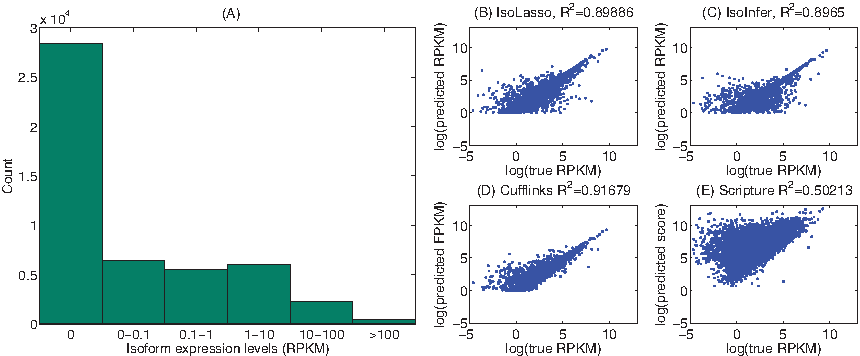
The distribution of the expression levels of all 49409 isoforms in the UCSC mm9 gene annotation is plotted in Figure 2A.

FIG. 2.

The distribution of simulated isoform expression levels (A), and the expression level estimation accuracies of IsoLasso (B), IsoInfer without TSS/PAS (C), Cufflinks (D), and Scripture (E). Note that Scripture computes a “weighted score” instead of RPKM value for each predicted isoform.

3.1.1. Matching criteria

All assembled isoforms (referred to as “candidate isoforms”) are matched against all known isoforms in the annotation (referred to as “benchmark isoforms”). Two isoforms match iff:

1. They include the same set of exons; and

2. All internal boundary coordinates (i.e., all the exon coordinates except the beginning of the first exon and the end of the last exon) are identical.

Two single-exon isoforms match iff the overlapping area occupies at least 50% the length of each isoform.

Following (Feng et al., 2010), we use sensitivity, precision and effective sensitivity to evaluate the performance of different programs. Sensitivity and precision are defined as follows: if K out of M benchmark isoforms match K′ out of N candidate isoforms, then \documentclass{aastex}\usepackage{amsbsy}\usepackage{amsfonts}\usepackage{amssymb}\usepackage{bm}\usepackage{mathrsfs}\usepackage{pifont}\usepackage{stmaryrd}\usepackage{textcomp}\usepackage{portland,xspace}\usepackage{amsmath,amsxtra}\pagestyle{empty}\DeclareMathSizes{10}{9}{7}{6}\begin{document}\begin{align*} { \rm sensitivity} & = K / M \tag{10} \end{align*}\end{document} \documentclass{aastex}\usepackage{amsbsy}\usepackage{amsfonts}\usepackage{amssymb}\usepackage{bm}\usepackage{mathrsfs}\usepackage{pifont}\usepackage{stmaryrd}\usepackage{textcomp}\usepackage{portland,xspace}\usepackage{amsmath,amsxtra}\pagestyle{empty}\DeclareMathSizes{10}{9}{7}{6}\begin{document}\begin{align*} { \rm precision } &= K^{ \prime} / N \tag{11} \end{align*}\end{document}

Note that several candidate isoforms may match the same benchmark isoform.

Effective sensitivity is calculated based on the isoforms satisfying Condition I defined in Feng et al. (2010). Isoforms satisfying Condition I are those with all segment junctions covered by at least one short read. If there are S benchmark isoforms satisfying Condition I and K of them are matched, then \documentclass{aastex}\usepackage{amsbsy}\usepackage{amsfonts}\usepackage{amssymb}\usepackage{bm}\usepackage{mathrsfs}\usepackage{pifont}\usepackage{stmaryrd}\usepackage{textcomp}\usepackage{portland,xspace}\usepackage{amsmath,amsxtra}\pagestyle{empty}\DeclareMathSizes{10}{9}{7}{6}\begin{document}\begin{align*} { \rm effective \ sensitivity} = K / S \tag{12} \end{align*}\end{document}

Intuitively, isoforms satisfying Condition I are those that are relatively easy to predict, since all their segment junctions are covered by short reads. It is shown in Feng et al. (2010) that an isoform with a higher expression level is more likely to satisfy this condition.

3.2. Comparisons between IsoLasso, IsoInfer, Cufflinks, and Scripture

3.2.1. Sensitivity, precision, and effective sensitivity

In this section, we use the sensitivity, precision and effective sensitivity defined above to compare IsoLasso with the most recent versions of IsoInfer (version V0.9.1, downloaded from www.cs.ucr.edu/∼jianxing/IsoInfer.html), Cufflinks (version 0.9.1, downloaded from website http://cufflinks.cbcb.umd.edu), and Scripture (beta version, downloaded from www.broadinstitute.org/software/scripture/home). We use TopHat (Trapnell et al., 2009) to map all simulated short reads with multi-reads discarded. Then, the read mapping information serves as the input for all four programs. Since IsoInfer is based on the assumption that the boundaries of all genes and exons are known, we infer exon boundaries from mapped junction reads using TopHat and infer gene boundaries by clustering overlapping mapped reads. Note that IsoInfer is actually designed to take advantage of any known transcription start site and poly-A site (TSS/PAS) information, although it also works without such information. Since the other three programs do not use the TSS/PAS information, neither does IsoInfer use such information in the comparison.

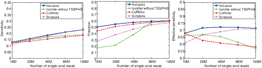
Figures 3 and 4 plot the sensitivity, precision, and effective sensitivity using various numbers of single-end and paired-end reads, respectively. On single-end reads, all transcriptome assembly tools achieve a higher sensitivity and precision as more reads are used for the assembly. Among them, IsoLasso outperforms all other programs with respect to all three criteria. This is perhaps because IsoLasso is able to maintain a good interpretation by filtering out many lowly expressed false predictions (which leads to a high precision), while keeping highly expressed isoforms and a high effective sensitivity. Scripture seems to benefit the most when more reads are available. Also, IsoInfer exhibits a sharp increase in precision from less than 20% to more than 50%, at the cost of decreased effective sensitivity (by about 10%).

FIG. 3.

Sensitivity (left), precision (middle), and effective sensitivity (right) on single-end reads.

FIG. 4.

Sensitivity (left), precision (middle), and effective sensitivity (right) on paired-end reads.

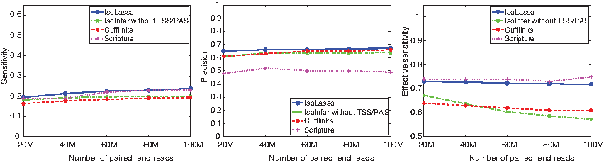
On paired-end reads, IsoLasso also achieves the best precision and sensitivity as well as a good balance between precision and effective sensitivity. However, it is surprising to see that when the number of paired-end reads increases from 20M to 100M, a less than 10% increase in sensitivity and precision is observed for all the algorithms. Also, none of the algorithms have a significant increase in effective sensitivity. In fact, both Cufflinks and IsoInfer see their effective sensitivities decreased a bit when more single-end and paired-end reads are used. This is because more benchmark isoforms would satisfy Condition I of Feng et al. (2010) as the sequencing depth increases. In this case, more isoforms are expected to be expressed for each gene, which result in a more complicated overlap graph for Cufflinks and a larger search space for IsoInfer.

Cufflinks reaches a high precision by filtering out many lowly expressed isoforms, but this sacrifices the effective sensitivity. On the other hand, Scripture achieves the highest effective sensitivity by enumerating all possible paths in the connectivity graph, but its precision is low since many of the paths are false positives.

3.2.2. Expression level estimation

All programs estimate the expression levels of predicted isoforms using different measures. Both IsoLasso and IsoInfer estimate expression levels in RPKM (Mortazavi et al., 2008), while Cufflinks uses the term FPKM (expected number of Fragments Per Kilobase of transcript sequence per Millions base pairs sequenced) (Trapnell et al., 2010). Scripture does not predict expression levels directly; instead, it computes a “weighted score” for each isoform to indicate how likely the isoform is expressed.

Figure 2B–E plots the predicted and true expression levels for all predicted isoforms which are matched to the benchmark isoforms and have expression levels >1 RPKM, using the 80M paired-end read dataset. The plots show that IsoLasso, IsoInfer and Cufflinks estimate expression levels quite accurately (the squared correlation coefficient between the predicted and true expression levels is R² > 0.89), while the “weighted score” of Scripture does not directly reflect the true expression level of isoforms (R² = 0.50). Cufflinks shows the highest prediction accuracy in expression level estimation (R² = 0.91) partly because it uses an accurate iterative statistical model to estimate the expression levels (Trapnell et al., 2010), which could potentially be incorporated into our method as a refinement step.

3.2.3. More isoforms, more difficult to predict

Intuitively, genes with more isoforms are more difficult to predict. We group all the genes by their numbers of isoforms, and calculate the sensitivity and effective sensitivity of the algorithms on genes with a certain number of isoforms as shown in Figure 5 (middle and right). Figure 5 (left) shows the total number of isoforms and isoforms satisfying Condition I (Feng et al., 2010) grouped by the number of isoforms per gene.

FIG. 5.

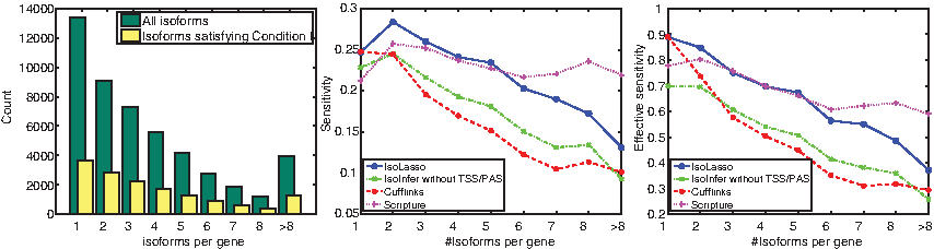
The total number of isoforms and isoforms satisfying Condition I (left), and the sensitivity (middle) and effective sensitivity (right) of the algorithms grouped by the number of isoforms per gene. Here, 100M paired-end reads are simulated.

Figure 5 shows that genes with more isoforms are more difficult to predict correctly, as both sensitivity and effective sensitivity decrease for genes with more isoforms. IsoLasso and Scripture outperform IsoInfer and Cufflinks in general. IsoLasso has a higher sensitivity and effective sensitivity on genes with at most 5 isoforms, but Scripture catches up with IsoLasso on genes containing more than 5 isoforms.

3.2.4. Running time

Figure 6 plots the running time of all four transcript assembly programs using various numbers of paired-end reads. The time for data preparation is excluded, including mapping reads to the reference genome and preparing required input files for both IsoLasso and IsoInfer. Surprisingly, although employing a search algorithm, IsoInfer runs much faster than that of any other algorithm. This is partly due to the heuristic restrictions that IsoInfer adopts to reduce the search space (e.g., requiring the candidate isoforms to satisfy Condition I and some other conditions), and the programming languages used in each tool (IsoInfer, IsoLasso, Scripture, and Cufflinks use C++, Matlab, Java, and Boost C++, respectively). All programs are run on a single 2.6-GHz CPU, but Cufflinks allows the user to run on multiple threads, which may substantially speed up the assembly process.

FIG. 6.

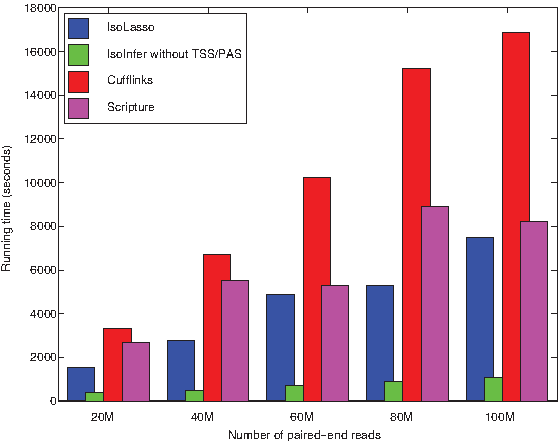
The running time for all the algorithms.

3.3. Real RNA-Seq data

Reads from two real RNA-Seq experiments are used to evaluate the performance of IsoLasso, Cufflinks and Scripture. We exclude IsoInfer from the comparison because its algorithm is similar to (and improved by, as seen from the simulation results) the algorithm of IsoLasso. One RNA-Seq read dataset is generated from the C2C12 mouse myoblast cell line (NCBI SRA accession number SRR037947 [Trapnell et al., 2010]), and the other from human embryonic stem cells (Caltech RNA-Seq track from the ENCODE project [The ENCODE Project Consortium, 2007]; NCBI SRA accession number SRR065504). Both RNA-Seq datasets include 70 million and 50 million 75-bp paired-end reads which are mapped to the UCSC mus musculus (mm9) and homo sapiens (hg19) reference genomes using Tophat (Trapnell et al., 2009), respectively.

Isoforms inferred by programs IsoLasso, Cufflinks, and Scripture are first matched against the known isoforms from mm9 and hg19 reference genomes. There are a total of 11484 and 12193 known mouse and human isoforms recovered by at least one program, respectively (Fig. 7A, B). Among these isoforms, 4485 (39%) and 4274 (35%) isoforms are detected by all programs, while 8204 (71%) and 8084 (66%) isoforms are detected by at least two programs. These numbers show that, although there is a large overlap (more than 60%) among the known isoforms recovered by these programs, each program also identifies a substantially large number of “unique” isoforms. Such “uniqueness” of each program is shown more clearly if we compute the overlap between their predicted isoforms directly (Fig. 7C, D). Each of the three programs predicts more than 40,000 isoforms on both dataset, but only shares 2–20% isoforms with other programs. About 49.5% of the mouse isoforms (46% in human) inferred by IsoLasso are also predicted by at least one of other two programs, which is substantially higher than Cufflinks (27.7% in mouse and 38.4% in human) and Scripture (4.6% in mouse and 7.4% in human). This may indicate that IsoLasso's prediction is more reliable than those of Cufflinks and Scripture since it receives more support from other (independent) programs.

FIG. 7.

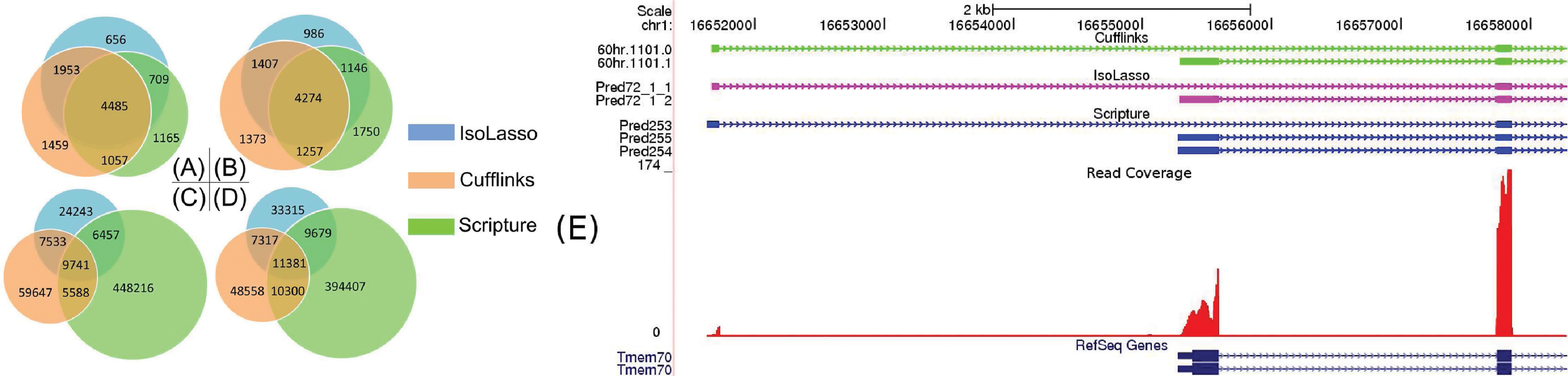
The numbers of matched known isoforms of mouse (A) and human (B), and the numbers of predicted isoforms of mouse (C) and human (D), assembled by IsoLasso, Cufflinks and Scripture. (E) An alternative 5″ start isoform of gene Tmem70 in mouse C2C12 myoblast RNA-Seq data (Trapnell et al., 2010). This isoform does not appear among the known isoforms, but is detected by IsoLasso, Cufflinks, and Scripture. Tracks from top to bottom: Cufflinks predictions, IsoLasso predictions, Scripture predictions, the read coverage, and the Tmem70 gene in the mm9 RefSeq annotation.

Note that among all the isoforms inferred by IsoLasso, Cufflinks, and Scripture, 9741 mouse isoforms and 11381 human isoforms are predicted by all three programs. These isoforms could be considered as “high-quality” ones. However, fewer than a half of these “high-quality” isoforms (4485 in mouse and 4274 in human) could be matched to the known mouse and human isoforms (Fig. 7A, B). This suggests that the current genome annotations of both mouse and human are still incomplete. An example of the “high-quality” isoforms is shown in Figure 7E. Here, an isoform with an alternative 5′ end of gene Tmem70 in mouse is predicted by all three programs but cannot be found in the mm9 RefSeq annotation or GenBank mRNAs (track not shown in the figure).

4. Conclusion

RNA-Seq transcriptome assembly is a challenging computational biology problem that arises from the development of second generation sequencing. In this article, we proposed three fundamental objectives/principles in the transcriptome assembly: prediction accuracy, interpretation, and completeness. We also presented IsoLasso, an algorithm based on the LASSO approach that seeks a balance between these objectives. Experiments on simulated and real RNA-Seq datasets show that, compared with the existing transcript assembly tools (IsoInfer, Cufflinks, and Scripture), IsoLasso is efficient and achieves the best overall performances in terms of sensitivity, precision, and effective sensitivity.

Footnotes

Acknowledgments

IsoLasso is available at . We thank the anonymous referees for many constructive comments. The research is supported in part by the NSF (grant IIS-0711129) and the NIH (grant AI078885).

Disclosure Statement

No competing financial interests exist.

References

K.F.

, Jiang

, Lin

et al. 2010. Detection of splice junctions from paired-end RNA-Seq data by splicemap. Nucleic Acids Res., 38:4570–4578.

Birol

, Jackman

S.D.

, Nielsen

C.B.

et al. 2009. De novo transcriptome assembly with abyss. Bioinformatics, 25:2872–2877.

Cloonan

, Forrest

A.R.R.

, Kolle

et al. 2008. Stem cell transcriptome profiling via massive-scale mRNA sequencing. Nat. Meth., 5:613–619.

Efron

, Hastie

, Johnstone

et al. 2004. Least angle regression. Ann. Stat., 32:407–499.

Feng

, Li

, Jiang

2010. Inference of isoforms from short sequence reads. Lect. Notes Comput Sci., 6044:138–157.

Gustafsson

, Hornquist

, Lombardi

2005. Constructing and analyzing a large-scale gene-to-gene regulatory network-LASSO-constrained inference and biological validation. IEEE/ACM Trans. Comput. Biol. Bioinform., 2:254–261.

Guttman

, Garber

, Levin

J.Z.

et al. 2010. Ab initio reconstruction of cell type-specific transcriptomes in mouse reveals the conserved multi-exonic structure of lincRNAs. Nat. Biotech., 28:503–510.

Haas

B.J.

, Zody

M.C.

2010. Advancing RNA-Seq analysis. Nat. Biotech., 28:421–423.

Hastie

, Tibshirani

, Friedman

J.H.

2009. The Elements of Statistical Learning: Data Mining, Inference, and Prediction. Springer: New York.

10.

Hocking

R.R.

, Leslie

R.N.

1967. Selection of the best subset in regression analysis. Technometrics, 9:531–540.

11.

Hoerl

A.E.

, Kennard

R.W.

1970. Ridge regression: biased estimation for nonorthogonal problems. Technometrics, 12:55–67.

12.

Holt

K.E.

, Parkhill

, Mazzoni

C.J.

et al. 2008. High-throughput sequencing provides insights into genome variation and evolution in Salmonella typhi. Nat. Genet., 40:987–993.

13.

Jiang

, Wong

W.H.

2009. Statistical inferences for isoform expression in RNA-Seq. Bioinformatics, 25:1026–1032.

14.

Kim

, Sohn

K.-A.

, Xing

E.P.

2009. A multivariate regression approach to association analysis of a quantitative trait network. Bioinformatics, 25:i204–i212.

15.

Lee

, Seo

C.H.

, Lim

et al. 2010. Accurate quantification of transcriptome from RNA-Seq data by effective length normalization. Nucleic Acids Res., 39:e9.

16.

, Jiang

, Wong

W.H.

2010. Modeling non-uniformity in short-read rates in RNA-Seq data. Genome Biol., 11:R50.

17.

Lister

, O'Malley

R.C.

, Tonti-Filippini

et al. 2008. Highly integrated single-base resolution maps of the epigenome in Arabidopsis. Cell, 133:523–536.

18.

, Song

, Huang

2007. Supervised group LASSO with applications to microarray data analysis. BMC Bioinform., 8:60.

19.

Marioni

J.C.

, Mane

S.M.

et al. 2008. RNA-Seq: an assessment of technical reproducibility and comparison with gene expression arrays. Genome Res., 18:1509–1517.

20.

Morin

, Bainbridge

, Fejes

et al. 2008. Profiling the HeLa s3 transcriptome using randomly primed cDNA and massively parallel short-read sequencing. BioTechniques, 45:81–94.

21.

Morozova

, Hirst

, Marra

M.A.

2009. Applications of new sequencing technologies for transcriptome analysis. Annu. Rev. Genomics Hum. Genet., 10:135–151.

22.

Mortazavi

, Williams

B.A.

, McCue

et al. 2008. Mapping and quantifying mammalian transcriptomes by RNA-Seq. Nat. Meth., 5:621–628.

23.

Nagalakshmi

, Wang

, Waern

et al. 2008. The transcriptional landscape of the yeast genome defined by RNA sequencing. Science, 320:1344–1349.

24.

Paşaniuc

, Zaitlen

, Halperin

2010. Accurate estimation of expression levels of homologous genes in RNA-Seq experiments. Lect. Notes Comput. Sci., 6044:397–409.

25.

Park

M.Y.

, Hastie

2007. L1-regularization path algorithm for generalized linear models. J. R. Stat. Soc. Ser. B Stat. Methodol., 69:659–677.

26.

Richard

, Schulz

M.H.

, Sultan

et al. 2010. Prediction of alternative isoforms from exon expression levels in RNA-Seq experiments. Nucleic Acids Res., 38:e112.

27.

Sammeth

, Lacroix

, Ribeca

et al. 2010. The flux simulator. Available at: http://flux.sammeth.net. Accessed August, 15:2011.

28.

Srivastava

, Chen

2010. A two-parameter generalized Poisson model to improve the analysis of RNA-Seq data. Nucleic Acids Res., 38:e170.

29.

The ENCODE Project Consortium. 2007. Identification and analysis of functional elements in 1% of the human genome by the ENCODE pilot project. Nature, 447:799–816.

30.

The Mathworks. 2004. Optimization Toolbox User's Guide. The Mathworks: Natick, MA.

31.

Tibshirani

1996. Regression shrinkage and selection via the LASSO. J. R. Stat. Soc. Ser. B Stat. Methodol., 58:267–288.

32.

Trapnell

, Pachter

, Salzberg

S.L.

2009. Tophat: discovering splice junctions with RNA-Seq. Bioinformatics, 25:1105–1111.

33.

Trapnell

, Williams

B.A.

, Pertea

et al. 2010. Transcript assembly and quantification by RNA-Seq reveals unannotated transcripts and isoform switching during cell differentiation. Nat. Biotech., 28:511–515.

34.

Wall

P.K.

, Leebens-Mack

, Chanderbali

et al. 2009. Comparison of next generation sequencing technologies for transcriptome characterization. BMC Genomics, 10:347.

35.

Wang

, Gerstein

, Snyder

2009. RNA-Seq: a revolutionary tool for transcriptomics. Nat. Rev. Genet., 10:57–63.

36.

Wheeler

D.A.

, Srinivasan

, Egholm

et al. 2008. The complete genome of an individual by massively parallel DNA sequencing. Nature, 452:872–876.

37.

Wilhelm

B.T.

, Marguerat

, Stephen

et al. 2008. Dynamic repertoire of a eukaryotic transcriptome surveyed at single-nucleotide resolution. Nature, 453:1239–1243.

38.

T.T.

, Chen

Y.F.

, Hastie

et al. 2009. Genome-wide association analysis by LASSO penalized logistic regression. Bioinformatics, 25:714–721.

39.

Yassour

, Kaplan

, Fraser

H.B.

et al. 2009. Ab initio construction of a eukaryotic transcriptome by massively parallel mRNA sequencing. Proc. Natl. Acad. Sci. USA, 106:3264–3269.

40.

Zou

, Hastie

2005. Regularization and variable selection via the elastic net. J. R. Stat. Soc. Ser. B Stat. Methodol., 67:301–320.