Nonparametric Combinatorial Sequence Models

1. Introduction

Proteins and nucleic acids, polymers whose primary structure can be described by a linear sequence of letters, are found in nature in an astounding diversity. Understanding the diversity of biological sequences has been a major topic in computational biology. Through inheritance and close functional coupling the nearby sequence positions in a family of biological sequences are often at a linkage disequilibrium (i.e., the letters at nearby sites tend to covary). However, in their folded form these molecules also have secondary, tertiary, and quaternary structure, which may reveal geometric proximity, and provide a basis for potential interactions of residues at distant sequence sites and even across different molecules. This creates significant difficulties in modeling diversity of certain families of sequences, where both the nearby and distant sequence positions may exhibit patterns of covariation. This difficulty is exacerbated by the fact that with only a limited number of sequences available for analysis we could arrive at multiple diversity models which are almost equally well supported by data.

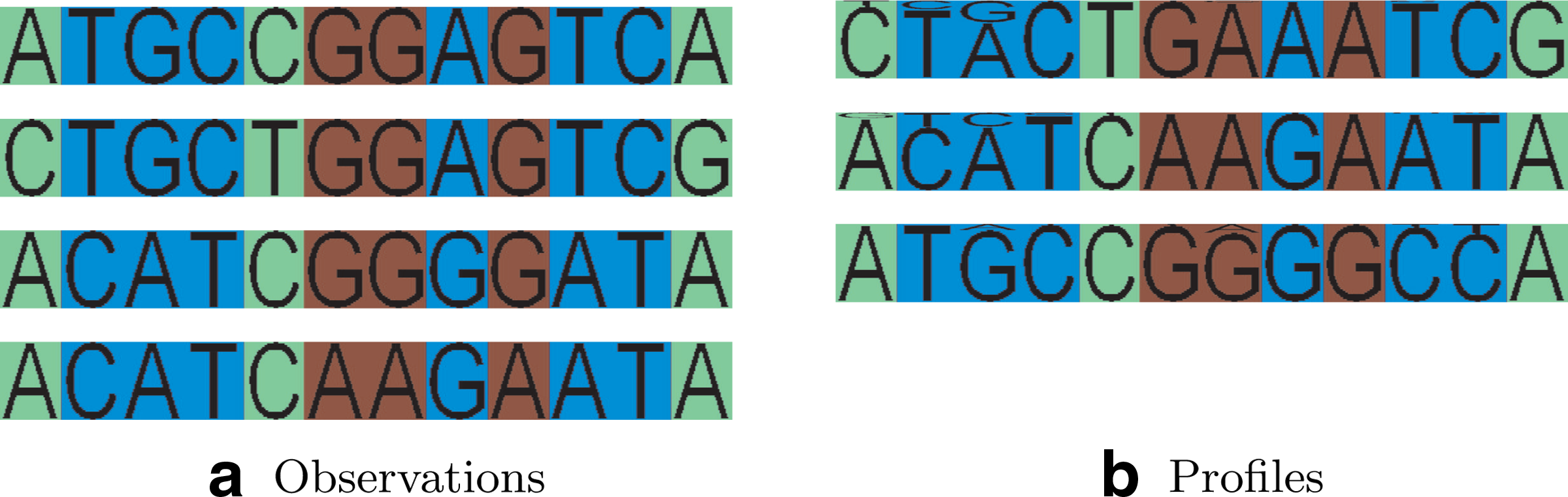
We model such sequence data starting with a basic componential strategy outlined in Figure 1. We show four aligned subsequences from Influenza HA1 genes whose diversity is well explained by first partitioning the sites into three groups and then representing each partition's induced subsequences by one of several prototypes. The site groupings do not need to follow linear patterns, and distant sites may be grouped together. Assuming that the three types in the three groups can be arbitrarily mixed, the model represents 27 different variants, and could thus also be expressed as a mixture with equally many mixture components. However, the use of a traditional mixture model would require considerably more data for training, as having obtained only 50–100 sequences it is likely that we did not see all 27 combinations. On the other hand, in a componential model it is likely that we observed all three types in all three groups multiple times, thus facilitating parameter estimation. Furthermore, the componential structure itself may be of importance. If, for instance, a phenotype of interest is linked only to one variant of one of the groups, then the mixture model would capture this variant in the nine mixture components needed to represent the relevant type in combination with three types in each of the other two site groups. Thus, traditional clustering would lead to nine different statistical tests, lowering statistical power by an order of magnitude. In this sense, a coponential structure allows for pooling of the traditional mixture components based on the finer-grained patterns of covariation. In this paper we outline a probabilistic model that can be used to discover such structure in several gene and protein families while coping with the dearth of sequence data and the possible additional correlations among the groups. Such combinatorial diversity is ubiquitous at larger scales such as entire chromosomes. However, some very important biomolecules have relatively short segments that are under significant diversifying selection. In Table 1, we highlight molecules involved in host-pathogen interactions and whose subsequences fit the model discussed above. All these families of molecules have to maintain their biological function while exhibiting a high degree of variation concentrated in a short subsequence, and the solution to these conflicting requirements has componential structure.

OPEN IN VIEWER

FIG. 1.

(a) Four aligned short subsections of the sequences exhibiting the combinatorial pattern according to the partition highlighted by color. The blue component, z_site = 1, comes in two variants, TGCATC and CATGAT, while the green component, z_site = 2, follows either ACA or CTG. All four combinations of types of these segments are found in the data. Each of those configurations can be combined with two further variants, GGG and AAA, in the red component, z_site = 3. (b) Slight perturbations on the basic types are possible as captured by the profiles inferred whose appropriate sections are shown. The profiles and subsequences correspond to appropriate sections of the Influenza HA1 genes analyzed in Section 4. The sequence sites switch among profiles in groups—the entire component follows one of the three profiles. (In general, some components may be less entropic than others and the sequences may then not be mapped to all three different types.) The four sequences in this example can be represented by the pointers z_prof for each of the three components which map the components to the appropriate profiles: 213, 113, 223, and 222. Such compression of the variability can increase statistical power of techniques mapping genotypic and phenotypic variation as we demonstrate for the case of MHC binding prediction in Section 4.

As the first example, we point to the genes encoding immunoglobulin and T cell receptor proteins which are split into multiple gene segments in the germline. These segments are made contiguous through recombination in somatic tissues by the well known V(D)J recombination process (Fugmann et al., 2000). To assemble an antigen receptor gene, one V (variable), one J (joining) and, sometimes, one D (diversity) segment are joined to create an exon that encodes the binding portion of the receptor chain. As there are typically many V, D, and J gene segments, V(D)J recombination creates an immense combinatorial diversity of antibody and TCR binding specificities, responding to the diversity of the immune system's targets.

Pathogen proteins whose subsequences are often targets of immunoglobulin and TCR binding also exhibit combinatorial diversity. For instance, VAR2CSA, a member of the P. falciparum erythrocyte membrane 1 protein family and a potential vaccine candidate for pregnancy-associated malaria, contains short segments in which the isolate variation can be well summarized by a small number of very different types. While human-infecting P. falciparum isolates exhibit combinatorial diversity resulting from fairly arbitrary mixing of segment types, each type is remarkably conserved across isolates that have them, including isolates of P. reichenowi which infects other primates (Bockhorst et al., 2007). This indicates a possible role of recombination with other var gene segments in creating combinatorial diversity in the binding domains of these proteins, which have to facilitate adhesion to the placenta while avoiding recognition by the immune system.

The third example we highlight is the major histocompatibility complex (MHC) class I family of molecules which again participate in the interaction between the host immune system and pathogens. In virtually all cells of higher organisms, these molecules present antigenic cellular peptides on the cellular surface for surveillance by cytotoxic T cells. The T cell receptor proteins discussed above may bind to the complex made of the MHC molecule and the antigenic peptide which can lead to the destruction of the infected cell. To properly facilitate the surveillance of the cellular proteome, MHC molecules are again faced with complex requirements: Across different situations, the MHC molecules will encounter a large number of different targets that may need to be carried to the surface, but at any given time, the cellular presentation should be limited to useful targets. Furthermore, as pathogens adapt to immune pressure quickly, a population of hosts is more resilient if it is diverse in its immune surveillance properties. Nature's solution here is somewhat different than in the case of the TCR and immunoglobulin. The immune system needs to learn to tolerate normal self proteins and the variation in binding properties through clonal recombination in one individual would complicate this tolerance. Instead, in humans three highly diverse loci encode for MHC class I, leading to diversity of MHC binding specificities across individuals, not within one host. The residues forming the peptide binding groove of the MHC molecules have been found to be under a diversifying selection. The statistical study of MHC alleles has yielded evidence of both large-scale recombination events (involving entire exons) and low-scale recombination events (involving apparent exchange of short DNA segments), but convergent evolution in parts of the MHC from different alleles is also supported by the data (Hughes et al., 1993). Thus, a variety of mutation and recombination events, whose combinations were selected based on the resulting binding properties of the MHC groove lead to the immense diversity at this locus, the most polymorphic in the human genome.

In these three examples, and many more (Figure 1 illustrates diversity in an influenza protein), the functional requirements have created sequence families that exhibit high levels of diversity with combinatorial structure similar to the one illustrated in Figure 1. Models that capture such structure have immediate applications in low-level tasks such as sequencing, haplotype recovery, as well as in higher level tasks involving the matching of the genetic diversity to phenotypic variation. In the case of the immunoglobulin, this structure is essentially encoded in the human genome, and the different V, D, and J variants can be directly read off there. But, when diversity is maintained on a population level, as is the case with most pathogen proteins and RNA molecules, as well as MHC or KIR (receptor on natural killer cells) among human proteins, then we can only recover the structure by analyzing sequences from a number of individuals. This is complicated by two effects: first, the illustration in Figure 1 is a simplification. The groups of sites are only approximately independent of each other. Some residual weak linkage is expected to exist even in the case of the optimal sequence partition. Secondly, due to the high polymorphism in the families of interest the structure in Figure 1 can only be estimated reliably when sufficient data is available. When data is scarce, multiple solutions are possible that differ little in the data fit.

In this paper we propose a model that differs from existing models in the way it addresses these two issues. In Bockhorst and Jojic (2007) and Bockhorst et al. (2007), the partition is assumed to consist of contiguous segments, a constraint that does not hold for many interesting diversity patterns (cf. Fig. 1), and a single optimal segmentation (cf. the pattern library/epitome approach of Jojic et al. [2004, 2006]). A combinatorial optimization algorithm for site clustering that does not promote contiguous segments is proposed in Narasimhan et al. (2006), but, as the basic generative model creates blocks with limited diversity (Jojic and Caspi, 2004; Jojic et al., 2004), the result is again a single optimal segmentation which can be sensitive to the size of the sequence set used to estimate it.

We propose a Bayesian hierarchical site clustering approach with a minimal number of parameters which not only captures weak linkage among components at the first level of the clustering hierarchy, but also naturally adjusts to the size of the dataset. Furthermore, we develop a sampling procedure that produces an estimate of the posterior over possible sequence partitions. In Section 4, we illustrate for three families of proteins—MHC class I, Influenza HA1 and KIR—that the componential model discussed here is a better fit than traditional mixture models, which cluster entire sequences (phylogenetic methods fall in this category). We also show an example where by using the distribution over multiple partitions we improve on the ability to match the genetic diversity with the phenotypic variation.

In particular, by representing MHC sequences using the latent variables in our model, we train simple MHC class I–peptide binding estimators. We show that by integrating over possible MHC sequence representations we obtain better predictions than when using the latent variables for the MAP estimate of the segmentation structure.

Matlab code for the sequence model can be found at http://cs.berkeley.edu/~flw/ncsm and http://research.microsoft.com/∼jojic/ncsm.

2. Model

Most approaches to capturing diversity in sets of aligned sequences treat each sequence as a whole, applying clustering techniques (e.g., neighbor-joining or maximum likelihood approaches) or building a hierarchical clustering of sequences (e.g., a phylogenetic tree). A special case of such approaches are mixture models which describe aligned sequences as being sampled from a mixture of a small number of “latent profiles,” also known as “position-specific scoring matrices” (PSSMs) (King and Roth, 2003). As outlined above, a considerable drawback of a whole-sequence mixture model is that each observed sequence corresponds in its entirety to one latent profile, which in turn can diminish the quality of inferred parameters. Our model is a generalized mixture model that relaxes this constraint and allows different sequence positions to correspond to different profiles. To retain some structure, however, our model introduces a latent partitioning that groups site positions into linked sites that must be sampled from the same profile. Each such “site group” thus induces a different mixture model on its component sites. This allows us to capture combinatorial diversity that is not discribed well by flat mixture models—n site groups with k profiles each would need n^k mixture components if the data was to be represented by a flat mixture. Moreover, as discussed in Section 1, we wish to also couple the mixture models in order to capture additional weaker links among the site groups. Our model achieves this by implicitly coupling the mixing proportions of the different mixtures.

When analyzing data with traditional mixture models, one is faced with the perennial problem of choosing the number of mixture components. Since the model we are proposing can be thought of as a refined mixture model, it is not immune to this issue. While information-theoretic techniques do exist for estimating the structural parameters in mixture models, they are difficult to justify when the number of components required to represent a dataset is large (Xing et al., 2006). In a number of biological applications (Qin, 2006; Ting et al., 2010; Xing et al., 2004, 2006) nonparametric methods based on the Chinese restaurant process (CRP), or the closely related Dirichlet process, have been shown to elegantly circumvent such issues by effectively introducing a prior distribution on the number of latent components. Additionally, the induced prior automatically accommodates more latent components as the amount of data grows. This allows us to infer conservative representations with few components when little data is available while being flexible enough to represent complex patterns emerging from larger datasets.

Our model relies on a composition of two nonparametric priors—the Chinese restaurant process (CRP) (Pitman, 2002) and the related Chinese restaurant franchise (CRF) (Teh et al., 2006). By incorporating these two nonparametric priors we avoid fixing the number of site groups and the number of profile variants a priori. To make predictions, we will average over these choices under the induced posterior distribution.

In this section, we present our model by means of a sequential, generative description. We will use the variable s to index sequences and i to index sites (positions) within a sequence. Let M denote an S × I matrix of aligned sequences, so that m_s denotes the s-th sequence and m_s,i denotes the i-th symbol in the s-th sequence. Our model relies on four sets of latent random variables: z_site, z_seq, z_prof and θ, sampled in top-down fashion according to a CRF that is conditioned on a partition sampled from a CRP.

2.2. Chinese restaurant franchise observation model

The second part of our model represents a combinatorial observation model over aligned sequences in the form of a CRF (Teh et al., 2006) that is conditioned on the initial partitioning z_site by the CRP. The CRF is a generalization of the CRP to allow multiple parallel restaurants to share parameters. Specifically, where in the CRP each table is given a parameter which is shared among its occupants, in the CRF these parameters can also be shared across multiple CRPs. It will turn out that the “parameters” that are being shared in our application are pointers to profiles, rather than the profiles themselves. As such, our model can be thought of as an instance of a dependent nonparametric process, discussed by MacEachern (1999), where individual parameters are replaced by stochastic processes.

Sampling secondary site linkages

In the CRF we interpret each observed sequence as its own restaurant. Instead of thinking of site positions as customers, as in a standard application of the CRF, we now consider the previously induced site groups to be customers. Each restaurant is visited by all site groups, so that the union of the site groups at each restaurant captures the entire set of sequence indices. The CRF is defined as follows. At each sequence m_s the n_site site groups indicated in z_site are seated at tables a second time according to the rules of a CRP. The seating arrangement of the site groups is represented by latent variables \documentclass{aastex}\usepackage{amsbsy}\usepackage{amsfonts}\usepackage{amssymb}\usepackage{bm}\usepackage{mathrsfs}\usepackage{pifont}\usepackage{stmaryrd}\usepackage{textcomp}\usepackage{portland, xspace}\usepackage{amsmath, amsxtra}\pagestyle{empty}\DeclareMathSizes{10}{9}{7}{6}\begin{document} $$z_{\rm seq} (s, t), t = 1, \ldots, n_{\rm site}$$ \end{document} . Denote by n_seq (s) the number of (second-level) tables formed at sequence s at each step of the process, and let \documentclass{aastex}\usepackage{amsbsy}\usepackage{amsfonts}\usepackage{amssymb}\usepackage{bm}\usepackage{mathrsfs}\usepackage{pifont}\usepackage{stmaryrd}\usepackage{textcomp}\usepackage{portland, xspace}\usepackage{amsmath, amsxtra}\pagestyle{empty}\DeclareMathSizes{10}{9}{7}{6}\begin{document} $$c_{\rm seq} (s, u), u = 1, \ldots, n_{\rm seq} (s)$$ \end{document} denote the number of site groups present at the table u. If we parameterize the sequential seating process at each restaurant by α_seq, then conditioned on the seating assignment of the site groups \documentclass{aastex}\usepackage{amsbsy}\usepackage{amsfonts}\usepackage{amssymb}\usepackage{bm}\usepackage{mathrsfs}\usepackage{pifont}\usepackage{stmaryrd}\usepackage{textcomp}\usepackage{portland, xspace}\usepackage{amsmath, amsxtra}\pagestyle{empty}\DeclareMathSizes{10}{9}{7}{6}\begin{document} $$1, \ldots, t - 1$$ \end{document} , the seating probabilities for group t are \documentclass{aastex}\usepackage{amsbsy}\usepackage{amsfonts}\usepackage{amssymb}\usepackage{bm}\usepackage{mathrsfs}\usepackage{pifont}\usepackage{stmaryrd}\usepackage{textcomp}\usepackage{portland, xspace}\usepackage{amsmath, amsxtra}\pagestyle{empty}\DeclareMathSizes{10}{9}{7}{6}\begin{document} \begin{align*} p (z_{\rm seq} (s, t) = u \mid z_{\rm seq} (s, 1 :t - 1)) \propto \begin{cases}c_{\rm seq} (s, u) \ {\rm if} \ u \leq n_{\rm seq} (s) \\ \alpha_{\rm seq} \qquad \ {\rm if} \ u = n_{\rm seq} (s) + 1.\end{cases} \tag{2} \end{align*} \end{document}

Sampling profile allocations

In order to produce observed sequences, the CRF model next introduces pointers to sets of parameters. Each table u in a sequence restaurant s in the CRF is assigned a latent variable z_prof(s, u), that indicates which of a set of shared parameters θ is used at table u of restaurant s. We will refer to one such shared parameter θ _p as a “sequence profile.” As before, at each step of the sequential algorithm, the variable n_prof denotes how many distinct profiles the set of z_prof variables points to. The function \documentclass{aastex}\usepackage{amsbsy}\usepackage{amsfonts}\usepackage{amssymb}\usepackage{bm}\usepackage{mathrsfs}\usepackage{pifont}\usepackage{stmaryrd}\usepackage{textcomp}\usepackage{portland, xspace}\usepackage{amsmath, amsxtra}\pagestyle{empty}\DeclareMathSizes{10}{9}{7}{6}\begin{document} $$c_{\rm prof} (p), p = 1, \ldots, n_{\rm prof}$$ \end{document} reports how many of the tables in all processed sequence restaurants picked profile p. In the sequential description of the CRF, the choice of profile made by each table is influenced by the number of other tables that have previously chosen that profile. That is, the process can be thought of as another CRP in which distinct profiles act as the tables. If we use the parameter α_prof to define this CRP, then the probability that table u in restaurant s chooses profile p, given the profile choices of all tables in restaurants \documentclass{aastex}\usepackage{amsbsy}\usepackage{amsfonts}\usepackage{amssymb}\usepackage{bm}\usepackage{mathrsfs}\usepackage{pifont}\usepackage{stmaryrd}\usepackage{textcomp}\usepackage{portland, xspace}\usepackage{amsmath, amsxtra}\pagestyle{empty}\DeclareMathSizes{10}{9}{7}{6}\begin{document} $$1, \ldots, s - 1$$ \end{document} and tables \documentclass{aastex}\usepackage{amsbsy}\usepackage{amsfonts}\usepackage{amssymb}\usepackage{bm}\usepackage{mathrsfs}\usepackage{pifont}\usepackage{stmaryrd}\usepackage{textcomp}\usepackage{portland, xspace}\usepackage{amsmath, amsxtra}\pagestyle{empty}\DeclareMathSizes{10}{9}{7}{6}\begin{document} $$1, \ldots, u - 1$$ \end{document} in restaurant s, is given by \documentclass{aastex}\usepackage{amsbsy}\usepackage{amsfonts}\usepackage{amssymb}\usepackage{bm}\usepackage{mathrsfs}\usepackage{pifont}\usepackage{stmaryrd}\usepackage{textcomp}\usepackage{portland, xspace}\usepackage{amsmath, amsxtra}\pagestyle{empty}\DeclareMathSizes{10}{9}{7}{6}\begin{document} \begin{align*} p (z_{\rm prof} (s, u) = p \mid z_{\rm prof} (1 :s - 1, \cdot), z_{\rm prof} (s, 1 :u - 1)) \propto \begin{cases}c_{\rm prof} (p) \ {\rm if} \ p \leq n_{\rm prof} \\ \alpha_{\rm prof} \quad \ {\rm if} \ p = n_{\rm prof} + 1.\end{cases} \tag{3} \end{align*} \end{document}

Sampling profile parameters

For sequences with an alphabet of size |∑|, each sequence profile \documentclass{aastex}\usepackage{amsbsy}\usepackage{amsfonts}\usepackage{amssymb}\usepackage{bm}\usepackage{mathrsfs}\usepackage{pifont}\usepackage{stmaryrd}\usepackage{textcomp}\usepackage{portland, xspace}\usepackage{amsmath, amsxtra}\pagestyle{empty}\DeclareMathSizes{10}{9}{7}{6}\begin{document} $$\theta_p, p = 1, \ldots, n_{\rm prof}$$ \end{document} is comprised of I |∑|-vectors, one for each site index. Each vector θ _p (·, i) is a probability distribution over the |∑| possible symbols that could be observed at position i. When a new table in one of the restaurants chooses a new profile θ _p which has not yet been chosen before, the profile vectors \documentclass{aastex}\usepackage{amsbsy}\usepackage{amsfonts}\usepackage{amssymb}\usepackage{bm}\usepackage{mathrsfs}\usepackage{pifont}\usepackage{stmaryrd}\usepackage{textcomp}\usepackage{portland, xspace}\usepackage{amsmath, amsxtra}\pagestyle{empty}\DeclareMathSizes{10}{9}{7}{6}\begin{document} $$\theta_p (\cdot, i), i = 1, \ldots, I$$ \end{document} are sampled from a Dirichlet prior, parameterized by α_dir.

Sampling observed sequences

Once all latent variables and profiles have been sampled, the observed sequences are generated as follows: given the latent variables z_site, z_seq, z_prof and profiles θ, we generate the symbol at position i in sequence s by sampling from a multinomial with parameter θ _p ( · , i), where \documentclass{aastex}\usepackage{amsbsy}\usepackage{amsfonts}\usepackage{amssymb}\usepackage{bm}\usepackage{mathrsfs}\usepackage{pifont}\usepackage{stmaryrd}\usepackage{textcomp}\usepackage{portland, xspace}\usepackage{amsmath, amsxtra}\pagestyle{empty}\DeclareMathSizes{10}{9}{7}{6}\begin{document} $$p = z_{\rm prof} (s, z_{\rm seq} (s, z_{\rm site} (i)))$$ \end{document} .

The overall sequential process we have so far described is summarized in Figure 2. The sampling procedure generates data that exhibit the combinatorial structure discussed in Figure 1 and found in a variety of biological sequence families. Of course, our goal is to reverse this process. Starting from the observed sequences we need to reconstruct the latent variables z_site, z_seq, z_prof and the profile sequences, while making explicit our uncertainty over these structures. In the next section, we develop an inference algorithm that achieves this by approximating the full posterior over latent structures.

OPEN IN VIEWER

FIG. 2.

A graphical representation of the stochastic process for three aligned sequences, m₁, m₂, m₃. Tables in restaurants are indicated as circles with patrons seated around the perimeter. The initial partitioning of sequence positions (numerals) is represented by the shaded tables above the dashed line. Below the dashed line, those site groups (now indicated by small circles with matching shadings) are seated again at tables in each of the three sequence restaurants. Lastly, each table in a sequence restaurant chooses a profile (i.e., a parameter) to point to. In our implementation, each parameter is a PSSM consisting of one probability vector for each sequence position. For clarity of exposition we only show the choices for tables in the third sequence restaurant. The profile choice indirectly associates each sequence position in m₃ with one of the profiles, as indicated by the matching colorings. This association reflects both the initial sequence partitioning as well as the choice of profiles by sequence tables. The final sequence m₃ is generated by sampling each symbol from a multinomial distribution with parameter given by the corresponding probability vector of the allocated PSSM.

3. Inference

We use a collapsed Gibbs sampler in which the profiles θ are integrated out. The algorithm cycles through resampling the site grouping z_site, the secondary grouping of site groups z_seq and the assignment of profiles z_prof, at each step conditioning on all remaining latent variables. A central property of the CRP and CRF that facilitates this sampling process is exchangeability. Exchangeability allows us to treat any customer of a restaurant as if it were the last customer to enter the restaurant. This is consistent with our modeling assumption that sites have unique positions that need to be grouped, but that the ordering of these positions is of little value, since parts may be non-contiguous. The consequence of this exchangeability is that we can now easily sample an updated table seating for any customer in a restaurant. In the following we show the main computations for resampling the site grouping z_site. The posteriors for sampling updated variables z_seq and z_prof can be derived analogously to Teh et al. (2006).

4. Results

To demonstrate the versatility of our model, we applied it to three sequence datasets in which we expect combinatorial patterns to exist. In the following, we have focused our analysis on a small number of the most polymorphic sites in each dataset. The first dataset are 526 aligned amino-acid sequences of length 50 for MHC class I proteins from all three alleles A, B, C. The flu dataset comprises aligned 22-long amino-acid sequences for 255 HA1 genes in influenza strains covering the years 1968–2003. The KIR dataset are sequences of unordered (i.e., unphased) pairs of haplotype measurements at 229 SNPs. These SNPs encode variability of a killer cell immunoglobulin-like receptor. If we knew the phase, we could order each pair and turn the data into aligned sequences that could easily be analyzed as outlined before. Thus, we can extend our model to work with unphased KIR data by introducing extra latent variables z_phase that encode the phasing information for each pair. The modified algorithm iterates between sampling phasing variables to turn aligned sequences of pairs into aligned sequences, and then sampling new latent variables z_site, z_seq, as well as z_prof, as before.

We have carried out experiments to demonstrate that our model successfully isolates combinatorial structures from the data and learns a much more parsimonious sequence model that yields higher log likelihood than a comparable mixture model. For each of the datasets, we set up a combinatorial sequence model and computed posterior samples for different settings of the model parameters α_site, α_seq, α_prof, and α_dir. Each combination of parameters induces a different nonparametric prior over aligned sequences. We wish to compare the average data likelihoods assigned by the posterior combinatorial models to the likelihoods obtained from flat mixture models. To facilitate this comparison, we ensure that the mixture models we compare against have similar complexity as the nonparametric model. We estimate the complexity of a given model by measuring how many parameters it would take to represent a set of sequences in a typical posterior sample. If for example a sample with n_site site tables and n_prof profiles of length I with a symbol alphabet of size |∑| was found, we require a total of I(n_site − 1) + n_prof I(|∑| − 1) parameters as a shared representation across all sequences. The first I(n_site − 1) parameters encode which site position is allocated to which site group while the remaining account for the profile parameters. In comparison, a mixture model that links all site positions asserts that \documentclass{aastex}\usepackage{amsbsy}\usepackage{amsfonts}\usepackage{amssymb}\usepackage{bm}\usepackage{mathrsfs}\usepackage{pifont}\usepackage{stmaryrd}\usepackage{textcomp}\usepackage{portland, xspace}\usepackage{amsmath, amsxtra}\pagestyle{empty}\DeclareMathSizes{10}{9}{7}{6}\begin{document} $$n_{\rm site}^{\prime} = 1$$ \end{document} and for \documentclass{aastex}\usepackage{amsbsy}\usepackage{amsfonts}\usepackage{amssymb}\usepackage{bm}\usepackage{mathrsfs}\usepackage{pifont}\usepackage{stmaryrd}\usepackage{textcomp}\usepackage{portland, xspace}\usepackage{amsmath, amsxtra}\pagestyle{empty}\DeclareMathSizes{10}{9}{7}{6}\begin{document} $$n_{\rm prof}^{\prime}$$ \end{document} profiles requires \documentclass{aastex}\usepackage{amsbsy}\usepackage{amsfonts}\usepackage{amssymb}\usepackage{bm}\usepackage{mathrsfs}\usepackage{pifont}\usepackage{stmaryrd}\usepackage{textcomp}\usepackage{portland, xspace}\usepackage{amsmath, amsxtra}\pagestyle{empty}\DeclareMathSizes{10}{9}{7}{6}\begin{document} $$n_{\rm prof}^{\prime}I \left( \left| \sum \right| - 1\right)$$ \end{document} parameters. Assuming that a single set of such parameters is fixed, to encode a set of sequences we would need to also infer for each sequence the posterior distributions over latent variables (mixture components for the mixture model, or profile pointers z_prof in our model). Then any remaining uncertainty as to the identity of the letters in individual positions would also have to be collapsed by encoding these individual letters. Minimum Description Length (MDL) (Rissanen, 1989) prescribes techniques for making the minimum required code length for encoding all this directly dependent on the uncertainties in the data, with less uncertain pieces encoded with shorter messages, so that the total code length in bits reduces to the log₂ likelihood under the model. By adding the cost of encoding the parameters that are shared by the sequences (profiles, partitioning information), we would obtain a description length of the dataset. The cost of encoding parameters would be proportional to the number of the parameters. Similarly, for comparing model fits, statistical literature recommends the use of the Bayesian information criterion (BIC) (Schwarz, 1978) or the Akaike information criterion (AIC) which combine the log likelihood of the data with a penalty reflecting the number of free parameters. However, rather than comparing the two models by an MDL, BIC or AIC score for only one model complexity, we present a stronger argument here: it turns out that for a wide range of model complexities, the log likelihood of the data is higher under the combinatorial model than under the mixture model.

To show this, we have collected posterior samples of varying complexity by varying the model parameters α_site, α_seq, α_prof, α_dir across a broad range and collecting posterior samples from the different induced models. For each such model, we compute the average posterior log likelihood of the data across samples. Next, for a typical posterior sample of each model we compute the smallest number \documentclass{aastex}\usepackage{amsbsy}\usepackage{amsfonts}\usepackage{amssymb}\usepackage{bm}\usepackage{mathrsfs}\usepackage{pifont}\usepackage{stmaryrd}\usepackage{textcomp}\usepackage{portland, xspace}\usepackage{amsmath, amsxtra}\pagestyle{empty}\DeclareMathSizes{10}{9}{7}{6}\begin{document} $$n_{\rm prof}^{\prime}$$ \end{document} of mixture profiles that would exceed it in complexity (i.e., \documentclass{aastex}\usepackage{amsbsy}\usepackage{amsfonts}\usepackage{amssymb}\usepackage{bm}\usepackage{mathrsfs}\usepackage{pifont}\usepackage{stmaryrd}\usepackage{textcomp}\usepackage{portland, xspace}\usepackage{amsmath, amsxtra}\pagestyle{empty}\DeclareMathSizes{10}{9}{7}{6}\begin{document} $$n_{\rm prof}^{\prime}$$ \end{document} so that \documentclass{aastex}\usepackage{amsbsy}\usepackage{amsfonts}\usepackage{amssymb}\usepackage{bm}\usepackage{mathrsfs}\usepackage{pifont}\usepackage{stmaryrd}\usepackage{textcomp}\usepackage{portland, xspace}\usepackage{amsmath, amsxtra}\pagestyle{empty}\DeclareMathSizes{10}{9}{7}{6}\begin{document} $$I (n_{\rm site} - 1) + n_{\rm prof}I \left( \left| \sum \right| - 1 \right) \leq n_{\rm prof}^{\prime}I \left.\left( \left| \sum \right| - 1 \right) \right)$$ \end{document} ). 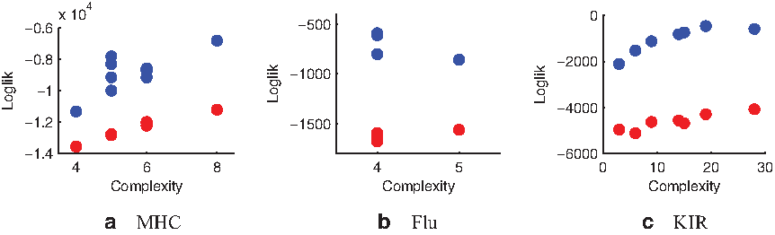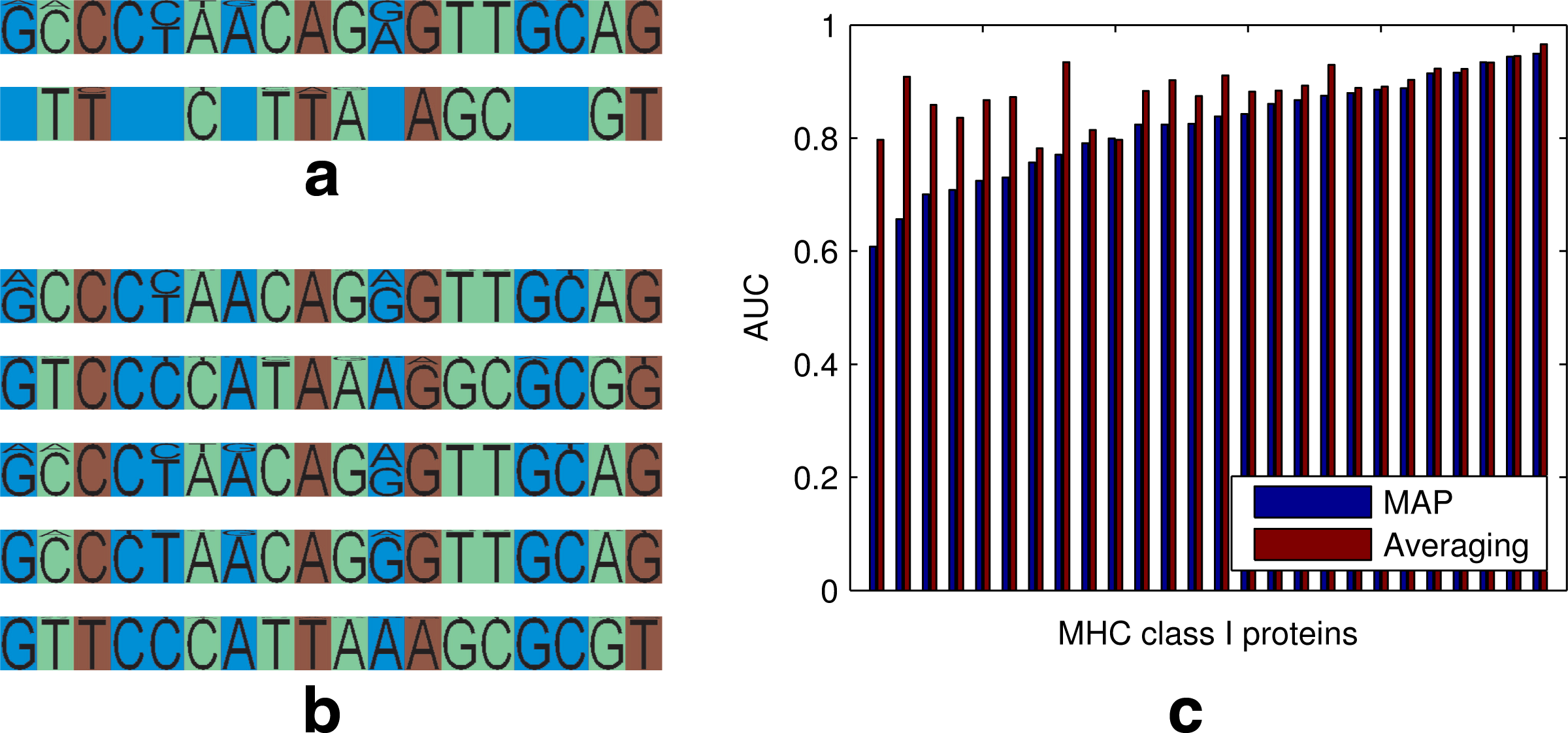We then fit five mixture models with \documentclass{aastex}\usepackage{amsbsy}\usepackage{amsfonts}\usepackage{amssymb}\usepackage{bm}\usepackage{mathrsfs}\usepackage{pifont}\usepackage{stmaryrd}\usepackage{textcomp}\usepackage{portland, xspace}\usepackage{amsmath, amsxtra}\pagestyle{empty}\DeclareMathSizes{10}{9}{7}{6}\begin{document} $$n_{\rm prof}^{\prime}$$ \end{document} profiles on the data and compute the average data log likelihood. Thus for each combination of model parameters we receive one average log likelihood under the combinatorial model and one under a matched mixture model. In Figure 3, we show for the three datasets the average log likelihood of the combinatorial model across complexities (blue scatter) as well as the average log likelihood of the matched mixture model (red scatter). For all three datasets, the log likelihood of the combinatorial model exceeds that of the mixture model considerably. Additionally, our model provides a better representation for sequence clustering. The clustering induced by our combinatorial model for Influenza HA1 sequences matches the hemagglutinin inhibition clusters of Smith et al. (2004) closer than the clusters obtained by simple mixture modeling, achieving an average adjusted rand index (Hubert and Arabie, 1985) of 0.70 versus 0.55.1 In Figure 4a, we visualize profiles as well as site groups for the first 18 SNPs of the KIR dataset for one posterior sample of the combinatorial model. Figure 4b shows relevant parts of the 5 profiles that were inferred by a simpler mixture phasing model. As can be seen, our model factorizes the profiles inferred by the simpler mixture model into a parsimonious form that can still explain the mixture variants. The green group has variants CACGTTA and TCTAGCG, while the red group follows either CAGG or TTAT. Three of the four possible combinations of these patterns occur in the profiles estimated by the mixture model. As a side effect of the compact representation, our model allows for a more careful use of data for profile parameter inference. Mixture models can capture many combinations, but they achieve this by using a substantially greater number of parameters, while still missing many of the combinations outside the region shown. This leads to significantly lower likelihood in comparison with the componential model of similar parametric complexity, as shown in Figure 3.

OPEN IN VIEWER

FIG. 3.

Comparison of the log likelihood assigned by the combinatorial model (blue scatter) with the log likelihood assigned by a mixture model of comparable complexity (red scatter) as a function of different model complexities. We show results for MHC (a), Flu (b), and KIR (c), sequences. Flu sequences require only relatively few profiles and site groups (cf. Fig. 1); thus only two model complexities were explored. To give a better intuition for the variety of posterior models captured in the scatter above, the MHC models included ones with posterior samples typically having 11–18 site groups with 2–4 profiles, and ones having 26–38 site groups with 5–7 profiles. Among the Flu models we analyzed were ones with posterior samples normally having 4–7 site groups with 3–4 profiles and ones having 8–19 site groups with 3–4 profiles. Lastly, two of the KIR models we analyzed had posterior samples with 2–4 site groups with 3–4 profiles and 59–80 site groups with 2–4 profiles.

OPEN IN VIEWER

FIG. 4.

(a) Factorized representation for the first 18 SNPs inferred by our model on the KIR data. Empty fields in the profiles denote that no further variants were found for a site group. (b) The 5 profiles for the first 18 SNPs learnt by a mixture model on KIR data. (c) AUC scores for the MHC I binding prediction task across 26 MHC proteins. Averaging regression results across posterior samples significantly improves the AUC score over using only the MAP sample to fit a regression.

5. Conclusion

This article presented a nonparametric combinatorial sequence prior that was found to be a good match for a wide range of sequence families. An important feature of the model is that it induces a posterior distribution over latent factorized representations. Our work on MHC binding prediction demonstrates that integrating out this distribution can be an important ingredient in inferences that follow the initial sequence analysis. One way to explain why averaging across predictors should be beneficial in the case of MHCs is to consider the potential for suboptimal parsing of the MHC groove. Although many MHC alleles currently present in human populations are known, we cannot directly access the extinct alleles. Thus, our estimate of the site covariation and the resulting optimal sequence partition must suffer from the limited number of sequences used to fit our model. Picking any one segmentation with a high likelihood over MHC sequences may lead to an oversimplification of the sequence representation. A posterior over the partitions, accompanied with latent variables giving sequence types in different parts, reflects more information about a set of amino acids in each MHC sequence than a latent structure based on one optimal segmentation.

References

1.
BockhorstJ., JojicN.2007. Discovering patterns in biological sequences by optimal segmentation. Proc. 23st Int. Conf. UAI.
2.
BockhorstJ., LuF., JanesJ.H.et al.2007. Structural polymorphism and diversifying selection on the pregnancy malaria vaccine candidate VAR2CSA. Mol. Biochem. Parasitol., 155:103–112.
3.
FugmannS.D., LeeA.I., ShockettP.E.et al.2000. The RAG proteins and V (D) J recombination: complexes, ends, and transposition. Ann. Rev. Immunol., 18:495–528.
4.
HubertL., ArabieP.1985. Comparing partitions. J. Classification, 2:193–218.
5.
HughesA.L., HughesM.K., WatkinsD.I.1993. Contrasting roles of interallelic recombination at the HLA-A and HLA-B loci. Genetics, 133:669–680.
6.
JojicN., CaspiY.2004. Capturing image structure with probabilistic index maps. Proc. IEEE Conf. Comput. Vision Patt. Recognit., 1:212–219.
7.
JojicN., JojicV., FreyB.et al.2006. Using “epitomes” to model genetic diversity: rational design of HIV vaccine cocktails. Adv. NIPS, 18:587–594.
8.
JojicN., JojicV., HeckermanD.2004. Joint discovery of haplotype blocks and complex trait associations from SNP sequences. Proc. 20th Int. Conf. UAI.
NielsenM., LundegaardC., WorningP.et al.2003. Reliable prediction of T-cell epitopes using neural networks with novel sequence representations. Protein Sci., 12:1007–1017.
14.
PetersB., BuiH., FrankildS.et al.2006. A community resource benchmarking predictions of peptide binding to MHC-I molecules. PLoS Comput. Biol., 2:e65.
15.
PetersB., TongW., SidneyJ.et al.2003. Examining the independent binding assumption for binding of peptide epitopes to MHC-I molecules. Bioinformatics, 1765–1772.
16.
PitmanJ.2002. Combinatorial Stochastic Processes. Springer-Verlag: New York.
17.
QinZ.S.2006. Clustering microarray gene expression data using weighted Chinese restaurant process. Bioinformatics, 22:1988–1997.
18.
RissanenJ.1989. Stochastic Complexity in Statistical Inquiry Theory. World Scientific Publishing: River Edge, NJ.
19.
SchwarzG.1978. Estimating the dimension of a model. Ann. Stat., 6:461–464.
20.
SmithD.J., LapedesA., de JongJ.C.et al.2004. Mapping the antigenetic and genetic evolution of influenza virus. Science, 305:371–376.
TingD., WangG., ShapovalovM.et al.2010. Neighbor-dependent Ramachandran probability distributions of amino acids developed from a hierarchical Dirichlet process model. PLoS Comput. Biol., 6:e1000763.
23.
XingE.P., SharanR., JordanM.I.2004. Bayesian haplotype inference via the Dirichlet process. Proc. 21st Int. Conf. Mach. Learn., 879–886.
24.
XingE.P., SohnK., JordanM.I.et al.2006. Bayesian multi-population haplotype inference via a hierarchical Dirichlet process mixture. Proc. 23rd Int. Conf. Mach. Learn., 1049–1056.