Rich Parameterization Improves RNA Structure Prediction

Abstract

Current approaches to RNA structure prediction range from physics-based methods, which rely on thousands of experimentally measured thermodynamic parameters, to machine-learning (ML) techniques. While the methods for parameter estimation are successfully shifting toward ML-based approaches, the model parameterizations so far remained fairly constant. We study the potential contribution of increasing the amount of information utilized by RNA folding prediction models to the improvement of their prediction quality. This is achieved by proposing novel models, which refine previous ones by examining more types of structural elements, and larger sequential contexts for these elements. Our proposed fine-grained models are made practical thanks to the availability of large training sets, advances in machine-learning, and recent accelerations to RNA folding algorithms. We show that the application of more detailed models indeed improves prediction quality, while the corresponding running time of the folding algorithm remains fast. An additional important outcome of this experiment is a new RNA folding prediction model (coupled with a freely available implementation), which results in a significantly higher prediction quality than that of previous models. This final model has about 70,000 free parameters, several orders of magnitude more than previous models. Being trained and tested over the same comprehensive data sets, our model achieves a score of 84% according to the F₁-measure over correctly-predicted base-pairs (i.e., 16% error rate), compared to the previously best reported score of 70% (i.e., 30% error rate). That is, the new model yields an error reduction of about 50%. Trained models and source code are available at www.cs.bgu.ac.il/∼negevcb/contextfold.

1. Introduction

Within the last few years, non-coding RNAs have been recognized as a highly abundant class of RNAs. These RNA molecules do not code for proteins, but nevertheless are functional in many biological processes, including localization, replication, translation, degradation, regulation and stabilization of biological macromolecules (Eddy, 2001; Mandal and Breaker, 2004; Washietl et al., 2005). It is generally known that much of RNAs functionalities depend on its structural features (Washietl et al., 2005; Kloc et al., 2002; Hofacker et al., 2004; Mattick, 2004). Unfortunately, although massive amounts of sequence data are continuously generated, the number of known RNA structures is still limited, since experimental methods such as NMR and Crystallography require expertise and long experimental time. Therefore, computational methods for predicting RNA structures are of significant value (Hofacker et al., 2002; Zuker, 1989, 2003). This work deals with improving the quality of computational RNA structure prediction.

RNA is typically produced as a single stranded molecule, composed as a sequence of bases of four types, denoted by the letters A, C, G, and U. In addition to the covalent bonds which are formed between adjacent bases in the sequence, every base can form a hydrogen bond with at most one other base, where bases of type C typically pair with bases of type G, A typically pairs with U, and another weaker pairing can occur between G and U. The set of formed base-pairs is called the secondary structure, or the folding of the RNA sequence (Fig. 1), as opposed to the tertiary structure which is the actual three dimensional molecule structure. Paired bases almost always occur in a nested fashion in RNA foldings. A folding that sustains this property is called a pseudoknot-free folding. In the rest of this work, we will consider only pseudoknot-free foldings.

FIG. 1.

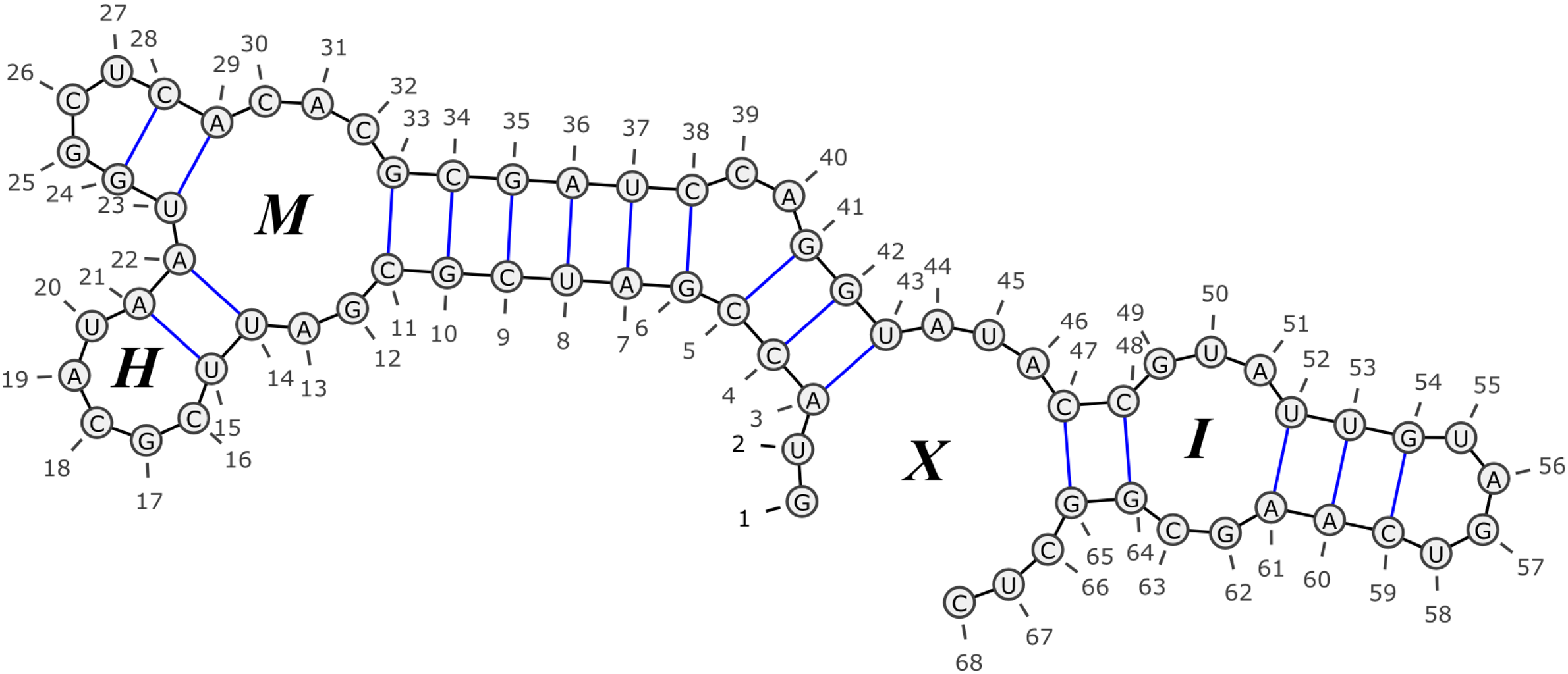
RNA secondary structure. Consecutive bases in the sequence are connected with (short) black edges, where base-pairs appear as blue (longer) edges. The labels within the loops stand for loop types, where H denotes a hairpin, I denotes an internal-loop, M denotes a multi-loop, and X denotes an external-loop. Drawing was made using the VARNA tool (Darty et al. 2009).

RNA structure prediction (henceforth RNA folding) is usually formulated as an optimization problem, where a score is defined for every possible folding of the given RNA sequence, and the predicted folding is one that maximizes this score. While finding a folding that maximizes the score under an arbitrary scoring function is intractable due to the magnitude of the search space, specific classes of scoring functions allow for an efficient solution using dynamic programming (Nussinov and Jacobson, 1980). Thus, in the standard scoring approach, the score assigned to a folding is composed as the sum of scores of local structural elements, where the set of local elements are chosen to allow efficient dynamic programming inference.1

Several scoring models were introduced over the past three decades, where these models mainly differ in the types of structural elements they examine (the feature-set), and the scores they assign to them. A simple example of such a model is the one of Nussinov and Jacobson (1980), which defines a single feature corresponding to a canonical Watson-Crick base-pair in the structure (i.e., base-pairs of the form G-C and A-U, and their respective reversed forms). The score of each occurrence of the feature in the structure is 1, and thus the total score of a folding is simply the number of canonical base-pairs it contains. A more complex model, which is commonly referred to as the Turner99 model, was defined in Mathews et al. (1999b) and is widely used in RNA structure prediction systems (Hofacker et al., 2002; Zuker, 1989, 2003). This model distinguishes between several different types of structural elements corresponding to unpaired bases, base-pairs which participate in different types of loops, loop-length elements, etc. In addition, every structural element can be mapped to one of several features, depending on some sequential context (e.g., the type of nucleotides at base-pair endpoints and within their vicinity), or other values (e.g., the specific loop length, internal-loop asymmetry value).

The parameter values (i.e., scores of each local element) are traditionally obtained from wet-lab experiments (Mathews et al., 1999a), reflecting the thermodynamics free energy theory (Tinoco et al., 1971, 1973). However, the increasing availability of known RNA structures in current RNA databases (Griffiths-Jones et al., 2005) makes it possible to conduct an improved, fine-tuned parameter estimation based on machine-learning (ML) techniques, resulting in higher prediction accuracies. These methods examine large training sets, composed of RNA sequences and their known structures (Sakakibara et al., 1994; Eddy and Durbin, 1994; Dowell and Eddy, 2004; Do et al., 2006, 2007; Andronescu et al., 2007, 2010).

Do et al. (2006) proposed to set the parameters by fitting an SCFG-based conditional log-linear model to maximize the conditional log-likelihood of a set of known structures. The approach was extended in Do et al. (2007) to include automatic tuning of regularization hyperparameters. Andronescu et al. (2007, 2010) used the Turner99 model, and applied Constraint-Generation (CG) and Boltzman-likelihood (BL) methods for the parameters estimation. These methods start with a set of wet-lab parameter values, and refine them using a training set of RNA sequences and their known structures, and an additional data set containing triplets of sequences, structures, and their measured thermodynamic energies. The parameters derived by Andronescu et al. (2010) yield the best published results for RNA folding prediction to date, when tested on a large structural data set.

While the methods for parameter estimation are successfully shifting toward ML-based approaches, the model parameterizations have so far remained fairly constant. Originating from the practice of setting the parameter values using wet-lab measurements, most models to date have relatively few parameters, where each parameter corresponds to the score of one particular local configuration.

We propose a move to much richer parameterizations, which is made possible due to the availability of large training sets (Andronescu et al., 2008) combined with advances in machine-learning (Collins, 2002; Crammer et al., 2006), and supported in practice by recent accelerations to RNA folding algorithms (Wexler et al., 2007; Backofen et al., 2011). The scoring models we apply refine previous models by examining more types of structural elements, and a larger sequential context for these elements. Based on this, similar structural elements could get scored differently in different sequential contexts, and different structural elements may get similar scores in similar sequential contexts.

We base our models on the structural elements defined by the Turner99 model in order to facilitate efficient inference. However, in our models, the score assigned to each structural element is itself composed of the sum of scores of many fine-grained local features that take into account portions of larger structural and sequential context. While previous models usually assign a single score to each element (e.g., the base-pair between positions 5 and 41 in Fig. 1), our models score elements as a sum of scores of various features (e.g., the base-pair (5, 41) has the features of being a right-bulge closing base-pair, participating in a stem, having its left endpoint centering a CCG sequence, starting a CGA sequence, and various other contextual factors).

Our final model has about 70,000 free parameters, several orders of magnitude more than previous models. We show that we are still able to effectively set the parameter values based on several thousands of training examples. Our resulting models yield a significant improvement in the prediction accuracy over the previous best results reported by Andronescu et al. (2010), when trained and tested over the same data sets. Our ContextFold tool, as well as the various trained models, are freely available at www.cs.bgu.ac.il/∼negevcb/contextfold and allow for efficient training and inference. In addition to reproducing the results in this work, it also provides flexible means for further experimenting with different forms of richer parameterizations.

2. Preliminaries and Problem Definition

For an RNA sequence x, denote by Y_x the domain of all possible foldings of x. We represent foldings as sets of index-pairs of the form (i, j), i < j, where each pair corresponds to two positions in the sequence such that the bases in these positions are paired. We use the notation (x, y) for a sequence-folding pair, where x is an RNA sequence and y is the folding of x. A scoring model G is a function that assigns real-value scores to sequence-folding pairs (x, y). For a given scoring model G, the RNA folding prediction problem is defined as follows2: given an RNA sequence x, find a folding \documentclass{aastex}\usepackage{amsbsy}\usepackage{amsfonts}\usepackage{amssymb}\usepackage{bm}\usepackage{mathrsfs}\usepackage{pifont}\usepackage{stmaryrd}\usepackage{textcomp}\usepackage{portland, xspace}\usepackage{amsmath, amsxtra}\pagestyle{empty}\DeclareMathSizes{10}{9}{7}{6}\begin{document} $$\hat{y} \in Y_x$$ \end{document} s.t. \documentclass{aastex}\usepackage{amsbsy}\usepackage{amsfonts}\usepackage{amssymb}\usepackage{bm}\usepackage{mathrsfs}\usepackage{pifont}\usepackage{stmaryrd}\usepackage{textcomp}\usepackage{portland, xspace}\usepackage{amsmath, amsxtra}\pagestyle{empty}\DeclareMathSizes{10}{9}{7}{6}\begin{document} $$G (x , \hat{y})$$ \end{document} is maximal. Such a folding \documentclass{aastex}\usepackage{amsbsy}\usepackage{amsfonts}\usepackage{amssymb}\usepackage{bm}\usepackage{mathrsfs}\usepackage{pifont}\usepackage{stmaryrd}\usepackage{textcomp}\usepackage{portland, xspace}\usepackage{amsmath, amsxtra}\pagestyle{empty}\DeclareMathSizes{10}{9}{7}{6}\begin{document} $$\hat{y}$$ \end{document} will be called an optimal folding for x with respect to G. A folding prediction (or a decoding) algorithm f_G is an algorithm that solves the folding prediction problem, i.e., \documentclass{aastex}\usepackage{amsbsy}\usepackage{amsfonts}\usepackage{amssymb}\usepackage{bm}\usepackage{mathrsfs}\usepackage{pifont}\usepackage{stmaryrd}\usepackage{textcomp}\usepackage{portland, xspace}\usepackage{amsmath, amsxtra}\pagestyle{empty}\DeclareMathSizes{10}{9}{7}{6}\begin{document} \begin{align*}\hat{y} = f_G (x) = {\rm argmax}_{y \in Y_x} \{G (x , y) \} \tag{1}\end{align*} \end{document}

Denote by ρ a cost function measuring a distance between two foldings, satisfying ρ(y, y) = 0 for every y and ρ(y, y′) > 0 for every y ≠ y′. This function indicates the cost associated with predicting the structure y′ where the real structure is y. For RNA folding, this cost is usually defined in terms of sensitivity, PPV, and F-measure (see Section 5). Intuitively, a good scoring model G is one such that ρ(y, f_G(x)) is small for arbitrary RNA sequences x and their corresponding true foldings y.

In order to allow for efficient computation of f_G, the score G(x, y) is usually computed on the basis of various local features of the pair (x, y). These features correspond to some structural elements induced by y, possibly restricted to appear in some specific sequential context in x. An example of such a feature could be the presence of a stem where the first base-pair in the stem is C-G and it is followed by the base-pair A-U. We denote by Φ the set of different features which are considered by the model, where Φ defines a finite number N of such features. The notation Φ(x, y) denotes the feature representation of (x, y), i.e., the collection of occurrences of features from Φ in (x, y). We assume that every occurrence of a feature is assigned a real-value, which reflects the “strength” of the occurrence. For example, we may define a feature corresponding to the interval of unpaired bases within a hairpin, and define that the value of an occurrence of this feature is the log of the interval length. For binary features such as the stem-feature described above, occurrence values are taken to be 1.

In order to score a pair (x, y), we compute scores for feature occurrences in the pair, and sum up these scores. Each feature in Φ is associated with a corresponding score (or a weight), and the score of a specific occurrence of a feature in (x, y) is defined to be the value of the occurrence multiplied by the corresponding feature weight. Φ(x, y) can be represented as a vector of length N, in which the ith entry φ_i corresponds to the ith feature in Φ. Since the same feature may occur several times in (x, y) (e.g., two occurrences of a stem), the value φ_i is taken to be the sum of values of the corresponding feature occurrences. Formally, this defines a linear model: \documentclass{aastex}\usepackage{amsbsy}\usepackage{amsfonts}\usepackage{amssymb}\usepackage{bm}\usepackage{mathrsfs}\usepackage{pifont}\usepackage{stmaryrd}\usepackage{textcomp}\usepackage{portland, xspace}\usepackage{amsmath, amsxtra}\pagestyle{empty}\DeclareMathSizes{10}{9}{7}{6}\begin{document} \begin{align*}G (x , y) = \mathop\sum_{\phi_i \in \Phi (x , y)} \phi_i {\bf w}_i = \Phi (x , y) ^T \cdot {\bf w} \tag{2}\end{align*} \end{document}

where w is a weight vector in which w_i is the weight of the ith feature in Φ, and · is the dot-product operator. The vector w of N feature weights is called the model parameters, and Φ is thus referred to as the model parameterization. We use the notation G_Φ,w to indicate a scoring model G with the specific parameterization Φ and parameters w.

The predictive quality of a model of the form G_Φ,w depends both on the parameterization Φ, defining which features are examined, and on the specific weights in w which dictate how to score these features. Having fixed a model parameterization Φ, the model parameter values w can be set based on scientific intuitions and on biological measurements (as done in thermodynamic based models), or based on statistical estimation over observed (x, y) pairs using machine-learning techniques. Aiming to design better models of the form G_Φ,w, there is a need to balance between (a) choosing a rich and informative parameterization Φ so that with optimal weights w the prediction quality of the model will be as good as possible, (b) allowing for a tractable folding prediction algorithm \documentclass{aastex}\usepackage{amsbsy}\usepackage{amsfonts}\usepackage{amssymb}\usepackage{bm}\usepackage{mathrsfs}\usepackage{pifont}\usepackage{stmaryrd}\usepackage{textcomp}\usepackage{portland, xspace}\usepackage{amsmath, amsxtra}\pagestyle{empty}\DeclareMathSizes{10}{9}{7}{6}\begin{document} $$f_{G_{\Phi , {\bf w}}}$$ \end{document} , and (c) being able to estimate optimal (or at least “good”) weight parameters w.

3. Feature Representations

We argue that with suitable learning techniques, not being tied to features whose weights could be determined experimentally, and having a large enough set of examples (x, y) such that y is the true folding of x, one could define much richer feature representations than was previously explored, while still allowing efficient inference. These richer representations allow the models to condition on many more fragments of information when scoring the various foldings for a given sequence x, and consequently come up with better predictions. This section describes the types of features incorporated in our models.

All examples in this section refer to the folding depicted in Figure 1, and we assume that the reader is familiar with the standard RNA folding terminology. The considered features broadly resemble those used in the Turner99 model, with some additions and refinements described below, and allow for an efficient Zuker-like dynamic programming folding prediction algorithm (Zuker and Stiegler, 1981). Formal definitions of some of the terms we use, as well as the exact feature representations we apply in the various models, can be found in Section A of the Appendix.

We consider two kinds of features: binary features and real-valued features.

Binary features. Binary features are features for which occurrence values are always 1; thus, the scores of such occurrences are simply the corresponding feature weights. These features occur in a sequence-folding pair whenever some specific structural element is present in some specific sequential context. The set of structural elements contains base-pairs and unpaired bases, which appear in loops of specific types, for example a multi-loop closing a base-pair, or an unpaired base within a hairpin. A sequential context describes the identities of bases appearing in some given offsets with respect to the location of the structural element in the sequence, for example, the presence of bases of types C and G at the two endpoints (i, j) of a base-pair. A complete example of such a binary feature is hairpin_base_0=G_+1=C_−2=U, indicating the presence of an unpaired-base of type G inside a hairpin at a sequence position i, while positions i + 1 and i − 2 contain bases of types C and U respectively. This feature will be generated for the unpaired-bases at positions 17 and 25 in Figure 1.

In contrast to most previous models, where each structural element is considered with respect to a single sequential context (and producing exactly one scoring term), in our models the score of a structural element is itself a linear combination of different scores of various (possibly overlapping) pieces of information. For example, a model may contain the features hairpin_base_−1=C_−2=U and hairpin_base_0=G_+1=C_−1=C which will also be generated for the unpaired-base in position 17 (thus differentiating it from the unpaired base at position 25). Note that the appearance of a C-base at relative position −1 appears in both of these features, demonstrating overlapping information regarded by the two features. The decomposition of the sequential context into various overlapping fragments allows us to consider broader and more refined sequential contexts compared to previous models.

The structural information we allow is also more refined than in previous models: we consider properties of the elements, such as loop lengths (e.g., a base-pair which closes a hairpin of length 3 may be scored differently than a base-pair which closes a hairpin of length 4, even if the examined sequential contexts of the two base-pairs are identical), and examine the two orientations of each base-pair (e.g., the base-pair (11, 33) may be considered as a C-G closing base-pair of the multi-loop marked with an M, and it may also be considered as a G-C opening base-pair of the stem that consists of the base-pair (10, 34) in addition to this base-pair). We distinguish between unpaired bases at the “shorter” and “longer” sides of an internal-loop, and distinguish between unpaired bases in external intervals, depending on whether they are at the 5′-end, 3′-end, or neither (i.e., the intervals 1–2, 66–68, and 44–46, respectively). Notably, our refined structural classification allows for the generalization of the concept of “bulges”, where, for example, it is possible to define special internal-loop types such that the left length of the loop is exactly k (up to some predefined maximum value for k), and the right length is at least k, and to assign specific features for unpaired bases and base-pairs which participate in such loops.

Real-valued features. Another kind of structural information not covered by the binary unpaired base features and base-pair features is captured by a set of real-valued length features. These features are generated with respect to intervals of unpaired bases, such as the three types of external intervals (as mentioned above), intervals of unpaired bases within hairpins (e.g., the interval 16–20 in the example), and intervals of unpaired bases within internal-loops up to some predefined length bound3 (e.g., the interval 49–51). The value of an occurrence of a length feature can be any function of the corresponding interval length. In this work, we follow the argumentation of Mathews et al. (1999b) and set the values to be the log of the interval length. As mentioned above, the structural base-pairs and unpaired-bases information is conjoined with various pieces of contextual information. We currently do not consider contextual information for the real-valued length features.

Our features provide varied sources of structural and contextual information. We rely on a learning algorithm to come up with suitable weights for all these bits and pieces of information.

4. Learning Algorithm

The learning algorithm we use is inspired by the discriminative structured-prediction learning framework proposed by Collins (2002) for learning in natural language settings, coupled with a passive-aggressive online learning algorithm (Crammer et al., 2006). Algorithms in this class adapt well to large feature sets, do not require the features to be independent, cope well with irrelevant features, and were shown to perform well in numerous natural language settings (Chiang et al., 2009; McDonald et al., 2005; Watanabe et al., 2010). Here, we demonstrate they provide state-of-the-art results also for RNA folding. The learning algorithm is simple to understand and to implement, and has strong formal guarantees. In addition, it considers one training instance (sequence-folding pair) at a time, making it scale linearly in the number of training examples in terms of computation time, and have a memory requirement which depends on the longest training example.

Recall the goal of the learning algorithm: given a feature representation Φ, a folding algorithm \documentclass{aastex}\usepackage{amsbsy}\usepackage{amsfonts}\usepackage{amssymb}\usepackage{bm}\usepackage{mathrsfs}\usepackage{pifont}\usepackage{stmaryrd}\usepackage{textcomp}\usepackage{portland, xspace}\usepackage{amsmath, amsxtra}\pagestyle{empty}\DeclareMathSizes{10}{9}{7}{6}\begin{document} $$f_{G_{\Phi , {\bf w}}}$$ \end{document} , a cost function ρ and a set of training instances S_train, find a set of parameter values w such that the expected cost \documentclass{aastex}\usepackage{amsbsy}\usepackage{amsfonts}\usepackage{amssymb}\usepackage{bm}\usepackage{mathrsfs}\usepackage{pifont}\usepackage{stmaryrd}\usepackage{textcomp}\usepackage{portland, xspace}\usepackage{amsmath, amsxtra}\pagestyle{empty}\DeclareMathSizes{10}{9}{7}{6}\begin{document} $$\rho (y , f_{G_{\Phi , {\bf w}}} (x))$$ \end{document} over unseen sequences x and their true foldings y is minimal.

The algorithm works in rounds. Denote by w⁰ = 0 the initial values in the parameter vector maintained by the algorithm. At each iteration i the algorithm is presented with a pair \documentclass{aastex}\usepackage{amsbsy}\usepackage{amsfonts}\usepackage{amssymb}\usepackage{bm}\usepackage{mathrsfs}\usepackage{pifont}\usepackage{stmaryrd}\usepackage{textcomp}\usepackage{portland, xspace}\usepackage{amsmath, amsxtra}\pagestyle{empty}\DeclareMathSizes{10}{9}{7}{6}\begin{document} $$(x , y) \in S_{train}$$ \end{document} . It uses its current parameters wⁱ⁻¹ to obtain \documentclass{aastex}\usepackage{amsbsy}\usepackage{amsfonts}\usepackage{amssymb}\usepackage{bm}\usepackage{mathrsfs}\usepackage{pifont}\usepackage{stmaryrd}\usepackage{textcomp}\usepackage{portland, xspace}\usepackage{amsmath, amsxtra}\pagestyle{empty}\DeclareMathSizes{10}{9}{7}{6}\begin{document} $$\hat{y} = f_{G_{\Phi , {\bf w}^{i - 1}}} (x)$$ \end{document} , and updates the parameter vector according to: \documentclass{aastex}\usepackage{amsbsy}\usepackage{amsfonts}\usepackage{amssymb}\usepackage{bm}\usepackage{mathrsfs}\usepackage{pifont}\usepackage{stmaryrd}\usepackage{textcomp}\usepackage{portland, xspace}\usepackage{amsmath, amsxtra}\pagestyle{empty}\DeclareMathSizes{10}{9}{7}{6}\begin{document} \begin{align*} {\bf w}^{i} = \begin{cases} {\bf w}^{i - 1} , & \rho (y , \hat{y}) = 0 , \\ {\bf w}^{i - 1} + \tau_i \Phi (x , y) - \tau_i \Phi (x , \hat{y}) , & {\rm otherwise}, \end{cases} \tag{3} \end{align*} \end{document}

where: \documentclass{aastex}\usepackage{amsbsy}\usepackage{amsfonts}\usepackage{amssymb}\usepackage{bm}\usepackage{mathrsfs}\usepackage{pifont}\usepackage{stmaryrd}\usepackage{textcomp}\usepackage{portland, xspace}\usepackage{amsmath, amsxtra}\pagestyle{empty}\DeclareMathSizes{10}{9}{7}{6}\begin{document} \begin{align*}\tau_i = \min \left(1 , \frac {\Phi (x , \hat {y}) ^T \cdot {\bf w} ^ {i - 1} - \Phi (x , y) ^T \cdot {\bf w} ^ {i - 1} + \sqrt {\rho (y , \hat {y})}} {\mid \mid \Phi (x , \hat {y}) - \Phi (x , y) \mid \mid ^2} \right).\end{align*} \end{document}

This is the PA-I update for cost sensitive learning with structured outputs described in Crammer et al. (2006). Loosely, Equation 3 attempts to set wⁱ such that the correct structure y would score higher than the predicted structure \documentclass{aastex}\usepackage{amsbsy}\usepackage{amsfonts}\usepackage{amssymb}\usepackage{bm}\usepackage{mathrsfs}\usepackage{pifont}\usepackage{stmaryrd}\usepackage{textcomp}\usepackage{portland, xspace}\usepackage{amsmath, amsxtra}\pagestyle{empty}\DeclareMathSizes{10}{9}{7}{6}\begin{document} $$\hat{y}$$ \end{document} with a margin of at least the square-root of the difference between the structures, while trying to minimize the change from wⁱ⁻¹ to wⁱ. This is achieved by decreasing the weights of features appearing only in the predicted structure, and increasing the weights of features appearing only in the correct structure. Even though one example is considered at a time, the procedure is guaranteed to converge to a good set of parameter values. For the theoretical convergence bounds and proofs, see Crammer et al. (2006). In practice, due to the finite size of the training data, the algorithm is run for several passes over the training set.4

In order to avoid over-fitting of the training data, the final w is taken to be the average over all wⁱ seen in training. That is, \documentclass{aastex}\usepackage{amsbsy}\usepackage{amsfonts}\usepackage{amssymb}\usepackage{bm}\usepackage{mathrsfs}\usepackage{pifont}\usepackage{stmaryrd}\usepackage{textcomp}\usepackage{portland, xspace}\usepackage{amsmath, amsxtra}\pagestyle{empty}\DeclareMathSizes{10}{9}{7}{6}\begin{document} $${\bf w} ^ {final} = \frac {1} {K} \sum \nolimits_ {i = 1} ^ {K} {\bf w} ^i$$ \end{document} , where K is the number of processed instances. This widely used practice introduced in Freund and Schapire (1999) provides a regularization effect and improves the prediction results on unseen data.

5. Experiments

In order to test the effect of richer parameterizations on RNA prediction quality, we have conducted five learning experiments with increasingly richer model parameterizations, ranging from 226 active features for the simplest model to about 70,000 features for the most complex one.

5.1. Experiment settings

Feature representations. As described in Section 3, our features combine structural and contextual information. We begin with a baseline model (Baseline), which includes a trivial amount of contextual information (the identities of the two bases in a base-pair) and a set of basic structural elements such as hairpin unpaired base, internal-loop unpaired base, stem closing base-pair, multi-loop closing base-pair, and hairpin length. This baseline model has a potential of inducing up to 1,919 different features, but in practice about 220 features are assigned a non-zero weight after the training process, a number that is comparable to the number of parameters used in previously published models.

We then enrich this basic model with varying amounts of structural (St) and contextual (Co) information. St^med adds distinction between various kinds of short loops, considers the two orientations of each base-pair, and considers unpaired bases in external intervals, and St^high adds further length-based loop type refinements. Similarly, Co^med considers also the identities of unpaired bases and the base types of the adjacent pair (i + 1, j − 1) for each base-pair (i, j), while Co^high considers also the neighbors of unpaired bases and more configurations of neighbors surrounding a base-pair.

The models St^medCo^med, St^highCo^med, St^medCo^high and St^highCo^high can potentially induce about 14k, 30k, 86k, and 205k parameters, respectively, but in practice much fewer parameters are assigned non-zero values after training, resulting in effective parameter counts of 4k, 7k, 38k, and 70k. The exact definition of the different structural elements and sequential contexts considered in each model are provided in Section A of the Appendix.

Evaluation measures. We follow the common practice and assess the quality of our predictions based on the sensitivity, positive predictive value (PPV), and F₁-measure metrics, defined as \documentclass{aastex}\usepackage{amsbsy}\usepackage{amsfonts}\usepackage{amssymb}\usepackage{bm}\usepackage{mathrsfs}\usepackage{pifont}\usepackage{stmaryrd}\usepackage{textcomp}\usepackage{portland, xspace}\usepackage{amsmath, amsxtra}\pagestyle{empty}\DeclareMathSizes{10}{9}{7}{6}\begin{document} $$\frac {\mid y \cap \hat {y} \mid} {\mid y \mid}$$ \end{document} , \documentclass{aastex}\usepackage{amsbsy}\usepackage{amsfonts}\usepackage{amssymb}\usepackage{bm}\usepackage{mathrsfs}\usepackage{pifont}\usepackage{stmaryrd}\usepackage{textcomp}\usepackage{portland, xspace}\usepackage{amsmath, amsxtra}\pagestyle{empty}\DeclareMathSizes{10}{9}{7}{6}\begin{document} $$\frac {\mid y \cap \hat {y} \mid} {\mid \hat {y} \mid}$$ \end{document} , and \documentclass{aastex}\usepackage{amsbsy}\usepackage{amsfonts}\usepackage{amssymb}\usepackage{bm}\usepackage{mathrsfs}\usepackage{pifont}\usepackage{stmaryrd}\usepackage{textcomp}\usepackage{portland, xspace}\usepackage{amsmath, amsxtra}\pagestyle{empty}\DeclareMathSizes{10}{9}{7}{6}\begin{document} $$\frac {2 \mid y \cap \hat {y} \mid} {\mid y \mid + \mid \hat {y} \mid}$$ \end{document} , respectively, for a known structure y and a predicted structure \documentclass{aastex}\usepackage{amsbsy}\usepackage{amsfonts}\usepackage{amssymb}\usepackage{bm}\usepackage{mathrsfs}\usepackage{pifont}\usepackage{stmaryrd}\usepackage{textcomp}\usepackage{portland, xspace}\usepackage{amsmath, amsxtra}\pagestyle{empty}\DeclareMathSizes{10}{9}{7}{6}\begin{document} $$\hat{y}$$ \end{document} , where |y| is the number of base-pairs in a structure y, and \documentclass{aastex}\usepackage{amsbsy}\usepackage{amsfonts}\usepackage{amssymb}\usepackage{bm}\usepackage{mathrsfs}\usepackage{pifont}\usepackage{stmaryrd}\usepackage{textcomp}\usepackage{portland, xspace}\usepackage{amsmath, amsxtra}\pagestyle{empty}\DeclareMathSizes{10}{9}{7}{6}\begin{document} $$\mid y \cap \hat{y} \mid$$ \end{document} is the number of base-pairs appearing in both structures y and \documentclass{aastex}\usepackage{amsbsy}\usepackage{amsfonts}\usepackage{amssymb}\usepackage{bm}\usepackage{mathrsfs}\usepackage{pifont}\usepackage{stmaryrd}\usepackage{textcomp}\usepackage{portland, xspace}\usepackage{amsmath, amsxtra}\pagestyle{empty}\DeclareMathSizes{10}{9}{7}{6}\begin{document} $$\hat{y}$$ \end{document} . Sensitivity is the proportion of correctly predicted base-pairs among all true base-pairs, PPV is the proportion of correctly predicted base-pairs among all predicted base-pairs, and F₁ is a value which balances sensitivity and PPV. All of the measures range in value from 0 to 1, where a value of 1 indicates that the true and predicted structure are identical, and a value of 0 means that none of the true base-pairs in y are predicted in \documentclass{aastex}\usepackage{amsbsy}\usepackage{amsfonts}\usepackage{amssymb}\usepackage{bm}\usepackage{mathrsfs}\usepackage{pifont}\usepackage{stmaryrd}\usepackage{textcomp}\usepackage{portland, xspace}\usepackage{amsmath, amsxtra}\pagestyle{empty}\DeclareMathSizes{10}{9}{7}{6}\begin{document} $$\hat{y}$$ \end{document} . As in previous works, the reported scores are averaged over the scores of individual predicted structures in the test set.

Folding prediction algorithm. We implemented a new folding prediction algorithm, which supports the extended feature representations in our models. This implementation allows for a flexible model design, under which additional models, similarly structured to those presented here, may be defined. In addition, this is the first publicly available implementation to utilize the sparsification techniques, recently reported in Backofen et al. (2011) for accelerating the running time, over realistic models (weaker sparsification techniques were presented in Wexler et al. [2007] and applied by Ziv-Ukelson et al. [2008]; Salari et al. [2010, and Möhl et al. [2010]). See Section B of the Appendix for sparsification statistics. The code is publicly available on our website.

Learning setup. The learning algorithm iterates over the training data, halting as soon as the performance over this data does not significantly improve for three iterations in a row. The order of the training examples is shuffled prior to each iteration. As the learning algorithm allows for optimization against arbitrary cost functions, we chose the one which is directly related to our evaluation measure, namely \documentclass{aastex}\usepackage{amsbsy}\usepackage{amsfonts}\usepackage{amssymb}\usepackage{bm}\usepackage{mathrsfs}\usepackage{pifont}\usepackage{stmaryrd}\usepackage{textcomp}\usepackage{portland, xspace}\usepackage{amsmath, amsxtra}\pagestyle{empty}\DeclareMathSizes{10}{9}{7}{6}\begin{document} $$\rho (y , \hat{y}) = 1 - F_1 (y , \hat{y})$$ \end{document} . The final weight vector is taken to be the average of all computed vectors up to the last iteration. Parameters with absolute value smaller than 0.01 of the maximal absolute parameter value are ignored.

Datasets. Our experiments are based on a large set of known RNA secondary structures. Specifically, we use the exact same data as used in the comprehensive experiments of Andronescu et al. (2010), including the same preprocessing steps, train/test/dev splits and naming conventions. We list some key properties of the data below, and refer the reader to Andronescu et al. (2010) for the remaining details. The complete data (S-Full) is based on the RNA STRAND dataset (Andronescu et al. 2008), and contains known RNA secondary structures for a diverse set of RNA families across various organisms. This data has gone through several preprocessing steps, including the removal of pseudoknots and non-canonical base-pairs. Overall, there are 3245 distinct structures, ranging in length from 10 to 700 nucleotides, with the average length being 269.6. The data is randomly split into S-Full-Train (80%) and S-Full-Test (20%), yielding the train and test sets respectively. S-Full-Train is further split into S-Full-Alg-Train (80% of S-Full-Train) and S-Full-Alg-Val (the remaining 20%) (this partition of the data is the same as in Andronescu [2008]). We use S-Full-Alg-Train and S-Full-Alg-Val (the dev set) during the development and for most of the experiments, and reserve S-Full-Train and S-Full-Test for the final evaluation which is presented in Table 3.

5.2. Results

Convergence. Figure 2 shows the F₁ scores of the various models on the S-Full-Alg-Train training set as a function of the number of iterations. All models converge after less than 20 iterations, where models with more features take more iterations to converge. Training is very fast: training the St^medCo^med model (about 4k effective features) takes about 2–3 minutes per iteration and less than half an hour in all on a single core of one Phenom II CPU, while training the St^highCo^high model (about 70k effective features) requires about 13–14 minutes per iteration and about 3–4 hours in all (in contrast, the CG models described in Andronescu et al. [2007, 2010] are reported to take 1.1–3.1 days of cpu-time to train, and the BL models take up to 200 days to train). None of the models achieve perfect scores on the training set, indicating that even our richest feature representation does not capture all the relevant information governing the folding process. However, the training set results clearly support our hypothesis: having more features increases the ability of the model to explain the observed data.

FIG. 2.

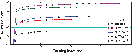
Performance on S-Full-Alg-Train as a function of the number of training iterations.

Validation accuracy. Train-set performance is not a guarantee of good predictive power. Therefore, the output models of the training procedure were tested on the independent set S-Full-Alg-Val. Table 1 shows the accuracies of the various models over this set. The results are expectedly lower than those over the training set, but the overall trends remain: adding more features significantly improves the performance. The contribution of the contextual feature (about 12–13 absolute F₁ points moving from St^medCo^med to St^medCo^high and from St^highCo^med to St^highCo^high) is larger than that of the structural features (about three absolute F₁ points moving from St^medCo^med to St^highCo^med and from St^medCo^high to St^highCo^high), but the contributions are mostly orthogonal – using richest structural and contextual information (St^highCo^high) further increases the results to an F₁ score of 83.2, an absolute F₁ improvement of 27.4 points over the baseline model.

Table 1.

Performance of the Different Models on the Development Set

Model	# Params	Sens (%)	PPV (%)	F ₁ (%)
Baseline	226	56.9	55.3	55.8
St^medCo^med	4,054	69.1	66.3	67.4
St^highCo^med	7,075	72.3	70.3	71.0
St^medCo^high	37,846	81.4	80.0	80.5
St^highCo^high	68,606	83.8	83.0	83.2

All models were trained on the training set S-Full-Alg-Train. The # Params column indicates the number of features to which a non-zero weight was assign (after filtering out parameters whose absolute value is lower than 0.01 of the maximum absolute parameter value). Columns Sens, PPV, and F₁ give the sesitivity, PPV, and F₁ values, respectively (in percentage), measured on the S-Full-Alg-Val dataset.

Stability. We performed a fivefold cross-validation experiment to verify that the results do not depend on a particular train-test split. We randomly shuffled S-Full-Train and performed five test-train splits, each of them reserving a different 20% of the data for testing and training on the rest. The results on the folds are similar to those on the development set with a maximum deviation of about ± 1 F₁ points from the numbers in Table 1.

Effect of training-set size. We investigated the effect of the training-set size on the predictive quality of the model by artificially training our models on small subsets of S-Full-Alg-Train. Figure 3 presents the learning curves for these experiments.

FIG. 3.

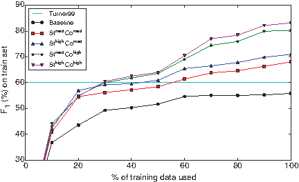
Effect of training set size on validation-set accuracies.

Performance clearly increases as more examples are included in the training. The curve for the Baseline feature-set flattens out at about 60% of the training data, but the curves of the feature-rich models indicate that further improvement is possible with more training data. Thirty percent of the training data is sufficient for St^medCo^high and St^highCo^high to achieve the performance of the Turner99 model, and all but the Baseline feature set surpass the Turner99 performance with 60% of the training data.

Results by RNA family. The dataset we use contains a diverse set of RNA structures, coming from many RNA families. The dataset is then split randomly into training and testing parts, where RNA types distribute similarly in each of these parts. The algorithm then learns both general properties of all RNA families, as well as family specific parameter values. The RNA family information is not available to either the training or prediction algorithms, which are based only on the sequence information. Still, higher performance rates are expected for RNA families which were available during training.

Table 2 shows the accuracies of the models on the different RNA families appearing in the development set. Interestingly, while the richest St^highCo^high model achieves the highest scores when averaged over the entire dev set, some families (mostly those of shorter RNA sequences) are better predicted by the simpler St^highCo^med and St^medCo^high models. Our machine-learned models significantly outperform the energy-based Turner99 model on all RNA families, where the effect is especially pronounced on the 5S Ribosomal RNA, Transfer RNA and Transfer Messenger RNA families, for which even the relatively simple St^medCo^med model already outperform the energy-based model by a very wide margin.

Table 2.

Performance of the Different Models on the Development Set, Grouped by RNA Family

Familiy (# instances)	St^medCo^med	St^highCo^med	St^medCo^high	St^highCo^high	Turner99	CG ^*	BL-FR ^*
Hammerhead Ribozyme(12)	57.9	58.3	69.8	78.8	43.9	45.8	40.7
Group I Intron(11)	55.2	58.7	73.5	70.5	60.4	60.7	30.5
Cis-regulatory element(11)	45.9	46.1	81.8	85.2	61.1	61.2	74.0
Transfer Messenger RNA(70)	55.2	57.6	69.7	70.8	37.5	49.7	57.0
5S Ribosomal RNA(27)	89.2	90.9	94.1	93.9	68.9	79.9	86.4
Unknown(48)	93.9	94.1	95.7	94.8	91.14	92.3	92.5
Ribonuclease P RNA(72)	62.0	70.3	84.7	87.7	58.6	61.2	61.6
16S Ribosomal RNA(112)	57.9	65.4	81.0	86.3	55.2	62.3	66.6
Signal Recognition Particle RNA(62)	61.8	62.7	72.6	76.2	66.6	64.5	68.4
Transfer RNA(80)	91.8	94.2	92.2	92.8	60.7	79.1	81.5
23S Ribosomal RNA(28)	53.6	54.0	61.2	68.6	58.5	60.5	61.7
Other RNA(11)	65.9	66.4	71.8	73.5	61.1	62.0	74.1

Only families with more than 10 examples in the development test set are included. The highest score for each family appears in bold. The CG^* and BL-FR^* columns were obtained by running the software of Andronescu et al. (2010) with the corresponding models (note that the parameters for these models were obtained by training on the entire S-Full-Train set, while the parameters for our models were obtained by training on the partial set S-Full-Alg-Train).

Performance on novel RNA families. An interesting question is how our predictor will behave on completely novel RNA families, which were not available during training. In order to quantify this, we conducted another set of experiments. For five of the bigger families, the St^highCo^high model was trained after excluding all family members, and then performance was measured over the excluded family members. The procedure was then repeated, when 5, 10, and 20 (random) family members were added to the training set (performance is measured only on those members excluded from the training set). Figure 4 presents the results of this experiment.

FIG. 4.

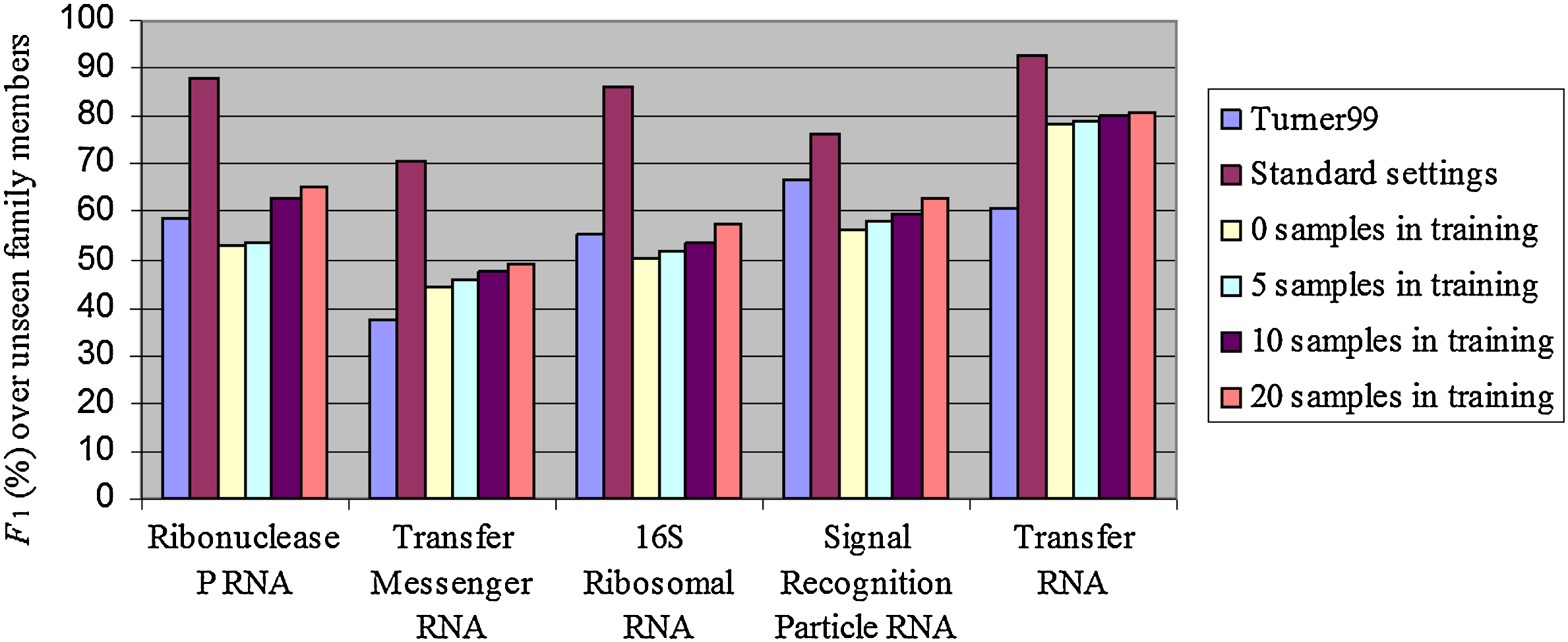
Performance over RNA families which were excluded from the training data. The Turner99 and Standard settings bars give the corresponding family performances in Table 2 of the Turner99 and the St^HighCo^High (trained over S-Full-Alg-Train) models, measured over family members in S-Full-Alg-Val, and are added for reference.

The prediction accuracies over completely unseen RNA types are comparable with those of the Turner99 model, indicating that our algorithm indeed learned general properties of RNA secondary structure. However, results are still considerably lower than those where there is a sufficient coverage of the family in the training set. This may indicate that different RNA families exhibit different features or are folded according to different rules, and that this kind of information may not be transferable across RNA families, at least not when considering the surface sequence alone. However, once the algorithm has seen enough examples of a family in order to effectively learn the parameters governing its folding process, it does a good job at identifying the correct family and folding it accordingly.

Final results. Finally, we train our models on the entire training set and evaluate them on the test set. Results on the test set are somewhat higher than on the dev set. In order to put the numbers in context, Table 3 presents the final scores together with the performance of other recent structural prediction systems over the same datasets. The scores of the other systems are taken from Andronescu et al. (2010) and to the best of our knowledge represent the current state-of-the-art for RNA secondary structure prediction.

Table 3.

Final Results on the Test Set

Model	Reference	# Params	Sens (%)	PPV (%)	F₁ (%)
Turner99	Mathews et al. (1999b)	363	62.7	57.6	59.8
‡† BL-FR^*	Andronescu et al. (2010)	7,726	71.4	68.1	69.5
‡† BL^*	Andronescu et al. (2010)	363	69.7	66.3	67.7
‡† LAM-CG (CG^*)	Andronescu et al. (2010)	363	68.7	65.5	66.8
‡† NOM-CG	Andronescu et al. (2010)	363	68.2	64. 0	65.8
⋆ CONTRAFold 2.0	Do et al. (2006, 2007)	714	65.1	66.9	65.5
‡ St^medCo^med		4040	71.2	67.7	69.2
‡ St^highCo^med		7150	74.6	71.5	72.8
‡ St^medCo^high		37866	81.5	79.7	80.4
‡ St^highCo^high		69,603	85.0	83.7	84.1

Results of previous models are as reported in Andronescu et al. (2010). Models marked with ‡ are trained on S-Full-Train. The model marked with ⋆ is trained on S-Processed, a larger dataset than S-Full-Train (defined in Andronescu et al. (2007)) which contains some sequences from S-Full-Test. In the models marked with †, training is initialized with the Turner99 parameters, and uses additional thermodynamics information regarding the free energies of 1291 known structures.

The Baseline model with only 226 parameters achieves scores comparable to those of the Turner-99 model, despite being very simple, learned completely from data and not containing any physics-based measurements. Our simplest feature-rich model, St^medCo^med, having 4,040 parameters, is already slightly better than all but one of the previously best reported results, where the only better model (BL-FR) being itself a feature-rich model obtained by considering many feature-interactions between the various Truner99 parameters. Adding more features further improves the results, and our richest model, St^highCo^high, achieves a score of 84.1 F₁ on the test set – an absolute improvement of 14.4 F₁-points over the previously published best results for this data, amounting to an error reduction of about 50%. Note that the presented numbers reflect the prediction accurcy of the algorithms with respect to a specific dataset. While it is likely that similar accurcy levels would be obtained for new RNAs that belong to RNA families which are covered by the testing data, little can be said about accurcy levels for other RNA families.

6. Discussion

We showed that a move towards richer parameterizations is beneficial to ML-based RNA structure prediction. Indeed, our best model yields an error reduction of 50% from the previously best published results, under the same experimental conditions. Our learning curves relative to the amount of training data indicate that adding more data is likely to increase these already good results. While prediction quality is evidentially higher when predicting foldings of RNA sequences from families that were accessible to the training procedure, it is not inferior with respect to the prediction quality of energy-based models over sequences from unseen families. It is likely that better parameterizations are possible, and the search for a better richly-parameterized model is a fertile ground for exploration.

Our method has some limitations with respect to the physics-based models. In particular, our models scores do not represent free energies. However, there is no reason to use the same model for both structure prediction and free-energy estimation, which can be considered as two independent tasks. Instead, one model can be used for structure-prediction, and the free-energy of the predicted structure can be estimated using a different model which is tailored specifically to the energy-prediction task. Decoupling of structure-prediction and energy estimation is potentially beneficial for both tasks, as there is evidence that the final RNA structures do not neccessarily have the lowest energy among all the possible structures.

Another shortcoming of our current approach is that while it considers a single, margin-based, error-driven parameter estimation method and is optimized to predict one single best structure, it cannot compute the partition function, base-pair binding probabilities and centroid structures derived from them. Probabilistic, marginals-based (i.e., partition function based) training and decoding is an appealing alternative.

Finally, as the learned parameter weights are currently not interpretable, we would like to explore methods of analyzing and trying to make biological sense of them.

7. Appendix

A. Model descriptions

We specify here the features that are used by our models. Each feature description is composed of two parts: a description of a structural element, and a (possibly empty) description of a sequential context. All models discussed in the article are obtained by combining a set of structural elements St with a set of sequential contexts Co, and producing all corresponding features (i.e. producing a feature for each structural element in St and a corresponding sequential context from Co). In Section A.1, we define the different loop types, which are used for categorizing structural elements. In Section A.2, we give the three sets of structural elements St^base, St^med, and St^high, and in Section A.3, we give the three sets of sequential contexts Co^base, Co^med, and Co^high, which are used in our models.

The experiments in the article were conducted with respect to five scoring models: Baseline = St^baseCo^base, St^medCo^med, St^highCo^med, St^medCo^high, and St^highCo^high. Unpaired base features were obtained by taking each unpaired base structural element in the St set, and combining it with each single position sequential context defined in the Co set. Base-pair features were obtained by taking each base-pair structural element in the St set, and combining it with each double position sequential context defined in the Co set. Length features were obtained only from the St set, as described in Section A.2.

All examples in the text refer to the sequence-folding (x, y) depicted in Figure 1.

A.1 Loop definitions

Let y be a folding (of some RNA sequence x), and let (i, j) be a base-pair in y. Say that a base-pair \documentclass{aastex}\usepackage{amsbsy}\usepackage{amsfonts}\usepackage{amssymb}\usepackage{bm}\usepackage{mathrsfs}\usepackage{pifont}\usepackage{stmaryrd}\usepackage{textcomp}\usepackage{portland, xspace}\usepackage{amsmath, amsxtra}\pagestyle{empty}\DeclareMathSizes{10}{9}{7}{6}\begin{document} $$(p , q) \in y$$ \end{document} is covered by (i, j) if i < p < q < j. Similarly, for an unpaired base r in y, say that r is covered by (i, j) if i < r < j. Say that a base-pair (p, q) (an unpaired base r, resp.) is covered directly by (i, j) if it is covered by (i, j), and there is no other base-pair \documentclass{aastex}\usepackage{amsbsy}\usepackage{amsfonts}\usepackage{amssymb}\usepackage{bm}\usepackage{mathrsfs}\usepackage{pifont}\usepackage{stmaryrd}\usepackage{textcomp}\usepackage{portland, xspace}\usepackage{amsmath, amsxtra}\pagestyle{empty}\DeclareMathSizes{10}{9}{7}{6}\begin{document} $$(k , l) \in y$$ \end{document} covered by (i, j) such that (p, q) (r, resp.) is covered by (k, l). For example, the base-pair (11, 33) covers the base-pairs (23, 29) and (24, 28) and the unpaired bases 26 and 31, where (23, 29) and 31 are covered directly by (11, 33).

A loop is an entity which is composed from the following structural elements:

• Exactly one closing base-pair (i, j).

• A set of zero or more base-pairs which are covered directly by (i, j). Such base-pairs are called opening base-pairs of the loop.

• A set of zero or more unpaired bases which are covered directly by (i, j).

Loops are traditionally classified into three groups: hairpins (HP) are loops which do not have any opening base-pairs (as the loop closed by (15, 21)), internal-loops (IL) are loops which have a single opening base-pair (as the loop closed by (48, 64) and opened by (52, 61)), and multi-loops (ML) are loops which have more than one opening base-pair (as the loop closed by (11, 33), and opened by (14, 22) and by (23, 29)). Another group of “artificial” loops, which are called external-loops (XL), correspond to sets of elements which are not covered by any base-pair. External-loops may be thought of as loops which are closed by an artificial base-pair between positions 0 and |x| + 1 in the sequence, and may include zero or more opening base-pairs and zero or more unpaired bases (note that each folding of x defines exactly one external-loop, as the one marked with an X in the example; The latter external loop contains the opening base-pairs (3, 43) and (47, 65), and the unpaired base intervals 1–2, 44–46, 66–68).

In order to increase structural element granularity, we refine the hairpin and internal-loop categorization according to their lengths. The length of a hairpin closed by the base-pair (i, j) is defined to be j − i − 1 (i.e., the number of unpaired bases within the loop). An l-HP is the refined classification of all hairpins whose length is l. For example, the hairpin which is closed by the base-pair (15, 21) is a 5-HP. For each set of structural elements St which is defined in the next section, a parameter K was fixed, such that hairpins shorter than K were categorized according to their specific lengths, and hairpins of lengths K or above where categorized as “LONG-HP.”

For an internal loop which is closed by the base-pair (i, j) and is opened by the base-pair (p, q), the left and right lengths of the loop are the values p − i − 1 and j − q − 1, respectively. That is, the left length is the number of unpaired bases between i and p in the loop, and the right length is the number of unpaired bases between q and j. As for hairpins, internal loops are classified according to these lengths, where an “l-r-IL” is a classification of all internal-loops for which the left length is l and the right length is r. For example, the internal-loop closed by (48, 64) in the example (and opened by (52, 61)) is a 3-2-IL. Other traditional loop types such as stems (or stackings) and bulges can be viewed as special cases of internal-loops: a left bulge is an l-0-IL for some l > 0, a right bulge is a 0-r-IL for some r > 0, and a stem is a 0-0-IL. For each set of structural elements St, a parameter I and a series \documentclass{aastex}\usepackage{amsbsy}\usepackage{amsfonts}\usepackage{amssymb}\usepackage{bm}\usepackage{mathrsfs}\usepackage{pifont}\usepackage{stmaryrd}\usepackage{textcomp}\usepackage{portland, xspace}\usepackage{amsmath, amsxtra}\pagestyle{empty}\DeclareMathSizes{10}{9}{7}{6}\begin{document} $$I_0 , I_1 , \ldots , I_{I - 1}$$ \end{document} were fixed. An internal loop for which the length d of the shorter side is smaller than I and the length g of the longer side is shorter than I_d, is classified as d-g-IL or g-d-IL (depending on whether the shorter side is left or right, respectively). When the length of the longer side is at least I_d, the loop is classified as d-LONG-IL or LONG-d-IL, and if the length of the shorter side is at least I, it is a LONG-LONG-IL loop.

A.2. Structural elements

Structural elements of a sequence-folding pair (x, y) are inferred solely from the folding y (and the length of x), and do not consider the specific nucleotide composition of x. Each such element which is considered by our models either corresponds to a single base-pair, a single unpaired base, or an interval of unpaired bases. The elements are further categorized according to the loop in which they participate. Recall that y is represented as a set of index-pairs of the form (i, j), 1 ≤ i < j ≤ |x|, where a pair (i, j) in y indicates that the bases at positions i and j of the sequence x are paired in the folding. We say that a base r in x is unpaired in y, to indicate that there is no base-pair \documentclass{aastex}\usepackage{amsbsy}\usepackage{amsfonts}\usepackage{amssymb}\usepackage{bm}\usepackage{mathrsfs}\usepackage{pifont}\usepackage{stmaryrd}\usepackage{textcomp}\usepackage{portland, xspace}\usepackage{amsmath, amsxtra}\pagestyle{empty}\DeclareMathSizes{10}{9}{7}{6}\begin{document} $$(i , j) \in y$$ \end{document} such that r = i or r = j.

Base-pair elements are classified according to the loop type in which they participate, and whether they open or close this loop. The list of base-pair structural elements is summarized in Table 4.

Table 4.

Base-Pair Structural Element Types

Loop description	Closing base-pair type	Opening base-pair type
Hairpin closing base-pairs	3-HP-CLOSE	There are no hairpin opening base-pairs
	4-HP-CLOSE
	\documentclass{aastex}\usepackage{amsbsy}\usepackage{amsfonts}\usepackage{amssymb}\usepackage{bm}\usepackage{mathrsfs}\usepackage{pifont}\usepackage{stmaryrd}\usepackage{textcomp}\usepackage{portland, xspace}\usepackage{amsmath, amsxtra}\pagestyle{empty}\DeclareMathSizes{10}{9}{7}{6}\begin{document} $$\vdots$$ \end{document}
	(K − 1)-HP-CLOSE
	LONG-HP-CLOSE
Internal-loop terminating base-pairs, where the shorter loop length is 0 (i.e. “bulges”)	0-0-IL-CLOSE	0-0-IL-OPEN
	0-1-IL-CLOSE	0-1-IL-OPEN
	1-0-IL-CLOSE	1-0-IL-OPEN
	0-2-IL-CLOSE	0-2-IL-OPEN
	2-0-IL-CLOSE	2-0-IL-OPEN
	\documentclass{aastex}\usepackage{amsbsy}\usepackage{amsfonts}\usepackage{amssymb}\usepackage{bm}\usepackage{mathrsfs}\usepackage{pifont}\usepackage{stmaryrd}\usepackage{textcomp}\usepackage{portland, xspace}\usepackage{amsmath, amsxtra}\pagestyle{empty}\DeclareMathSizes{10}{9}{7}{6}\begin{document} $$\vdots$$ \end{document}	\documentclass{aastex}\usepackage{amsbsy}\usepackage{amsfonts}\usepackage{amssymb}\usepackage{bm}\usepackage{mathrsfs}\usepackage{pifont}\usepackage{stmaryrd}\usepackage{textcomp}\usepackage{portland, xspace}\usepackage{amsmath, amsxtra}\pagestyle{empty}\DeclareMathSizes{10}{9}{7}{6}\begin{document} $$\vdots$$ \end{document}
	0-(I₀ − 1)-IL-CLOSE	0-(I₀ − 1)-IL-OPEN
	(I₀ − 1)-0-IL-CLOSE	(I₀ − 1)-0-IL-OPEN
	0-LONG-IL-CLOSE	0-LONG-IL-OPEN
	LONG-0-IL-CLOSE	LONG-0-IL-OPEN
Internal-loop terminating base-pairs, where the shorter loop length is 1	1-1-IL-CLOSE	1-1-IL-OPEN
	1-2-IL-CLOSE	1-2-IL-OPEN
	2-1-IL-CLOSE	2-1-IL-OPEN
	\documentclass{aastex}\usepackage{amsbsy}\usepackage{amsfonts}\usepackage{amssymb}\usepackage{bm}\usepackage{mathrsfs}\usepackage{pifont}\usepackage{stmaryrd}\usepackage{textcomp}\usepackage{portland, xspace}\usepackage{amsmath, amsxtra}\pagestyle{empty}\DeclareMathSizes{10}{9}{7}{6}\begin{document} $$\vdots$$ \end{document}	\documentclass{aastex}\usepackage{amsbsy}\usepackage{amsfonts}\usepackage{amssymb}\usepackage{bm}\usepackage{mathrsfs}\usepackage{pifont}\usepackage{stmaryrd}\usepackage{textcomp}\usepackage{portland, xspace}\usepackage{amsmath, amsxtra}\pagestyle{empty}\DeclareMathSizes{10}{9}{7}{6}\begin{document} $$\vdots$$ \end{document}
	1-(I₁ − 1)-IL-CLOSE	1-(I₁ − 1)-IL-OPEN
	(I₁ − 1)-1-IL-CLOSE	(I₁ − 1)-1-IL-OPEN
	1-LONG-IL-CLOSE	1-LONG-IL-OPEN
	LONG-1-IL-CLOSE	LONG-1-IL-OPEN
Internal-loop terminating base-pairs, where the shorter loop length is I − 1	(I − 1)-(I − 1)-IL-CLOSE	(I − 1)-(I − 1)-IL-OPEN
	\documentclass{aastex}\usepackage{amsbsy}\usepackage{amsfonts}\usepackage{amssymb}\usepackage{bm}\usepackage{mathrsfs}\usepackage{pifont}\usepackage{stmaryrd}\usepackage{textcomp}\usepackage{portland, xspace}\usepackage{amsmath, amsxtra}\pagestyle{empty}\DeclareMathSizes{10}{9}{7}{6}\begin{document} $$\vdots$$ \end{document}	\documentclass{aastex}\usepackage{amsbsy}\usepackage{amsfonts}\usepackage{amssymb}\usepackage{bm}\usepackage{mathrsfs}\usepackage{pifont}\usepackage{stmaryrd}\usepackage{textcomp}\usepackage{portland, xspace}\usepackage{amsmath, amsxtra}\pagestyle{empty}\DeclareMathSizes{10}{9}{7}{6}\begin{document} $$\vdots$$ \end{document}
	(I − 1)-(I_I_-1 − 1)-IL-CLOSE	(I − 1)-(I_I_-1 − 1)-IL-OPEN
	(I_I_-1 − 1)-(I − 1)-IL-CLOSE	(I_I_-1 − 1)-(I − 1)-IL-OPEN
	(I − 1)-LONG-IL-CLOSE	(I − 1)-LONG-IL-OPEN
	LONG-(I − 1)-IL-CLOSE	LONG-(I − 1)-IL-OPEN
Internal-loop terminating base-pairs, where the shorter loop length is at least I	LONG-LONG-IL-CLOSE	LONG-LONG-IL-OPEN
Multi-loop terminating base-pairs	ML-CLOSE	ML-OPEN
External-loop opening base-pairs	There are no External-loop closing base-pairs	XL-OPEN

Unpaired bases are distinguished according to the type of interval of unpaired bases in which they participate. These intervals my be enclosed by a hairpin, an internal-loop, a multi-loop, or an external loop. Internal-loop intervals are further distinguished according to the length of the shorter side of the loop (where there is a unified context for the case when the length of the shorter side is I or longer), and whether they compose the shorter or longer side of the loop. External-loop enclosed intervals are distinguished according to their location in the sequence, which may either be the 5′-end of the sequence, the 3′-end, or neither. Table 5 summarizes the unpaired base types.

Table 5.

Unpaired Base Structural Element Types

Interval description	Unpaired base type
Hairpin enclosed unpaired intervals	HP-BASE
Internal-loop enclosed unpaired intervals, composing the “shorter” side of the loop (if both sides are equal, left is considered shorter)	1-IL-SHORT-BASE
	2-IL-SHORT-BASE
	\documentclass{aastex}\usepackage{amsbsy}\usepackage{amsfonts}\usepackage{amssymb}\usepackage{bm}\usepackage{mathrsfs}\usepackage{pifont}\usepackage{stmaryrd}\usepackage{textcomp}\usepackage{portland, xspace}\usepackage{amsmath, amsxtra}\pagestyle{empty}\DeclareMathSizes{10}{9}{7}{6}\begin{document} $$\vdots$$ \end{document}
	(I − 1)-IL-SHORT-BASE
	LONG-IL-SHORT-BASE
Internal-loop enclosed unpaired intervals, composing the “longer” side of the loop (if both sides are equal, left is considered shorter)	0-IL-LONG-BASE
	1-IL-LONG-BASE
	\documentclass{aastex}\usepackage{amsbsy}\usepackage{amsfonts}\usepackage{amssymb}\usepackage{bm}\usepackage{mathrsfs}\usepackage{pifont}\usepackage{stmaryrd}\usepackage{textcomp}\usepackage{portland, xspace}\usepackage{amsmath, amsxtra}\pagestyle{empty}\DeclareMathSizes{10}{9}{7}{6}\begin{document} $$\vdots$$ \end{document}
	(I − 1)-IL-LONG-BASE
	LONG-IL-LONG-BASE
Multi-loop enclosed unpaired interval	ML-BASE
External-loop unpaired interval, at the 5′ end of the sequence, 3′ end, or neither	5-XL-BASE
	3-XL-BASE
	MID-XL-BASE

The last type of structural elements are unpaired-interval length elements. These elements correspond to intervals of unpaired bases enclosed within hairpins, intervals of unpaired bases in the longer sides of internal loops, and intervals of unpaired bases in external-loops, at their the 5’-end, 3’-end, or neither. For internal-loops, unpaired interval elements are generated only up to some length bound. Each structural element set St defines, in addition to I and the series \documentclass{aastex}\usepackage{amsbsy}\usepackage{amsfonts}\usepackage{amssymb}\usepackage{bm}\usepackage{mathrsfs}\usepackage{pifont}\usepackage{stmaryrd}\usepackage{textcomp}\usepackage{portland, xspace}\usepackage{amsmath, amsxtra}\pagestyle{empty}\DeclareMathSizes{10}{9}{7}{6}\begin{document} $$I_0 , I_1 , \ldots , I_{I - 1}$$ \end{document} , a series \documentclass{aastex}\usepackage{amsbsy}\usepackage{amsfonts}\usepackage{amssymb}\usepackage{bm}\usepackage{mathrsfs}\usepackage{pifont}\usepackage{stmaryrd}\usepackage{textcomp}\usepackage{portland, xspace}\usepackage{amsmath, amsxtra}\pagestyle{empty}\DeclareMathSizes{10}{9}{7}{6}\begin{document} $$J_0 , J_1 , \ldots , J_{I - 1}$$ \end{document} . For every internal-loop for which the length d of the shorter side is smaller than I, and the length of the longer side is smaller than J_d, a d-HP-LENGTH element is generated.

Length elements may produce either binary features or real valued features, where no sequential context is examined with respect to such features. Binary features are generated when the length belongs to some length-range related to the feature (e.g., it is possible to generate a binary feature for all hairpin length intervals, whose lengths are 16–20 bases). Real-valued features obtain their value by computing some function of the length. In this work, we use the log function in order to compute occurrence values. For example, it is possible to define a real-valued feature for hairpin length elements, where the values of occurrences of this feature are the log of the corresponding interval lengths. Table 6 summarizes the length structural element types, and their inferred real-valued and binary features. These features were generated for all scoring models we apply (where the set of length elements may differ between the models). A binary feature of the form TYPE-min-max occurs whenever a length interval of type TYPE appears in the structure, and the length of this interval is between min and max (both inclusive). The range sizes used for binary features are 2, 4, 8, and 16, where these ranges start at different offsets. For each range size r, we have produced 100 ranges starting at \documentclass{aastex}\usepackage{amsbsy}\usepackage{amsfonts}\usepackage{amssymb}\usepackage{bm}\usepackage{mathrsfs}\usepackage{pifont}\usepackage{stmaryrd}\usepackage{textcomp}\usepackage{portland, xspace}\usepackage{amsmath, amsxtra}\pagestyle{empty}\DeclareMathSizes{10}{9}{7}{6}\begin{document} $$0 , r , 2r , \ldots , 99r$$ \end{document} , and 100 ranges starting at \documentclass{aastex}\usepackage{amsbsy}\usepackage{amsfonts}\usepackage{amssymb}\usepackage{bm}\usepackage{mathrsfs}\usepackage{pifont}\usepackage{stmaryrd}\usepackage{textcomp}\usepackage{portland, xspace}\usepackage{amsmath, amsxtra}\pagestyle{empty}\DeclareMathSizes{10}{9}{7}{6}\begin{document} $$0.5r , 1.5r , 2.5r , \ldots , 99.5r$$ \end{document} , and defined binary length features for each combination of a length element and such a range.

Table 6.

Unpaired Interval Length Element Types

Interval description	Length elements	Real-valued features	Binary features
An unpaired interval enclosed by a hairpin	HP-LENGTH	HP-LENGTH-LOG	HP-LENGTH-0-1
			HP-LENGTH-2-3
			\documentclass{aastex}\usepackage{amsbsy}\usepackage{amsfonts}\usepackage{amssymb}\usepackage{bm}\usepackage{mathrsfs}\usepackage{pifont}\usepackage{stmaryrd}\usepackage{textcomp}\usepackage{portland, xspace}\usepackage{amsmath, amsxtra}\pagestyle{empty}\DeclareMathSizes{10}{9}{7}{6}\begin{document} $$\vdots$$ \end{document}
			HP-LENGTH-1-2
			HP-LENGTH-3-4
			\documentclass{aastex}\usepackage{amsbsy}\usepackage{amsfonts}\usepackage{amssymb}\usepackage{bm}\usepackage{mathrsfs}\usepackage{pifont}\usepackage{stmaryrd}\usepackage{textcomp}\usepackage{portland, xspace}\usepackage{amsmath, amsxtra}\pagestyle{empty}\DeclareMathSizes{10}{9}{7}{6}\begin{document} $$\vdots$$ \end{document}
			HP-LENGTH-0-3
			HP-LENGTH-4-7
			\documentclass{aastex}\usepackage{amsbsy}\usepackage{amsfonts}\usepackage{amssymb}\usepackage{bm}\usepackage{mathrsfs}\usepackage{pifont}\usepackage{stmaryrd}\usepackage{textcomp}\usepackage{portland, xspace}\usepackage{amsmath, amsxtra}\pagestyle{empty}\DeclareMathSizes{10}{9}{7}{6}\begin{document} $$\vdots$$ \end{document}
			HP-LENGTH-2-5
			HP-LENGTH-6-9
			\documentclass{aastex}\usepackage{amsbsy}\usepackage{amsfonts}\usepackage{amssymb}\usepackage{bm}\usepackage{mathrsfs}\usepackage{pifont}\usepackage{stmaryrd}\usepackage{textcomp}\usepackage{portland, xspace}\usepackage{amsmath, amsxtra}\pagestyle{empty}\DeclareMathSizes{10}{9}{7}{6}\begin{document} $$\vdots$$ \end{document}
			HP-LENGTH-0-7
			HP-LENGTH-8-15
			\documentclass{aastex}\usepackage{amsbsy}\usepackage{amsfonts}\usepackage{amssymb}\usepackage{bm}\usepackage{mathrsfs}\usepackage{pifont}\usepackage{stmaryrd}\usepackage{textcomp}\usepackage{portland, xspace}\usepackage{amsmath, amsxtra}\pagestyle{empty}\DeclareMathSizes{10}{9}{7}{6}\begin{document} $$\vdots$$ \end{document}
			HP-LENGTH-4-11
			HP-LENGTH-12-19
			\documentclass{aastex}\usepackage{amsbsy}\usepackage{amsfonts}\usepackage{amssymb}\usepackage{bm}\usepackage{mathrsfs}\usepackage{pifont}\usepackage{stmaryrd}\usepackage{textcomp}\usepackage{portland, xspace}\usepackage{amsmath, amsxtra}\pagestyle{empty}\DeclareMathSizes{10}{9}{7}{6}\begin{document} $$\vdots$$ \end{document}
			HP-LENGTH-0-15
			HP-LENGTH-16-31
			\documentclass{aastex}\usepackage{amsbsy}\usepackage{amsfonts}\usepackage{amssymb}\usepackage{bm}\usepackage{mathrsfs}\usepackage{pifont}\usepackage{stmaryrd}\usepackage{textcomp}\usepackage{portland, xspace}\usepackage{amsmath, amsxtra}\pagestyle{empty}\DeclareMathSizes{10}{9}{7}{6}\begin{document} $$\vdots$$ \end{document}
			HP-LENGTH-8-23
			HP-LENGTH-24-39
			\documentclass{aastex}\usepackage{amsbsy}\usepackage{amsfonts}\usepackage{amssymb}\usepackage{bm}\usepackage{mathrsfs}\usepackage{pifont}\usepackage{stmaryrd}\usepackage{textcomp}\usepackage{portland, xspace}\usepackage{amsmath, amsxtra}\pagestyle{empty}\DeclareMathSizes{10}{9}{7}{6}\begin{document} $$\vdots$$ \end{document}
An unpaired interval in the longer side of an internal loop, where the length of the shorter side d is less than I, and the length of the longer side is less than J_d	0-IL-LENGTH	0-IL-LENGTH-LOG	The same as defined HP-LENGTH for features, with respect to each length interval type
	1-IL-LENGTH	1-IL-LENGTH-LOG
	\documentclass{aastex}\usepackage{amsbsy}\usepackage{amsfonts}\usepackage{amssymb}\usepackage{bm}\usepackage{mathrsfs}\usepackage{pifont}\usepackage{stmaryrd}\usepackage{textcomp}\usepackage{portland, xspace}\usepackage{amsmath, amsxtra}\pagestyle{empty}\DeclareMathSizes{10}{9}{7}{6}\begin{document} $$\vdots$$ \end{document}	\documentclass{aastex}\usepackage{amsbsy}\usepackage{amsfonts}\usepackage{amssymb}\usepackage{bm}\usepackage{mathrsfs}\usepackage{pifont}\usepackage{stmaryrd}\usepackage{textcomp}\usepackage{portland, xspace}\usepackage{amsmath, amsxtra}\pagestyle{empty}\DeclareMathSizes{10}{9}{7}{6}\begin{document} $$\vdots$$ \end{document}
	(I − 1)-IL-LENGTH	(I − 1)-IL-LENGTH-LOG
External-loop unpaired interval, at the 5′ end of the sequence, 3′ end, or neither	5-XL-LENGTH	5-XL-LENGTH-LOG	The same as defined for HP-LENGTH features, with respect to each length interval type
	3-XL-LENGTH	3-XL-LENGTH-LOG
	MID-XL-LENGTH	MID-XL-LENGTH-LOG

In order to explore different resolutions of parameterization, we have defined three sets of structural elements: St^base, St^med, and St^high. These sets differ in the values of the corresponding parameters \documentclass{aastex}\usepackage{amsbsy}\usepackage{amsfonts}\usepackage{amssymb}\usepackage{bm}\usepackage{mathrsfs}\usepackage{pifont}\usepackage{stmaryrd}\usepackage{textcomp}\usepackage{portland, xspace}\usepackage{amsmath, amsxtra}\pagestyle{empty}\DeclareMathSizes{10}{9}{7}{6}\begin{document} $$K , I , (I_0 , \ldots I_{I - 1})$$ \end{document} , and ( \documentclass{aastex}\usepackage{amsbsy}\usepackage{amsfonts}\usepackage{amssymb}\usepackage{bm}\usepackage{mathrsfs}\usepackage{pifont}\usepackage{stmaryrd}\usepackage{textcomp}\usepackage{portland, xspace}\usepackage{amsmath, amsxtra}\pagestyle{empty}\DeclareMathSizes{10}{9}{7}{6}\begin{document} $$J_0 , \ldots J_{I - 1}$$ \end{document} ). In addition, St^base excludes some of the elements which are described above. Table 7 describes the parameter values and excluded elements in each of these sets.

Table 7.

Structural Element Sets

Set name	Parameter values and excluded elements
St^base	K = 3, I = 1,
	I₀ = 1, J₀ = 1,
	excluding elements of the forms:
	5-XL-BASE, 3-XL-BASE, MID-XL-BASE
	XL-OPEN, l-r-IL-OPEN,
	5-XL-LENGTH, 3-XL-LENGTH, MID-XL-LENGTH,
	not distinguishing between bases in the shorter and longer sides of internal-loops
St^med	K = 3, I = 1,
	I₀ = 3, J₀ = 5
St^high	K = 5, I = 4,
	\documentclass{aastex}\usepackage{amsbsy}\usepackage{amsfonts}\usepackage{amssymb}\usepackage{bm}\usepackage{mathrsfs}\usepackage{pifont}\usepackage{stmaryrd}\usepackage{textcomp}\usepackage{portland, xspace}\usepackage{amsmath, amsxtra}\pagestyle{empty}\DeclareMathSizes{10}{9}{7}{6}\begin{document} $$(I_0 , \ldots , I_3) = (5 , 4 , 3 , 3)$$ \end{document} ,
	\documentclass{aastex}\usepackage{amsbsy}\usepackage{amsfonts}\usepackage{amssymb}\usepackage{bm}\usepackage{mathrsfs}\usepackage{pifont}\usepackage{stmaryrd}\usepackage{textcomp}\usepackage{portland, xspace}\usepackage{amsmath, amsxtra}\pagestyle{empty}\DeclareMathSizes{10}{9}{7}{6}\begin{document} $$(J_0 , \ldots , J_3) = (11 , 8 , 6 , 5)$$ \end{document}

A.3 Sequential contexts

Sequential contexts are defined by the notion of context templates. A single position context template T is implemented as a vector of offsets with respect to a given position i in the sequence, e.g., T = [0, −1, 2]. A single position context template generates all possible sequential contexts which may be observed when examining the type of bases at indices which correspond to the specified offsets, with respect to the given position. For example, the context template above will generate the contexts 0=A_−1=A_2=A, 0=A_−1=A_2=C,…,0=U_−1=U_2=U. In order to deal with positions which are at the proximity of the sequence endpoints, we add to the RNA alphabet an additional “out-of-range” character, which is assumed to be observed whenever a context offset points to some index which is smaller than 1 or grater than |x|. Thus, the number of different possible contexts defined by a context template with k offsets is bounded by 5^k (note that not all possible contexts are valid, e.g. the context −1=G_0=out-of-range_1=C).

A double position context template T is defined as a pair of single position context templates T = (T₁, T₂), and is used to generate sequential contexts of base-pair elements (where T₁ defines the sequential contexts of the first base in the pair, and T₂ defines those of the second one).

Each one of the context sets Co^base, Co^med, and Co^high corresponds to a set of single position context templates, which generate sequential contexts that are later combined with all unpaired base elements to generate specific model features, and a set of double position context templates, which is used for generating base-pair features. These sets are specified in Table 8. Note that the empty context template [] implies that no sequential context is examined, and therefore when combined with an unpaired base element (such as ML-BASE) yields a feature that only represents the appearance of this element, regardless of any sequential information.

Table 8.

Sequential Context Template Sets

Set name	Single position context templates	Double position context templates
Co^base	[]	([0], [0])
Co^med	[0]	([0, 1], [−1, 0])
Co^high		([0], [−2, −1, 0])
		([0], [−1, 0, 1])
		([0], [0, 1, 2])
	[−2, −1, 0]	([−1, 0], [0, 1])
	[−1, 0, 1]	([0, 1], [−1, 0])
	[0, 1, 2]	([−1, 1], [−1, 1])
		([−2, −1, 0], [0])
		([−1, 0, 1], [0])
		([0, 1, 2], [0])

B. Sparsification

The standard approach for implementing folding prediction algorithms is by the application of dynamic programming (Nussinov and Jacobson, 1980; Zuker and Stiegler, 1981). The reader is referred to Durbin et al. (1998) for a simple description of the basic algorithm. In general, such algorithms compute the folding scores of each one of the O(n²) substrings of an input RNA string of length n. For each substring, the algorithm examines certain solutions for smaller substrings in order to compute its score. In terms of theoretical time complexity analysis, the bottleneck part of this computation is induced by the need to examine all possible splits of each substring in some position between its two endpoints (in order to compute multi-loop scores). Since this examination implies that O(n) operations are conducted for each substring, the overall number of operations along the run is O(n³) (except for the split-examination part, there is a constant amount of operations in the score computation of each substring).

The number of examined split points can be reduced by using sparsification techniques (Wexler et al., 2007; Backofen et al., 2011). The underlying observation which is applied in such approaches is that some split points are dominated by others, and their specific examination would not contribute to the calculation. This allows to avoid the examination of a significant portion of split points along the run of the algorithm, while still computing the exact same scores.

Our implementation integrates the sparsification techniques presented in Backofen et al. (2011). In this approach, split points need to be examined only if the prefix of the string which is induced by the split satisfies the so called STEP criteria, and the suffix satisfies the so called OCT criteria (for the formal definition of these terms, see Backofen et al. [2011]). In order to evaluate its effectiveness, we have also run the algorithm under three degenerated sparsification forms: examining split points such that the corresponding suffix satisfies the OCT criteria (without a restriction on the prefix; this is equivalent to the sparsification of Wexler et al. [2007]), examining split points such that the corresponding prefix satisfies the STEP criteria (without a restriction on the suffix), and examining all split points. For each one of the lengths \documentclass{aastex}\usepackage{amsbsy}\usepackage{amsfonts}\usepackage{amssymb}\usepackage{bm}\usepackage{mathrsfs}\usepackage{pifont}\usepackage{stmaryrd}\usepackage{textcomp}\usepackage{portland, xspace}\usepackage{amsmath, amsxtra}\pagestyle{empty}\DeclareMathSizes{10}{9}{7}{6}\begin{document} $$100 , 200 , \ldots , 2000$$ \end{document} , we have randomly generated 50 RNA strings, and counted the amount of examined split points using the different sparsification levels.

Figure 5 presents the average amounts of split points per sequence length and sparsification level (denoted by STEP-OCT, OCT, STEP, and NONE, respectively). It can be seen that the number of examined split points when using the OCT and the STEP-OCT sparsification techniques is dramatically lower than in the case where no sparsification is applied. Figure 6 zooms only on the results for the OCT and the STEP-OCT curves, and Figure 7 presents the results in a log-log scale.

FIG. 5.

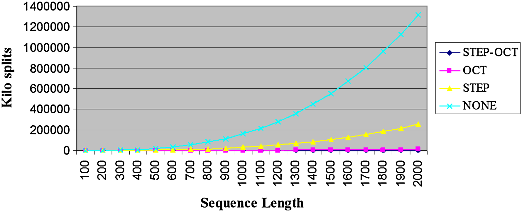
Average examined split points per sequence length. The NONE curve corresponds to the case where no sparsification was applies. The STEP curve corresponds to the case where split points were examined only if the induced prefix satisfies the STEP criteria. The OCT curve corresponds to the case where split points were examined only if the induced suffix satisfies the OCT criteria. The STEP-OCT curve corresponds to the case where split points were examined only if the induced prefix satisfies the STEP criteria, and the induced suffix satisfies the OCT criteria. Since the STEP-OCT curve is of a significantly lower magnitude with respect to the NONE curve, we refer the reader to Figure 6 in which only the STEP-OCT and OCT curves are shown.

FIG. 6.

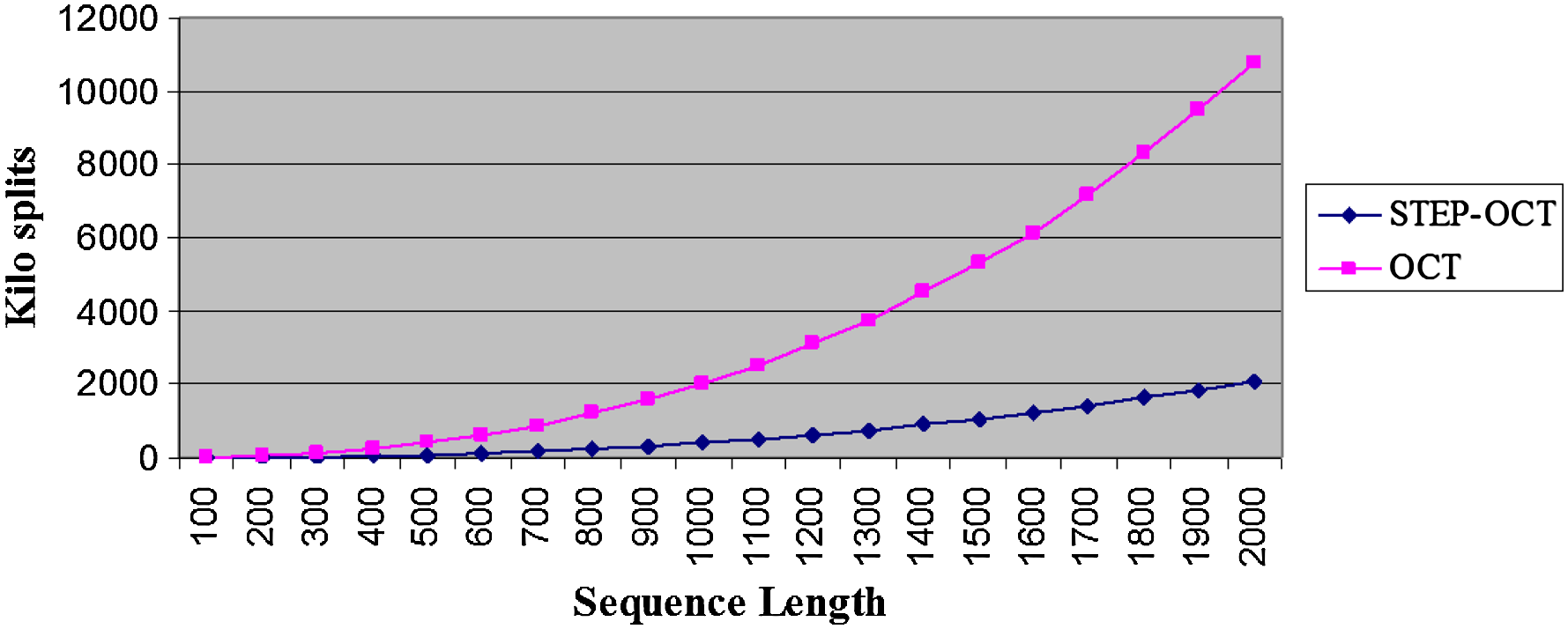
Average examined split points per sequence length. The figure shows only the OCT and STEPOCT curves of Figure 5.

FIG. 7.

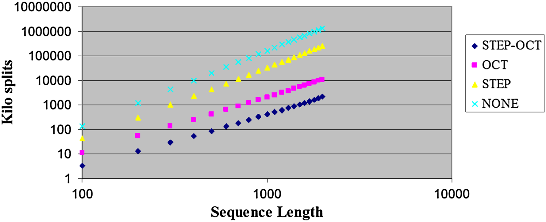
Average examined split points per sequence length. A log-log scale representation of Figure 5.

Footnotes

Acknowledgments

We are grateful to Mirela Andronescu for her kind help in providing information and pointing us to relevant data, and to Holger Hoos and the anonymous reviewers for their helpful comments. The research of S.Z. and M.Z.-U. was supported by ISF grant 478/10.

Disclosure Statement

No competing financial interests exist.

1

Some scoring models also utilize homology information with respect to two or more sequences. Such comparative approaches are beyond the scope of this work.

2

In models whose scores correspond to free energies, the score optimization is traditionally formulated as a minimization problem. This formulation can be easily transformed to the maximization formulation that is used here.

3

In this sense, internal-loop lengths are not restricted here as done in some other models, where arbitrary-length internal-loops are scored with respect to their unpaired bases and terminating base-pairs, and length-depended corrections are added to the scores of relatively “short” loops.

4

This is a common setting in online learning algorithms; for a justification based on an analysis of stochastic-gradient-descent optimization, see Zhang (2004).

References

Andronescu

2008. Computational approaches for RNA energy parameter estimation[Ph.D. dissertation]University of British Columbia: Vancouver, Canada.

Andronescu

, Bereg

, Hoos

H.H.

et al. 2008. RNA STRAND: the RNA secondary structure and statistical analysis database. BMC Bioinform., 9:340.

Andronescu

, Condon

, Hoos

et al. 2010. Computational approaches for RNA energy parameter estimation. RNA, 16:2304–2318.

Andronescu

, Condon

, Hoos

H.H.

et al. 2007. Efficient parameter estimation for RNA secondary structure prediction. Bioinformatics, 23:i19.

Backofen

, Tsur

, Zakov

et al. 2011. Sparse RNA folding: time and space efficient algorithms. J. Discr. Algo-rithms, 9:12–31.

Chiang

, Knight

, Wang

2009. 11,001 new features for statistical machine translation. Proc. HLT-NAACL 2009, 218–226.

Collins

2002. Discriminative training methods for hidden Markov models: theory and experiments with perceptron algorithms. Proc. ACL-02 Conf. Empirical Methods Natural Lang. Processing, 1–8.

Crammer

, Dekel

, Keshet

et al. 2006. Online passive-aggressive algorithms. J. Mach. Learn. Res., 7:585.

Darty

, Denise

, Ponty

2009. VARNA: interactive drawing and editing of the RNA secondary structure. Bioinformatics, 25:1974–1975.

10.

C.B.

, Foo

C.S.

, Ng

A.Y.

2007. Efficient multiple hyperparameter learning for log-linear models. Neural Inform. Process. Syst., 21.

11.

C.B.

, Woods

D.A.

, Batzoglou

2006. CONTRAfold: RNA secondary structure prediction without physics-based models. Bioinformatics, 22:e90–e98.

12.

Dowell

R.D.

, Eddy

S.R.

2004. Evaluation of several lightweight stochastic context-free grammars for RNA secondary structure prediction. BMC Bioinform., 5:71.

13.

Durbin

, Eddy

, Krogh

et al. 1998. Biological sequence Analysis: Probabilistic Models of Proteins and Nucleic Acids. Cambridge University Press: New York.

14.

Eddy

S.R.

2001. Non–coding RNA genes and the modern RNA world. Nat. Rev. Genet., 2:919–929.

15.

Eddy

S.R.

, Durbin

1994. RNA sequence analysis using covariance models. Nucleic Acids Res., 22:2079.

16.

Freund

, Schapire

R.E.

1999. Large margin classification using the perceptron algorithm. Mach. Learn., 37:277–296.

17.

Griffiths-Jones

, Moxon

, Marshall

et al. 2005. Rfam: annotating non-coding RNAs in complete genomes. Nucleic Acids Res., 33:D121.

18.

Hofacker

I.L.

, Fontana

, Stadler

P.F.

et al. 2002. Vienna RNA package. www.tbi.univie.ac.at/ivo/RNA. 2011 August 15.

19.

Hofacker

I.L.

, Stadler

P.F.

, Stocsits

R.R.

2004. Conserved RNA secondary structures in viral genomes: a survey. Bioinformatics, 20:1495.

20.

Kloc

, Zearfoss

N.R.

, Etkin

L.D.

2002. Mechanisms of subcellular mRNA localization. Cell, 108:533–544.

21.

Mandal

, Breaker

R.R.

2004. Gene regulation by riboswitches. Cell, 6:451–463.

22.

Mathews

D.H.

, Burkard

M.E.

, Freier

S.M.

et al. 1999a. Predicting oligonucleotide affinity to nucleic acid target. RNA, 5:1458.

23.

Mathews

D.H.

, Sabina

, Zuker

et al. 1999b. Expanded sequence dependence of thermodynamic parameters improves prediction of RNA secondary structure. J. Mol. Biol., 288:911–940.

24.

Mattick

J.S.

2004. RNA regulation: a new genetics? Pharmacogenomics J, 4:9–16.

25.

McDonald

, Crammer

, Pereira

2005. Online large-margin training of dependency parsers. Proc. ACL 2009 Conf.

26.

Möhl

, Salari

, Will

et al. 2010. Sparsification of RNA structure prediction including pseudoknots. Proc. WABI 2010, 40.

27.

Nussinov

, Jacobson

A.B.

1980. Fast algorithm for predicting the secondary structure of single-stranded RNA. Proc. Natl. Acad. Sci. USA, 77:6309–6313.

28.

Sakakibara

, Brown

, Hughey

et al. 1994. Stochastic context-free grammers for tRNA modeling. Nucleic Acids Res., 22:5112.

29.

Salari

, Möhl

, Will

et al. 2010. Time and space efficient RNA-RNA interaction prediction via sparse folding. Proc. RECOMB 2010, 473–490.

30.

Tinoco

, Borer

P.N.

, Dengler

et al. 1973. Improved estimation of secondary structure in ribonucleic acids. Nat. New Biol., 246:40–41.

31.

Tinoco

, Uhlenbeck

O.C.

, Levine

M.D.

1971. Estimation of secondary structure in ribonucleic acids. Nature, 230:362–367.

32.

Washietl

, Hofacker

I.L.

, Lukasser

et al. 2005. Mapping of conserved RNA secondary structures predicts thousands of functional noncoding RNAs in the human genome. Nat. Biotechnol., 23:1383–1390.

33.

Watanabe

, Asahara

, Matsumoto

2010. A structured model for joint learning of argument roles and predicate senses. Proc. ACL 2010 Conf., 98–102.

34.

Wexler

, Zilberstein

, Ziv-Ukelson

2007. A study of accessible motifs and RNA folding complexity. J. Comput. Biol., 14:856–872.

35.

Zhang

2004. Solving large-scale linear prediction problems using stochastic gradient descent algorithms. Proc. ICML 2004.

36.

Ziv-Ukelson

, Gat-Viks

, Wexler

et al. 2008. A faster algorithm for RNA co-folding. Algorithms Bioinform., 174–185.

37.

Zuker

1989. Computer prediction of RNA structure. Methods Enzymol., 180:262–288.

38.

Zuker

2003. Mfold web server for nucleic acid folding and hybridization prediction. Nucleic Acids Res., 13:3406–3415.

39.

Zuker

, Stiegler

1981. Optimal computer folding of large RNA sequences using thermodynamics and auxiliary information. Nucleic Acids Res., 9:133–148.