




Abstract
Abstract
Bacteria are the unseen majority on our planet, with millions of species and comprising most of the living protoplasm. We propose a novel approach for reconstruction of the composition of an unknown mixture of bacteria using a single Sanger-sequencing reaction of the mixture. Our method is based on compressive sensing theory, which deals with reconstruction of a sparse signal using a small number of measurements. Utilizing the fact that in many cases each bacterial community is comprised of a small subset of all known bacterial species, we show the feasibility of this approach for determining the composition of a bacterial mixture. Using simulations, we show that sequencing a few hundred base-pairs of the 16S rRNA gene sequence may provide enough information for reconstruction of mixtures containing tens of species, out of tens of thousands, even in the presence of realistic measurement noise. Finally, we show initial promising results when applying our method for the reconstruction of a toy experimental mixture with five species. Our approach may have a potential for a simple and efficient way for identifying bacterial species compositions in biological samples. All supplementary data and the MATLAB code are available at www.broadinstitute.org/∼orzuk/publications/BCS/.
1. Introduction
Identification of the bacteria present in a given sample is not simple, and technical limitations impede large scale quantitative surveys of bacterial community compositions. Since the vast majority of bacterial species are non-amenable to standard laboratory cultivation procedures (Amann et al., 1995), culture-independent methods are needed. The golden standard of microbial population analysis has been cloning and direct Sanger sequencing of the ribosomal 16S subunit gene (16S rRNA) (Hugenholtz, 2002). However, since each 16S rRNA sequence is sampled randomly from the mixture, the sensitivity of this method is determined by the number of sequencing reactions, and therefore tens to hundreds of sequencing reactions are required for each sample analyzed. A modification of this method for identification of small mixtures of bacteria using a single Sanger sequence has been suggested (Kommedal et al., 2008) and showed promising results when reconstructing mixtures of 2–3 bacteria from a given database of ∼260 human pathogen sequences.
Recently, DNA microarray-based methods (Gentry et al., 2006) and identification via next generation sequencing (Hamady and Knight, 2009) have been used for bacterial community reconstruction. In microarray-based methods, such as the Affymetrix PhyloChip platform (Brodie et al., 2007), the sample 16S rRNA is hybridized with short probes aimed at identification of known microbes at various taxonomy levels. While being more sensitive and cheaper than standard cloning and sequencing techniques, each bacterial mixture sample still needs to be hybridized against a microarray, thus the cost of such methods limit their use for wide-scale studies. Methods based on next generation sequencing obtain a very large number of reads of a short hyper-variable region of the 16S rRNA gene (Armougom and Raoult, 2008; Dethlefsen et al., 2008; Hamady et al., 2008). Usage of such methods, combined with DNA barcoding, enables high-throughput identification of bacterial communities, and can potentially detect species present at very low frequencies. However, since such sequencing methods are limited to relatively short read lengths (typically a few dozens and at most a few hundred bases in each sequence), species identification is not straightforward. In practice, identification using current methods is nonunique and limited in resolution, with reliable identification typically up to the genus level (Huse et al., 2008). Improving resolution depends on obtaining longer read lengths, which is currently technologically challenging, and/or developing novel analytical methods which utilize the (possibly limited) information from each read to allow in aggregate a better separation between the species.
In this work we suggest a novel experimental and computational approach for sequencing-based profiling of bacterial communities (Fig. 1). We demonstrate our method using a single Sanger sequencing reaction for a bacterial mixture, which results in a linear combination of the constituent sequences. Using this mixed chromatogram as linear constraints, the sequences which constitute the original mixture are selected using a Compressed Sensing (
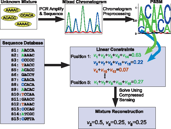
Schematics of the proposed BCS reconstruction method. The 16S rRNA gene is PCR-amplified from the mixture and then subjected to Sanger sequencing. The resulting chromatogram is preprocessed to create the Position Specific Score Matrix (PSSM). For each sequence position, four linear mixture equations are derived from the 16S rRNA sequence database, with vi denoting the frequency of sequence i in the mixture, and the frequency sum taken from the experimental PSSM. These linear constraints are used as input to the
Compressed Sensing (
The classical
where
In this article, we show an efficient application of a single Sanger-sequencing for bacterial communities reconstruction using
The proposed Bacterial Compressed Sensing (
2. Methods
2.1. The BCS algorithm
In the Bacterial Community Reconstruction Problem, we are given a bacterial mixture of unknown composition. In addition, we have at hand a database of the orthologous genomic sequences for a specific known gene, which is assumed to be present in a large number of bacterial species (in our case, the gene used was the 16S rRNA gene). Our purpose is to reconstruct the identity of species present in the mixture, as well as their frequencies, where the assumption is that the sequences for the gene in all or the vast majority of species present in the mixture are available in the database. The input to the reconstruction algorithm is the measured Sanger sequence of the gene in the mixture (Fig. 1). Since Sanger sequencing proceeds independently for each DNA molecule present in the sample, the sequence chromatogram of the mixture corresponds to the linear combination of the constituent sequences, where the linear coefficients are proportional to the abundance of each species in the mixture.
Let N be the number of known bacterial species present in our database. Each bacterial population is characterized by a vector
We represent the results of the mixture Sanger sequencing as a 4 × k Position-specific-Score-Matrix (PSSM)
where
Each position in the mixed sequence gives information about the bacterial composition of the mixture. For example, if at a certain position j, the frequency aj of “A” in the mixed sequence is 0, and assuming no measurement noise is present, it follows that all bacteria which have “A” at the j'th position of their orthologous gene are not present in the mixture, and their corresponding frequencies in the solution vector must be zero. More generally, the frequency of each nucleotide at a given position j gives a linear constraint on the mixture:
and similarly for the nucleotides “C”, “G”, and “T”. We next define the k × N mixture matrix A for the nucleotide “A”,
and similarly for the nucleotides “C”, “G”, and “T”. The constraints given by the sequencing reaction can therefore be expressed in matrix form as:
The crucial assumption we make in order to cope with the insufficiency of information is the sparsity of the vector
which is a convex optimization problem whose solution can be obtained in polynomial time. The above formulation requires our measurements to be precisely equal to their expected value based on the species frequency and the linearity assumption for the measured chromatogram. This description ignores the effects of noise, which is typically encountered in practice, on the reconstruction. Measurements of the signal mixtures suffer from various types of noise and biases. Fortunately, the
This problem represents a more general form of eq. (6) and accounts for noise in the measurement process. This is utilized by insertion of an ℓ2 quadratic error term. The parameter τ determines the relative weight of the error term vs. the sparsity promoting term, with higher levels of τ leading to a sparser solution. Many algorithms which enable an efficient solution of problem (7) are available, and we have chosen the widely used GPSR algorithm (Figueiredo et al., 2007). The error tolerance parameter was set to τ = 10 for the simulated mixture reconstruction, and τ = 100 for the reconstruction of the experimental mixture. These values achieved a rather sparse solution in most cases (a few species reconstructed with frequencies above zero), while still giving a good sensitivity—our ability to identify correctly species present in the mixture is not compromised significantly. The performance of the algorithm was quite robust to the specific value of τ used, and therefore further optimization of the results by fine tuning τ was not followed in this study.
2.2. Ribosomal DNA database
16S rRNA gene sequences were obtained from grenegenes (greengenes.lbl.gov) using database version 06-2007 (DeSantis et al., 2006), which contains approximately 136, 000 chimera checked full-length sequences. Sequences were reverse complemented and aligned with primer 1510R (Gao et al., 2007), resulting in approximately 42,000 sequences matching the primer sequence (with up to six mismatches with the primer). Out of this set, sequences with up to two base-pair difference with another sequence in the database were removed, resulting in N = 18, 747 unique sequences which were used in this study. This last step was used for two purposes: first, to unite closely related species and enable a coarser identification of species in the mixture (since the information provided by the sequencing may not suffice to distinguish between very close species), and second, to reduce input size to the GPSR algorithm, thus making the
We manually added the sequence of Enterococcus faecalis (ATCC no. 19433) to the unique sequences list, as it was used in the experimental mixture but did not appear in the database (closest database species has 32 different positions).
2.3. Experimental mixture reconstruction
2.3.1. Sample preparation
We used the following strains for the experimental reconstruction: Escherichia coli W3110, Vibrio fischeri, Staphylococcus epidermidis (ATCC no. 12228), Enterococcus faecalis (ATCC no. 19433), and Photobacterium leiognathi. We obtained the 16S rRNA gene from each bacterial strain by boiling for one minute followed by 40 cycles of PCR amplification. Primers used for the PCR were the universal primers 8F and 1510R (Gao et al., 2007), amplifying positions 8–1513 of the E. coli 16S rRNA,
For mixture preparation and sequencing, we mixed together equal amounts of DNA from each bacterial 16S rRNA gene, and then sequenced them using an ABI3730 DNA Analyzer (Applied Biosystems, USA) with the 1510R primer.
2.3.2. Preprocessing steps
The input to the
We therefore opted for a slightly different approach for chromatogram preprocessing, which does not depend on identifying the peak for each nucleotide. Rather, we bin the chromatogram into constant sized bins, and use the total intensity of each of the four nucleotides in each bin to construct the PSSM used as input to the
Figure 10 below shows the inherent variation in chromatogram peak distances and heights, a substantial part of it is due to local sequence context, while Figure 11 below shows that considering these local sequence effects significantly improves our estimation of chromatogram peak locations and heights. The database of predicted PSSMs is then used to construct the mixing matrices A, C, G, T participating in the
3. Results
3.1. Simulation results
In order to asses the performance of the proposed
A sample of a random mixture of 10 sequences, and a part of the corresponding mixed sequence PSSM, are shown in Figure 2A,B, respectively. Results of the
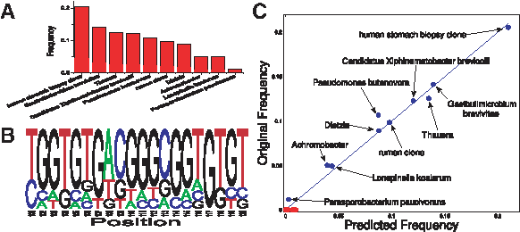
Sample reconstruction of a simulated mixture.
3.1.1. Coherence of database sequences
As detailed in the previous sections, the
It has previously been shown (Ben-Haim et al., 2010, Tropp, 2006) that a computationally feasible method for assessing the information content of the mixing matrix is the mutual coherence, defined as the maximal coherence (inner product) between two columns of the mixing matrix. We therefore analyzed the empirical coherence distribution of sequences present in the current database. Even though the sequences are orthologous and thus quite similar, insertions and deletions came to our aid, as they bring similar sequences to being out of phase (e.g., even a deletion of a single base from a sequence, reduces its correlation with a copy of itself from one to a number typically much lower).
The distribution of coherence values for random pairs of database species is shown in Figure 3. While most correlations are centered around 0.25, there exists a small fraction of highly correlated sequences, with 0.005 of the sequence pairs showing a correlation above 0.8, and a maximal correlation value of 0.998. This high mutual coherence value places a limit on the reconstruction performance in the worst case, when such a sequence is present in the mixture. Since the database contains another highly similar sequence, distinguishing between these two is very difficult, and therefore the
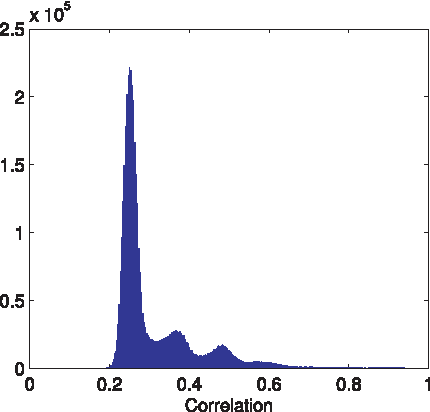
Coherence distribution of the 16S rRNA sequences. Coherence (inner product) of 107 16S rRNA vector pairs chosen randomly from the sequence database (∼5.7% of all possible pairs). As each column of the mixture matrix is a binary vector with 1/4 of the coordinates being one, the dot product between two randomly generated vectors is expected to be ∼0.25. While most 16S rRNA database pairs exhibit a coherence around 0.25, many pairs exhibit significantly higher correlations, with a few (∼0.5%) even exceeding 0.8 (see inset).
3.1.2. Effect of sequence length
To determine the typical sequence length required for reconstruction, we tested the
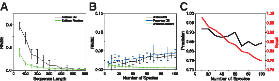
Reconstruction of simulated mixtures.
In order to asses the effect of similarites between the database sequences (which leads to high coherence of the mixing matrix columns) on the performance of the
3.1.3. Effect of number of species
For a fixed value of k = 500 nucleotides per sequencing run, the effect of the number of species present in the mixture on reconstruction performance is shown in Figure 4B,C. Even on a mixture of 100 species, the reconstruction showed an average RMSE less than 0.04, with the highest false positive reconstructed frequency (i.e., frequency for species not present in the original mixture) being less than 0.01. Using a minimal frequency threshold of 0.0025 for calling a species present in the reconstruction, the
The frequencies of species in a biologically relevant mixture need not be uniformly distributed. For example, the frequency of species found on the human skin (Gao et al., 2007) were shown to resemble a power-law distribution. We therefore tested the performance of the
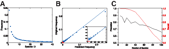
Sample reconstruction of a power-law mixture.
3.1.4. Effect of noise on BCS solution
Experimental Sanger sequencing chromatograms contain inherent noise, and we cannot expect to obtain exact measurements in practice. We therefore turned to study the effect of noise on the accuracy of the
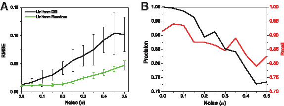
Effect of noise on reconstruction.
Using a noise standard deviation of σ = 0.15 (which is the approximate experimental noise level) and sequencing 500 nucleotides, the reconstruction performance as a function of the number of species in the mixture is shown in Figure 7. Under this noise level, the
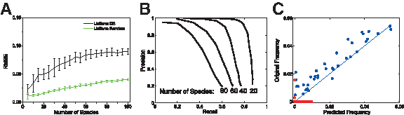
Reconstruction with experimental noise level.
3.2. Reconstruction of an experimental mixture
While these simulations show promising results, they are based on correctly converting the experimentally measured chromatogram to the PSSM used as input to the
We tested the feasibility of the

Reconstruction of an experimental mixture.
Results of the reconstruction are shown in Figure 8C. The algorithm successfully identifies three of the five bacteria (Vibrio fischeri, Enterococcus faecalis, and Photobacterium leiognathi). Out of the two remaining strains, one (Staphylococcus epidermidis) is identified at the genus level, and the other (Escherichia coli) is mistakenly identified as Salmonella enterica. While Escherichia coli and Salmonella enterica show a sequence difference in 33 bases over the PCR amplified region, only two bases are different in the region used for the
4. Discussion
In this work, we have proposed a framework for identifying and quantifying the presence of bacterial species in a given population using information from a single sequencing reaction. Simulation results with noise levels comparable to the measured noise in chromatograms obtained experimentally for real sequence indicate that our method can reconstruct mixtures of tens of species. When not enough information is present in the sequence (e.g., when the number of sequences present in the mixture is large), performance of the reconstruction algorithm decays gracefully, and still retains detection of the prominent species.
In order to test the applicability of the
The amount of information needed for identifying the species present in the mixture is logarithmic in the database size (Candes, 2006; Donoho, 2006a), as long as the number of the species present in the mixture is kept constant. Therefore, a single sequencing reaction with hundreds of bases may in principle provide sufficient information for unique reconstruction even when the database contains millions of different sequences. Compressed Sensing enables the use of such information redundancy through the use of linear mixtures of the sample. However, coherence between the columns of the reconstruction matrix may hinder the reconstruction performance. The mixtures are dictated by the sequences in the database, which are exhibit a complicated dependence structure resulting from the phylogenetic relationships of both the species and the 16S rRNA gene. Since the mixing matrix is built using each sequence in the database separately, our method does not rely on correct alignment of the database sequences. While two sequences which differ in a few nucleotides have high coherence and clearly do not contribute to RIP, even a single insertion or deletion completely brings the two sequences to being “out of phase,” thus making it easier to distinguish between them using
While limited to the identification of species with known 16S rRNA sequences, the
5. Appendix
A: Chromatogram Preprocessing
The purpose of the chromatogram preprocessing scheme is to convert the raw measured chromatogram data to a PSSM representing the frequency of each base at each position along the sequence in the mixture (Fig. 9A). We provide below a formal algorithm sketch for this step, followed by a more detailed description:

Preprocessing steps.
Chromatogram preprocessing
The input to the chromatogram preprocessing is the measured chromatogram, consisting of four fluorescent trace vectors a, c, g, t, where for example a p represents the signal intensity for nucleotide “A” at the p's position along the chromatogram, where each position is represented by one pixel in the chromatogram image. The value p corresponds roughly to the timing of the sequencing reaction, with a resolution of approximately a dozen points per nucleotide, thus p runs from 1 to ∼12k (a few thousand points in a typical chromatogram—for example, 6900 points in the experimental chromatogram described in Section 3, corresponding to approximately 575 base-pairs).
In a typical Sanger sequencing reaction, the chromatogram peak heights decrease as the position p becomes higher (nucleotides further in the sequence which were sequenced later in the sequencing reaction) due to depletion of the dideoxynucleotides. To overcome this long-scale decrease in signal amplitude, prior to the binning step, the amplitude at each position was normalized by division with average total peak height in a ∼50 base-pair (bp) region around each position (see step 1 in the algorithm description below).
The resulting vectors after the normalization step are binned into constant sized bins (12 pixels per bin), and the sum of intensity values of each bin is computed for the four different nucleotides. Then, we take square root of this sum for the four different nucleotides for the i'th bin as the i'th column in the output 4 × k PSSM. The square root is used rather than the sum as this was shown to decrease the effect of large outliers. The resulting 4 × k PSSM is used as input to the
B: Database Preprocessing
The purpose of the Database Preprocessing scheme is to produce predicted PSSMs for all 16S rRNA sequences in the database (Fig. 9B). For each sequence Si in the database sequences we compute a PSSM Pi = (
We use a generative model-based approach for simulating the measured PSSMs obtained from an (hypothetical) measured chromatogram for each sequence in the database. The model generates, as an intermediate stage, a predicted chromatogram for the input sequence. This chromatogram is then further processed to obtain the predicted PSSM. The model captures the relations between the sequence of nucleotides comprising a DNA molecule and the chromatogram charts obtained when sequencing such a molecule. The main factor affecting the chromatogram shape is local-sequence context, which we modeled by a 5th order Markov Chain. We fitted the model parameters in a preliminary step by using a training set of sequences with experimentally available chromatograms. We describe this preliminary step in the next section. Next, in the Database PSSMs Generation Step Section, we describe the database preprocessing step performed once the model parameters are fully specified.
Preliminary step: Compute local-sequence adjusted chromatogram statistics
The preliminary step fits model parameters representing context-specific peak height and width, as well as a sequence-position dependent correction factor β used to model variation in peak position. We give a formal algorithm sketch followed by a detailed description:
Compute local-adjusted chromatogram statistics
In the course of the Sanger sequencing process, both the polymerase specificity for incorporating deoxynucleotides over dideoxynucleotides and the fragment mobility depend on sequence local to the incorporation point. Therefore for each nucleotide in the DNA fragment being sequenced, its corresponding chromatogram peak height and position are affected by the preceding nucleotides (Lipshutz et al., 1994). In order to predict and correct for the effect of local sequence context on the resulting chromatogram, we collected statistics from a training set S′ of 1000 sequencing runs performed on an ABI3730 machine. Runs were randomly selected from experiments submitted for sequencing in the Weizmann Institute sequencing unit by various labs. The average length of the runs was approximately 800 base-pairs, providing in total chromatogram statistics for ∼800,000 nucleotides. Chromatogram heights hi,j were normalized to overcome the long-scale amplitude decrease (as described in Appendix A).
We have modeled the local sequence context by looking at the 5 nucleotides preceding each nucleotide, giving us 46 = 4096 different unique 6-mers, each representing a possible nucleotide and the five nucleotides preceding it. For each unique 6-mer, the fitting step searches for all of its occurrences in S′, and averages the peak height and position data of the last nucleotide over all such occurrences in S′. We have used 6-mers as this gives the maximal context length for which we had sufficient statistics to collect for each 6-mer. Approximately 200 instances were available per 6-mer on average, with a minimal number of 16 instances for one 6-mer (it is possible that a smaller local sequence context is sufficient for accurate prediction of chromatogram heights).
The resulting final peak height and distance tables H and D, respectively, each of size 4096(= 46), are available at www.broadinstitute.org/norzuk/publications/BCS/. While the average height and position were 1 (as was ensured by our normalizations), there was significant variability in height and position according to sequence context, with height values H typically in the range of ∼0.5–1.3 and position values P in the range of ∼0.8–1.2 (Fig. 10). We observed an additional sequence-independent change in peak-peak distance in the chromatograms studied, where distance between consecutive peaks increases as we move further along the chromatogram. We accounted for this by fitting an additional linear model based only on the nucleotide position along the sequence according to eq. (13), giving an additional parameter of β = 0.00036 representing increase in peak-peak distance with each position - we used this parameter later to predict the resulting chromatograms (see eq. (15) in Algorithm 3).
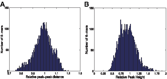
Local-sequence effect on chromatogram peak height and position.
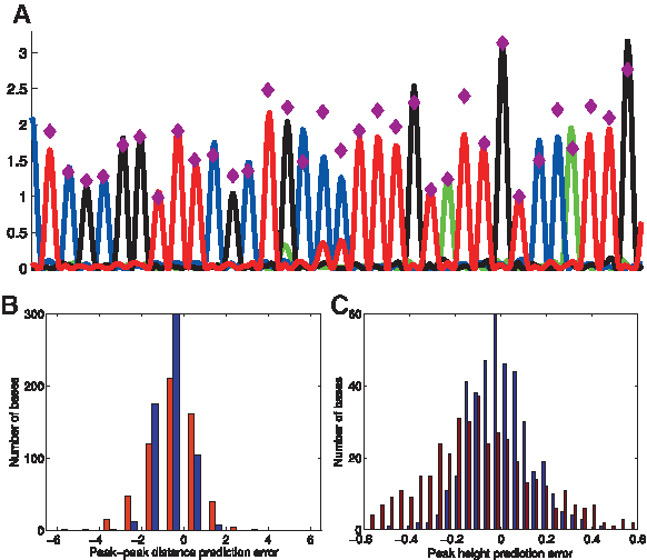
Correcting for local sequence effects on chromatogram peak heights and positions.
Database PSSMs Generation step: Generate a database of predicted PSSMs
This step generates predicted PSSMs for the N sequences in the 16S rRNA database S. It uses the model parameters from the training set described in the previous Section. The sequence input S and model parameters are used to determine peak heights and positions and thus compute a set of N chromatograms of the form (a, c, g, t), one for each 16S rRNA gene sequence in S. We then further process these chromatograms to get predicted PSSMs. This step is illustrated in Figure 9B. We give the details next in Algorithm 3:
Compute PSSM from chromatogram
The database preprocessing step was applied for a database sequence matrix S, comprised of 18, 747 unique 16S rRNA gene sequences of average length 1,480 bases (see Section 2.2). The output is a set of PSSMs Pi = (
We generated a chromatogram trace for a given 16S rRNA gene sequence by modeling each peak as a Gaussian centered at the peak position and with height equal to the peak height. The widths of the chromatogram Gaussian peaks were approximated using a constant peak width obtained by setting c = 0.4.
Each fi,j was evaluated for x values equally spaced in the entire sequence range [0,k], but has a non-negligible contribution to the entire chromatogram only in the vicinity of the nucleotide position bi,j, as is ensured by the Gaussian decay. A resolution of 1/12 was used as it corresponds roughly to the number of pixels available for a single nucleotide in real chromatograms. A chromatogram was generated for each 16S rRNA gene sequence by summing the values of obtained fi,j over all nucleotides.
Alignment of predicted and measured chromatograms
Sanger-sequencing chromatograms display an initial region (∼100 bases), which is highly noisy and therefore unusable. We are therefore faced with the problem of correctly aligning the initial bin position in the measured chromatogram and the bin positions of the predicted chromatograms. This was solved by trying the
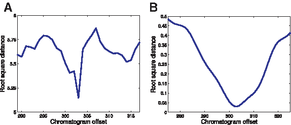
Determination of chromatogram offset.
Footnotes
Acknowledgments
We thank Amit Singer, Yonina Eldar, Gidi Lazovski, and Noam Shental for useful discussions, Eytan Domany for critical reading of the manuscript, Joel Stavans for supporting this research, and Chaime Priluski for assistance with chromatogram peak prediction data.
Disclosure Statement
No competing financial interests exist.