In a recent article, Behrens and Vingron (J. Comput. Biol. 17/12, 2010) compute waiting times for k-mers to appear during DNA evolution under the assumption that the considered k-mers do not occur in the initial DNA sequence, an issue arising when studying the evolution of regulatory DNA sequences with regard to transcription factor (TF) binding site emergence. The mathematical analysis underlying their computation assumes that occurrences of words under interest do not overlap. We relax here this assumption by use of an automata approach. In an alphabet of size 4 like the DNA alphabet, most words have no or a low autocorrelation; therefore, globally, our results confirm those of Behrens and Vingron. The outcome is quite different when considering highly autocorrelated k-mers; in this case, the autocorrelation pushes down the probability of occurrence of these k-mers at generation 1 and, consequently, increases the waiting time for apparition of these k-mers up to 40%. An analysis of existing TF binding sites unveils a significant proportion of k-mers exhibiting autocorrelation. Thus, our computations based on automata greatly improve the accuracy of predicting waiting times for the emergence of TF binding sites to appear during DNA evolution. We do the computation in the Bernoulli or M0 model; computations in the M1 model, a Markov model of order 1, are more costly in terms of time and memory but should produce similar results. While Behrens and Vingron considered specifically promoters of length 1000, we extend the results to promoters of any size; we exhibit the property that the probability that a k-mer occurs at generation time 1 while being absent at time 0 behaves linearly with respect to the length of the promoter, which induces a hyperbolic behaviour of the waiting time of any k-mer with respect to the length of the promoter. The C code is available at www.lipn.univ-paris13.fr/∼nicodeme/.
1. Introduction
The expression of genes is subject to strong regulation. The key concept of transcriptional gene regulation is the binding of proteins, so called transcription factors (TFs), to TF binding sites. These TF binding sites are typically short stretches of DNA, many of which are only approximately 5–8 bp long (Wray et al., 2003). Usually, these TF binding sites are located in a region around 1000 bp upstream of the gene they regulate, the so-called promoter. Thus, the occurrence of particular k-mers in these promoter regions has a high impact on modulating transcription. There have been several experimental studies employing ChIP-chip or ChIP-seq technology showing that promoters are rapidly evolving regions that change over short evolutionary time scales (Odom et al., 2007; Schmidt et al., 2010; Kunarso et al., 2010). In a recent review, Dowell (2010) summarizes all these experimental findings and concludes that most TF binding events are species-specific and that gene regulation is a highly dynamic evolutionary process. Many of these changes in TF binding, if not necessarily all, can be explained by gains and losses of TF binding sites.
Several theoretical studies have tried to give a probabilistic explanation for the speed of changes in transcriptional gene regulation (Stone and Wray, 2001; Durrett and Schmidt, 2007). Behrens and Vingron (2010) infer how long one has to wait until a given TF binding site emerges at random in a promoter sequence. Using two different probabilistic models (a Bernoulli model denoted by M0 and a neighbor-dependent model M1) and estimating evolutionary substitution rates based on multiple species promoter alignments for the three species Homo sapiens, Pan troglodytes, and Macaca mulatta, they compute the expected waiting time for every k-mer, k ranging from 5 to 10, until it appears in a human promoter. They conclude that the waiting time for a TF binding site is highly determined by its composition and that indeed TF binding sites can appear rapidly (i.e., in a time span below the speciation time of human and chimp).
However, in their approach, Behrens and Vingron (2010) rely on the assumption that if a k-mer of interest appears more than once in a promoter sequence, it does not overlap with itself. This particularly affects the waiting times for highly autocorrelated words like e.g. AAAAA or CTCTCTCTCT. Using automata, we can relax this assumption and, thus, more accurately compute the expected waiting times until appearance for every k-mer, k ranging from 5 to 10, in a promoter of length 1000 bp. This automaton approach can be applied both for models M0 and M1. However, for the ease of exposition, in this article we will focus on the Bernoulli model M0.
This article is structured as follows. In Section 2, we describe model M0, state results from Behrens and Vingron (2010) that we rely on, and recall how Behrens and Vingron (2010) have estimated model M0 parameters based on human, chimp, and macaque promoter alignments. In Section 3 we present our new approach of computing waiting times using automata theory; we provide in this section, a web-pointer to the program used to perform these computations. Section 4 compares the results of computing waiting times for k-mers to appear in a promoter of length 1 kb according to Behrens and Vingron (2010) and to our new automaton approach. For both computations, we employ the same model parameters estimations that have been already used in Behrens and Vingron (2010); we also explain in this section the biological impact of our findings and show that autocorrelation matters in the context of TF binding site emergence. Section 5 exhibits the first order linear behaviour of the probability of evolution to a k-mer from generation time 0 to time 1 for specific examples; the observed phenomena is however general, as proved in Nicodème (2011). We provide in this section a web-pointer to a database containing the waiting times of all k-mers for k from 5 to 10 and for promoter lengths n = 1000 and n = 2000. Section 6 will conclude the article with some summarizing remarks.
2. Model M0 and Expected Waiting Times
Throughout the article, we assume that promoter sequences evolve according to model M0, which has been described by Behrens and Vingron (2010).
Model M0
Given an alphabet
\documentclass{aastex}
\usepackage{amsbsy}
\usepackage{amsfonts}
\usepackage{amssymb}
\usepackage{bm}
\usepackage{mathrsfs}
\usepackage{pifont}
\usepackage{stmaryrd}
\usepackage{textcomp}
\usepackage{portland, xspace}
\usepackage{amsmath, amsxtra}
\pagestyle{empty}
\DeclareMathSizes {10} {9} {7} {6}
\begin{document}
$${\cal A} = \{{\rm A , C , G , T} \} $$\end{document}, let
\documentclass{aastex}
\usepackage{amsbsy}
\usepackage{amsfonts}
\usepackage{amssymb}
\usepackage{bm}
\usepackage{mathrsfs}
\usepackage{pifont}
\usepackage{stmaryrd}
\usepackage{textcomp}
\usepackage{portland, xspace}
\usepackage{amsmath, amsxtra}
\pagestyle{empty}
\DeclareMathSizes {10} {9} {7} {6}
\begin{document}
$$S ( 0 ) = ( S_1 ( 0 ) , \ldots , S_n ( 0 ) )$$\end{document} denote the initial promoter sequence of length n taking values in this alphabet. We assume that the letters in S(0) are independent and identically distributed with ν(x) : = Pr(S1(0) = x). Let the time evolution
\documentclass{aastex}
\usepackage{amsbsy}
\usepackage{amsfonts}
\usepackage{amssymb}
\usepackage{bm}
\usepackage{mathrsfs}
\usepackage{pifont}
\usepackage{stmaryrd}
\usepackage{textcomp}
\usepackage{portland, xspace}
\usepackage{amsmath, amsxtra}
\pagestyle{empty}
\DeclareMathSizes {10} {9} {7} {6}
\begin{document}
$$( S ( t ) ) _{t \geq 0}$$\end{document} of the promoter sequence be governed by the 4 × 4 infinitesimal rate matrix
\documentclass{aastex}
\usepackage{amsbsy}
\usepackage{amsfonts}
\usepackage{amssymb}
\usepackage{bm}
\usepackage{mathrsfs}
\usepackage{pifont}
\usepackage{stmaryrd}
\usepackage{textcomp}
\usepackage{portland, xspace}
\usepackage{amsmath, amsxtra}
\pagestyle{empty}
\DeclareMathSizes {10} {9} {7} {6}
\begin{document}
$${\mathbb Q} = ( r_{\alpha , \beta} ) _{\alpha , \beta \in {\cal A}}$$\end{document}. According to the general reverse complement symmetric substitution model, we assume that the nucleotides evolve independently from each other and that rA,T = rT,A, rC,G = rG,C, rA,C = rT,G, rC,A = rG,T, rA,G = rT,C and rG,A = rC,T (Duret and Arndt, 2008). Thus, there are six free parameters. The matrix
\documentclass{aastex}
\usepackage{amsbsy}
\usepackage{amsfonts}
\usepackage{amssymb}
\usepackage{bm}
\usepackage{mathrsfs}
\usepackage{pifont}
\usepackage{stmaryrd}
\usepackage{textcomp}
\usepackage{portland, xspace}
\usepackage{amsmath, amsxtra}
\pagestyle{empty}
\DeclareMathSizes {10} {9} {7} {6}
\begin{document}
$${\mathbb P} ( t ) = ( p_{\alpha , \beta} ( t ) ) _{\alpha , \beta \in {\cal A}}$$\end{document} containing the transitions probabilities of α evolving into β in finite time t ≥ 0,
\documentclass{aastex}
\usepackage{amsbsy}
\usepackage{amsfonts}
\usepackage{amssymb}
\usepackage{bm}
\usepackage{mathrsfs}
\usepackage{pifont}
\usepackage{stmaryrd}
\usepackage{textcomp}
\usepackage{portland, xspace}
\usepackage{amsmath, amsxtra}
\pagestyle{empty}
\DeclareMathSizes {10} {9} {7} {6}
\begin{document}
$$( \alpha , \beta \in {\cal A} )$$\end{document}, can be computed by
\documentclass{aastex}
\usepackage{amsbsy}
\usepackage{amsfonts}
\usepackage{amssymb}
\usepackage{bm}
\usepackage{mathrsfs}
\usepackage{pifont}
\usepackage{stmaryrd}
\usepackage{textcomp}
\usepackage{portland, xspace}
\usepackage{amsmath, amsxtra}
\pagestyle{empty}
\DeclareMathSizes {10} {9} {7} {6}
\begin{document}
$${\mathbb P} ( t ) = e^{t{\mathbb Q}}$$\end{document} (Karlin and Taylor, 1975).
the aim is to determine the expected waiting time until b emerges in a promoter sequence of length n provided that it does not appear in the initial promoter sequence S(0). More precisely, let
\documentclass{aastex}
\usepackage{amsbsy}
\usepackage{amsfonts}
\usepackage{amssymb}
\usepackage{bm}
\usepackage{mathrsfs}
\usepackage{pifont}
\usepackage{stmaryrd}
\usepackage{textcomp}
\usepackage{portland, xspace}
\usepackage{amsmath, amsxtra}
\pagestyle{empty}
\DeclareMathSizes {10} {9} {7} {6}
\begin{document}
\begin{align*}T_n = \inf \{t \in {\mathbb N} : \exists i \in \{1 , \ldots , n - k + 1 \} \ {\rm such \ that} \ ( S_i ( t ) , \ldots , S_{i + k - 1} ( t ) ) = ( b_1 , \ldots , b_k ) \}. \tag{2}\end{align*}\end{document}
Then, given that Pr(b occurs in S(0)) = 0, Tn has approximately a geometric distribution with parameter
\documentclass{aastex}
\usepackage{amsbsy}
\usepackage{amsfonts}
\usepackage{amssymb}
\usepackage{bm}
\usepackage{mathrsfs}
\usepackage{pifont}
\usepackage{stmaryrd}
\usepackage{textcomp}
\usepackage{portland, xspace}
\usepackage{amsmath, amsxtra}
\pagestyle{empty}
\DeclareMathSizes {10} {9} {7} {6}
\begin{document}
\begin{align*}p_n & = \Pr ( b \ \hbox{occurs in
generation 1} \ \mid \ b \ \hbox{does not occur in generation 0} )
& ( 3 ) \\ & = \Pr ( b \in S ( 1 ) \ \mid \ b \not \in S ( 0 ) )
\end{align*}\end{document}
as shown by Behrens and Vingron (2010). In particular, one has
\documentclass{aastex}
\usepackage{amsbsy}
\usepackage{amsfonts}
\usepackage{amssymb}
\usepackage{bm}
\usepackage{mathrsfs}
\usepackage{pifont}
\usepackage{stmaryrd}
\usepackage{textcomp}
\usepackage{portland, xspace}
\usepackage{amsmath, amsxtra}
\pagestyle{empty}
\DeclareMathSizes {10} {9} {7} {6}
\begin{document}
\begin{align*} {\bf E} ( T_n ) \approx \frac {1} {{p} _n} . \tag {4} \end{align*}\end{document}
Estimating the parameters of model M0
For our analyses, we used the same parameter estimations as Behrens and Vingron (2010). The estimations for ν(α),
\documentclass{aastex}
\usepackage{amsbsy}
\usepackage{amsfonts}
\usepackage{amssymb}
\usepackage{bm}
\usepackage{mathrsfs}
\usepackage{pifont}
\usepackage{stmaryrd}
\usepackage{textcomp}
\usepackage{portland, xspace}
\usepackage{amsmath, amsxtra}
\pagestyle{empty}
\DeclareMathSizes {10} {9} {7} {6}
\begin{document}
$$\alpha \in {\cal A} ,$$\end{document}, have been obtained by determining the relative frequencies of A, C, G, and T in human promoter regions downloaded from UCSC. The substitution rates rα,β have been estimated using multiple alignments from UCSC of chimp and macaque DNA sequences to human promoters and by employing the maximum likelihood based tool developed by Arndt and Hwa (2005). Afterwards, the transition probabilities pα,β(t), for example, for t = 1 generation, can be easily computed by the matrix exponential
\documentclass{aastex}
\usepackage{amsbsy}
\usepackage{amsfonts}
\usepackage{amssymb}
\usepackage{bm}
\usepackage{mathrsfs}
\usepackage{pifont}
\usepackage{stmaryrd}
\usepackage{textcomp}
\usepackage{portland, xspace}
\usepackage{amsmath, amsxtra}
\pagestyle{empty}
\DeclareMathSizes {10} {9} {7} {6}
\begin{document}
$${\mathbb P} ( t ) = e^{t{\mathbb Q}}$$\end{document}. Assuming a speciation time between human and chimp of 4 million years and a generation time of y = 20 years, Behrens and Vingron (2010) obtain estimations for pα,β(1) = pα,β(1 generation) for all
\documentclass{aastex}
\usepackage{amsbsy}
\usepackage{amsfonts}
\usepackage{amssymb}
\usepackage{bm}
\usepackage{mathrsfs}
\usepackage{pifont}
\usepackage{stmaryrd}
\usepackage{textcomp}
\usepackage{portland, xspace}
\usepackage{amsmath, amsxtra}
\pagestyle{empty}
\DeclareMathSizes {10} {9} {7} {6}
\begin{document}
$$\alpha , \beta \in {\cal A}$$\end{document}. Their results are summarized in Table 1.
The aim of this section is to provide a new procedure to compute the expected waiting time E(Tn) until a TF binding site b of length k emerges in a promoter sequence of length n by using Equation (4), i.e.,
\documentclass{aastex}
\usepackage{amsbsy}
\usepackage{amsfonts}
\usepackage{amssymb}
\usepackage{bm}
\usepackage{mathrsfs}
\usepackage{pifont}
\usepackage{stmaryrd}
\usepackage{textcomp}
\usepackage{portland, xspace}
\usepackage{amsmath, amsxtra}
\pagestyle{empty}
\DeclareMathSizes {10} {9} {7} {6}
\begin{document}
$$ {\bf E} ( T_n ) \approx \frac {1} {{p} _n} $$\end{document}. Behrens and Vingron (2010) approximated
\documentclass{aastex}
\usepackage{amsbsy}
\usepackage{amsfonts}
\usepackage{amssymb}
\usepackage{bm}
\usepackage{mathrsfs}
\usepackage{pifont}
\usepackage{stmaryrd}
\usepackage{textcomp}
\usepackage{portland, xspace}
\usepackage{amsmath, amsxtra}
\pagestyle{empty}
\DeclareMathSizes {10} {9} {7} {6}
\begin{document}
$$p_n = {\rm Pr}$$\end{document} (b occurs in generation 1|b does not occur in generation 0) by applying the inclusion-exclusion principle. However, in order to make the computations feasible, they had to assume that b cannot appear self-overlapping which especially adulterates the actual waiting times for autocorrelated words. Automata theory provides a natural and compact framework to handle autocorrelations easily; in this section, we present how to use basic automata algorithms in order to compute the probability
\documentclass{aastex}
\usepackage{amsbsy}
\usepackage{amsfonts}
\usepackage{amssymb}
\usepackage{bm}
\usepackage{mathrsfs}
\usepackage{pifont}
\usepackage{stmaryrd}
\usepackage{textcomp}
\usepackage{portland, xspace}
\usepackage{amsmath, amsxtra}
\pagestyle{empty}
\DeclareMathSizes {10} {9} {7} {6}
\begin{document}
$$p$$\end{document}n without resorting to the assumption that b occurs non-overlapping.
Definitions
In this section, only definitions that will be used in the sequel are recalled; more information about automata and regular languages can be found in Hopcroft et al. (2001). Given a finite alphabet
\documentclass{aastex}
\usepackage{amsbsy}
\usepackage{amsfonts}
\usepackage{amssymb}
\usepackage{bm}
\usepackage{mathrsfs}
\usepackage{pifont}
\usepackage{stmaryrd}
\usepackage{textcomp}
\usepackage{portland, xspace}
\usepackage{amsmath, amsxtra}
\pagestyle{empty}
\DeclareMathSizes {10} {9} {7} {6}
\begin{document}
$${\cal A}$$\end{document}, a deterministic and complete automaton on
\documentclass{aastex}
\usepackage{amsbsy}
\usepackage{amsfonts}
\usepackage{amssymb}
\usepackage{bm}
\usepackage{mathrsfs}
\usepackage{pifont}
\usepackage{stmaryrd}
\usepackage{textcomp}
\usepackage{portland, xspace}
\usepackage{amsmath, amsxtra}
\pagestyle{empty}
\DeclareMathSizes {10} {9} {7} {6}
\begin{document}
$${\cal A}$$\end{document} is a tuple (Q, δ, q0, F), where Q is a finite set of states, δ is a mapping from
\documentclass{aastex}
\usepackage{amsbsy}
\usepackage{amsfonts}
\usepackage{amssymb}
\usepackage{bm}
\usepackage{mathrsfs}
\usepackage{pifont}
\usepackage{stmaryrd}
\usepackage{textcomp}
\usepackage{portland, xspace}
\usepackage{amsmath, amsxtra}
\pagestyle{empty}
\DeclareMathSizes {10} {9} {7} {6}
\begin{document}
$$Q \times {\cal A}$$\end{document} to
\documentclass{aastex}
\usepackage{amsbsy}
\usepackage{amsfonts}
\usepackage{amssymb}
\usepackage{bm}
\usepackage{mathrsfs}
\usepackage{pifont}
\usepackage{stmaryrd}
\usepackage{textcomp}
\usepackage{portland, xspace}
\usepackage{amsmath, amsxtra}
\pagestyle{empty}
\DeclareMathSizes {10} {9} {7} {6}
\begin{document}
$$Q , q_0 \in Q$$\end{document} is the initial state and
\documentclass{aastex}
\usepackage{amsbsy}
\usepackage{amsfonts}
\usepackage{amssymb}
\usepackage{bm}
\usepackage{mathrsfs}
\usepackage{pifont}
\usepackage{stmaryrd}
\usepackage{textcomp}
\usepackage{portland, xspace}
\usepackage{amsmath, amsxtra}
\pagestyle{empty}
\DeclareMathSizes {10} {9} {7} {6}
\begin{document}
$$F \subseteq Q$$\end{document} is the set of final states. Let ɛ denote the empty word. The mapping δ can be extended inductively to
\documentclass{aastex}
\usepackage{amsbsy}
\usepackage{amsfonts}
\usepackage{amssymb}
\usepackage{bm}
\usepackage{mathrsfs}
\usepackage{pifont}
\usepackage{stmaryrd}
\usepackage{textcomp}
\usepackage{portland, xspace}
\usepackage{amsmath, amsxtra}
\pagestyle{empty}
\DeclareMathSizes {10} {9} {7} {6}
\begin{document}
$$Q \times {\cal A}^*$$\end{document} by setting δ(q,ɛ) = q for all
\documentclass{aastex}
\usepackage{amsbsy}
\usepackage{amsfonts}
\usepackage{amssymb}
\usepackage{bm}
\usepackage{mathrsfs}
\usepackage{pifont}
\usepackage{stmaryrd}
\usepackage{textcomp}
\usepackage{portland, xspace}
\usepackage{amsmath, amsxtra}
\pagestyle{empty}
\DeclareMathSizes {10} {9} {7} {6}
\begin{document}
$$q \in Q$$\end{document} and, for all
\documentclass{aastex}
\usepackage{amsbsy}
\usepackage{amsfonts}
\usepackage{amssymb}
\usepackage{bm}
\usepackage{mathrsfs}
\usepackage{pifont}
\usepackage{stmaryrd}
\usepackage{textcomp}
\usepackage{portland, xspace}
\usepackage{amsmath, amsxtra}
\pagestyle{empty}
\DeclareMathSizes {10} {9} {7} {6}
\begin{document}
$$q \in Q , u \in {\cal A}^*$$\end{document} and
\documentclass{aastex}
\usepackage{amsbsy}
\usepackage{amsfonts}
\usepackage{amssymb}
\usepackage{bm}
\usepackage{mathrsfs}
\usepackage{pifont}
\usepackage{stmaryrd}
\usepackage{textcomp}
\usepackage{portland, xspace}
\usepackage{amsmath, amsxtra}
\pagestyle{empty}
\DeclareMathSizes {10} {9} {7} {6}
\begin{document}
$$\alpha \in {\cal A}$$\end{document}, δ(q,uα) = δ(δ(q,u),α). A word
\documentclass{aastex}
\usepackage{amsbsy}
\usepackage{amsfonts}
\usepackage{amssymb}
\usepackage{bm}
\usepackage{mathrsfs}
\usepackage{pifont}
\usepackage{stmaryrd}
\usepackage{textcomp}
\usepackage{portland, xspace}
\usepackage{amsmath, amsxtra}
\pagestyle{empty}
\DeclareMathSizes {10} {9} {7} {6}
\begin{document}
$$u \in {\cal A}^*$$\end{document} is recognized by the automaton when δ(q0,u)
\documentclass{aastex}
\usepackage{amsbsy}
\usepackage{amsfonts}
\usepackage{amssymb}
\usepackage{bm}
\usepackage{mathrsfs}
\usepackage{pifont}
\usepackage{stmaryrd}
\usepackage{textcomp}
\usepackage{portland, xspace}
\usepackage{amsmath, amsxtra}
\pagestyle{empty}
\DeclareMathSizes {10} {9} {7} {6}
\begin{document}
$$\in$$\end{document}F. The language recognized by the automaton is the set of words that are recognized.
Since all automata considered in the sequel are deterministic and complete, we will call them “automata” for short. Automata are well represented as labelled directed graphs, where the states are the vertices, and where there is an edge between p and q labelled by a letter
\documentclass{aastex}
\usepackage{amsbsy}
\usepackage{amsfonts}
\usepackage{amssymb}
\usepackage{bm}
\usepackage{mathrsfs}
\usepackage{pifont}
\usepackage{stmaryrd}
\usepackage{textcomp}
\usepackage{portland, xspace}
\usepackage{amsmath, amsxtra}
\pagestyle{empty}
\DeclareMathSizes {10} {9} {7} {6}
\begin{document}
$$\alpha \in {\cal A}$$\end{document} if and only if δ(p,α) = q; such an edge is called a transitions. The initial state has an incoming arrow, and final states are denoted by a double circle. See Figure 1 for an example of such a graphical representation. A word u is recognized when starting at the initial state and reading u from left to right, letter by letter, and following the corresponding transitions one ends in a final state.
The automata
\documentclass{aastex}
\usepackage{amsbsy}
\usepackage{amsfonts}
\usepackage{amssymb}
\usepackage{bm}
\usepackage{mathrsfs}
\usepackage{pifont}
\usepackage{stmaryrd}
\usepackage{textcomp}
\usepackage{portland, xspace}
\usepackage{amsmath, amsxtra}
\pagestyle{empty}
\DeclareMathSizes {10} {9} {7} {6}
\begin{document}
$${\cal M}_{ACC}$$\end{document} ( ≥ 1 occ.; on the left) and
\documentclass{aastex}
\usepackage{amsbsy}
\usepackage{amsfonts}
\usepackage{amssymb}
\usepackage{bm}
\usepackage{mathrsfs}
\usepackage{pifont}
\usepackage{stmaryrd}
\usepackage{textcomp}
\usepackage{portland, xspace}
\usepackage{amsmath, amsxtra}
\pagestyle{empty}
\DeclareMathSizes {10} {9} {7} {6}
\begin{document}
$${\overline{\cal M}}_{ACC}$$\end{document} (0 occ.; on the right).
Rewording the problem
Consider the alphabet
\documentclass{aastex}
\usepackage{amsbsy}
\usepackage{amsfonts}
\usepackage{amssymb}
\usepackage{bm}
\usepackage{mathrsfs}
\usepackage{pifont}
\usepackage{stmaryrd}
\usepackage{textcomp}
\usepackage{portland, xspace}
\usepackage{amsmath, amsxtra}
\pagestyle{empty}
\DeclareMathSizes {10} {9} {7} {6}
\begin{document}
$${\cal B} = {\cal A} \times {\cal A}$$\end{document}. Letters of
\documentclass{aastex}
\usepackage{amsbsy}
\usepackage{amsfonts}
\usepackage{amssymb}
\usepackage{bm}
\usepackage{mathrsfs}
\usepackage{pifont}
\usepackage{stmaryrd}
\usepackage{textcomp}
\usepackage{portland, xspace}
\usepackage{amsmath, amsxtra}
\pagestyle{empty}
\DeclareMathSizes {10} {9} {7} {6}
\begin{document}
$${\cal B}$$\end{document} are pairs (α,β) of letters of
\documentclass{aastex}
\usepackage{amsbsy}
\usepackage{amsfonts}
\usepackage{amssymb}
\usepackage{bm}
\usepackage{mathrsfs}
\usepackage{pifont}
\usepackage{stmaryrd}
\usepackage{textcomp}
\usepackage{portland, xspace}
\usepackage{amsmath, amsxtra}
\pagestyle{empty}
\DeclareMathSizes {10} {9} {7} {6}
\begin{document}
$${\cal A}$$\end{document}, which are represented vertically by
\documentclass{aastex}
\usepackage{amsbsy}
\usepackage{amsfonts}
\usepackage{amssymb}
\usepackage{bm}
\usepackage{mathrsfs}
\usepackage{pifont}
\usepackage{stmaryrd}
\usepackage{textcomp}
\usepackage{portland, xspace}
\usepackage{amsmath, amsxtra}
\pagestyle{empty}
\DeclareMathSizes {10} {9} {7} {6}
\begin{document}
$${\alpha \choose \beta}$$\end{document}. A word u of length n on
\documentclass{aastex}
\usepackage{amsbsy}
\usepackage{amsfonts}
\usepackage{amssymb}
\usepackage{bm}
\usepackage{mathrsfs}
\usepackage{pifont}
\usepackage{stmaryrd}
\usepackage{textcomp}
\usepackage{portland, xspace}
\usepackage{amsmath, amsxtra}
\pagestyle{empty}
\DeclareMathSizes {10} {9} {7} {6}
\begin{document}
$${\cal B}$$\end{document} is also seen as a pair of words of length n over
\documentclass{aastex}
\usepackage{amsbsy}
\usepackage{amsfonts}
\usepackage{amssymb}
\usepackage{bm}
\usepackage{mathrsfs}
\usepackage{pifont}
\usepackage{stmaryrd}
\usepackage{textcomp}
\usepackage{portland, xspace}
\usepackage{amsmath, amsxtra}
\pagestyle{empty}
\DeclareMathSizes {10} {9} {7} {6}
\begin{document}
$${\cal A}$$\end{document}, and represented vertically: if
\documentclass{aastex}
\usepackage{amsbsy}
\usepackage{amsfonts}
\usepackage{amssymb}
\usepackage{bm}
\usepackage{mathrsfs}
\usepackage{pifont}
\usepackage{stmaryrd}
\usepackage{textcomp}
\usepackage{portland, xspace}
\usepackage{amsmath, amsxtra}
\pagestyle{empty}
\DeclareMathSizes {10} {9} {7} {6}
\begin{document}
$$u = ( \alpha_1 , \beta_1 ) ( \alpha_2 , \beta_2 ) \ldots ( \alpha_n , \beta_n )$$\end{document}, we shall write
\documentclass{aastex}
\usepackage{amsbsy}
\usepackage{amsfonts}
\usepackage{amssymb}
\usepackage{bm}
\usepackage{mathrsfs}
\usepackage{pifont}
\usepackage{stmaryrd}
\usepackage{textcomp}
\usepackage{portland, xspace}
\usepackage{amsmath, amsxtra}
\pagestyle{empty}
\DeclareMathSizes {10} {9} {7} {6}
\begin{document}
$$u = {\alpha_1 \ldots \alpha_n \choose \beta_1 \ldots \beta_n}$$\end{document}. For any word
\documentclass{aastex}
\usepackage{amsbsy}
\usepackage{amsfonts}
\usepackage{amssymb}
\usepackage{bm}
\usepackage{mathrsfs}
\usepackage{pifont}
\usepackage{stmaryrd}
\usepackage{textcomp}
\usepackage{portland, xspace}
\usepackage{amsmath, amsxtra}
\pagestyle{empty}
\DeclareMathSizes {10} {9} {7} {6}
\begin{document}
$$u = {v \choose w}$$\end{document} of
\documentclass{aastex}
\usepackage{amsbsy}
\usepackage{amsfonts}
\usepackage{amssymb}
\usepackage{bm}
\usepackage{mathrsfs}
\usepackage{pifont}
\usepackage{stmaryrd}
\usepackage{textcomp}
\usepackage{portland, xspace}
\usepackage{amsmath, amsxtra}
\pagestyle{empty}
\DeclareMathSizes {10} {9} {7} {6}
\begin{document}
$${\cal B}$$\end{document}*, the projections π0 and π1 are defined by π0(u) = v and π1(u) = w.
For the problems considered in this article, we have
\documentclass{aastex}
\usepackage{amsbsy}
\usepackage{amsfonts}
\usepackage{amssymb}
\usepackage{bm}
\usepackage{mathrsfs}
\usepackage{pifont}
\usepackage{stmaryrd}
\usepackage{textcomp}
\usepackage{portland, xspace}
\usepackage{amsmath, amsxtra}
\pagestyle{empty}
\DeclareMathSizes {10} {9} {7} {6}
\begin{document}
$${\cal A} = \{ \rm {A , C , G , T}\} $$\end{document}, and a word
\documentclass{aastex}
\usepackage{amsbsy}
\usepackage{amsfonts}
\usepackage{amssymb}
\usepackage{bm}
\usepackage{mathrsfs}
\usepackage{pifont}
\usepackage{stmaryrd}
\usepackage{textcomp}
\usepackage{portland, xspace}
\usepackage{amsmath, amsxtra}
\pagestyle{empty}
\DeclareMathSizes {10} {9} {7} {6}
\begin{document}
$$u = {v \choose w}$$\end{document} of length n over
\documentclass{aastex}
\usepackage{amsbsy}
\usepackage{amsfonts}
\usepackage{amssymb}
\usepackage{bm}
\usepackage{mathrsfs}
\usepackage{pifont}
\usepackage{stmaryrd}
\usepackage{textcomp}
\usepackage{portland, xspace}
\usepackage{amsmath, amsxtra}
\pagestyle{empty}
\DeclareMathSizes {10} {9} {7} {6}
\begin{document}
$${\cal B}$$\end{document} represents the sequence that was initially equal to v and that has evolved into w at time 1; that is, S(0) = π0(u) and S(1) = π1(u). The main problem can be reworded using rational expressions: for a given
\documentclass{aastex}
\usepackage{amsbsy}
\usepackage{amsfonts}
\usepackage{amssymb}
\usepackage{bm}
\usepackage{mathrsfs}
\usepackage{pifont}
\usepackage{stmaryrd}
\usepackage{textcomp}
\usepackage{portland, xspace}
\usepackage{amsmath, amsxtra}
\pagestyle{empty}
\DeclareMathSizes {10} {9} {7} {6}
\begin{document}
$$b = b_1 \ldots b_k$$\end{document}, the fact that b appear in S(1) but not in S(0) is exactly the condition
\documentclass{aastex}
\usepackage{amsbsy}
\usepackage{amsfonts}
\usepackage{amssymb}
\usepackage{bm}
\usepackage{mathrsfs}
\usepackage{pifont}
\usepackage{stmaryrd}
\usepackage{textcomp}
\usepackage{portland, xspace}
\usepackage{amsmath, amsxtra}
\pagestyle{empty}
\DeclareMathSizes {10} {9} {7} {6}
\begin{document}
$$\pi_1 ( u ) \in {\cal A}^*b{\cal A}^*$$\end{document} and
\documentclass{aastex}
\usepackage{amsbsy}
\usepackage{amsfonts}
\usepackage{amssymb}
\usepackage{bm}
\usepackage{mathrsfs}
\usepackage{pifont}
\usepackage{stmaryrd}
\usepackage{textcomp}
\usepackage{portland, xspace}
\usepackage{amsmath, amsxtra}
\pagestyle{empty}
\DeclareMathSizes {10} {9} {7} {6}
\begin{document}
$$\pi_0 ( u )\, \notin \, {\cal A}^*b {\cal A}^*$$\end{document}. We denote by
\documentclass{aastex}
\usepackage{amsbsy}
\usepackage{amsfonts}
\usepackage{amssymb}
\usepackage{bm}
\usepackage{mathrsfs}
\usepackage{pifont}
\usepackage{stmaryrd}
\usepackage{textcomp}
\usepackage{portland, xspace}
\usepackage{amsmath, amsxtra}
\pagestyle{empty}
\DeclareMathSizes {10} {9} {7} {6}
\begin{document}
$${\cal L}_b$$\end{document} the set of such words and remark that
\documentclass{aastex}
\usepackage{amsbsy}
\usepackage{amsfonts}
\usepackage{amssymb}
\usepackage{bm}
\usepackage{mathrsfs}
\usepackage{pifont}
\usepackage{stmaryrd}
\usepackage{textcomp}
\usepackage{portland, xspace}
\usepackage{amsmath, amsxtra}
\pagestyle{empty}
\DeclareMathSizes {10} {9} {7} {6}
\begin{document}
$${\cal L}_b$$\end{document} is a rational language.
Construction of the automaton
The smallest automaton
\documentclass{aastex}
\usepackage{amsbsy}
\usepackage{amsfonts}
\usepackage{amssymb}
\usepackage{bm}
\usepackage{mathrsfs}
\usepackage{pifont}
\usepackage{stmaryrd}
\usepackage{textcomp}
\usepackage{portland, xspace}
\usepackage{amsmath, amsxtra}
\pagestyle{empty}
\DeclareMathSizes {10} {9} {7} {6}
\begin{document}
$${\cal M}_b$$\end{document} that recognizes the language
\documentclass{aastex}
\usepackage{amsbsy}
\usepackage{amsfonts}
\usepackage{amssymb}
\usepackage{bm}
\usepackage{mathrsfs}
\usepackage{pifont}
\usepackage{stmaryrd}
\usepackage{textcomp}
\usepackage{portland, xspace}
\usepackage{amsmath, amsxtra}
\pagestyle{empty}
\DeclareMathSizes {10} {9} {7} {6}
\begin{document}
$${\cal A}^*b{\cal A}^*$$\end{document} can be built using the classical Knuth-Morris-Pratt construction (Crochemore and Rytter, 1994). This requires for any k-mer O(k) time and space, and the produced automaton
\documentclass{aastex}
\usepackage{amsbsy}
\usepackage{amsfonts}
\usepackage{amssymb}
\usepackage{bm}
\usepackage{mathrsfs}
\usepackage{pifont}
\usepackage{stmaryrd}
\usepackage{textcomp}
\usepackage{portland, xspace}
\usepackage{amsmath, amsxtra}
\pagestyle{empty}
\DeclareMathSizes {10} {9} {7} {6}
\begin{document}
$${\cal M}_b = ( \{0 , \ldots , k \} , \delta_b , 0 , \{k \} )$$\end{document} has exactly k + 1 states.
The language
\documentclass{aastex}
\usepackage{amsbsy}
\usepackage{amsfonts}
\usepackage{amssymb}
\usepackage{bm}
\usepackage{mathrsfs}
\usepackage{pifont}
\usepackage{stmaryrd}
\usepackage{textcomp}
\usepackage{portland, xspace}
\usepackage{amsmath, amsxtra}
\pagestyle{empty}
\DeclareMathSizes {10} {9} {7} {6}
\begin{document}
$${\cal A}^* \setminus {\cal A}^*b{\cal A}^*$$\end{document} is the complement of the previous one, and is therefore recognized by the automaton
\documentclass{aastex}
\usepackage{amsbsy}
\usepackage{amsfonts}
\usepackage{amssymb}
\usepackage{bm}
\usepackage{mathrsfs}
\usepackage{pifont}
\usepackage{stmaryrd}
\usepackage{textcomp}
\usepackage{portland, xspace}
\usepackage{amsmath, amsxtra}
\pagestyle{empty}
\DeclareMathSizes {10} {9} {7} {6}
\begin{document}
$$\overline{\cal M}_b = ( \{0 , \ldots , k \} , \delta_b , 0 , \{0 , \ldots , k - 1 \} )$$\end{document}, which has the same underlying graph as
\documentclass{aastex}
\usepackage{amsbsy}
\usepackage{amsfonts}
\usepackage{amssymb}
\usepackage{bm}
\usepackage{mathrsfs}
\usepackage{pifont}
\usepackage{stmaryrd}
\usepackage{textcomp}
\usepackage{portland, xspace}
\usepackage{amsmath, amsxtra}
\pagestyle{empty}
\DeclareMathSizes {10} {9} {7} {6}
\begin{document}
$${\cal M}_b$$\end{document} and whose set of final states is the complement of
\documentclass{aastex}
\usepackage{amsbsy}
\usepackage{amsfonts}
\usepackage{amssymb}
\usepackage{bm}
\usepackage{mathrsfs}
\usepackage{pifont}
\usepackage{stmaryrd}
\usepackage{textcomp}
\usepackage{portland, xspace}
\usepackage{amsmath, amsxtra}
\pagestyle{empty}
\DeclareMathSizes {10} {9} {7} {6}
\begin{document}
$${\cal M}_b$$\end{document}'s one. For the examples given in this section, we use a smaller alphabet
\documentclass{aastex}
\usepackage{amsbsy}
\usepackage{amsfonts}
\usepackage{amssymb}
\usepackage{bm}
\usepackage{mathrsfs}
\usepackage{pifont}
\usepackage{stmaryrd}
\usepackage{textcomp}
\usepackage{portland, xspace}
\usepackage{amsmath, amsxtra}
\pagestyle{empty}
\DeclareMathSizes {10} {9} {7} {6}
\begin{document}
$${\cal A} = \{A , C \} $$\end{document} and the k-mer is always b = ACC, (hence k = 3). The two automata are depicted in Figure 1. To fully describe the language
\documentclass{aastex}
\usepackage{amsbsy}
\usepackage{amsfonts}
\usepackage{amssymb}
\usepackage{bm}
\usepackage{mathrsfs}
\usepackage{pifont}
\usepackage{stmaryrd}
\usepackage{textcomp}
\usepackage{portland, xspace}
\usepackage{amsmath, amsxtra}
\pagestyle{empty}
\DeclareMathSizes {10} {9} {7} {6}
\begin{document}
$${\cal L}_b$$\end{document}, we use the classical product automaton construction, tuned to fit our needs. Define the automaton
\documentclass{aastex}
\usepackage{amsbsy}
\usepackage{amsfonts}
\usepackage{amssymb}
\usepackage{bm}
\usepackage{mathrsfs}
\usepackage{pifont}
\usepackage{stmaryrd}
\usepackage{textcomp}
\usepackage{portland, xspace}
\usepackage{amsmath, amsxtra}
\pagestyle{empty}
\DeclareMathSizes {10} {9} {7} {6}
\begin{document}
$${\cal N}_b = ( Q , \delta , q_0 , F )$$\end{document} as follows:
• The set of states is
\documentclass{aastex}
\usepackage{amsbsy}
\usepackage{amsfonts}
\usepackage{amssymb}
\usepackage{bm}
\usepackage{mathrsfs}
\usepackage{pifont}
\usepackage{stmaryrd}
\usepackage{textcomp}
\usepackage{portland, xspace}
\usepackage{amsmath, amsxtra}
\pagestyle{empty}
\DeclareMathSizes {10} {9} {7} {6}
\begin{document}
$$Q = \{0 , \ldots , k \} \times \{0 , \ldots , k \} $$\end{document}. The states of
\documentclass{aastex}
\usepackage{amsbsy}
\usepackage{amsfonts}
\usepackage{amssymb}
\usepackage{bm}
\usepackage{mathrsfs}
\usepackage{pifont}
\usepackage{stmaryrd}
\usepackage{textcomp}
\usepackage{portland, xspace}
\usepackage{amsmath, amsxtra}
\pagestyle{empty}
\DeclareMathSizes {10} {9} {7} {6}
\begin{document}
$${\cal N}_b$$\end{document} are therefore pairs (p,q), where intuitively p lies in
\documentclass{aastex}
\usepackage{amsbsy}
\usepackage{amsfonts}
\usepackage{amssymb}
\usepackage{bm}
\usepackage{mathrsfs}
\usepackage{pifont}
\usepackage{stmaryrd}
\usepackage{textcomp}
\usepackage{portland, xspace}
\usepackage{amsmath, amsxtra}
\pagestyle{empty}
\DeclareMathSizes {10} {9} {7} {6}
\begin{document}
$${\overline{\cal M}_b}$$\end{document} and q lies in
\documentclass{aastex}
\usepackage{amsbsy}
\usepackage{amsfonts}
\usepackage{amssymb}
\usepackage{bm}
\usepackage{mathrsfs}
\usepackage{pifont}
\usepackage{stmaryrd}
\usepackage{textcomp}
\usepackage{portland, xspace}
\usepackage{amsmath, amsxtra}
\pagestyle{empty}
\DeclareMathSizes {10} {9} {7} {6}
\begin{document}
$${\cal M}_b$$\end{document}.
• The initial state is q0 = (0, 0).
• The transition mapping δ is defined for every
\documentclass{aastex}
\usepackage{amsbsy}
\usepackage{amsfonts}
\usepackage{amssymb}
\usepackage{bm}
\usepackage{mathrsfs}
\usepackage{pifont}
\usepackage{stmaryrd}
\usepackage{textcomp}
\usepackage{portland, xspace}
\usepackage{amsmath, amsxtra}
\pagestyle{empty}
\DeclareMathSizes {10} {9} {7} {6}
\begin{document}
$$( p , q ) \in Q$$\end{document} and every
\documentclass{aastex}
\usepackage{amsbsy}
\usepackage{amsfonts}
\usepackage{amssymb}
\usepackage{bm}
\usepackage{mathrsfs}
\usepackage{pifont}
\usepackage{stmaryrd}
\usepackage{textcomp}
\usepackage{portland, xspace}
\usepackage{amsmath, amsxtra}
\pagestyle{empty}
\DeclareMathSizes {10} {9} {7} {6}
\begin{document}
$$( \alpha , \beta ) \in {\cal B}$$\end{document} by δ((p,q), (α,β)) =(δb(p,α),δb(q,β)). The idea is to read π0(u) in
\documentclass{aastex}
\usepackage{amsbsy}
\usepackage{amsfonts}
\usepackage{amssymb}
\usepackage{bm}
\usepackage{mathrsfs}
\usepackage{pifont}
\usepackage{stmaryrd}
\usepackage{textcomp}
\usepackage{portland, xspace}
\usepackage{amsmath, amsxtra}
\pagestyle{empty}
\DeclareMathSizes {10} {9} {7} {6}
\begin{document}
$$\overline{\cal M}_b$$\end{document} on the first coordinate, and π1(u) in
\documentclass{aastex}
\usepackage{amsbsy}
\usepackage{amsfonts}
\usepackage{amssymb}
\usepackage{bm}
\usepackage{mathrsfs}
\usepackage{pifont}
\usepackage{stmaryrd}
\usepackage{textcomp}
\usepackage{portland, xspace}
\usepackage{amsmath, amsxtra}
\pagestyle{empty}
\DeclareMathSizes {10} {9} {7} {6}
\begin{document}
$${\cal M}_b$$\end{document} on the second coordinate.
• A state (p,q) is final if and only if both p and q are final in their respective automata, that is,
\documentclass{aastex}
\usepackage{amsbsy}
\usepackage{amsfonts}
\usepackage{amssymb}
\usepackage{bm}
\usepackage{mathrsfs}
\usepackage{pifont}
\usepackage{stmaryrd}
\usepackage{textcomp}
\usepackage{portland, xspace}
\usepackage{amsmath, amsxtra}
\pagestyle{empty}
\DeclareMathSizes {10} {9} {7} {6}
\begin{document}
$$F = \{0 , \ldots , k - 1 \} \times \{k \} $$\end{document}.
The proof of the following lemma follows directly from the construction of
\documentclass{aastex}
\usepackage{amsbsy}
\usepackage{amsfonts}
\usepackage{amssymb}
\usepackage{bm}
\usepackage{mathrsfs}
\usepackage{pifont}
\usepackage{stmaryrd}
\usepackage{textcomp}
\usepackage{portland, xspace}
\usepackage{amsmath, amsxtra}
\pagestyle{empty}
\DeclareMathSizes {10} {9} {7} {6}
\begin{document}
$${\cal N}_b$$\end{document}:
Looking closer at the automaton one can make the following observations: while reading a word u of
\documentclass{aastex}
\usepackage{amsbsy}
\usepackage{amsfonts}
\usepackage{amssymb}
\usepackage{bm}
\usepackage{mathrsfs}
\usepackage{pifont}
\usepackage{stmaryrd}
\usepackage{textcomp}
\usepackage{portland, xspace}
\usepackage{amsmath, amsxtra}
\pagestyle{empty}
\DeclareMathSizes {10} {9} {7} {6}
\begin{document}
$${\cal B}^*$$\end{document} in
\documentclass{aastex}
\usepackage{amsbsy}
\usepackage{amsfonts}
\usepackage{amssymb}
\usepackage{bm}
\usepackage{mathrsfs}
\usepackage{pifont}
\usepackage{stmaryrd}
\usepackage{textcomp}
\usepackage{portland, xspace}
\usepackage{amsmath, amsxtra}
\pagestyle{empty}
\DeclareMathSizes {10} {9} {7} {6}
\begin{document}
$${\cal N}_b$$\end{document}, if one reaches a state of the form (p,k) at some point, for some
\documentclass{aastex}
\usepackage{amsbsy}
\usepackage{amsfonts}
\usepackage{amssymb}
\usepackage{bm}
\usepackage{mathrsfs}
\usepackage{pifont}
\usepackage{stmaryrd}
\usepackage{textcomp}
\usepackage{portland, xspace}
\usepackage{amsmath, amsxtra}
\pagestyle{empty}
\DeclareMathSizes {10} {9} {7} {6}
\begin{document}
$$p \in \{0 , \ldots , k \} $$\end{document}, then all the remaining states on the path labelled by u are also of the form (q, k), for some
\documentclass{aastex}
\usepackage{amsbsy}
\usepackage{amsfonts}
\usepackage{amssymb}
\usepackage{bm}
\usepackage{mathrsfs}
\usepackage{pifont}
\usepackage{stmaryrd}
\usepackage{textcomp}
\usepackage{portland, xspace}
\usepackage{amsmath, amsxtra}
\pagestyle{empty}
\DeclareMathSizes {10} {9} {7} {6}
\begin{document}
$$q \in \{0 , \ldots , k \} $$\end{document}. This is because δb(k, α) = k for every
\documentclass{aastex}
\usepackage{amsbsy}
\usepackage{amsfonts}
\usepackage{amssymb}
\usepackage{bm}
\usepackage{mathrsfs}
\usepackage{pifont}
\usepackage{stmaryrd}
\usepackage{textcomp}
\usepackage{portland, xspace}
\usepackage{amsmath, amsxtra}
\pagestyle{empty}
\DeclareMathSizes {10} {9} {7} {6}
\begin{document}
$$\alpha \in {\cal A}$$\end{document}. Since this state is not final, this means that whenever the second coordinate is k at some point, the word is not recognized because π0(u) contains b. We can therefore simplify the automaton
\documentclass{aastex}
\usepackage{amsbsy}
\usepackage{amsfonts}
\usepackage{amssymb}
\usepackage{bm}
\usepackage{mathrsfs}
\usepackage{pifont}
\usepackage{stmaryrd}
\usepackage{textcomp}
\usepackage{portland, xspace}
\usepackage{amsmath, amsxtra}
\pagestyle{empty}
\DeclareMathSizes {10} {9} {7} {6}
\begin{document}
$${\cal N}_b$$\end{document} by merging all the states of the form (p,k) into a single state, which we name sink. Let
\documentclass{aastex}
\usepackage{amsbsy}
\usepackage{amsfonts}
\usepackage{amssymb}
\usepackage{bm}
\usepackage{mathrsfs}
\usepackage{pifont}
\usepackage{stmaryrd}
\usepackage{textcomp}
\usepackage{portland, xspace}
\usepackage{amsmath, amsxtra}
\pagestyle{empty}
\DeclareMathSizes {10} {9} {7} {6}
\begin{document}
$${\cal N}^{\prime}_b = ( Q^{\prime} , \delta^{\prime} , q_0^{\prime} , F^{\prime} )$$\end{document} denote this new automaton, which has k2 + k + 1 states. Lemma 3.2 below states that all the information we need is contained in
\documentclass{aastex}
\usepackage{amsbsy}
\usepackage{amsfonts}
\usepackage{amssymb}
\usepackage{bm}
\usepackage{mathrsfs}
\usepackage{pifont}
\usepackage{stmaryrd}
\usepackage{textcomp}
\usepackage{portland, xspace}
\usepackage{amsmath, amsxtra}
\pagestyle{empty}
\DeclareMathSizes {10} {9} {7} {6}
\begin{document}
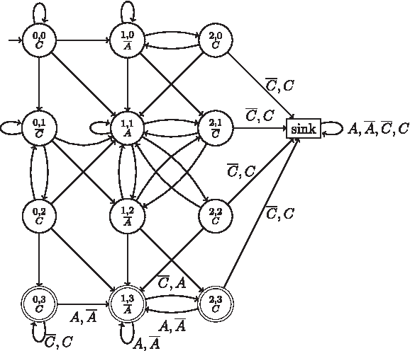
$${\cal N}^ \prime_b$$\end{document}. See an example of this automaton in Figure 2.
The automaton
\documentclass{aastex}
\usepackage{amsbsy}
\usepackage{amsfonts}
\usepackage{amssymb}
\usepackage{bm}
\usepackage{mathrsfs}
\usepackage{pifont}
\usepackage{stmaryrd}
\usepackage{textcomp}
\usepackage{portland, xspace}
\usepackage{amsmath, amsxtra}
\pagestyle{empty}
\DeclareMathSizes {10} {9} {7} {6}
\begin{document}
$${\cal N}^ \prime_{ACC}$$\end{document}. For the automaton to be readable, we use the notations
\documentclass{aastex}
\usepackage{amsbsy}
\usepackage{amsfonts}
\usepackage{amssymb}
\usepackage{bm}
\usepackage{mathrsfs}
\usepackage{pifont}
\usepackage{stmaryrd}
\usepackage{textcomp}
\usepackage{portland, xspace}
\usepackage{amsmath, amsxtra}
\pagestyle{empty}
\DeclareMathSizes {10} {9} {7} {6}
\begin{document}
$$A = {A \choose A} , {\overline{A}} = {A \choose C} , C = {C \choose C} ,$$\end{document} and
\documentclass{aastex}
\usepackage{amsbsy}
\usepackage{amsfonts}
\usepackage{amssymb}
\usepackage{bm}
\usepackage{mathrsfs}
\usepackage{pifont}
\usepackage{stmaryrd}
\usepackage{textcomp}
\usepackage{portland, xspace}
\usepackage{amsmath, amsxtra}
\pagestyle{empty}
\DeclareMathSizes {10} {9} {7} {6}
\begin{document}
$${\overline C} = {C \choose A}$$\end{document}. When the label of a transition is not given, it is by default set to the letter at the bottom of its ending state.
Lemma 3.2
Let u be a word in
\documentclass{aastex}
\usepackage{amsbsy}
\usepackage{amsfonts}
\usepackage{amssymb}
\usepackage{bm}
\usepackage{mathrsfs}
\usepackage{pifont}
\usepackage{stmaryrd}
\usepackage{textcomp}
\usepackage{portland, xspace}
\usepackage{amsmath, amsxtra}
\pagestyle{empty}
\DeclareMathSizes {10} {9} {7} {6}
\begin{document}
$${\cal B}^*$$\end{document}, and let qube the state reached after reading u in
\documentclass{aastex}
\usepackage{amsbsy}
\usepackage{amsfonts}
\usepackage{amssymb}
\usepackage{bm}
\usepackage{mathrsfs}
\usepackage{pifont}
\usepackage{stmaryrd}
\usepackage{textcomp}
\usepackage{portland, xspace}
\usepackage{amsmath, amsxtra}
\pagestyle{empty}
\DeclareMathSizes {10} {9} {7} {6}
\begin{document}
$${\cal N}_b^{\prime}$$\end{document}from its initial state. The words u can be classified as follows:
•
\documentclass{aastex}
\usepackage{amsbsy}
\usepackage{amsfonts}
\usepackage{amssymb}
\usepackage{bm}
\usepackage{mathrsfs}
\usepackage{pifont}
\usepackage{stmaryrd}
\usepackage{textcomp}
\usepackage{portland, xspace}
\usepackage{amsmath, amsxtra}
\pagestyle{empty}
\DeclareMathSizes {10} {9} {7} {6}
\begin{document}
$$q_u \in F^{\prime}$$\end{document}then π0(u) does not contains b but π1(u) does (this is a success in our settings);
• if qu is the sink state then π0(u) contains b (this is contradictory in our settings);
• if
\documentclass{aastex}
\usepackage{amsbsy}
\usepackage{amsfonts}
\usepackage{amssymb}
\usepackage{bm}
\usepackage{mathrsfs}
\usepackage{pifont}
\usepackage{stmaryrd}
\usepackage{textcomp}
\usepackage{portland, xspace}
\usepackage{amsmath, amsxtra}
\pagestyle{empty}
\DeclareMathSizes {10} {9} {7} {6}
\begin{document}
$$q_u \, \notin \, F^{\prime}$$\end{document} and qu is not the sink state, then neither π0(u) nor π1(u) contains b (this is a failure in our settings).
From automata to probabilities
The automaton
\documentclass{aastex}
\usepackage{amsbsy}
\usepackage{amsfonts}
\usepackage{amssymb}
\usepackage{bm}
\usepackage{mathrsfs}
\usepackage{pifont}
\usepackage{stmaryrd}
\usepackage{textcomp}
\usepackage{portland, xspace}
\usepackage{amsmath, amsxtra}
\pagestyle{empty}
\DeclareMathSizes {10} {9} {7} {6}
\begin{document}
$${\cal N}_b^{\prime}$$\end{document} is readily transformed into a Markov chain, by changing the label of any transition
\documentclass{aastex}
\usepackage{amsbsy}
\usepackage{amsfonts}
\usepackage{amssymb}
\usepackage{bm}
\usepackage{mathrsfs}
\usepackage{pifont}
\usepackage{stmaryrd}
\usepackage{textcomp}
\usepackage{portland, xspace}
\usepackage{amsmath, amsxtra}
\pagestyle{empty}
\DeclareMathSizes {10} {9} {7} {6}
\begin{document}
$$q \mathop{\rightarrow} \limits^{a} q^{\prime}$$\end{document}, where
\documentclass{aastex}
\usepackage{amsbsy}
\usepackage{amsfonts}
\usepackage{amssymb}
\usepackage{bm}
\usepackage{mathrsfs}
\usepackage{pifont}
\usepackage{stmaryrd}
\usepackage{textcomp}
\usepackage{portland, xspace}
\usepackage{amsmath, amsxtra}
\pagestyle{empty}
\DeclareMathSizes {10} {9} {7} {6}
\begin{document}
$$a = {\alpha \choose \beta} \in {\cal B}$$\end{document}, into the probability ν(α) × pα,β(1). If there are several transitions from q to q′, the edge is labelled by the sum of the associated probabilities. Let
\documentclass{aastex}
\usepackage{amsbsy}
\usepackage{amsfonts}
\usepackage{amssymb}
\usepackage{bm}
\usepackage{mathrsfs}
\usepackage{pifont}
\usepackage{stmaryrd}
\usepackage{textcomp}
\usepackage{portland, xspace}
\usepackage{amsmath, amsxtra}
\pagestyle{empty}
\DeclareMathSizes {10} {9} {7} {6}
\begin{document}
$${\cal C}_b$$\end{document} denote this Markov chain. The random variable Qn associated to the state reached after reading a random word of size n under the M0 model is formally defined by:
\documentclass{aastex}
\usepackage{amsbsy}
\usepackage{amsfonts}
\usepackage{amssymb}
\usepackage{bm}
\usepackage{mathrsfs}
\usepackage{pifont}
\usepackage{stmaryrd}
\usepackage{textcomp}
\usepackage{portland, xspace}
\usepackage{amsmath, amsxtra}
\pagestyle{empty}
\DeclareMathSizes {10} {9} {7} {6}
\begin{document}
\begin{align*}\forall q \in Q^{\prime} , \ \Pr ( Q_n = q ) = \sum_{\textstyle{u = {v \choose w} \in {\cal B}^n \atop \delta^{\prime} ( q^{\prime}_0 , u ) = q}} \nu ( v ) \times p_{v \rightarrow w} ( 1 ) . \tag{5}\end{align*}\end{document}
Then, if
\documentclass{aastex}
\usepackage{amsbsy}
\usepackage{amsfonts}
\usepackage{amssymb}
\usepackage{bm}
\usepackage{mathrsfs}
\usepackage{pifont}
\usepackage{stmaryrd}
\usepackage{textcomp}
\usepackage{portland, xspace}
\usepackage{amsmath, amsxtra}
\pagestyle{empty}
\DeclareMathSizes {10} {9} {7} {6}
\begin{document}
$${\mathbb P}_b$$\end{document} is the transition matrix of
\documentclass{aastex}
\usepackage{amsbsy}
\usepackage{amsfonts}
\usepackage{amssymb}
\usepackage{bm}
\usepackage{mathrsfs}
\usepackage{pifont}
\usepackage{stmaryrd}
\usepackage{textcomp}
\usepackage{portland, xspace}
\usepackage{amsmath, amsxtra}
\pagestyle{empty}
\DeclareMathSizes {10} {9} {7} {6}
\begin{document}
$${\cal C}_b$$\end{document} and if Vq is the probability vector with 1 on position
\documentclass{aastex}
\usepackage{amsbsy}
\usepackage{amsfonts}
\usepackage{amssymb}
\usepackage{bm}
\usepackage{mathrsfs}
\usepackage{pifont}
\usepackage{stmaryrd}
\usepackage{textcomp}
\usepackage{portland, xspace}
\usepackage{amsmath, amsxtra}
\pagestyle{empty}
\DeclareMathSizes {10} {9} {7} {6}
\begin{document}
$$q \in Q^{\prime}$$\end{document} and 0 elsewhere, the random state Qn reached from the initial state after n steps verifies
\documentclass{aastex}
\usepackage{amsbsy}
\usepackage{amsfonts}
\usepackage{amssymb}
\usepackage{bm}
\usepackage{mathrsfs}
\usepackage{pifont}
\usepackage{stmaryrd}
\usepackage{textcomp}
\usepackage{portland, xspace}
\usepackage{amsmath, amsxtra}
\pagestyle{empty}
\DeclareMathSizes {10} {9} {7} {6}
\begin{document}
\begin{align*}\forall q \in Q^{\prime} , \ \Pr ( Q_n = q ) = V_{q^{\prime}_0}^t \times {\mathbb P}_b^n \times V_{q}. \tag{6}\end{align*}\end{document}
Applying Equation (10) for obtaining the automaton results and using Theorem 1 from Behrens and Vingron (2010), we computed the expected waiting time E(T1000) of all k-mers in the M0 model for k from 5 to 10 to appear in a promoter sequence of length 1000 bp. The parameters of model M0 have been estimated as described in Section 2 and are depicted in Table 1.
Figure 3 provides an overall comparison of the waiting time computed by automata with respect to the previous computations of Behrens and Vingron (2010) for k = 5 and k = 10. As can be observed in this scatterplot, the computed waiting times based on the automaton approach globally confirm the results of Behrens and Vingron (2010). However, there are some outliers exhibiting longer waiting times than predicted by Behrens and Vingron (2010). The four most extreme outliers that deviate from the bisecting line correspond to AAAAA, TTTTT, CCCCC, and GGGGG, and to AAAAAAAAAA, CCCCCCCCCC, GGGGGGGGGG, and TTTTTTTTTT, respectively. Other outliers are k-mers like e.g. CGCGC, TCTCT and CGCGCGCGCG, TCTCTCTCTC. Tables 2–4 show all 5−, 7−, and 10-mers for which
\documentclass{aastex}
\usepackage{amsbsy}
\usepackage{amsfonts}
\usepackage{amssymb}
\usepackage{bm}
\usepackage{mathrsfs}
\usepackage{pifont}
\usepackage{stmaryrd}
\usepackage{textcomp}
\usepackage{portland, xspace}
\usepackage{amsmath, amsxtra}
\pagestyle{empty}
\DeclareMathSizes {10} {9} {7} {6}
\begin{document}
$$ \frac {{\bf E} _ {\rm BNN} \, ( T_ {1000} )} {{\bf E} _ {\rm BV} \, ( T_ {1000} )} $$\end{document} > 1.05 where EBV(T1000) denotes the expected waiting time according to Behrens and Vingron (2010) and EBNN(T1000) according to our automaton approach, i.e. k-mers with significantly longer waiting times than predicted by Behrens and Vingron (2010).
Overall comparisons of waiting times of Behrens and Vingron (2010) (BV) versus the automata method (BNN) for 5- and 10-mers.
EBV(T1000) denotes the expected waiting time according to Behrens and Vingron (2010) (BV) and EBNN(T1000) according to our automaton approach (BNN). Ranks refer to 5-mers sorted by their waiting time of appearance according to the two different procedures BV and BNN; rank 1 is assigned to the fastest evolving 5-mer, rank 1024 ( = 45) to the slowest emerging 5-mer.
EBV(T1000) denotes the expected waiting time according to Behrens and Vingron (2010) (BV) and EBNN(T1000) according to our automaton approach (BNN). Ranks refer to 7-mers sorted by their waiting time of appearance according to the two different procedures BV and BNN; rank 1 is assigned to the fastest evolving 7-mer, rank 16384 ( = 47) to the slowest emerging 7-mer.
EBV(T1000) denotes the expected waiting time according to Behrens and Vingron (2010) (BV) and EBNN(T1000) according to our automaton approach (BNN). Ranks refer to 10-mers sorted by their waiting time of appearance according to the two different procedures BV and BNN; rank 1 is assigned to the fastest evolving 10-mer, rank 1048576 ( = 410) to the slowest emerging 10-mer.
We use in the following the million of generations (in short Mgen) as unit of time, where a generation is 20 years. The discrepancy between the two procedures can attain up to around 40%, e.g., CCCCC has a discrepancy of 44% with EBNN(T1000) = 9.105 Mgen and EBV(T1000) = 6.304 Mgen, CCCCCCC a discrepancy of 43% with EBNN(T1000) = 93.457 Mgen and EBV(T1000) = 65.518 Mgen, and CCCCCCCCCC has a discrepancy of 41% with EBNN(T1000) = 3577.003 Mgen and EBV(T1000) = 2545.561 Mgen. Strikingly, most of the k-mers with significant discrepancy feature a high autocorrelation (i.e., they can appear overlapping in so-called clumps). For example, the 5-mer CCCCC could appear twice in the clump CCCCCC (at positions 1 and 2), CGCGC could appear three times in the clump CGCGCGCGC (at positions 1, 3, and 5). In order to distinguish between different levels of autocorrelation of k-mers, let
\documentclass{aastex}
\usepackage{amsbsy}
\usepackage{amsfonts}
\usepackage{amssymb}
\usepackage{bm}
\usepackage{mathrsfs}
\usepackage{pifont}
\usepackage{stmaryrd}
\usepackage{textcomp}
\usepackage{portland, xspace}
\usepackage{amsmath, amsxtra}
\pagestyle{empty}
\DeclareMathSizes {10} {9} {7} {6}
\begin{document}
\begin{align*}{\cal P} ( b ) : = \{p \in \{1 , \ldots , k - 1 \} :b_i = b_{i + p} \ {\rm for \ all} \ i = 1 , \ldots , k - p \} \end{align*}\end{document}
denote the set of periods of a k-mer
\documentclass{aastex}
\usepackage{amsbsy}
\usepackage{amsfonts}
\usepackage{amssymb}
\usepackage{bm}
\usepackage{mathrsfs}
\usepackage{pifont}
\usepackage{stmaryrd}
\usepackage{textcomp}
\usepackage{portland, xspace}
\usepackage{amsmath, amsxtra}
\pagestyle{empty}
\DeclareMathSizes {10} {9} {7} {6}
\begin{document}
$$b = ( b_1 , \ldots , b_k )$$\end{document}. A k-mer b is called non-periodic or non-autocorrelated if and only if
\documentclass{aastex}
\usepackage{amsbsy}
\usepackage{amsfonts}
\usepackage{amssymb}
\usepackage{bm}
\usepackage{mathrsfs}
\usepackage{pifont}
\usepackage{stmaryrd}
\usepackage{textcomp}
\usepackage{portland, xspace}
\usepackage{amsmath, amsxtra}
\pagestyle{empty}
\DeclareMathSizes {10} {9} {7} {6}
\begin{document}
$${\cal P} ( b ) = \emptyset$$\end{document}. Furthermore, for a periodic k-mer b let p0(b) denote its minimal period. For example, p0(CCCCC) = 1, p0(CGCGC) = 2, p0(CGACG) = 3, and p0(CGATC) = 4. We then call a word p-periodic if and only if its minimal period is p. As can be observed in Tables 2–4, half of the 5-mers, two-thirds of the 7-mers, and all of the 10-mers with
\documentclass{aastex}
\usepackage{amsbsy}
\usepackage{amsfonts}
\usepackage{amssymb}
\usepackage{bm}
\usepackage{mathrsfs}
\usepackage{pifont}
\usepackage{stmaryrd}
\usepackage{textcomp}
\usepackage{portland, xspace}
\usepackage{amsmath, amsxtra}
\pagestyle{empty}
\DeclareMathSizes {10} {9} {7} {6}
\begin{document}
$$ \frac {{\bf E} _ {\rm BNN} ( T_ {1000} )} {{\bf E} _ {\rm BV} ( T_ {1000} )} $$\end{document} > 1.05 are either 1- or 2-periodic (i.e., show a high degree of autocorrelation).
Behrens and Vingron (2010) already investigated the speed of TF binding site emergence and its biological implications for the evolution of transcriptional regulation in detail and we do not want to elaborate on this again. However, in line with Behrens and Vingron (2010), we want to emphasize that the speed of TF binding site emergence is primarily influenced by its nucleotide composition. The goal in the following will be to investigate the impact of autocorrelation regarding TF binding sites. More precisely, we want to answer the question: Do existing TF binding sites show significant autocorrelation or can this aspect be neglected when studying the speed of TF binding site emergence?
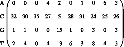
To investigate this, starting from the JASPAR CORE database for vertebrates Version 4 (Portales-Casamar et al., 2010), we extracted all the human TF binding sites of length k, 5 ≤ k ≤ 10, ending up with a set of 37 position count matrices (PCMs) for the 37 different TFs in analogy to Behrens and Vingron (2010). In order to make these PCMS accessible for our framework based on k-mers, we converted a PCM into a set of k-mers by setting a threshold of 0.95 of the maximal PCM score and extracted all k-mers with a score above this threshold. For example, the PCM
of the TF SP1 is then translated into the following set of 10-mers: {CCCCACCCCC, CCCCCCCCCC, CCCCGCCCCC, CCCCTCCCCC}. Applying this procedure, in total we obtain 372 different JASPAR k-mers, 5 ≤ k ≤ 10, for the 37 different human TFs. We then screened all JASPAR k-mers for 1-periodicity, 2-periodicity
\documentclass{aastex}
\usepackage{amsbsy}
\usepackage{amsfonts}
\usepackage{amssymb}
\usepackage{bm}
\usepackage{mathrsfs}
\usepackage{pifont}
\usepackage{stmaryrd}
\usepackage{textcomp}
\usepackage{portland, xspace}
\usepackage{amsmath, amsxtra}
\pagestyle{empty}
\DeclareMathSizes {10} {9} {7} {6}
\begin{document}
$$, \ldots ,$$\end{document} (k − 1)-periodicity. To evaluate the degree of autocorrelation of a given JASPAR TF given by its set of k-mers, we then computed the proportion of 1-periodic, 2-periodic
\documentclass{aastex}
\usepackage{amsbsy}
\usepackage{amsfonts}
\usepackage{amssymb}
\usepackage{bm}
\usepackage{mathrsfs}
\usepackage{pifont}
\usepackage{stmaryrd}
\usepackage{textcomp}
\usepackage{portland, xspace}
\usepackage{amsmath, amsxtra}
\pagestyle{empty}
\DeclareMathSizes {10} {9} {7} {6}
\begin{document}
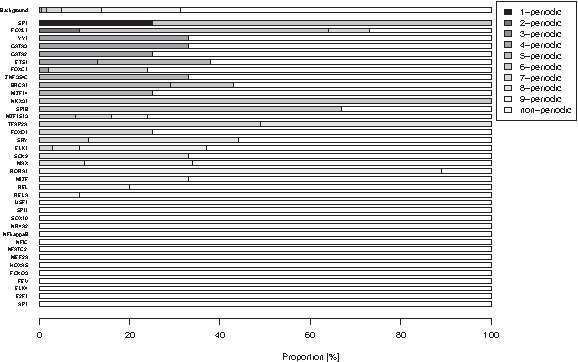
$$, \ldots ,$$\end{document} (k − 1)-periodic and of non-periodic k-mers in this set. The results are depicted in Figure 4. As can be seen, some TFs like SP1, FOXL1, YY1, GATA3, GATA2, and ETS1 exhibit a high autocorrelation, while 14 of the 37 TFs show no autocorrelation at all (USF1, SPI1,
\documentclass{aastex}
\usepackage{amsbsy}
\usepackage{amsfonts}
\usepackage{amssymb}
\usepackage{bm}
\usepackage{mathrsfs}
\usepackage{pifont}
\usepackage{stmaryrd}
\usepackage{textcomp}
\usepackage{portland, xspace}
\usepackage{amsmath, amsxtra}
\pagestyle{empty}
\DeclareMathSizes {10} {9} {7} {6}
\begin{document}
$$, \ldots ,$$\end{document} AP1). In order to test whether autocorrelated k-mers are enriched among JASPAR TF binding sites, as a background we screened all possible k-mers, i.e., all
\documentclass{aastex}
\usepackage{amsbsy}
\usepackage{amsfonts}
\usepackage{amssymb}
\usepackage{bm}
\usepackage{mathrsfs}
\usepackage{pifont}
\usepackage{stmaryrd}
\usepackage{textcomp}
\usepackage{portland, xspace}
\usepackage{amsmath, amsxtra}
\pagestyle{empty}
\DeclareMathSizes {10} {9} {7} {6}
\begin{document}
$$b = ( b_1 , \ldots , b_k ) \in{\cal A}^k , {\cal A} = {\{ \rm A , C , G , T \}}$$\end{document}, k ranging from 5 to 10, for autocorrelation in the same way as JASPAR k-mers. The resulting proportions of periodic and non-periodic words of this background are also depicted in Figure 4. In total, among the JASPAR k-mers, there are 168 autocorrelated words (i.e., words that are p-periodic for one
\documentclass{aastex}
\usepackage{amsbsy}
\usepackage{amsfonts}
\usepackage{amssymb}
\usepackage{bm}
\usepackage{mathrsfs}
\usepackage{pifont}
\usepackage{stmaryrd}
\usepackage{textcomp}
\usepackage{portland, xspace}
\usepackage{amsmath, amsxtra}
\pagestyle{empty}
\DeclareMathSizes {10} {9} {7} {6}
\begin{document}
$$p \in \{1\, . \, . \, k - 1 \} $$\end{document}) and 204 non-autocorrelated words. The background set contains 435,828 autocorrelated and 961,932 non-autocorrelated k-mers. Performing Fisher's Exact Test for Count Data with the alternative “greater,” we obtain a p-value of 1.119e-08. We can thus conclude that autocorrelated words are significantly enriched among JASPAR k-mers. Consequently, existing TF binding sites indeed feature a significant proportion of autocorrelation.
Barplot of the degree of autocorrelation of JASPAR TF binding sites. For every of the 37 JASPAR TFs each given by a set of k-mers, the proportion of p-periodic and non-periodic k-mers in this set was calculated, p ranging from 1 to k − 1. Additionally, the same proportions were computed for all possible k-mers, k ranging from 5 to 10 (“Background”).
In Section 3, we considered by automata a parallel computation on two sequences, S(0) and S(1).
It is possible to do a relevant mathematical analysis with the random sequence S(0) only. The corresponding computations have however a much higher complexity than the automaton approach. This analysis is defined on counting in a random sequence S(0) the number of putative-hit positions where, given a k-mer b, a putative-hit position is any position of S(0) that can lead by mutation to an occurrence of b in S(1), assuming that a single mutation has occurred.
For any k-mer b, Nicodème (2011) provides a combinatorial construction using clumps (see Bassino et al., 2008) that (i) considers all the sequences that avoid the k-mer b, and (ii) counts all the putative-hit position in these sequences.
In the following, let Hn denote the number of putative-hit positions in a sequence S(0) randomly chosen within the set of sequences of length n that do not contain the k-mer b, where the letters are drawn with respect to the distribution ν and where we put a probability mass 1 to the set.1 As a consequence of singularity analysis of rational functions, Nicodème (2011) proves that
\documentclass{aastex}
\usepackage{amsbsy}
\usepackage{amsfonts}
\usepackage{amssymb}
\usepackage{bm}
\usepackage{mathrsfs}
\usepackage{pifont}
\usepackage{stmaryrd}
\usepackage{textcomp}
\usepackage{portland, xspace}
\usepackage{amsmath, amsxtra}
\pagestyle{empty}
\DeclareMathSizes {10} {9} {7} {6}
\begin{document}
\begin{align*}{\bf E} ( H_n ) = c_1 \times \ n + c_2 + O ( A^n ) \qquad ( A < 1 ) . \tag{11}\end{align*}\end{document}
It is clear that, using the asymptotic Landau's Θ notation, we do not have
\documentclass{aastex}
\usepackage{amsbsy}
\usepackage{amsfonts}
\usepackage{amssymb}
\usepackage{bm}
\usepackage{mathrsfs}
\usepackage{pifont}
\usepackage{stmaryrd}
\usepackage{textcomp}
\usepackage{portland, xspace}
\usepackage{amsmath, amsxtra}
\pagestyle{empty}
\DeclareMathSizes {10} {9} {7} {6}
\begin{document}
\begin{align*}p_n = \Theta ( {\bf E} ( H_n ) ) ,\end{align*}\end{document}
the probability that two or more putative-hit positions simultaneously mutate to provide the k-mer b in sequence S(1) is an event of second order small probability. With these conditions, we have
\documentclass{aastex}
\usepackage{amsbsy}
\usepackage{amsfonts}
\usepackage{amssymb}
\usepackage{bm}
\usepackage{mathrsfs}
\usepackage{pifont}
\usepackage{stmaryrd}
\usepackage{textcomp}
\usepackage{portland, xspace}
\usepackage{amsmath, amsxtra}
\pagestyle{empty}
\DeclareMathSizes {10} {9} {7} {6}
\begin{document}
\begin{align*}p_n \approx \rho_{b , \nu , p} \times {\bf E} ( H_n ) = \rho_{b , \nu , p} \times ( c_1 \times n + c_2 ) + O ( A^n ) , \tag{12}\end{align*}\end{document}
where ρb,ν,p is a constant of the order of magnitude of the constants pα,β(1) with α ≠ β, its value depending upon these constants, the distribution ν and the correlation structure of the k-mer b. (Fig. 5).
Plots of the probability
\documentclass{aastex}
\usepackage{amsbsy}
\usepackage{amsfonts}
\usepackage{amssymb}
\usepackage{bm}
\usepackage{mathrsfs}
\usepackage{pifont}
\usepackage{stmaryrd}
\usepackage{textcomp}
\usepackage{portland, xspace}
\usepackage{amsmath, amsxtra}
\pagestyle{empty}
\DeclareMathSizes {10} {9} {7} {6}
\begin{document}
$$p_n$$\end{document}(left) and of the expected waiting time E(Tn) (right). (Top)b = AAAAA (blue) and b′ = CGCGC (magenta). (Bottom) b = CCCCCCCCCC (blue) and b′ = ATATATATAT (magenta). In the linear plots of the probability, the anchors values for n = 1000 and n = 2000 (computed by automata) are represented by boxes; the straight lines are the straight lines going through the corresponding points and the circles are test values also computed by automata. The fit is perfect as expected from singularity analysis.
Available data. URL www.lipn.univ-paris13.fr/∼nicodeme/ provides access to the values of the expected waiting time E(Tn) and the probability
\documentclass{aastex}
\usepackage{amsbsy}
\usepackage{amsfonts}
\usepackage{amssymb}
\usepackage{bm}
\usepackage{mathrsfs}
\usepackage{pifont}
\usepackage{stmaryrd}
\usepackage{textcomp}
\usepackage{portland, xspace}
\usepackage{amsmath, amsxtra}
\pagestyle{empty}
\DeclareMathSizes {10} {9} {7} {6}
\begin{document}
$$p_n$$\end{document} for n = 1000 and n = 2000 for all k-mers with k from 5 to 10. It is therefore possible to compute
\documentclass{aastex}
\usepackage{amsbsy}
\usepackage{amsfonts}
\usepackage{amssymb}
\usepackage{bm}
\usepackage{mathrsfs}
\usepackage{pifont}
\usepackage{stmaryrd}
\usepackage{textcomp}
\usepackage{portland, xspace}
\usepackage{amsmath, amsxtra}
\pagestyle{empty}
\DeclareMathSizes {10} {9} {7} {6}
\begin{document}
$$p_n$$\end{document} and E(Tn) for all these k-mers for all n from these data. It took 10 hours to compute the data.
6. Conclusion
Using automata theory, we have developed a new procedure to compute the waiting time until a given TF binding site emerges at random in a human promoter sequence. In contrast to Behrens and Vingron (2010), we do not have to rely on any assumptions regarding the overlap structure of the TF binding site of interest. Thus, our computations are more accurate. Assuming model M0, whose parameters have been estimated in the same way as in Behrens and Vingron (2010), applying our automaton approach to all k-mers, k ranging from 5 to 10, and comparing the resulting expected waiting times to those obtained by Behrens and Vingron (2010), we particularly observe that highly autocorrelated words like CCCCC actually tend to emerge slower than predicted by Behrens and Vingron (2010). This slowdown can attain up to 40%; for example, according to Behrens and Vingron (2010), CCCCC is predicted to be created in a human promoter of length 1 kb in around 6.304 Mgen, while our more accurate method predicts it be generated in around 9.105 Mgen. We have shown that existing TF binding sites (from the database JASPAR [Portales-Casamar et al., 2010]) feature a significant proportion of autocorrelation. Therefore, the assumption of Behrens and Vingron (2010) that TF binding sites do not appear self-overlapping when computing waiting times is problematic. The new automaton approach now incorporates the possibility of TF binding sites appearing self-overlapping into the model. Hence, the automaton approach highly improves the accuracy of the estimations for waiting times. We observed a linear behavior with respect to the length of the promoters for the probability of finding a k-mer at generation 1 that is not present at generation 0. This implies a highly flexible and efficient approach for computing this probability for any promoter length, and in particular for lengths of highest interest (i.e., between 300 and 3000 bp). This also induces a hyperbolic behavior for the waiting time.
Footnotes
Acknowledgments
We thank Martin Vingron who initiated the previous work of Behrens and Vingron (), of which the present article is a follow-up.
Disclosure Statement
No competing financial interests exist.
1
This is done by unconditioning with respect to the fact that b does not occur in S(0), i.e by dividing the resulting expressions by
\documentclass{aastex}
\usepackage{amsbsy}
\usepackage{amsfonts}
\usepackage{amssymb}
\usepackage{bm}
\usepackage{mathrsfs}
\usepackage{pifont}
\usepackage{stmaryrd}
\usepackage{textcomp}
\usepackage{portland, xspace}
\usepackage{amsmath, amsxtra}
\pagestyle{empty}
\DeclareMathSizes {10} {9} {7} {6}
\begin{document}
$$\Pr ( S ( 0 ) \not \in {\cal A}^*b{\cal A}^* )$$\end{document}; see .
References
1.
ArndtP.F., HwaT.2005. Identification and measurement of neighbor-dependent nucleotide substitution processes. Bioinformatics, 21:2322–2328.
2.
BassinoF., ClémentJ., FayolleJ.et al.2008. Constructions for clump statistics. Proc. 5th Colloq. Math. Comput. Sci., 183–198.
3.
BehrensS., VingronM.2010. Studying the evolution of promoters: a waiting time problem. J. Comput. Biol., 17:1591–1606.
4.
CrochemoreM., RytterW.1994. Text Algorithms. Oxford University Press: New York.
5.
DowellR.D.2010. Transcription factor binding variation in the evolution of gene regulation. Trends Genet., 26:468–475.
6.
DuretL., ArndtP.F.2008. The impact of recombination on nucleotide substitutions in the human genome. PLoS Genet, 4.
7.
DurrettR., SchmidtD.2007. Waiting for regulatory sequences to appear. Ann. Appl. Probab., 17:1–32.
8.
FlajoletP., SedgewickR.2009. Analytic Combinatorics. Cambridge University Press: New York.
9.
GouldenI., JacksonD.1983. Combinatorial Enumeration. John Wiley: New York.
10.
GuibasL., OdlyzkoA.1981a. Periods in strings. J. Combin. Theory A, 19–42.
11.
GuibasL., OdlyzkoA.1981b. Strings overlaps, pattern matching, and non-transitive games. J. Combin. Theory A, 108–203.
12.
HopcroftJ., MotwaniR., UllmanJ.2001. Introduction to Automata Theory, Languages and Computation. Addison-Wesley: New York.
13.
KarlinS., TaylorH.1975. A First Course in Stochastic Processes, 2nd. Academic Press: New York.
14.
KunarsoG., ChiaN.-Y., JeyakaniJ.et al.2010. Transposable elements have rewired the core regulatory network of human embryonic stem cells. Nat. Genet., 42:631–634.
15.
LothaireM.2005. Applied Combinatorics on Words. Cambridge University Press: New York.
OdomD.T., DowellR.D., JacobsenE.S.et al.2007. Tissue-specific transcriptional regulation has diverged significantly between human and mouse. Nat. Genet., 39:730–732.
18.
Portales-CasamarE., ThongjueaS., KwonA.T.et al.2010. JASPAR 2010: the greatly expanded open-access database of transcription factor binding profiles. Nucleic Acids Res., 38:D105–D110.
19.
SchmidtD., WilsonM.D., BallesterB.et al.2010. Five-vertebrate chip-seq reveals the evolutionary dynamics of transcription factor binding. Science, 328:1036–1040.
20.
StoneJ.R., WrayG.A.2001. Rapid evolution of cis-regulatory sequences via local point mutations. Mol. Biol. Evol., 18:1764–1770.
21.
WrayG.A., HahnM.W., AbouheifE.et al.2003. The evolution of transcriptional regulation in eukaryotes. Mol. Biol. Evol., 20:1377–1419.