LB3D: A Protein Three-Dimensional Substructure Search Program Based on the Lower Bound of a Root Mean Square Deviation Value

Abstract

Searching for protein structure-function relationships using three-dimensional (3D) structural coordinates represents a fundamental approach for determining the function of proteins with unknown functions. Since protein structure databases are rapidly growing in size, the development of a fast search method to find similar protein substructures by comparison of protein 3D structures is essential. In this article, we present a novel protein 3D structure search method to find all substructures with root mean square deviations (RMSDs) to the query structure that are lower than a given threshold value. Our new algorithm runs in O(m + N/m^0.5) time, after O(N log N) preprocessing, where N is the database size and m is the query length. The new method is 1.8–41.6 times faster than the practically best known O(N) algorithm, according to computational experiments using a huge database (i.e., >20,000,000 C-alpha coordinates).

1 Introduction

Fundamental approaches used to identify the function of a protein employ search engines that group “similar” proteins based on their three-dimensional (3D) structures and/or amino acid sequences. Such approaches aid in the identification of protein functions because a protein with an unknown function may be grouped with proteins (or a protein) with a known function based on sequence or structural similarity. Due to the speed, quality, and ease of use, sequence search methods such as the popular BLAST and PSI-BLAST programs use sequence databases to find proteins that have similar sequences (Altschul et al., 1997). However, there is also a relationship between structural conservation and protein function even when there is low sequence similarity (Betts et al., 2001). Accordingly, the rapidly increasing number of 3D protein structures deposited in the Protein Data Bank (PDB (Berman et al., 2000), http://www.pdb.org/) is facilitating the identification of proteins with similar functions based on structural similarities.

Many computational approaches have been developed for structural comparison, including FAST (Zhu and Weng, 2005), CE (Shindyalov and Bourne, 1998), DALI (Holm and Sander, 1993), MAMMOTH (Ortiz et al., 2002), TM-Align (Zhang and Skolnick, 2005), and PSIST (Gao and Zaki, 2005). The majority of these algorithms are generally based on two steps. The first step involves a local geometric comparison of small regions for identifying structurally similar regions and residue pairs using the C-alpha atoms between two proteins. These alignments obtained by structural comparisons between small fragments are known as aligned fragment pairs (AFPs). AFPs are identified by sliding a window, which has a fixed size, between protein structures. The second step is the structural alignment of the global folds using a particular algorithm, such as dynamic programming. For example, in the first step that defines the AFPs, FAST compares two five-residue segments according to the similarity function based on Euclidian distances between C-alpha atoms. CE and DALI use a C-alpha distance matrix of local structures (eight and six residues, respectively). MAMMOTH uses the unit vector of small substructures (eight residues) and the unit-vector root mean square (URMS) distance between all pairs of heptapeptides as a similarity function. TM-Align employs secondary structure elements and the TM-Score to obtain the initial alignment. PSIST uses a distance and a bond angle as a feature vector within each window (three residues) to describe local features.

The structural alignment problem of proteins with insertions or deletions is known as the NP-hard problem (Lathrop, 1994). There are various heuristic approaches to solve the NP-hard problem, but no exact solution. In this article, we focus on an easier, but essential problem: finding all substructures of a 3D structure from a protein database whose root mean square deviation (RMSD) (Kabsch, 1976) to the query structure are given a threshold and contain no insertions or deletions. There is a simple solution to this problem involving the comparison between the query structure with all structures within a database; however, this method costs O(Nm) time, where N is the database size and m is the query length (Diamond, 1998; Umeyama, 1991). The best known algorithm is a filtering based algorithm (Shibuya, 2010a) that uses a lower bound RMSD to eliminate unrelated structures before computing the final RMSD. Shibuya proved that the filtering based method runs in O(N) time in the average case, though the worst-case time complexity is still O(Nm), which is the same as the above Naive algorithm. Here, we propose a significantly faster algorithm in practice that uses new lower bounds and runs in O(m + N/m^0.5) time in the average case, after O(N log N) preprocessing. Note that the worst-case time complexity of our algorithm is still O(Nm), as in the case of the previous best-known algorithm. The O(N log N) preprocessing time is theoretically worse than the previously best algorithm, but it is the time complexity for very simple sorting, and the actual computing time for it can be dismissed. Note also that there has been proposed an algorithm with better expected time complexity, i.e., O(m + N/m^1-ɛ) (Shibuya, 2010b), where is ɛ is an arbitrary small constant, but the algorithm is not a practical algorithm but a theoretical one. It is apparently not effective for ordinary query sizes (which are at most around 1,000), and moreover it is a very complicated algorithm and is extremely difficult to implement. Thus, we do not compare our algorithm with the theoretical best algorithm.

1.1 Problem definition

In the case that we are given a 3D structure database P which consists of a large number of protein molecules (over 110,000) and a query structure Q, the problem is to find all the substructures from P whose RMSDs to Q are at most a given fixed threshold c, without considering insertions or deletions. The goal is to execute an exhaustive search faster than known algorithms. When we considered “similar substructures,” we used the RMSD, which was defined as the square root of the minimum value of the average squared distance between corresponding residues after optimal rotation and translation of one structure to another structure. The RMSD is the most commonly used measure to compare protein structures. Therefore, we used the RMSD as a threshold for finding a solution to the 3D structure problem.

2 Methods

2.1 Notation and definitions

In this article, to describe the protein 3D structure, 3D coordinates of each residue were approximated by the C-alpha coordinates. A chain molecule S is represented as S = (s₁, s₂, … , s_n), where s_i denotes the 3D coordinates of the i-th C-alpha atom and n denotes the number of amino acids of S. |S| means the length of S. A structure S[i.j] = (s_i, s_i+1, … , s_j) is called a substructure of S from the i-th residue to the j-th residue. |S[i.j]| is equal to j−i + 1. \documentclass{aastex}\usepackage{amsbsy}\usepackage{amsfonts}\usepackage{amssymb}\usepackage{bm}\usepackage{mathrsfs}\usepackage{pifont}\usepackage{stmaryrd}\usepackage{textcomp}\usepackage{portland, xspace}\usepackage{amsmath, amsxtra}\pagestyle{empty}\DeclareMathSizes{10}{9}{7}{6}\begin{document} $$R \cdot S$$ \end{document} denotes the structure S rotated by the rotation matrix R. For two structures S = (s₁, s₂, … , s_n) and T = (t₁, t₂, … , t_n), the concatenated structure (s₁, s₂, … , s_n, t₁, t₂, … , t_n) is denoted by S + T. \documentclass{aastex}\usepackage{amsbsy}\usepackage{amsfonts}\usepackage{amssymb}\usepackage{bm}\usepackage{mathrsfs}\usepackage{pifont}\usepackage{stmaryrd}\usepackage{textcomp}\usepackage{portland, xspace}\usepackage{amsmath, amsxtra}\pagestyle{empty}\DeclareMathSizes{10}{9}{7}{6}\begin{document} $$\langle x \rangle$$ \end{document} denotes the expected value of x, var(x) denotes the variance of x and Pr(X) denotes the probability of event X.

2.2 Shibuya's lower bound for the RMSD

The RMSD between two chain molecules S and T is defined as the minimum value of \documentclass{aastex}\usepackage{amsbsy}\usepackage{amsfonts}\usepackage{amssymb}\usepackage{bm}\usepackage{mathrsfs}\usepackage{pifont}\usepackage{stmaryrd}\usepackage{textcomp}\usepackage{portland, xspace}\usepackage{amsmath, amsxtra}\pagestyle{empty}\DeclareMathSizes{10}{9}{7}{6}\begin{document} \begin{align*} \sqrt {\frac {1} {n} \sum_{i = 1}^n \Big| s_i - (R \cdot t_i + v) \Big|^2} \tag {1} \end{align*} \end{document}

over all the possible rotation matrices R and translation vectors v. RMSD(S, T) denotes this minimum value.

Shibuya proposed a lower bound for the RMSD between any two structures with the same length. When the chain molecule \documentclass{aastex}\usepackage{amsbsy}\usepackage{amsfonts}\usepackage{amssymb}\usepackage{bm}\usepackage{mathrsfs}\usepackage{pifont}\usepackage{stmaryrd}\usepackage{textcomp}\usepackage{portland, xspace}\usepackage{amsmath, amsxtra}\pagestyle{empty}\DeclareMathSizes{10}{9}{7}{6}\begin{document} $$U = (u_{\it 1}, \ u_{\it 2}, \ldots , \, u_n), \ U^{left}$$ \end{document} denotes \documentclass{aastex}\usepackage{amsbsy}\usepackage{amsfonts}\usepackage{amssymb}\usepackage{bm}\usepackage{mathrsfs}\usepackage{pifont}\usepackage{stmaryrd}\usepackage{textcomp}\usepackage{portland, xspace}\usepackage{amsmath, amsxtra}\pagestyle{empty}\DeclareMathSizes{10}{9}{7}{6}\begin{document} $$(u_1, \ u_2, \ldots, \, u_{\lfloor m/2 \rfloor})$$ \end{document} and U^right denotes \documentclass{aastex}\usepackage{amsbsy}\usepackage{amsfonts}\usepackage{amssymb}\usepackage{bm}\usepackage{mathrsfs}\usepackage{pifont}\usepackage{stmaryrd}\usepackage{textcomp}\usepackage{portland, xspace}\usepackage{amsmath, amsxtra}\pagestyle{empty}\DeclareMathSizes{10}{9}{7}{6}\begin{document} $$(u_{\lfloor m/2 \rfloor + 1}, \, u_{\lfloor m/2 + 2 \rfloor}, \ldots , \, u_{2\lfloor m/2 \rfloor})$$ \end{document} . G(U) denotes \documentclass{aastex}\usepackage{amsbsy}\usepackage{amsfonts}\usepackage{amssymb}\usepackage{bm}\usepackage{mathrsfs}\usepackage{pifont}\usepackage{stmaryrd}\usepackage{textcomp}\usepackage{portland, xspace}\usepackage{amsmath, amsxtra}\pagestyle{empty}\DeclareMathSizes{10}{9}{7}{6}\begin{document} $$\frac {1} {m} \sum\nolimits_{i = 1}^m u_i$$ \end{document} as the centroid of the structure U. Let F(U) denote |G(U^left) − G(U^right)|/2 and let D(S, T) denote \documentclass{aastex}\usepackage{amsbsy}\usepackage{amsfonts}\usepackage{amssymb}\usepackage{bm}\usepackage{mathrsfs}\usepackage{pifont}\usepackage{stmaryrd}\usepackage{textcomp}\usepackage{portland, xspace}\usepackage{amsmath, amsxtra}\pagestyle{empty}\DeclareMathSizes{10}{9}{7}{6}\begin{document} $$\sqrt{2 \cdot \mid S^{left} \mid / \mid S \mid} \cdot \mid F (S) - F (T) \mid$$ \end{document} for chain molecules S and T such that |S| = |T|. Shibuya proved that D(S, T) is smaller than or equal to RMSD(S, T).

The algorithm for searching for similar substructures with Shibuya's lower bound for the RMSD is simply described by two steps: (1) searching through all the substructures where the lower bound (D(S,T)) for a RMSD is lower than the given threshold c, and is therefore a candidate; and (2) the RMSD values of each candidate are then checked using the C-alpha coordinates. Even though the D(S,T) is not representative of the RMSD, it can be used as a filter to remove dissimilar substructures in simple calculations, because of the inequality such that D(S,T) is smaller than or equal to RMSD(S,T). If the D(S,T) is larger than the given threshold c, RMSD(S,T) must be larger than c.

Shibuya also proposed that the following lower bound for the RMSD using the combination of three segments is very efficient in removing dissimilar substructures before computing the actual RMSD. \documentclass{aastex}\usepackage{amsbsy}\usepackage{amsfonts}\usepackage{amssymb}\usepackage{bm}\usepackage{mathrsfs}\usepackage{pifont}\usepackage{stmaryrd}\usepackage{textcomp}\usepackage{portland, xspace}\usepackage{amsmath, amsxtra}\pagestyle{empty}\DeclareMathSizes{10}{9}{7}{6}\begin{document} \begin{align*} RMSD (P [ i..i + m - 1 ] , Q) \geq \sqrt {\frac {m^{\prime}} {m}} \cdot \left\{\sum_{j = 1}^3 (RMSD (P [ i + (j - 1) \cdot m^{\prime} ..i + j \cdot m^{\prime} - 1 ] , Q [ 1 + (j - 1) \cdot m^{\prime} ..j \cdot m^{\prime} ]))^2 \right\}^{1 / 2} \tag {2} \end{align*} \end{document} \documentclass{aastex}\usepackage{amsbsy}\usepackage{amsfonts}\usepackage{amssymb}\usepackage{bm}\usepackage{mathrsfs}\usepackage{pifont}\usepackage{stmaryrd}\usepackage{textcomp}\usepackage{portland, xspace}\usepackage{amsmath, amsxtra}\pagestyle{empty}\DeclareMathSizes{10}{9}{7}{6}\begin{document} \begin{align*} \geq \sqrt {\frac {m^{\prime}} {m}} \cdot \left\{\sum_{j = 1}^3 (D (P [ i + (j - 1) \cdot m^{\prime} ..i + j \cdot m^{\prime} - 1 ] , Q [ 1 + (j - 1) \cdot m^{\prime} ..j \cdot m^{\prime} ]))^2 \right\}^{1 / 2} \tag {3} \end{align*} \end{document}

where \documentclass{aastex}\usepackage{amsbsy}\usepackage{amsfonts}\usepackage{amssymb}\usepackage{bm}\usepackage{mathrsfs}\usepackage{pifont}\usepackage{stmaryrd}\usepackage{textcomp}\usepackage{portland, xspace}\usepackage{amsmath, amsxtra}\pagestyle{empty}\DeclareMathSizes{10}{9}{7}{6}\begin{document} $$m^{\prime} = \lfloor m / 3 \rfloor$$ \end{document} , and P and Q denote the protein structure database and query structure, respectively.

Shibuya reported that the algorithm (denoted as A3: Algorithm 3) with this lower bound (expression (3)) for the RMSD is much faster than other algorithms.

2.3 New lower bounds for the RMSD

Now we consider P[i.i + m−1] and Q as a chain molecule consisting of six segments which have the same length \documentclass{aastex}\usepackage{amsbsy}\usepackage{amsfonts}\usepackage{amssymb}\usepackage{bm}\usepackage{mathrsfs}\usepackage{pifont}\usepackage{stmaryrd}\usepackage{textcomp}\usepackage{portland, xspace}\usepackage{amsmath, amsxtra}\pagestyle{empty}\DeclareMathSizes{10}{9}{7}{6}\begin{document} $$m^{\prime \prime}$$ \end{document} . Let \documentclass{aastex}\usepackage{amsbsy}\usepackage{amsfonts}\usepackage{amssymb}\usepackage{bm}\usepackage{mathrsfs}\usepackage{pifont}\usepackage{stmaryrd}\usepackage{textcomp}\usepackage{portland, xspace}\usepackage{amsmath, amsxtra}\pagestyle{empty}\DeclareMathSizes{10}{9}{7}{6}\begin{document} $$m^{\prime \prime} = \lfloor m^{\prime} / 2 \rfloor , P_{i , j} = P [ i + (j - 1) \cdot m^{\prime \prime} . .i + j \cdot m^{\prime \prime} - 1 ]$$ \end{document} , and \documentclass{aastex}\usepackage{amsbsy}\usepackage{amsfonts}\usepackage{amssymb}\usepackage{bm}\usepackage{mathrsfs}\usepackage{pifont}\usepackage{stmaryrd}\usepackage{textcomp}\usepackage{portland, xspace}\usepackage{amsmath, amsxtra}\pagestyle{empty}\DeclareMathSizes{10}{9}{7}{6}\begin{document} $$Q_j = Q [ 1 + (j - 1) \cdot m^{\prime \prime} . . j \cdot m^{\prime \prime} ]$$ \end{document} . P_i,j represents the j-th segment among the six for position i in the database P. Q_j represents the j-th among the six segments of the query Q (Fig. 1A). The lower bound for the RMSD is described as follows: \documentclass{aastex}\usepackage{amsbsy}\usepackage{amsfonts}\usepackage{amssymb}\usepackage{bm}\usepackage{mathrsfs}\usepackage{pifont}\usepackage{stmaryrd}\usepackage{textcomp}\usepackage{portland, xspace}\usepackage{amsmath, amsxtra}\pagestyle{empty}\DeclareMathSizes{10}{9}{7}{6}\begin{document} \begin{align*} & RMSD (P [ i..i + m - 1 ] , Q) \geq \sqrt {\frac {m^{\prime}} {m}} \cdot \left\{ \sum_{j = 1}^3 (RMSD (P [ i + (j - 1) \cdot 2m^{\prime \prime} ..i + j \cdot 2m^{\prime \prime} - 1 ] , \ Q [ 1 + (j - 1) \cdot 2m^{\prime \prime} ..j \cdot 2m^{\prime \prime} ]))^2 \right\} \\ &\geq \sqrt {\frac {m^{\prime}} {m}} \cdot \left\{\sum_{j = 1}^3 (RMSD (P [ i + (j - 1) \cdot 2m^{\prime \prime} ..i + (2j - 1) \cdot m^{\prime \prime} - 1 ] + P [ i + (2j - 1) \cdot m^{\prime \prime} ..i + j \cdot 2 m^{\prime \prime} - 1 ] , \ Q [ 1 + (j - 1) \cdot 2m^{\prime \prime} .. (2j - 1) \cdot m^{\prime \prime} ] + Q [ 1 + 2j - 1) \cdot m^{\prime \prime} ..j \cdot 2 m^{\prime \prime} ]))^2 \right\}^{1 / 2} \tag{4} \end{align*} \end{document} \documentclass{aastex}\usepackage{amsbsy}\usepackage{amsfonts}\usepackage{amssymb}\usepackage{bm}\usepackage{mathrsfs}\usepackage{pifont}\usepackage{stmaryrd}\usepackage{textcomp}\usepackage{portland, xspace}\usepackage{amsmath, amsxtra}\pagestyle{empty}\DeclareMathSizes{10}{9}{7}{6}\begin{document} \begin{align*} = \sqrt {\frac {m^{\prime}} {m}} \cdot \left\{RMSD \left(P_{i , 1} + P_{i , 2} , Q_1 + Q_2 \right)^2 + RMSD \left(P_{i , 3} + P_{i , 4} , Q_3 + Q_4 \right)^2 + RMSD \left(P_{i , 5} + P_{i , 6} , Q_5 + Q_6 \right)^2 \right\}^{1 / 2} \tag {5} \end{align*} \end{document} \documentclass{aastex}\usepackage{amsbsy}\usepackage{amsfonts}\usepackage{amssymb}\usepackage{bm}\usepackage{mathrsfs}\usepackage{pifont}\usepackage{stmaryrd}\usepackage{textcomp}\usepackage{portland, xspace}\usepackage{amsmath, amsxtra}\pagestyle{empty}\DeclareMathSizes{10}{9}{7}{6}\begin{document} \begin{align*} \geq \sqrt {\frac {m^{\prime}} {m}} \cdot \left\{D (P_{i , 1} + P_{i , 2} , Q_1 + Q_2)^2 + D (P_{i , 3} + P_{i , 4} , Q_3 + Q_4)^2 + D (P_{i , 5} + P_{i , 6} , Q_5 + Q_6)^2 \right\}^{1 / 2} \tag {6} \end{align*} \end{document}

Fig. 1.

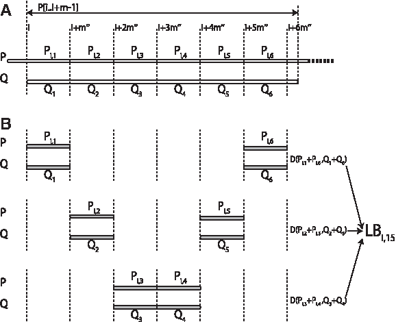
A: Illustration of the six segments for position i in database (P_i,1 − P_i,6) and query (Q₁ − Q₆). B: Example of LB_i,15 (expression(23)). LB_i,15 consists three lower bounds of combined segments (D(P_i,1 + P_i,6, Q₁ + Q₆), (D(P_i,2 + P_i,5, Q₂ + Q₅) and (D(P_i,3 + P_i,4, Q₃ + Q₄)).

The expression (6) shows that the lower bound can be described as a comparison between two chain molecules consisting of six segments (P_i,1 − P_i,6 and Q₁ − Q₆). We then consider the combination of two segments among the six segments as: \documentclass{aastex}\usepackage{amsbsy}\usepackage{amsfonts}\usepackage{amssymb}\usepackage{bm}\usepackage{mathrsfs}\usepackage{pifont}\usepackage{stmaryrd}\usepackage{textcomp}\usepackage{portland, xspace}\usepackage{amsmath, amsxtra}\pagestyle{empty}\DeclareMathSizes{10}{9}{7}{6}\begin{document} \begin{align*} LB_i (a , b , c , d , e , f) = \sqrt {\frac {m^{\prime}} {m}} \cdot \left\{D (P_{i , a} + P_{i , b} , Q_a + Q_b)^2 + D (P_{i , c} + P_{i , d} , Q_c + Q_d)^2 + D (P_{i , e} + P_{i , f} , Q_e + Q_f)^2 \right\}^{1 / 2} \tag {7} \end{align*} \end{document}

Even if the two segments are sequentially connected or not in the protein molecule, the lower bound of the combined segments is calculated as the following inequality: \documentclass{aastex}\usepackage{amsbsy}\usepackage{amsfonts}\usepackage{amssymb}\usepackage{bm}\usepackage{mathrsfs}\usepackage{pifont}\usepackage{stmaryrd}\usepackage{textcomp}\usepackage{portland, xspace}\usepackage{amsmath, amsxtra}\pagestyle{empty}\DeclareMathSizes{10}{9}{7}{6}\begin{document} \begin{align*} RMSD (P_{i , j} + P_{i , k} , Q_j + Q_k) \geq D (P_{i , j} + P_{i , k} , Q_j + Q_k) \tag{8} \end{align*} \end{document}

where j and k represent the j-th and k-th segment among the six segments of P_i and Q. According to expression (7) and (8), the following 15 inequalities also can be used as lower bounds for the RMSD(P[i.i + m−1], Q). (See the inequalities (9 )–(23).) \documentclass{aastex}\usepackage{amsbsy}\usepackage{amsfonts}\usepackage{amssymb}\usepackage{bm}\usepackage{mathrsfs}\usepackage{pifont}\usepackage{stmaryrd}\usepackage{textcomp}\usepackage{portland, xspace}\usepackage{amsmath, amsxtra}\pagestyle{empty}\DeclareMathSizes{10}{9}{7}{6}\begin{document} \begin{align*} & RMSD (P [ i..i + m - 1 ] , Q) \geq LB_i (1 , 2 , 3 , 4 , 5 , 6) = LB_{i , 1} & (9) \end{align*} \end{document} \documentclass{aastex}\usepackage{amsbsy}\usepackage{amsfonts}\usepackage{amssymb}\usepackage{bm}\usepackage{mathrsfs}\usepackage{pifont}\usepackage{stmaryrd}\usepackage{textcomp}\usepackage{portland, xspace}\usepackage{amsmath, amsxtra}\pagestyle{empty}\DeclareMathSizes{10}{9}{7}{6}\begin{document} \begin{align*} & RMSD (P [ i..i + m - 1 ] , Q) \geq LB_i (1 , 2 , 3 , 5 , 4 , 6) = LB_{i , 2} & (10) \end{align*} \end{document} \documentclass{aastex}\usepackage{amsbsy}\usepackage{amsfonts}\usepackage{amssymb}\usepackage{bm}\usepackage{mathrsfs}\usepackage{pifont}\usepackage{stmaryrd}\usepackage{textcomp}\usepackage{portland, xspace}\usepackage{amsmath, amsxtra}\pagestyle{empty}\DeclareMathSizes{10}{9}{7}{6}\begin{document} \begin{align*} & RMSD (P [ i..i + m - 1 ] , Q) \geq LB_i (1 , 2 , 3 , 6 , 4 , 5) = LB_{i , 3} & (11) \end{align*} \end{document} \documentclass{aastex}\usepackage{amsbsy}\usepackage{amsfonts}\usepackage{amssymb}\usepackage{bm}\usepackage{mathrsfs}\usepackage{pifont}\usepackage{stmaryrd}\usepackage{textcomp}\usepackage{portland, xspace}\usepackage{amsmath, amsxtra}\pagestyle{empty}\DeclareMathSizes{10}{9}{7}{6}\begin{document} \begin{align*} & RMSD (P [ i..i + m - 1 ] , Q) \geq LB_i (1 , 3 , 2 , 4 , 5 , 6) = LB_{i , 4} & (12) \end{align*} \end{document} \documentclass{aastex}\usepackage{amsbsy}\usepackage{amsfonts}\usepackage{amssymb}\usepackage{bm}\usepackage{mathrsfs}\usepackage{pifont}\usepackage{stmaryrd}\usepackage{textcomp}\usepackage{portland, xspace}\usepackage{amsmath, amsxtra}\pagestyle{empty}\DeclareMathSizes{10}{9}{7}{6}\begin{document} \begin{align*} & RMSD (P [ i..i + m - 1 ] , Q) \geq LB_i (1 , 3 , 2 , 5 , 4 , 6) = LB_{i , 5} & (13) \end{align*} \end{document} \documentclass{aastex}\usepackage{amsbsy}\usepackage{amsfonts}\usepackage{amssymb}\usepackage{bm}\usepackage{mathrsfs}\usepackage{pifont}\usepackage{stmaryrd}\usepackage{textcomp}\usepackage{portland, xspace}\usepackage{amsmath, amsxtra}\pagestyle{empty}\DeclareMathSizes{10}{9}{7}{6}\begin{document} \begin{align*} & RMSD (P [ i..i + m - 1 ] , Q) \geq LB_i (1 , 3 , 2 , 6 , 4 , 5) = LB_{i , 6} & (14) \end{align*} \end{document} \documentclass{aastex}\usepackage{amsbsy}\usepackage{amsfonts}\usepackage{amssymb}\usepackage{bm}\usepackage{mathrsfs}\usepackage{pifont}\usepackage{stmaryrd}\usepackage{textcomp}\usepackage{portland, xspace}\usepackage{amsmath, amsxtra}\pagestyle{empty}\DeclareMathSizes{10}{9}{7}{6}\begin{document} \begin{align*} & RMSD (P [ i..i + m - 1 ] , Q) \geq LB_i (1 , 4 , 2 , 3 , 5 , 6) = LB_{i , 7} & (15) \end{align*} \end{document} \documentclass{aastex}\usepackage{amsbsy}\usepackage{amsfonts}\usepackage{amssymb}\usepackage{bm}\usepackage{mathrsfs}\usepackage{pifont}\usepackage{stmaryrd}\usepackage{textcomp}\usepackage{portland, xspace}\usepackage{amsmath, amsxtra}\pagestyle{empty}\DeclareMathSizes{10}{9}{7}{6}\begin{document} \begin{align*} & RMSD (P [ i..i + m - 1 ] , Q) \geq LB_i (1 , 4 , 2 , 5 , 3 , 6) = LB_{i , 8} & (16) \end{align*} \end{document} \documentclass{aastex}\usepackage{amsbsy}\usepackage{amsfonts}\usepackage{amssymb}\usepackage{bm}\usepackage{mathrsfs}\usepackage{pifont}\usepackage{stmaryrd}\usepackage{textcomp}\usepackage{portland, xspace}\usepackage{amsmath, amsxtra}\pagestyle{empty}\DeclareMathSizes{10}{9}{7}{6}\begin{document} \begin{align*} & RMSD (P [ i..i + m - 1 ] , Q) \geq LB_i (1 , 4 , 2 , 6 , 3 , 5) = LB_{i , 9} & (17) \end{align*} \end{document} \documentclass{aastex}\usepackage{amsbsy}\usepackage{amsfonts}\usepackage{amssymb}\usepackage{bm}\usepackage{mathrsfs}\usepackage{pifont}\usepackage{stmaryrd}\usepackage{textcomp}\usepackage{portland, xspace}\usepackage{amsmath, amsxtra}\pagestyle{empty}\DeclareMathSizes{10}{9}{7}{6}\begin{document} \begin{align*} & RMSD (P [ i..i + m - 1 ] , Q) \geq LB_i (1 , 5 , 2 , 3 , 4 , 6) = LB_{i , 10} & (18) \end{align*} \end{document} \documentclass{aastex}\usepackage{amsbsy}\usepackage{amsfonts}\usepackage{amssymb}\usepackage{bm}\usepackage{mathrsfs}\usepackage{pifont}\usepackage{stmaryrd}\usepackage{textcomp}\usepackage{portland, xspace}\usepackage{amsmath, amsxtra}\pagestyle{empty}\DeclareMathSizes{10}{9}{7}{6}\begin{document} \begin{align*} & RMSD (P [ i..i + m - 1 ] , Q) \geq LB_i (1 , 5 , 2 , 4 , 3 , 6) = LB_{i , 11} & (19) \end{align*} \end{document} \documentclass{aastex}\usepackage{amsbsy}\usepackage{amsfonts}\usepackage{amssymb}\usepackage{bm}\usepackage{mathrsfs}\usepackage{pifont}\usepackage{stmaryrd}\usepackage{textcomp}\usepackage{portland, xspace}\usepackage{amsmath, amsxtra}\pagestyle{empty}\DeclareMathSizes{10}{9}{7}{6}\begin{document} \begin{align*} & RMSD (P [ i..i + m - 1 ] , Q) \geq LB_i (1 , 5 , 2 , 6 , 3 , 4) = LB_{i , 12} & (20) \end{align*} \end{document} \documentclass{aastex}\usepackage{amsbsy}\usepackage{amsfonts}\usepackage{amssymb}\usepackage{bm}\usepackage{mathrsfs}\usepackage{pifont}\usepackage{stmaryrd}\usepackage{textcomp}\usepackage{portland, xspace}\usepackage{amsmath, amsxtra}\pagestyle{empty}\DeclareMathSizes{10}{9}{7}{6}\begin{document} \begin{align*} & RMSD (P [ i..i + m - 1 ] , Q) \geq LB_i (1 , 6 , 2 , 3 , 4 , 5) = LB_{i , 13} & (21) \end{align*} \end{document} \documentclass{aastex}\usepackage{amsbsy}\usepackage{amsfonts}\usepackage{amssymb}\usepackage{bm}\usepackage{mathrsfs}\usepackage{pifont}\usepackage{stmaryrd}\usepackage{textcomp}\usepackage{portland, xspace}\usepackage{amsmath, amsxtra}\pagestyle{empty}\DeclareMathSizes{10}{9}{7}{6}\begin{document} \begin{align*} & RMSD (P [ i..i + m - 1 ] , Q) \geq LB_i (1 , 6 , 2 , 4 , 3 , 5) = LB_{i , 14} & (22) \end{align*} \end{document} \documentclass{aastex}\usepackage{amsbsy}\usepackage{amsfonts}\usepackage{amssymb}\usepackage{bm}\usepackage{mathrsfs}\usepackage{pifont}\usepackage{stmaryrd}\usepackage{textcomp}\usepackage{portland, xspace}\usepackage{amsmath, amsxtra}\pagestyle{empty}\DeclareMathSizes{10}{9}{7}{6}\begin{document} \begin{align*} & RMSD (P [ i..i + m - 1 ] , Q) \geq LB_i (1 , 6 , 2 , 5 , 3 , 4) = LB_{i , 15} & (23) \end{align*} \end{document}

For example, LB_i_,15 (expression (23)) is corresponding to \documentclass{aastex}\usepackage{amsbsy}\usepackage{amsfonts}\usepackage{amssymb}\usepackage{bm}\usepackage{mathrsfs}\usepackage{pifont}\usepackage{stmaryrd}\usepackage{textcomp}\usepackage{portland, xspace}\usepackage{amsmath, amsxtra}\pagestyle{empty}\DeclareMathSizes{10}{9}{7}{6}\begin{document} $$\sqrt {\frac {m^{\prime}} {m}} \cdot \{D (P_{i , 1} + P_{i , 6} , Q_1 + Q_6)^2 + D (P_{i , 2} + P_{i , 5} , Q_2 + Q_5)^2 + D (P_{i , 3} + P_{i , 4} , Q_3 + Q_4)^2 \}^{1 / 2}$$ \end{document} and illustrated by Figure 1B. For all the positions i in database P, RMSD(P[i.i + m−1], Q) is larger than LB_i,1 − LB_i,15. We therefore define the new lower bound for the RMSD as: \documentclass{aastex}\usepackage{amsbsy}\usepackage{amsfonts}\usepackage{amssymb}\usepackage{bm}\usepackage{mathrsfs}\usepackage{pifont}\usepackage{stmaryrd}\usepackage{textcomp}\usepackage{portland, xspace}\usepackage{amsmath, amsxtra}\pagestyle{empty}\DeclareMathSizes{10}{9}{7}{6}\begin{document} \begin{align*} RMSD (P [ i..i + m - 1 ] , Q) \geq \max \{LB_{i , 1} , LB_{i , 2} , . LB_{i , 15} \} \tag{24} \end{align*} \end{document}

Let D*_i represent the lower bound given in expression (24). Thus, the substructures whose D*_i is larger than c can be detected as dissimilar substructures before computing the actual RMSD.

2.4 Search algorithm

Our 3D substructure searching algorithm with D*_i has three steps (Fig. 2): (1) The preprocessing is the indexing of protein substructures for all positions in the database P; it is an essential process to gain speed and to reduce the file size of the database, and it is only required once. (2) The second step is a calculation of the lower bounds. (3) The third step is a calculation of the actual RMSD of all substructures that have passed the second step. A detailed description of each step is presented next.

Fig. 2.

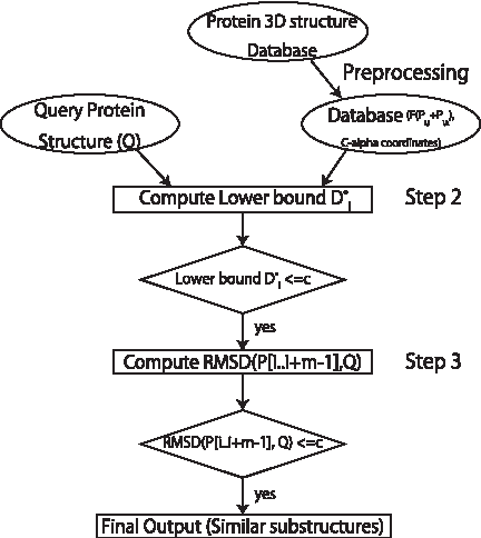
Flow chart of LB3D.

2.5 Preprocessing (Step 1) > Indexing the protein substructures

The process of reading the large number of PDB text files is known to be time consuming and significantly reduces the speed of searching. Moreover, the value of F(P_i,j + P_i,k), where \documentclass{aastex}\usepackage{amsbsy}\usepackage{amsfonts}\usepackage{amssymb}\usepackage{bm}\usepackage{mathrsfs}\usepackage{pifont}\usepackage{stmaryrd}\usepackage{textcomp}\usepackage{portland, xspace}\usepackage{amsmath, amsxtra}\pagestyle{empty}\DeclareMathSizes{10}{9}{7}{6}\begin{document} $$1 \leq j \leq k \leq 6$$ \end{document} , for all positions i in database P are fixed according to the query length m. Therefore, we pre-computed all F(P_i,j + P_i,k) and set an index for all substructures in the database P before performing the computation of D*_i. We can compute all F(P_i,j + P_i,k) for all i in O(N) time. Consequently, all positions i are sorted according to a value of F(P_i,₁ + P_i,₆). Let L represent the list of the sorted i. The list L, F(P_i,j + P_i,k) of all positions i and all C-alpha coordinates are recorded in a binary format file. For 110,799 molecules which contain over 10.1 million substructures, the database expands to 1.1 GBytes after the completion of the preprocessing. The bottleneck for the computational time of preprocessing is the processes of reading the PDB files and writing the database, which is dependent on the file input/output speed. For example, the preprocessing step takes 2,000–3,000 sec for 110,799 molecules, whereas the calculation of all F() and the indexing takes only 10–20 sec. Although the preprocessing needs O(N log N)-time, as shown in the next section, this step is a time-consuming process that is dependent on the input/output speed of the hardware. Moreover, this process does not need to be repeated for a fixed query length m. Thus, the deceleration caused by the preprocessing step is a negligible factor.

2.6 Step 2. Computing the lower bounds

Although computing D*_i is much faster than computing the actual RMSDs, the computational costs of the calculation D*_i for all positions using a huge database (such as the PDB or SCOP) is not possible. By using the binary search algorithm on the sorted list L, we can reduce the computational cost before calculating D*_i for all positions. The binary search algorithm is widely used to find the position which has the key value in a sorted array. According to expression (23), the lower bound for the RMSD is described by only the first and sixth segments as: \documentclass{aastex}\usepackage{amsbsy}\usepackage{amsfonts}\usepackage{amssymb}\usepackage{bm}\usepackage{mathrsfs}\usepackage{pifont}\usepackage{stmaryrd}\usepackage{textcomp}\usepackage{portland, xspace}\usepackage{amsmath, amsxtra}\pagestyle{empty}\DeclareMathSizes{10}{9}{7}{6}\begin{document} \begin{align*} RMSD (P [ i..i + m - 1 ] , Q) \geq \sqrt {\frac {m^{\prime}} {m}} \cdot D (P_{i , 1} + P_{i , 6} , Q_1 + Q_6) \tag {25} \end{align*} \end{document}

where D(P_i,1 + P_i,6, Q₁ + Q₆) represents the |F(P_i,1 + P_i,6) − F(Q₁ + Q₆)|. Let E(P[i.i + m − 1], Q) denote this lower bound.

If \documentclass{aastex}\usepackage{amsbsy}\usepackage{amsfonts}\usepackage{amssymb}\usepackage{bm}\usepackage{mathrsfs}\usepackage{pifont}\usepackage{stmaryrd}\usepackage{textcomp}\usepackage{portland, xspace}\usepackage{amsmath, amsxtra}\pagestyle{empty}\DeclareMathSizes{10}{9}{7}{6}\begin{document} $$RMSD (P [ i..i + m - 1 ] , Q) \leq c$$ \end{document} , expression (25) corresponds to the following expression: \documentclass{aastex}\usepackage{amsbsy}\usepackage{amsfonts}\usepackage{amssymb}\usepackage{bm}\usepackage{mathrsfs}\usepackage{pifont}\usepackage{stmaryrd}\usepackage{textcomp}\usepackage{portland, xspace}\usepackage{amsmath, amsxtra}\pagestyle{empty}\DeclareMathSizes{10}{9}{7}{6}\begin{document} \begin{align*} F (Q_1 + Q_6) - c \cdot \sqrt {\frac {m} {m^{\prime}}} \leq F (P_{i , 1} + P_{i , 6}) \leq F (Q_1 + Q_6) + c \cdot \sqrt {\frac {m} {m^{\prime}}} \tag {26} \end{align*} \end{document}

Therefore, before completing the calculation of all D*_i values, we can find all positions i corresponding to expression (26) by using a binary search algorithm on the sorted list L. Then, after computing D*_i, where i corresponds to expression (26), we filter out dissimilar substructures where the D*_i is greater than the given threshold c before the calculation of actual the RMSD.

2.7 Step 3. Compute the RMSD

The calculation of RMSD(P[i.i + m − 1], Q) is performed for all candidates that passed Step 2. We can then list all similar substructures whose RMSD values are lower than given threshold c.

2.8 Computational time analysis

To analyze the time complexity of the algorithm, we assumed that the structures in the database follow a model called the freely-jointed chain (FJC) model. In the FJC model, we assume that the structures of the chain molecules (in the database) can be considered as random walks in 3D space. This model is a basic and simple model used in molecular physics for chain molecules such as proteins, and is also used for analyzing the average-case (i.e., expected) time complexity of algorithms that deal with chain molecules. Though there are of course many repeated substructures or common substructures in protein databases, the experimental results showed that the behavior of database searching algorithms on PDB reflects the FJC model (Shibuya, 2010a).

According to Shibuya (2010a), the following lemma holds for the lower bound D:

Lemma 1 (Shibuya, 2010a)

For any protein structures P and Q with the same length, the probability \documentclass{aastex}\usepackage{amsbsy}\usepackage{amsfonts}\usepackage{amssymb}\usepackage{bm}\usepackage{mathrsfs}\usepackage{pifont}\usepackage{stmaryrd}\usepackage{textcomp}\usepackage{portland, xspace}\usepackage{amsmath, amsxtra}\pagestyle{empty}\DeclareMathSizes{10}{9}{7}{6}\begin{document} $$\Pr (D (P , Q) \leq c)$$ \end{document} is in \documentclass{aastex}\usepackage{amsbsy}\usepackage{amsfonts}\usepackage{amssymb}\usepackage{bm}\usepackage{mathrsfs}\usepackage{pifont}\usepackage{stmaryrd}\usepackage{textcomp}\usepackage{portland, xspace}\usepackage{amsmath, amsxtra}\pagestyle{empty}\DeclareMathSizes{10}{9}{7}{6}\begin{document} $$O (c / N^{0.5})$$ \end{document} , where N is the length of P (or Q) under the assumption that either P or Q follows the FJC model.

We obtained a similar result on the lower bound E(P, Q) as follows:

Theorem 1

For any protein structures P and Q of the same length, the probability \documentclass{aastex}\usepackage{amsbsy}\usepackage{amsfonts}\usepackage{amssymb}\usepackage{bm}\usepackage{mathrsfs}\usepackage{pifont}\usepackage{stmaryrd}\usepackage{textcomp}\usepackage{portland, xspace}\usepackage{amsmath, amsxtra}\pagestyle{empty}\DeclareMathSizes{10}{9}{7}{6}\begin{document} $$\Pr (E (P [ i..i + m - 1 ] , Q \leq c)$$ \end{document} is in \documentclass{aastex}\usepackage{amsbsy}\usepackage{amsfonts}\usepackage{amssymb}\usepackage{bm}\usepackage{mathrsfs}\usepackage{pifont}\usepackage{stmaryrd}\usepackage{textcomp}\usepackage{portland, xspace}\usepackage{amsmath, amsxtra}\pagestyle{empty}\DeclareMathSizes{10}{9}{7}{6}\begin{document} $$O (c / N^{0.5})$$ \end{document} , where N is the length of P (or Q), under the assumption that either P or Q follows the FJC model.

Proof. Consider a protein structure S of length 6m′ that follows the FJC model. Let a_i denote \documentclass{aastex}\usepackage{amsbsy}\usepackage{amsfonts}\usepackage{amssymb}\usepackage{bm}\usepackage{mathrsfs}\usepackage{pifont}\usepackage{stmaryrd}\usepackage{textcomp}\usepackage{portland, xspace}\usepackage{amsmath, amsxtra}\pagestyle{empty}\DeclareMathSizes{10}{9}{7}{6}\begin{document} $$S [ i + 1 ] - S [ i ]$$ \end{document} . Note that vectors a_i are assumed to be random vectors that are independent to each other in the FJC model. Then \documentclass{aastex}\usepackage{amsbsy}\usepackage{amsfonts}\usepackage{amssymb}\usepackage{bm}\usepackage{mathrsfs}\usepackage{pifont}\usepackage{stmaryrd}\usepackage{textcomp}\usepackage{portland, xspace}\usepackage{amsmath, amsxtra}\pagestyle{empty}\DeclareMathSizes{10}{9}{7}{6}\begin{document} $$F (S [ i..m^{\prime} ] , S [ 5m^{\prime} + 1..6m^{\prime} ])$$ \end{document} can be described as follows: \documentclass{aastex}\usepackage{amsbsy}\usepackage{amsfonts}\usepackage{amssymb}\usepackage{bm}\usepackage{mathrsfs}\usepackage{pifont}\usepackage{stmaryrd}\usepackage{textcomp}\usepackage{portland, xspace}\usepackage{amsmath, amsxtra}\pagestyle{empty}\DeclareMathSizes{10}{9}{7}{6}\begin{document} \begin{align*} F (S [ 1..m^{\prime} ] , S [ 5m^{\prime} + 1..6m^{\prime}]) & = \frac {1} {2m^{\prime}} \left\{\sum_{i = 1}^{m^{\prime}} (S [ 1 ] + \sum_{j = 1}^{i - 1} a_j) - \sum_{i = 5m^{\prime} + 1}^{6m^{\prime}} (S [ 1 ] + \sum_{j = 1}^{i - 1} a_j) \right\} \\ & = - \frac {1} {2} \left\{\sum_{i = 1}^{m^{\prime}} \frac {1} {m^{\prime}} a_i + \sum_{i = m^{\prime} + 1}^{5m^{\prime}} a_i + \sum_{i = 5m^{\prime} + 1}^{6m^{\prime} - 1} \frac {6m^{\prime} - i} {m^{\prime}} a_i \right\} \tag {27} \end{align*} \end{document}

Let b_i denote \documentclass{aastex}\usepackage{amsbsy}\usepackage{amsfonts}\usepackage{amssymb}\usepackage{bm}\usepackage{mathrsfs}\usepackage{pifont}\usepackage{stmaryrd}\usepackage{textcomp}\usepackage{portland, xspace}\usepackage{amsmath, amsxtra}\pagestyle{empty}\DeclareMathSizes{10}{9}{7}{6}\begin{document} $$i \cdot a_i / m^{\prime}$$ \end{document} if \documentclass{aastex}\usepackage{amsbsy}\usepackage{amsfonts}\usepackage{amssymb}\usepackage{bm}\usepackage{mathrsfs}\usepackage{pifont}\usepackage{stmaryrd}\usepackage{textcomp}\usepackage{portland, xspace}\usepackage{amsmath, amsxtra}\pagestyle{empty}\DeclareMathSizes{10}{9}{7}{6}\begin{document} $$i \leq m^{\prime}$$ \end{document} , a_i if \documentclass{aastex}\usepackage{amsbsy}\usepackage{amsfonts}\usepackage{amssymb}\usepackage{bm}\usepackage{mathrsfs}\usepackage{pifont}\usepackage{stmaryrd}\usepackage{textcomp}\usepackage{portland, xspace}\usepackage{amsmath, amsxtra}\pagestyle{empty}\DeclareMathSizes{10}{9}{7}{6}\begin{document} $$m^{\prime} < i \leq 5 m^{\prime}$$ \end{document} , and \documentclass{aastex}\usepackage{amsbsy}\usepackage{amsfonts}\usepackage{amssymb}\usepackage{bm}\usepackage{mathrsfs}\usepackage{pifont}\usepackage{stmaryrd}\usepackage{textcomp}\usepackage{portland, xspace}\usepackage{amsmath, amsxtra}\pagestyle{empty}\DeclareMathSizes{10}{9}{7}{6}\begin{document} $$(6m^{\prime} - i) \cdot a_i / m^{\prime}$$ \end{document} if \documentclass{aastex}\usepackage{amsbsy}\usepackage{amsfonts}\usepackage{amssymb}\usepackage{bm}\usepackage{mathrsfs}\usepackage{pifont}\usepackage{stmaryrd}\usepackage{textcomp}\usepackage{portland, xspace}\usepackage{amsmath, amsxtra}\pagestyle{empty}\DeclareMathSizes{10}{9}{7}{6}\begin{document} $$i > 5m^{\prime}$$ \end{document} . Let z_i denote the z coordinate of b_i. Let \documentclass{aastex}\usepackage{amsbsy}\usepackage{amsfonts}\usepackage{amssymb}\usepackage{bm}\usepackage{mathrsfs}\usepackage{pifont}\usepackage{stmaryrd}\usepackage{textcomp}\usepackage{portland, xspace}\usepackage{amsmath, amsxtra}\pagestyle{empty}\DeclareMathSizes{10}{9}{7}{6}\begin{document} \begin{align*} M_{m^{\prime}} = \frac {1} {\sqrt {\sum \limits_{i = 1}^{6m^{\prime}} {\rm var} (z_i)}^{2 + \delta}} \sum_{i = 1}^{6m^{\prime}} \langle \mid z_i - \langle z_i \rangle \rangle^{2 + \delta} \tag {28} \end{align*} \end{document}

where δ is some positive constant. According to Lyapunov's central limit theorem (Kallenberg, 1997), the distribution of \documentclass{aastex}\usepackage{amsbsy}\usepackage{amsfonts}\usepackage{amssymb}\usepackage{bm}\usepackage{mathrsfs}\usepackage{pifont}\usepackage{stmaryrd}\usepackage{textcomp}\usepackage{portland, xspace}\usepackage{amsmath, amsxtra}\pagestyle{empty}\DeclareMathSizes{10}{9}{7}{6}\begin{document} $$\sum\nolimits_{i = 1}^{6m^{\prime}} z_i$$ \end{document} converges to the Gaussian distribution, if \documentclass{aastex}\usepackage{amsbsy}\usepackage{amsfonts}\usepackage{amssymb}\usepackage{bm}\usepackage{mathrsfs}\usepackage{pifont}\usepackage{stmaryrd}\usepackage{textcomp}\usepackage{portland, xspace}\usepackage{amsmath, amsxtra}\pagestyle{empty}\DeclareMathSizes{10}{9}{7}{6}\begin{document} $$M_{m^{\prime}}$$ \end{document} converges to 0 as m′ grows to infinity for some δ such that \documentclass{aastex}\usepackage{amsbsy}\usepackage{amsfonts}\usepackage{amssymb}\usepackage{bm}\usepackage{mathrsfs}\usepackage{pifont}\usepackage{stmaryrd}\usepackage{textcomp}\usepackage{portland, xspace}\usepackage{amsmath, amsxtra}\pagestyle{empty}\DeclareMathSizes{10}{9}{7}{6}\begin{document} $$\delta > 0$$ \end{document} . It can be proved with the following inequality: \documentclass{aastex}\usepackage{amsbsy}\usepackage{amsfonts}\usepackage{amssymb}\usepackage{bm}\usepackage{mathrsfs}\usepackage{pifont}\usepackage{stmaryrd}\usepackage{textcomp}\usepackage{portland, xspace}\usepackage{amsmath, amsxtra}\pagestyle{empty}\DeclareMathSizes{10}{9}{7}{6}\begin{document} \begin{align*} M_{m^{\prime}} = \frac {1} {\sqrt {\sum \limits_{i = 1}^{6m^{\prime}} \langle \mid z_i \mid \rangle^2}^{2 + \delta}} \sum_{i = 1}^{6m^{\prime}} \langle \mid z_i \mid \rangle^{2 + \delta} \leq \left\{\sum_{i = 1}^{6m^{\prime}} \langle \mid z_i \mid \rangle^2 \right\}^{- \delta / 2} = \left\{\frac {14} {9} m^{\prime} + \frac {1} {9m^{\prime}} \right\}^{- \delta / 2} \to 0 \quad (m^{\prime} \to \infty) \tag {29} \end{align*} \end{document}

This means that \documentclass{aastex}\usepackage{amsbsy}\usepackage{amsfonts}\usepackage{amssymb}\usepackage{bm}\usepackage{mathrsfs}\usepackage{pifont}\usepackage{stmaryrd}\usepackage{textcomp}\usepackage{portland, xspace}\usepackage{amsmath, amsxtra}\pagestyle{empty}\DeclareMathSizes{10}{9}{7}{6}\begin{document} $$F (S [ 1..m^{\prime} ] , S [ 5m^{\prime} + 1..6m^{\prime} ])$$ \end{document} converges to the Gaussian distribution in 3D space as m′ grows to infinity. The same discussion can be performed for the other two axes x and y. The variance of \documentclass{aastex}\usepackage{amsbsy}\usepackage{amsfonts}\usepackage{amssymb}\usepackage{bm}\usepackage{mathrsfs}\usepackage{pifont}\usepackage{stmaryrd}\usepackage{textcomp}\usepackage{portland, xspace}\usepackage{amsmath, amsxtra}\pagestyle{empty}\DeclareMathSizes{10}{9}{7}{6}\begin{document} $$F (S [ 1..m^{\prime} ] , S [ 5m^{\prime} + 1..6m^{\prime} ])$$ \end{document} is computed as follows. \documentclass{aastex}\usepackage{amsbsy}\usepackage{amsfonts}\usepackage{amssymb}\usepackage{bm}\usepackage{mathrsfs}\usepackage{pifont}\usepackage{stmaryrd}\usepackage{textcomp}\usepackage{portland, xspace}\usepackage{amsmath, amsxtra}\pagestyle{empty}\DeclareMathSizes{10}{9}{7}{6}\begin{document} \begin{align*} {\rm var} (F (S [ 1..m^{\prime} ] , S [ 5m^{\prime} + 1..6m^{\prime} ]) = \langle \mid F (S [ 1..m^{\prime} ] , S [ 5m^{\prime} + 1..6m^{\prime} ] \mid^2 \rangle = \frac {7} {6} m^{\prime} + \frac {1} {12m^{\prime}} \approx \frac {7} {6} m^{\prime} \tag {30} \end{align*} \end{document}

This means that the distribution of \documentclass{aastex}\usepackage{amsbsy}\usepackage{amsfonts}\usepackage{amssymb}\usepackage{bm}\usepackage{mathrsfs}\usepackage{pifont}\usepackage{stmaryrd}\usepackage{textcomp}\usepackage{portland, xspace}\usepackage{amsmath, amsxtra}\pagestyle{empty}\DeclareMathSizes{10}{9}{7}{6}\begin{document} $$F (S [ 1..m^{\prime} ] , S [ 5m^{\prime} + 1..6m^{\prime} ])$$ \end{document} is the same as the distribution of random walks of length \documentclass{aastex}\usepackage{amsbsy}\usepackage{amsfonts}\usepackage{amssymb}\usepackage{bm}\usepackage{mathrsfs}\usepackage{pifont}\usepackage{stmaryrd}\usepackage{textcomp}\usepackage{portland, xspace}\usepackage{amsmath, amsxtra}\pagestyle{empty}\DeclareMathSizes{10}{9}{7}{6}\begin{document} $$7 m^{\prime} / 6$$ \end{document} , if m′ is large enough. Hence, we can deduce that the probability that \documentclass{aastex}\usepackage{amsbsy}\usepackage{amsfonts}\usepackage{amssymb}\usepackage{bm}\usepackage{mathrsfs}\usepackage{pifont}\usepackage{stmaryrd}\usepackage{textcomp}\usepackage{portland, xspace}\usepackage{amsmath, amsxtra}\pagestyle{empty}\DeclareMathSizes{10}{9}{7}{6}\begin{document} \begin{align*} F (Q_1 + Q_6) - c \cdot \sqrt {\frac {m} {m^{\prime}}} \leq F (P_{i , 1} + P_{i , 6}) \leq F (Q_1 + Q_6) + c \cdot \sqrt {\frac {m} {m^{\prime}}} \tag {31} \end{align*} \end{document}

holds is only in \documentclass{aastex}\usepackage{amsbsy}\usepackage{amsfonts}\usepackage{amssymb}\usepackage{bm}\usepackage{mathrsfs}\usepackage{pifont}\usepackage{stmaryrd}\usepackage{textcomp}\usepackage{portland, xspace}\usepackage{amsmath, amsxtra}\pagestyle{empty}\DeclareMathSizes{10}{9}{7}{6}\begin{document} $$O (c / \sqrt{m})$$ \end{document} , if either P or Q follows the FJC model, with the same discussion as in Shibuya (2010a). Consequently, we conclude that the probability \documentclass{aastex}\usepackage{amsbsy}\usepackage{amsfonts}\usepackage{amssymb}\usepackage{bm}\usepackage{mathrsfs}\usepackage{pifont}\usepackage{stmaryrd}\usepackage{textcomp}\usepackage{portland, xspace}\usepackage{amsmath, amsxtra}\pagestyle{empty}\DeclareMathSizes{10}{9}{7}{6}\begin{document} $$\Pr (E (P [ i..i + m - 1 ] , Q) \leq c)$$ \end{document} is in \documentclass{aastex}\usepackage{amsbsy}\usepackage{amsfonts}\usepackage{amssymb}\usepackage{bm}\usepackage{mathrsfs}\usepackage{pifont}\usepackage{stmaryrd}\usepackage{textcomp}\usepackage{portland, xspace}\usepackage{amsmath, amsxtra}\pagestyle{empty}\DeclareMathSizes{10}{9}{7}{6}\begin{document} $$O (c / \sqrt{m})$$ \end{document} , where N is the length of P (or Q) under the assumption that either P or Q follows the FJC model. ▪

According to Shibuya (2010a), the following lemma also holds for the lower bound LB_i,1:

Lemma 2 (Shibuya, 2010a)

For any protein structures P and Q of the same length, the probability \documentclass{aastex}\usepackage{amsbsy}\usepackage{amsfonts}\usepackage{amssymb}\usepackage{bm}\usepackage{mathrsfs}\usepackage{pifont}\usepackage{stmaryrd}\usepackage{textcomp}\usepackage{portland, xspace}\usepackage{amsmath, amsxtra}\pagestyle{empty}\DeclareMathSizes{10}{9}{7}{6}\begin{document} $$\Pr (LB_{i , 1} (P , Q) \leq c)$$ \end{document} is in \documentclass{aastex}\usepackage{amsbsy}\usepackage{amsfonts}\usepackage{amssymb}\usepackage{bm}\usepackage{mathrsfs}\usepackage{pifont}\usepackage{stmaryrd}\usepackage{textcomp}\usepackage{portland, xspace}\usepackage{amsmath, amsxtra}\pagestyle{empty}\DeclareMathSizes{10}{9}{7}{6}\begin{document} $$O (c / N^{1.5})$$ \end{document} where N is the length of P (or Q), under the assumption that either P or Q follows the FJC model.

It is easy to see that the following corollary holds for our lower bound D*_i:

Corollary 1

For any protein structures P and Q, the probability \documentclass{aastex}\usepackage{amsbsy}\usepackage{amsfonts}\usepackage{amssymb}\usepackage{bm}\usepackage{mathrsfs}\usepackage{pifont}\usepackage{stmaryrd}\usepackage{textcomp}\usepackage{portland, xspace}\usepackage{amsmath, amsxtra}\pagestyle{empty}\DeclareMathSizes{10}{9}{7}{6}\begin{document} $$\Pr (D^*{}_1 (P , Q) \leq c)$$ \end{document} is in \documentclass{aastex}\usepackage{amsbsy}\usepackage{amsfonts}\usepackage{amssymb}\usepackage{bm}\usepackage{mathrsfs}\usepackage{pifont}\usepackage{stmaryrd}\usepackage{textcomp}\usepackage{portland, xspace}\usepackage{amsmath, amsxtra}\pagestyle{empty}\DeclareMathSizes{10}{9}{7}{6}\begin{document} $$O (c / \sqrt{N})$$ \end{document} where N is the length of P (or Q) under the assumption that either P or Q follows the FJC model.

Proof. According to the definition of D*_i in expression (24), \documentclass{aastex}\usepackage{amsbsy}\usepackage{amsfonts}\usepackage{amssymb}\usepackage{bm}\usepackage{mathrsfs}\usepackage{pifont}\usepackage{stmaryrd}\usepackage{textcomp}\usepackage{portland, xspace}\usepackage{amsmath, amsxtra}\pagestyle{empty}\DeclareMathSizes{10}{9}{7}{6}\begin{document} $$D^*{}_i (P , Q) \geq LB_{i , 1} (P , Q)$$ \end{document} holds. Consequently, \documentclass{aastex}\usepackage{amsbsy}\usepackage{amsfonts}\usepackage{amssymb}\usepackage{bm}\usepackage{mathrsfs}\usepackage{pifont}\usepackage{stmaryrd}\usepackage{textcomp}\usepackage{portland, xspace}\usepackage{amsmath, amsxtra}\pagestyle{empty}\DeclareMathSizes{10}{9}{7}{6}\begin{document} $$\Pr (D^*{}_1 (P , Q) \leq c) < \Pr (LB_{i , 1} (P , Q) \leq c)$$ \end{document} holds, from which we can deduce that \documentclass{aastex}\usepackage{amsbsy}\usepackage{amsfonts}\usepackage{amssymb}\usepackage{bm}\usepackage{mathrsfs}\usepackage{pifont}\usepackage{stmaryrd}\usepackage{textcomp}\usepackage{portland, xspace}\usepackage{amsmath, amsxtra}\pagestyle{empty}\DeclareMathSizes{10}{9}{7}{6}\begin{document} $$\Pr (D^*{}_1 (P , Q) \leq c)$$ \end{document} is also in \documentclass{aastex}\usepackage{amsbsy}\usepackage{amsfonts}\usepackage{amssymb}\usepackage{bm}\usepackage{mathrsfs}\usepackage{pifont}\usepackage{stmaryrd}\usepackage{textcomp}\usepackage{portland, xspace}\usepackage{amsmath, amsxtra}\pagestyle{empty}\DeclareMathSizes{10}{9}{7}{6}\begin{document} $$O (c / N^{1.5})$$ \end{document} , based on Lemma 2. ▪

The time complexity of our algorithm can be analyzed as follows (based on the above discussion). In the preprocessing step, we need only O(N) time for obtaining F() values, but need O(N log N) time to sort them to compute the sorted list L. In Step 2, we require O(log N) time for the binary search. After binary searching, we obtain O(N/m^0.5) candidates, according to Theorem 1. For these candidates, we compute the D*_i values, which takes only O(1) for each. After computing the D*_i values, the number of remaining candidates is only in O(N/m^1.5), according to Corollary 1. In Step 3, we compute the RMSD for all the remaining candidates, which requires O(m) time for each. Overall, the presented algorithm achieves O(m + N/m^0.5) average-case time complexity, after O(N log N) preprocessing, because the term O(log N) can be ignored. Note that the worst-case query time complexity is still O(Nm).

3 Results and Discussion

3.1 Computational experiments on the SCOP1.75 database

To test the performance of the new algorithm, we used the SCOP database (Andreeva et al., 2008) release 1.75 (denoted as SCOP1.75), which contains 110,799 domains with a total of 20,429,263 C-alpha coordinates. We randomly selected 100 domains from SCOP1.75 as query domains for this experiment. These 100 domains contained a total of 6,710–22,692 substructures depending on the length of substructures (10–200). All the 3D coordinates are taken from the ASTRAL database (Chandonia et al., 2004).

The goal is to execute the exhaustive search of similar substructures much faster than known algorithms. We compared three algorithms (Naive, A3, and LB3D). Naive performs an exhaustive calculation of the RMSD against all substructures of the database without any filtering. The computational time of Naive is known as O(Nm). A3 is the best known algorithm, reported as an O(N)-time algorithm by Shibuya. In this experiment, to reduce computational costs, A3 uses the indexed data which consists of a sorted list of all substructures according to the value of F(P_i,₁ + P_i,₂) before computing all the lower bounds for the RMSD (expression (3)). LB3D denotes our new algorithm described above and is a faster O(m + N/m^0.5) algorithm. There are no parameters that need optimization in the algorithms. LB3D was implemented in ANSI C and runs on standard Linux OS. We used a Linux computing system (Intel Xeon E5506 CPU of 2.13 GHz and 12 GByte memory) for the following experiments.

We compared these three algorithms among various query lengths and a fixed threshold (c = 1.0 Å). Table 1 summarizes the results of the experiments on SCOP1.75. All three algorithms performed an exhaustive search. Therefore, the average number of similar substructures that were found by each algorithm (“#Hits”) are always the same. This indicates that there was no requirement to compare the qualities of these search methods. As shown in the row of “Time” and “Time/1M,” LB3D clearly performed faster than the other two algorithms: about 1.8–41 times faster than A3 and 2.3–1536 times faster than Naive. In particular, for the medium-long query (over 40 residues), LB3D is at least 18.4 and 514 times faster than A3 and Naive, respectively.

Table 1.

Results of the Computational Experiments

Query length	10	20	40	60	80	100	120	140	160	180	200
#Query^a	222692	21692	19692	17692	15692	13692	11826	10236	8830	7698	6710
#Substructures^b	19432226	18326890	16139532	14015367	12009140	10173524	8606303	7292124	6179494	5241111	4433040
#Hits^c	495394.6	8048.6	62.6	49.7	44.2	40.1	37.6	35.3	33.6	31.5	29.0
#Hits/1M^d	25493.5	439.2	3.9	3.5	3.7	3.9	4.4	4.8	5.4	6.0	6.5
A3^e
#Checked^f	19280552.8	5766560.1	2267443.1	636246.1	327470.1	203795.0	128116.7	107096.6	93159.1	76184.0	63815.1
#Checked/1M^g	992194.8	314650.2	140490.0	45396.3	27268.4	20031.9	14886.4	14686.6	15075.5	14535.9	14395.3
#Checked/Hits^h	38.9	716.5	36233.0	12812.6	7405.1	5084.9	3409.9	3034.7	2769.4	2417.2	2203.9
Time(sec)ⁱ	14.481	7.845	4.755	1.803	1.168	0.872	0.620	0.583	0.564	0.504	0.460
Time/1M(sec)^j	0.745	0.428	0.295	0.129	0.097	0.086	0.072	0.080	0.091	0.096	0.104
LB3D^k
#Checked	7312183.3	387860.3	5393.5	216.0	183.3	192.3	209.9	233.8	246.7	276.4	276.9
#Checked/1M	376291.6	21163.5	334.2	15.4	15.3	18.9	24.4	32.1	39.9	52.7	62.5
#Checked/Hits	14.8	48.2	86.2	4.4	4.1	4.8	5.6	6.6	7.3	8.8	9.6
Time(sec)	8.146	0.876	0.114	0.069	0.058	0.047	0.040	0.033	0.029	0.024	0.020
Time/1M(sec)	0.419	0.048	0.007	0.005	0.005	0.005	0.005	0.005	0.005	0.005	0.004
Naive^l
Time(sec)	18.795	23.279	31.849	35.590	38.839	38.591	37.876	36.392	34.554	32.273	29.967
Time/1M(sec)	0.967	1.270	1.973	2.539	3.234	3.793	4.401	4.991	5.592	6.158	6.760

The number of query substructures which were obtained from the randomly selected 100 domains.

The total number of substructures in the database corresponding to the query length.

The average number of substructures whose RMSDs to queries consisted of 100 random domains, and were lower than 1.0 Å.

The number of “Hits” per one million (1M) substructures.

Algorithm 3, O(N) algorithm, using expression (9).

The average number of substructures whose actual RMSDs were computed. It also means that the average number of substructures whose lower bounds for RMSDs are lower than the given threshold (1.0 Å).

The number of “Checked” per 1M substructures.

The ratio of the average number of “#Checked” against “#Hits.” This represents the average number of substructures whose actual RMSDs were computed per one actual similar substructure.

The average computation time, excluding the preprocessing step.

The average computation time per 1M substructures.

Our new O(m + N/m^0.5) algorithm, using the new lower bound (expression (24)).

O(Nm) algorithm; computing the RMSDs for all substructures.

The rows of “#Checked” and “#Checked/1M” indicated the number of RMSDs of the substructures that were not filtered by lower bounds and were computed per one query substructure. It is equivalent to the efficiency of the filtering with the lower bound used in the algorithm. The calculation of the RMSDs is computationally more expensive than that of the lower bounds for the RMSD. The time to find all similar substructures whose RMSDs to the query are at most given threshold is directly dependent on the number of checked substructures; therefore, lowering the number of RMSDs will accelerate the search. Examination of the speed (“Time” and “Time/1M”) by comparison of “#Check/1M” in LB3D and A3 indicated that the use of D*_i provides a significant advantage in the filtering of dissimilar substructures.

Interesting results were observed when we focused on the limitation of the efficiency of the filtering with the lower bound. Here, the average number of checked substructures per one substructure whose RMSD is lower than the given threshold (1.0 Å) was denoted as “#Checked/Hits.” For example, the “#Checked/Hits” of LB3D indicates only 4.1–9.6 when the query lengths were 60–200. This indicated that, if the computational cost of filtering is not improved, there is modest room (at most 4.1–9.6 times faster than LB3D) for improving LB3D-like algorithms. In contrast, “#Checked/Hits” of LB3D for a small-to-medium query (especially when the lengths were 20 and 40) showed a significantly poorer performance than the results obtained using the other query lengths. For these small queries associated with two or three secondary structure elements (SSEs), we are considering ways to improve the performance by using other methods such as comparing each SSE or using the orientation of the SSEs.

Moreover, as shown in Table 1, the query length does not affect the “Time/1M” of both A3 and LB3D. On the other hand, in the Naive O(Nm) algorithm, computational cost (“Time/1M”) clearly increased as the length of the query increased.

As mentioned above, the performance of the speed is directly dependent on the performance of the filtering approach, which corresponds to Step 2 of Figure 2. To evaluate the ability of filtering dissimilar substructures, a number of checked substructures at various thresholds (0.2–5.0Å) and query lengths (10–200) were analyzed by comparison of LB3D and A3. Figure 3 shows the results of A3 and LB3D using different query lengths and thresholds. LB3D can filter out over 90% of the substructures from the database when the query length is >60 and the threshold is lower than 4.0 Å. In comparison to A3, LB3D performed significantly better at filtering queries of any length and threshold values. Surprisingly, even when examining small queries (length = 10, 20), LB3D computed actual RMSDs of only 38% and 2% of the database when the threshold c was set to 1.0 Å.

Fig. 3.

Average number of checked RMSDs of substructures per 1M substructures of the database (SCOP1.75). (A) Results of Algorithm 3. (B) Results of LB3D.

The advantages of the new algorithm suggest that the algorithm has further applications in various fields: (1) LB3D can find all AFPs among a huge database and filter out dissimilar protein structures before computing all structural alignments. Therefore, the speed of searching for a protein structure which has the same fold could be significantly increased using the new algorithm. (2) For protein-protein docking, similar 3D patterns of protein-protein interactions can be found by the algorithm. Even if the substructures of the query or database are not sequentially connected, the new lower bound (expression (24)) can be applied. (3) For protein structure prediction, the algorithm can detect structural conservations by searching all AFPs.

4 Conclusion

In this article, we have developed a new substructure search algorithm, LB3D, which is based on a new lower bound for the RMSD value (expression (24)). We proved that the new algorithm is an O(m + N/m^0.5) average-case time query algorithm after O(N log N)-time preprocessing. We showed that the new algorithm is significantly faster than the best-known O(N) algorithm (Algorithm 3) and the most common O(Nm) algorithm (Naive). We attribute the search speed of LB3D to the number of substructures that are filtered as dissimilar substructures by using a lower bound for the RMSD. LB3D can efficiently eliminate dissimilar substructures before computing the actual RMSDs, even when small queries (10–40) or large thresholds (∼5 Å) are used. Thus, LB3D is a useful tool for performing an exhaustive search using a huge database to find all similar substructures.

Footnotes

Acknowledgments

We thank Mr. M. Oosawa for valuable cooperation. This research was partially supported by the Ministry of Education, Science, Sports and Culture, Grant-in-Aid for Young Scientists (B), 22700314, 2010–2011.

Disclosure Statement

No competing financial interests exist.

References

Altschul

S.F.

, Madden

T.L.

, Schäffer

A.A.

et al. 1997. Gapped BLAST and PSI-BLAST: a new generation of protein database search programs. Nucleic Acids Res., 25:3389–3402.

Andreeva

, Howorth

, Chandonia

J.-M.

et al. 2008. Data growth and its impact on the SCOP database: new developments. Nucleic Acids Res, 36:D419–D425.

Berman

H.M.

, Westbrook

, Feng

et al. 2000. The Protein Data Bank. Nucleic Acids Res, 28:235–242.

Betts

M.J.

, Guigó

, Agarwal

et al. 2001. Exon structure conservation despite low sequence similarity: a relic of dramatic events in evolution? EMBO J., 20:5354–5360.

Chandonia

J.-M.

, Hon

, Walker

N.S.

et al. 2004. The ASTRAL Compendium in 2004. Nucleic Acids Res., 32:D189–D192.

Diamond

1998. A note on the rotational superposition problem. Acta Cryst. A, 44:211–216.

Gao

, Zaki

M.J.

2005. PSIST: indexing protein structures using suffix trees. Proc. Comput. Syst. Bioinform. Conf. 2005, 212–222.

Holm

, Sander

1993. Protein structure comparison by alignment of distance matrices. J. Mol. Biol, 233:123–138.

Kabsch

1976. A solution for the best rotation to relate two sets of vectors. Acta Cryst. A, 32:922–923.

10.

Kallenberg

1997. Foundations of Modern Probability. Springer-Verlag: New York.

11.

Lathrop

R.H.

1994. The protein threading problem with sequence amino acid interaction preferences is NP-complete. Prot. Eng, 7:1059–1068.

12.

Ortiz

A.R.

, Strauss

C.E.M.

, Olmea

2002. MAMMOTH (MAtching Molecular Models Obtained from THeory): an automated method for model comparison. Prot. Sci, 11:2606–2621.

13.

Shibuya

2010a. Searching protein 3-D structures in linear time. J. Comput. Biol., 17:203–219.

14.

Shibuya

2010b. Searching protein 3-D structures in faster than linear time. J. Comput. Biol., 17:593–602.

15.

Shindyalov

I.N.

, Bourne

P.E.

1998. Protein structure alignment by incremental combinatorial extension (CE) of the optimal path. Prot. Eng., 11:739–747.

16.

Umeyama

1991. Least-square estimation of transformation parameters between two point patterns. IEEE Trans. Pattern Anal. Mach. Intell., 13:376–380.

17.

Zhang

, Skolnick

2005. TM-align: a protein structure alignment algorithm based on the TM-score. Nucleic Acids Res, 33:2302–2309.

18.

Zhu

, Weng

2005. FAST: a novel protein structure alignment algorithm. Proteins, 58:618–627.