
Abstract
Abstract
Gene translation is a central process in all living organism with important ramifications to almost every biomedical field. Previous systems evolutionary studies in the field have demonstrated that in many organisms coding sequence features undergo selection to optimize this process. In the current study, we report for the first time analytical proofs related to the various aspects of this process and its optimality. Among our results we show that coding sequences with mono- tonic increasing profiles of translation efficiency (i.e., with slower codons near the 5′UTR), mathematically optimize ribosomal allocation by minimizing the number of ribosomes needed for translating a codon per time unit. Thus, the genomic translation efficiency profile reported in previous studies for many organisms is optimal in this sense. In addition, we show that improving translation efficiency of a codon in a gene may result in a decrease in the translation rate of other genes, demonstrating that the relation between codon bias and protein translation rate is less trivial than was assumed before. Based on these observations we describe an efficient heuristic for designing coding sequences with specific translation efficiency and minimal ribosomal allocation for heterologous gene expression. We demonstrate how this heuristic can be used in biotechnology for engineering a heterologous gene before expressing it in a new host.
1. Introduction
In recent years many systems biology studies have dealt with questions related to the process of gene translation (Kudla et al., 2009; Drummond and Wilke, 2009; Cannarozzi et al., 2010; Kurt and Michael, 2010; Tuller et al., 2010a,b; Taniguchi et al., 2010; Uemura et al., 2010; Reuveni et al., 2011; Plotkin and Kudla, 2010).
A large portion of these studies were based on large-scale measurements of this process generated by new technologies that have maturated recently (Arava et al., 2003; Newman et al., 2006; Kudla et al., 2009; Ingolia et al., 2009; Welch et al., 2009; Taniguchi et al., 2010; Uemura et al., 2010; Vogel et al., 2010). However, the systematic study of translation is relative new compared to the study of transcription and the field includes many fundamental open questions related to the cellular and coding sequence features that affect its efficiency (Kudla et al., 2009; Welch et al., 2009; Tuller et al., 2010b; Plotkin and Kudla, 2010).
For example, the fact that different codons may have different translation efficiencies has been known for a few decades (Ikemura, 1982; Sharp and Li, 1987; Duret and Mouchiroud, 1999). Based on this observation, it was suggested that a gene's codon composition can affect protein levels (Ikemura, 1982; Sharp and Li, 1987; Duret and Mouchiroud, 1999); thus, measures of the codon bias of a gene can be used for estimating its expression levels or protein abundance (Sharp and Li, 1987; Comeron and Aguad, 1998).
Recently, systems biology studies that were based on large-scale genomic data and cellular measurements have demonstrated that the order of codon, and not only their composition, may also significantly influence the efficiency of translation (Cannarozzi et al., 2010; Kurt and Michael, 2010; Tuller et al., 2010a; Reuveni et al., 2011). Specifically, it was shown that in many species, a “ramp” of codons with lower translation rate tends to appear in the first 30–50 codons of the mRNA. It was suggested that this systematic trend serves as a late stage of translation initiation, forming a means to reduce ribosomal traffic jams, thus minimizing the cost of protein expression by reducing the ribosomal densities over the mRNA sequences (Kurt and Michael, 2010; Tuller et al., 2010a; Plotkin and Kudla, 2010).
In addition, over the years, several mathematical models based on physical and stochastic properties of the translation process were suggested and studied with the intention of mapping and quantifying different factors that could influence translation efficiency from a mathematical point of view. However, these factors were mainly analyzed using computer simulations (MacDonald et al., 1968; Heinrich and Rapoport, 1980; Zhang et al., 1994; Shaw et al., 2003; Reuveni et al., 2011).
In this study, we focus on the elongation stage and on the interaction between the initiation and the elongation, providing analytical proofs to some of the results previous reported in studies based on systems biology analysis. These observed properties were analyzed in this article for a pool with an infinite number of ribosomes, unless stated otherwise.
Next, we describe a method that uses these translation properties to develop an approach for controlling translation efficiency of heterologous genes by manipulating their codons efficiency with the help of synonymous mutations. The implementation of this heuristic can have various biotechnological applications (Gustafsson et al., 2004; Wenzel and Müller, 2005; Burgess-Brown et al., 2008; Welch et al., 2009; Mueller et al., 2010; Thomas and Ming-Qun, 2011).
The rest of the article is organized as follows: in Sections 2.1, 4.1, and 4.2, we provide some details of the analyzed mathematical models in the study. In Section 4.4, we provide analytical proofs related to properties of translation, which are followed with demonstrations in Sections 2.2, 2.3, and 2.5. Sections 2.6 and 2.7 describe an approach for controlling translation rate of a gene, while Sections 2.7 and 4.6 demonstrate the applications of this method on the human gene insulin. The Discussion includes some implications of the results reported in this study and future directions. All details of the proofs appear in the Methods and Proofs section, and some additional proofs appear in Appendix B.
2. Results
2.1. Translation models that are sensitive to the order of codons
Over the years, several mathematical models for describing translation have been suggested. In this study, we focus on models that can incorporate several important physical properties of the translation process, such as the volume of the ribosome, the different translation rate of each type of codons and their order on the mRNA. Initiation time was shown to depend on several features, such as the number of free ribosomes in the cell and features of the 5′UTR, such as the folding energy at the beginning of the ORF (Kozak, 1987; Kudla et al., 2009); therefore, this factor can differ among genes and hosts, thus should be parameterized in order to study its influence on the overall translation efficiency.
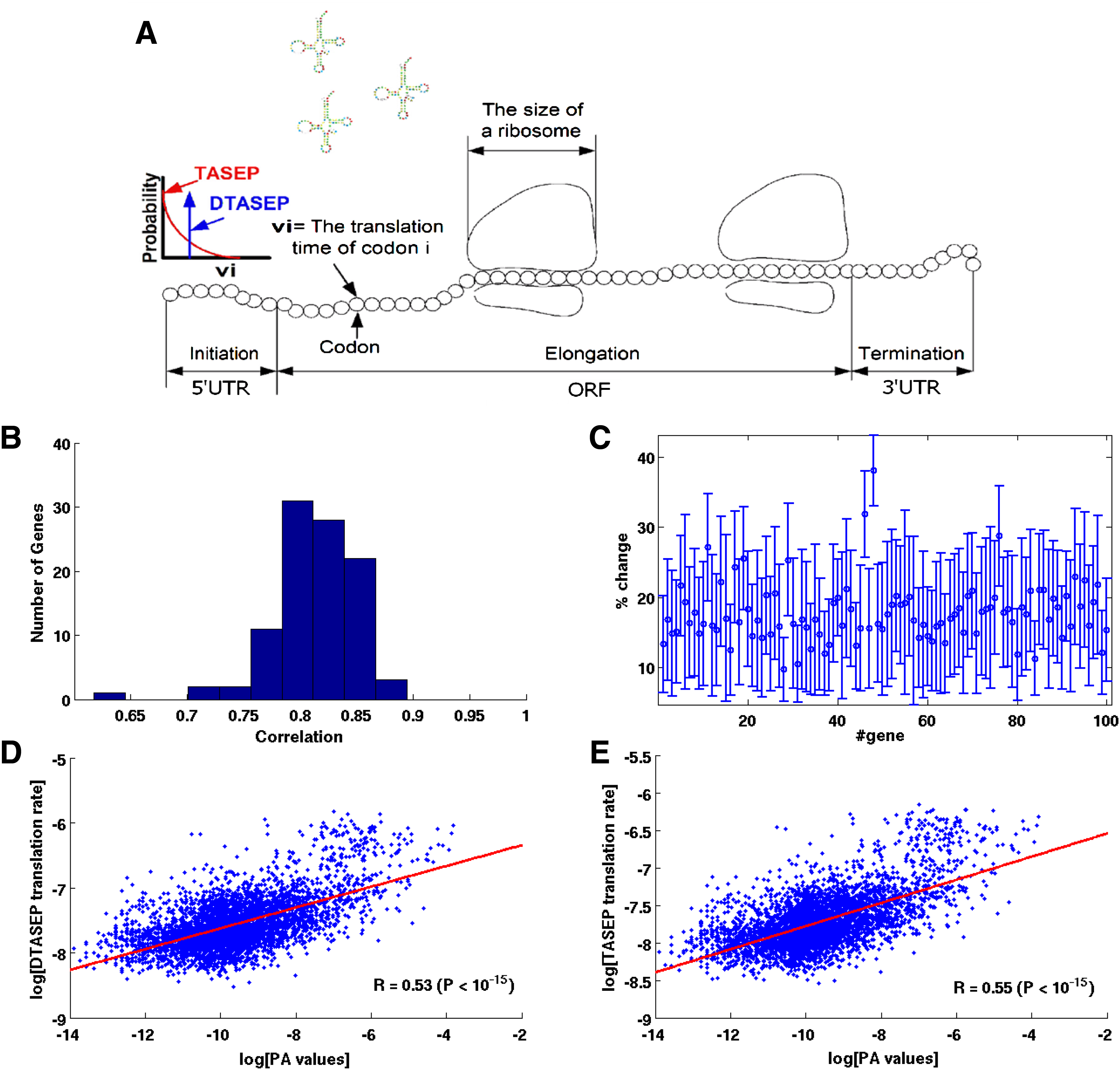
As a result, the Totally Asymmetric Simple Exclusion Process (TASEP) mathematical model used in previous studies (MacDonald et al. 1968; Heinrich and Rapoport, 1980; Shaw et al., 2003; Reuveni et al., 2011) was chosen for incorporating all these properties. A generic scheme of TASEP is presented in Figure 1A. In this model, ribosomes span over several codons and if two ribosomes are adjacent, the trailing one is delayed until the ribosome in front of it has proceeded onwards (Fig. 1A). Ribosomes were assumed to cover 11 codons (as the size of the footprint of the ribosome in eukaryotes (Ingolia et al., 2009); Tuller et al., 2010a; Reuveni et al., 2011) and initiation time as well as the time a ribosome spends translating each codon were defined as stochastic, similarly to these processes in nature. Specifically, in this study the initiation and translation times were defined to be exponentially distributed, but other distribution types could also be used. Average codon translation times were defined to be proportional to tRNA abundance in the host.
The models of translation.
Despite the rather simple description of the mathematical equation describing the flow of a single ribosome from one site (codon) to the next, no exact solution for the steady state translation rate exists for this model (Shaw et al., 2003). Because of TASEP's poor mathematical tractability, steady state ribosomal occupation and translation rate are calculated for this model using computer simulations.
However, to allow for analytical study of the translation process, we examined a deterministic model with similar properties, named Deterministic Totally Asymmetric Simple Exclusion Process (DTASEP) that has been employed in a few previous studies (Zhang et al., 1994; Tuller et al., 2010a). Thus, all analytical proofs of the various translation properties reported in this work were done on DTASEP. To show these properties' relevance to TASEP, these were also demonstrated using TASEP simulations.
Reuveni et al. (2011) suggested approximating TASEP with the deterministic Ribosome Flow Model (RFM). Therefore, several theorems reported in this article that are also correct for the RFM model were proved and appear in Appendix B together with a description of the RFM. In addition, in this study S. cerevisiae was used as a model organism to demonstrate some of the presented claims.
To supply justification of the selected mathematical models for describing the translation process, translation rates of all 5869 genes of the S. cerevisiae genome were calculated with TASEP and DTASEP. Spearman correlation between the calculated translation rates and the genes' Protein Abundance (PA) resulted in fair correlations (TASEP: R = 0.55, P < 10−15; DTASEP: R = 0.53, P < 10−15; Fig. 1D, E) suggesting that these models can be used for describing the translation process.
Recently it was suggested that the codon order of a gene can influence its translation efficiency (Cannarozzi et al., 2010; Kurt and Michael, 2010; Tuller et al., 2010b), therefore we compared the ability of both DTASEP and TASEP to grasp this effect in a similar manner. For this task 100 different S. cerevisiae genes with different PA were selected, and the codon order of each one of the genes was permutated for 1000 times. For each gene we computed the Spearman correlation coefficient between translation rates predictions of DTASEP and TASEP. The results show that, on average, the two models highly correlate (mean correlation: R = 0.81, P < 10−8; for more details, see Fig. 1B, C and Section 4.3). Further investigation also showed that DTASEP and TASEP models also achieve similar numerical values, with TASEP almost consistently resulting in lower rates (on average, translation rates calculated with DTASEP were higher by 17.75 ± 9.5% than when calculating with TASEP; Fig. 1C). Therefore, these results provide justification for the approximation of TASEP by DTASEP.
Throughout the paper several basic symbols are used, denoting key parameters of the DTASEP and TASEP models. To ease the reading continuum, these symbols are summarized as follows: let L denote the number of codons in a gene and let H denote the number of codons a ribosome covers. In this study we use the ∼ accent to mark random variables. Let Ui and
2.2. The influence of initiation time on translation rate
We start by studying the relation between initiation time and elongation rate. It was suggested before that either one of the initiation or elongation steps of the translation process can be rate limiting (Kudla et al., 2009; Tuller et al., 2010b; Reuveni et al., 2011; Plotkin and Kudla, 2010). In this article we formally show that for DTASEP, high initiation time values (relatively to the gene's codons translation time) have a major impact on translation rate. This property is formally stated in the following lemma:
Lemma 2
A high initiation time
The full proof of Lemma 2 based on the DTASEP model appears in section 4.4. To demonstrate this claim, translation rates of 100 different genes from S. cerevisiae genome were calculated using different initiation times, ranging from 1 to 15000 time units, while the host's codons translation times varied between 16.8 and 1355 time units. As seen in Figure 2A, for low initialization time values (1 time unit) the mean and standard deviation of the calculated translation rates are relatively high (4.9 × 10⁻⁴ ± 2 × 10⁻⁴), indicating that the translation rate of the genes is mainly dictated by the translation times of the codons composing the genes. For high initiation time values (10000 time units) the mean translation rates and their standard deviation decreased (to 9.28 × 10⁻⁵ ± 3.23 × 10⁻⁶), suggesting that translation rate is mainly dictated by the initiation time regardless of the genes' codon composition.
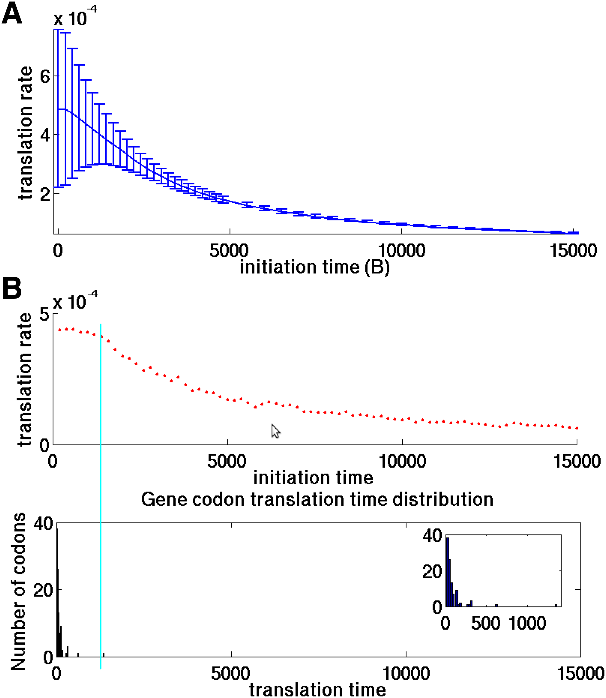
The effect of initiation time on translation rate.
This behavior was also demonstrated on a single gene (YJR011C). As seen in Figure 2B, translation rate remained almost constant for initiation values lower than the slowest codon in the gene (1355 time units). An increase in initiation time beyond this value caused to a decrease in translation rate and eventually entirely dictated it.
Thus, since we aimed at isolating the effect of codons (their composition and ordering) on translation rates, we neutralized the initiation time effect in Sections 2.3, 2.5, and 2.6 by setting the initiation time parameter to be lower than the translation time of the fastest codon in the genome (in practice, 65% of the fastest codon).
2.3. The influence of increasing translation time of a codon on translation rate
Intuitively, decreasing translation time of a codon in a gene should not decrease its translation rate. We formally phrase this claim into the following statement:
Lemma 3
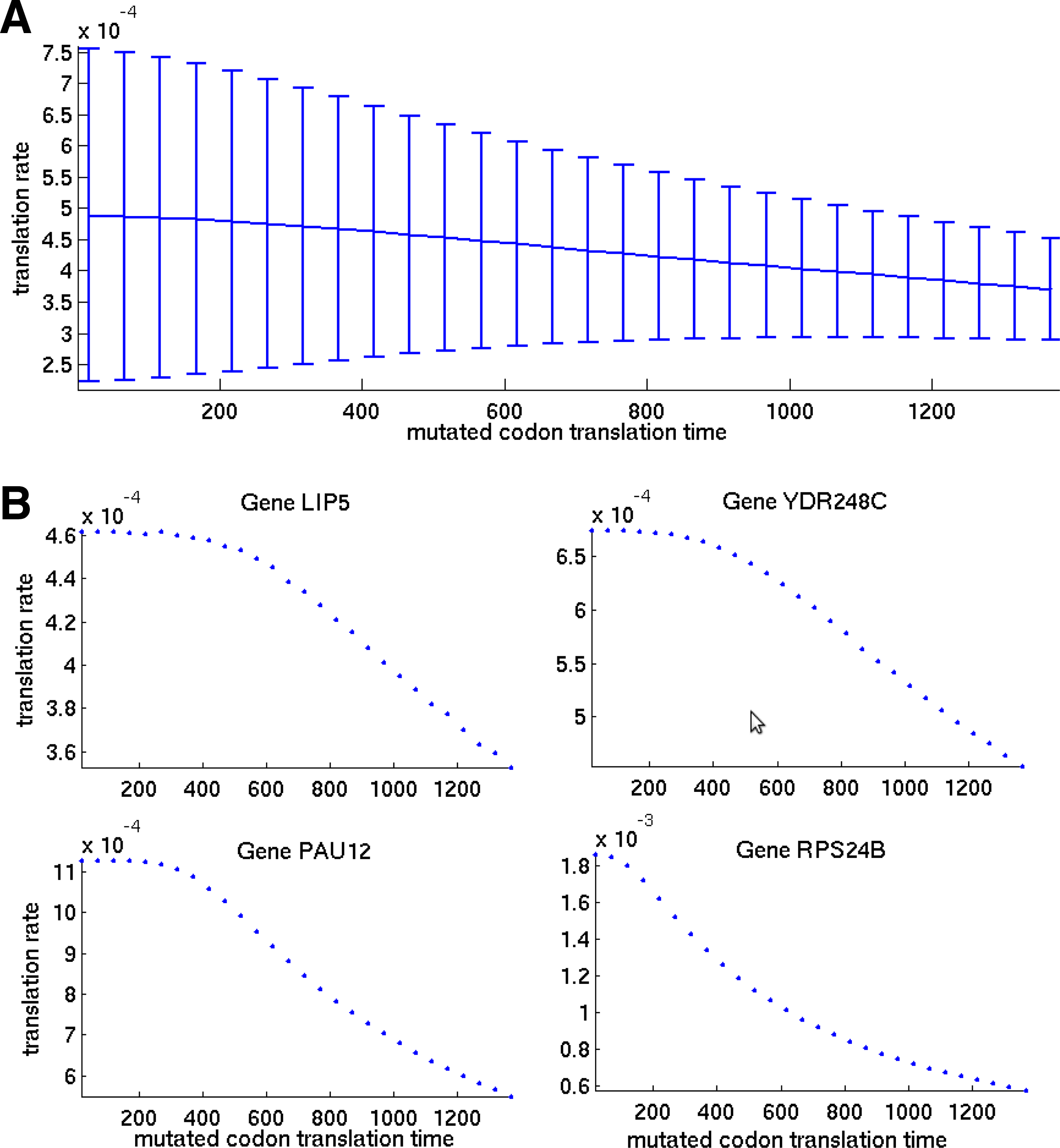
A decrease in one of the codon's translation time Ui cannot decrease the translation rate R of a gene.
The full proof of Lemma 3 appears in Section 4.4, and in this section it is also demonstrated on the same 100 genes selected for demonstrating Lemma 2 in Section 2.2. For each gene a random codon was selected and its translation time values were changed from 16.8 to 1400 with steps of 50 time units. Figure 3A presents the mean and standard deviation of the calculated translation rates for the selected genes as function of the translation time of the manipulated codon, while Figure 3B shows the translation rate values for four selected genes (LIP5, YDR248C, PAU12, and RPS24B). As seen from this simulation, high translation time values of even a single codon can drastically reduce the translation rate regardless of the genes' codon composition, while decreasing a codon's translation time can increase translation rate only up to a certain saturation value that is mainly dictated by translation times of other codons in the gene. This behavior was observed to be general, as demonstrated in Figure 3A.
Influence of translation time of a single codon on translation rate of a gene.
Therefore, adding a codon to the mRNA chain cannot increase translation rate, regardless of its value. This modification can be also perceived as increasing translation time of a codon from 0 to a finite value, which results in the inverse behavior described by Lemma 3. This observation was formalized in the following statement and its full proof appears in Section 4.4.
Lemma 4
Adding a codon to the mRNA cannot increase its translation rate R.
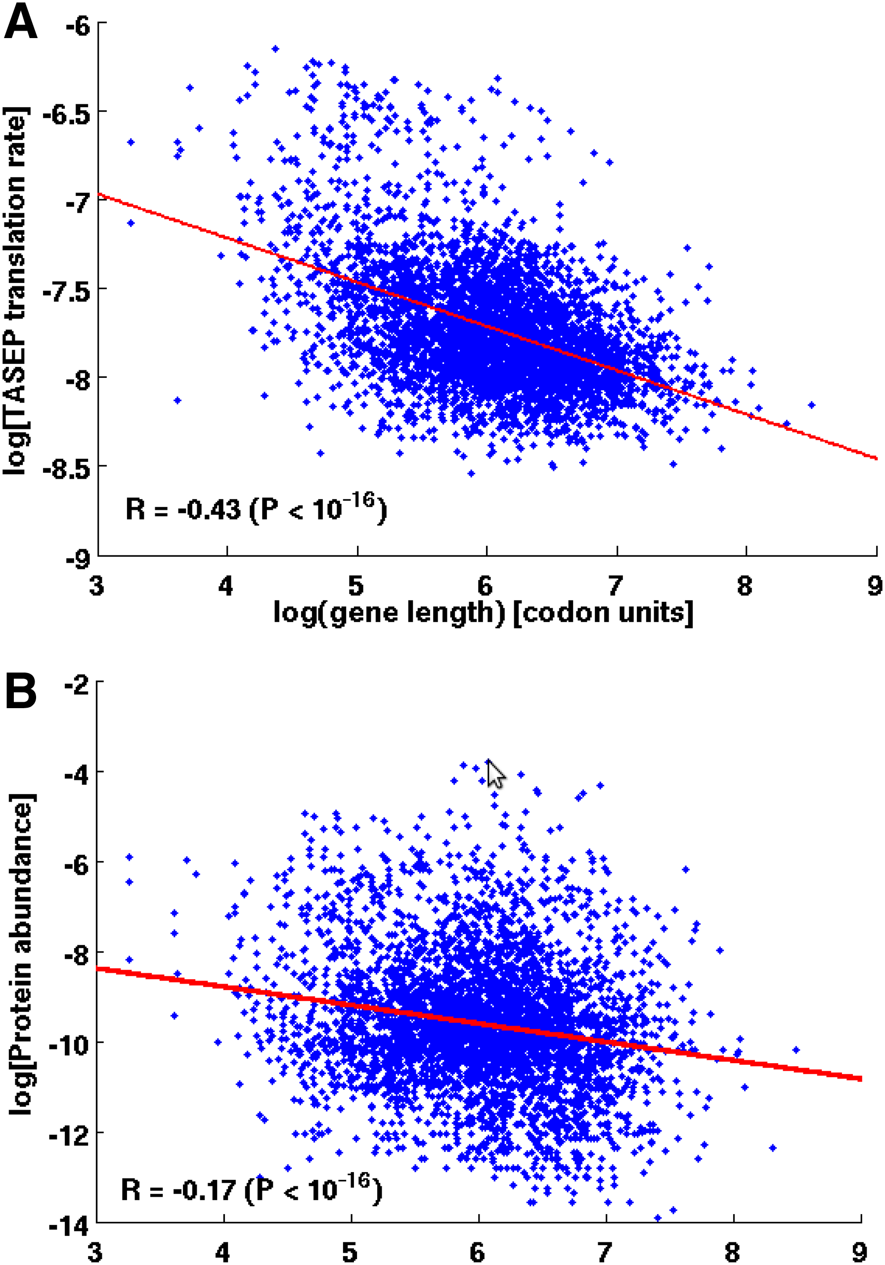
This lemma also suggests that for low initiation time values, where codon composition can be influential, longer genes have lower translation rates. This result partially supports the calculated negative correlation between the lengths of all genes in S. cerevisiae and their measured PA values (R = −0.17, P < 10−16; Fig. 4B). Spearman correlation coefficient between TASEP translation rate and gene length values were also found to negatively correlate (R = −0.43, P < 10−16; Fig. 4E) as suggested by the lemma.
2.4. Increasing translation rate of a codon(s) may have a negative effect on translation rate of a different gene in the host when the pool of ribosomes is finite
In the previous subsection it was shown that decreasing translation time of a codon in a gene cannot decrease its translation rate (Lemma 3). However, this modification may increase ribosomal density on the altered mRNA, and as a result may decrease the number of available free ribosomes in the cell. A steep decrease in the amount of available free ribosomes in the host can lead to ribosomal starvation and eventually reduce translation efficiency of other genes.
This effect was demonstrated using two different genes (SIF2 and RPL27B) taken from S. cerevisiae. First, we calculated the translation rates of two selected genes and the number or ribosomes allocated on each one of the mRNAs (for an infinite number of ribosomes in the pool). Next, we created a mutated fast version of one of the genes (SIF2) by reducing translation times of part of its codons and recalculated the translation rate and number of allocated ribosomes. The genes' codon translation times are described in Figure 5A, while the calculated translation rates and ribosomal densities are summarized in Table 1.
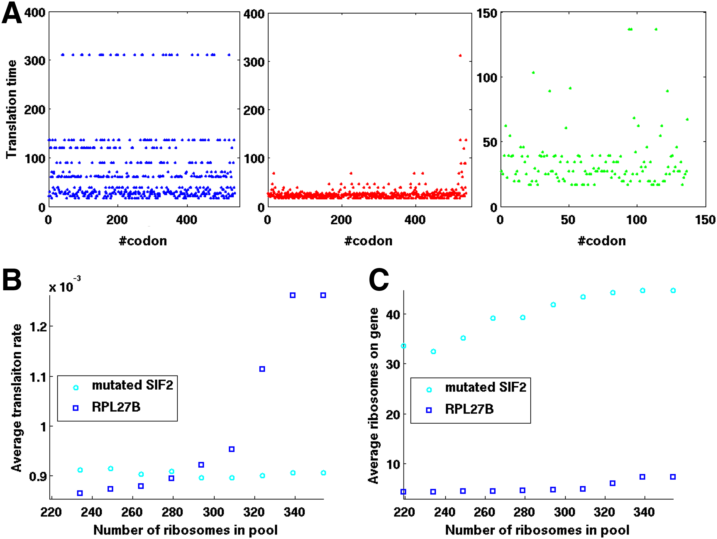
A simulation showing that improving the translation rate of some codons in a gene can decrease the translation rate of a different gene.
As can be seen from Table 1, for an infinite number of ribosomes in the pool, after reducing translation times of some of SIF2's codons, the translation rate of the gene increased by a factor of almost two, but also its ribosomal density.
In order to demonstrate the effect of this change in a host with a finite number of ribosomes, we simulated an environment of six mRNA copies for each one of the two genes (the mutated SIF2 and RPL27B). The simulation starts with a number of ribosomes that is equal to the needed number of ribosomes for each one the genes (before the mutation) multiplied by six. In the case of a finite number of ribosomes, we also assume that the initiation rate (initiation time−1) is proportional to the current number of available ribosomes in the pool, thus the initiation time of each one of the translated mRNAs was defined as:
where c is a normalization factor that was defined as the minimal translation time of codons in the host. Therefore we started with a pool that contains the number of ribosomes needed for translating the original SIF2 and RPL27B genes and in each step of the simulation we increased the number of ribosomes until reaching the needed number of ribosomes for the mutated SIF2 and RPL27B genes.
Figure 5B–C present the steady state translation rates and number of ribosomes on mutated SIF2 (cyan circles) and RPL27B (blue squares) for different number of ribosomes in the pool. As can be seen from the figures, translation rate of the mutated SIF2 gene did not change significantly for various amounts of free ribosomes in the pool (cyan circles) and was similar to the translation rate calculated for a pool of infinite number of ribosomes (Table 1). However, for a low number of ribosomes in the pool, translation rate of the RPL27B gene decreased significantly from 0.00138 to 0.00084 (blue squares). Increasing the number of ribosomes in the pool in the presence of the mutated SIF2 gene caused translation rate of the RPL27B gene to gradually increase until reaching a translation rate value similar to the one obtained for an infinite number of ribosomes (0.00132 vs. 0.00138).
For a low number of ribosomes in the pool, the average number of ribosomes per mRNA in the simulation decreased both for the mutated gene SIF2 and RPL27B gene (30.2 vs. 43.5) and (4.2 vs. 9.9) respectively, as can be seen in Figure 5B. This value also increased for both genes as the number of ribosomes in the pool increased, reaching similar values to those estimated with an unlimited number of ribosomes in the pool (45.49 vs.43.5 for mutated SIF2 gene and 8.23 vs. 9.9 for RPL27B gene).
Although ribosomal density of both genes was reduced for a low number of available ribosomes in the pool, translation rate of the mutated SIF2 gene did not decrease significantly. This could be explained by the specific features of the mutated gene: it was engineered with relatively efficient codons at its 5′ end, while codons at the 3′ end preserved their original relatively high translation time values. When a high number of ribosomes were available in the pool, they tended to accumulate on the 3′ end of the mutated gene, causing ribosomes to spend more time on its mRNA due to ribosomal “traffic jam.” Decreasing the number of available ribosomes up to a certain level (i.e., when no ribosome is delayed by other ribosomes) reduced the number of accumulated ribosomes on the mRNA without reducing translation time.
On the other hand, the ability of the mutated SIF2 gene to accumulate ribosomes reduced the number of free ribosomes in the pool, causing to a decrease in the ribosomal allocation of the RPL27B gene, that eventually led to ribosomal starvation and a decrease in its translation rate. When increasing the number of ribosomes in the pool, this value increased until reaching the translation rate value calculated for this gene when no restrictions were made on the number of available ribosomes.
It is important to note that the phenomenon reported in this section highly depends on the location of the altered codons and the magnitude of change in their translation time. Decreasing translation time of codons that do not eventually increase mRNA ribosomal density has no effect on the number of available ribosomes in the host, thus cannot affect in this manner the translation rate of other genes. This simulation aimed at demonstrating that increasing translation rate of a specific gene can reduce protein production rate of other genes, thus potentially interfering with the growth rate of the host. With this in mind, changing translation rate of a selected gene by using synonymous mutations should take into consideration changes in ribosomal allocation. In the next sections we show how to include this constraint in the design of genes with altered translation rates.
2.5. Attaining a low ribosomal allocation limit
As mentioned in the introduction, Tuller et al. (2010a) showed that on average the first 30–50 codons of a gene are translated with lower efficiency. In addition, in eukaryotes, the last ∼50 codons were observed to show higher translation efficiency. Inspired by this observation, we show in this section that given a gene with a finite set of codons, arranging the codons by monotonically decreasing translation times, reduces to a minimum the total time a ribosome is delayed by other ribosomes on the mRNA, thus achieves in steady state the lowest number of allocated ribosomes on the mRNA and the highest translation rate per ribosome. This phenomenon is formulated in Lemmas 5 and 6 and proved in Section 4.4. Thus, this observed trend in endogenous genes is mathematically optimal.
Lemma 5
Given a gene with a finite set of codons
Lemma 6
Given a gene with a finite set of codons
In such arrangement, no ribosome is delayed by other ribosomes on the mRNA, thus spends on each site only the time required for translating the relevant codon. Therefore the overall translation time a ribosome spends on the mRNA is minimized to a value dictated only by the translation efficiency of its codons.
This property was also demonstrated for the same 100 selected genes used in Sections 2.1, 2.2, and 2.3. For each one of the genes we performed 1000 random codon permutations and compared the number of ribosomes allocated on each permutation to the number of ribosomes obtained when ordering its codons according to their translation time in a monotonic decreasing order.
Figure 6A depicts for each gene the average, minimal and maximal steady state number of allocated ribosomes on the mRNA (using a vertical blue bar), and the number of allocated ribosomes for a monotonic decreasing arrangement (red square). The simulation results show that indeed the suggested arrangement of Lemma 5 attains minimal ribosomal allocation. A closer examination also showed that on average, monotonic decreasing arrangements induced only 22% of the mean number of ribosomes inferred for other gene permutations, thus suggesting that non-optimal genes in terms of ribosomal allocation can have a major influence on the host's resources.
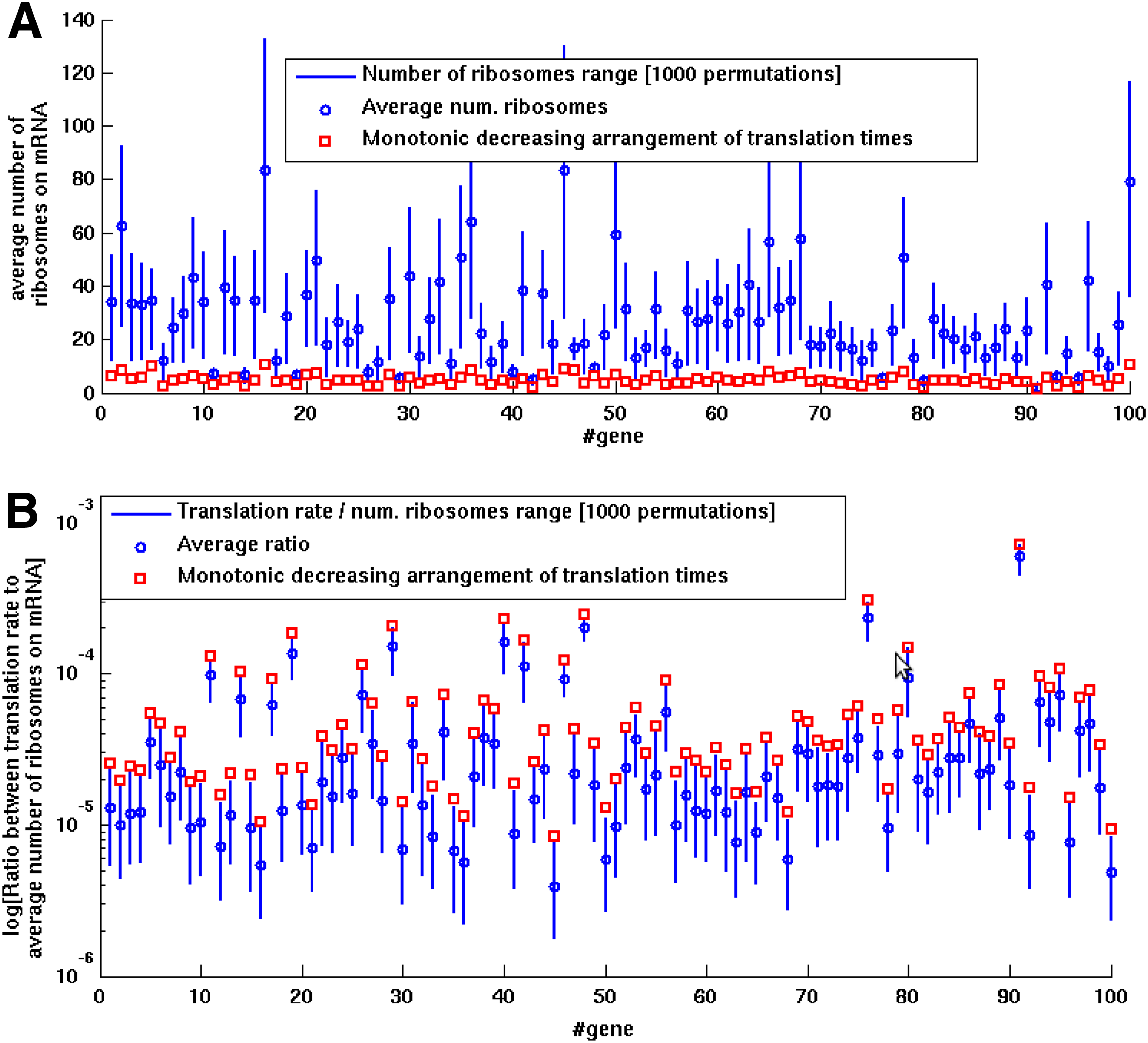
Codons permutation with monotonic decreasing codons translation times attains minimal number of ribosomes and maximal translation rate per ribosome in comparison to all other permutations. Analysis results of 100 S. cerevisiae genes calculated with the TASEP model. For each gene, the number of ribosomes on the mRNA
Moreover, as proved by Lemma 6, monotonic decreasing codon arrangement maximizes the ratio between translation rate to ribosomal allocation (see parameter K in Section 4.1). Figure 6B shows the range of this ratio for each one of the 100 genes (calculated for 1000 codon permutations) using a blue bar, and the achieved ratio using the monotonic arrangement, denoted with red squares. On average, this ratio was 80% higher for the monotonic arrangements in comparison the mean ratio inferred for other gene permutations. These results indicate that maximal translation rate per ribosome (i.e., minimal translation time needed for a ribosome to translate the mRNA) can be achieved by using a monotonic arrangement in terms of codon translation times.
2.6. A heuristic for controlling the translation efficiency of a gene while minimizing its ribosomal allocation
An efficient heuristic for designing heterologous genes with a specific translation rate and minimal ribosomal density was motivated by the optimality principle of Lemma 5.
Of course, in reality, the codons order of a gene cannot be changed without altering the coding of its amino acids, therefore the arrangement suggested by Lemma 5 is usually not possible. However, we can utilize this property by building different codon sequences using only synonymous mutations (that do not alter the gene's coding) with monotonically (or almost monotonically) decreasing codon translation times and search among them the sequence that has the closest translation rate to the requested value. Thus, the new engineered gene attains the requested rate, but with a minimal ribosomal allocation, which reduces the influence on other genes translation rate (as demonstrated in Section 2.4).
We name this heuristic Minimal Ribosomal density Target translation Rate (MRTR) heuristic. MRTR can be implemented with any model of translation that satisfies the Lemmas reported in this study (DTASEP, TASEP, or other similar model) and is based on two principles:
For simplicity, let us define the translation times of a sequence by using the translation time ranking of its codons. If the number of different possible translation times in an organism is P, we consider sequences of integers with values between 1 (lowest translation time) and P (highest translation time). Thus in general, a coding sequence of L codons induces PL possible sequences of translation ranks.
To find a series of codons with a specific translation rate and minimal ribosomal allocation coding a specific gene, binary search could be applied on only monotonic decreasing series (in terms of translation times) sorted by their translation rates.
It was already shown by Lemma 3 that translation rate of a gene could be increased by decreasing the translation time of one of the codons in the sequence, but a strict ranking of all possible codon combinations cannot be achieved straightforward only by using this principle alone. For example, given a sequence of three codons with P = 3 it is easy to determine by using Lemma 3 that the translation rate of series [3,3,3] is lower or equal to that of series [3,3,2], but the translation rate relation between series [3,3,1] and series [3,2,2] is not straightforward.
Therefore, a more systematic way is needed to sort all descending sequences according to their translation rate, to enable the application of a fast searching algorithm. Therefore, in this study translation rate of a monotonic decreasing series can be increased by decreasing the rank order of a single codon by a single rank unit in two ways:
1. Right Rule: decrease the rank order of the codon that already has the lowest rank that is not 1. In case several codons fulfill this condition, decrease the codon that is closest the 3’UTR. 2. Left Rule: decrease translation rank order of the codon with the highest rank. In case several codons fulfill this condition, decrease the codon that is closest the 3’UTR.
The suggested options were designed to preserve the series' monotonic decreasing characteristic. For example for P = 5 and L = 4 translation rate of a series with codons represented by ranks orders of [5,5,5,3] could be decreased by applying the Right Rule into [5,5,5,2] or by applying the Left Rule into [5,5,4,3].
Using these two rules, all descending series of L amino acids, each coded by P different codons, can be sorted according to their translation rate in a 2-D lattice. More details about the building of the lattice appear in 4.6.1. For example, Figure 9 shows all possible descending series for P = 4, L = 3. Each diagonal in the lattice contains a set of series that are ordered with respect to their translation rate, so that the series located at the top of a diagonal has the slowest translation rate and the series located at the bottom of a diagonal has the highest translation rate (with respect to all series in the diagonal).
To find a sequence with translation rate that is as close as possible to a specific wanted translation rate, a simple binary search could be applied on the translation rates of the series of each diagonal (Fig. 9). Let ɛ denote a certain threshold. Eventually candidate series from each diagonal that are in the limits of ± ɛ% distance from the original wanted translation rate value are re-evaluated. If several series fit this criterion, then the series with the lowest ribosomal allocation can be chosen.
It is worth mentioning that this type of mapping does not assure the uniqueness of a series in the lattice, therefore search time could be further reduced by using the fact that a series has a lower or equal translation rate in comparison to its left and right child series and their descendants. Let us assume that for a given diagonal, the wanted translation rate is bounded by two series Sj, Sj+1, where Sj+1 is the child on Sj. Using the above property, all child series of the upper bound have higher or equal translation rate, therefore they can be excluded from further searching. An example of this optimization appears in Figure 11 using the lattice presented in Figure 10. Here, the search starts from the outer left diagonal and the upper and lower bound series are contoured with green boxes. Child series of the upper bound in other diagonals (having translation rates higher than the upper bound series) are covered with a gray grid, thus can be excluded from the search. This step can be applied again when defining the lower and upper bound in the next diagonal to further reduce the number of tested series in the lattice.
Overall, the search time complexity of MRTR including the optimization step is O(f (L)(log(PL))2) and its space complexity is O(PL), where O(f (L)) is the time complexity of calculating the translation rate of a series of L codons. For more details regarding complexity calculations, see Section 4.6.
Applying the MRTR heuristic on real data measurements
When applying the heuristic on real genes, codons coding an amino acid have less than P possible values and translation rates cannot be calculated on series of codons rank order. Therefore to get a ‘full’ lattice with real translation times, for each amino acid we simply mapped each of the P possible ranking values to the real translation times of the codons coding it. An example of this mapping could be seen in Figure 12, where the host has P = 10 different codon translation times, but the specific presented amino acid can be coded by only three codons, represented by three rank orders. Therefore, several rank orders for this amino acid are missing real translation time values. To overcome this, the missing values were mapped to the closest lower rank order (and codon) that has an existing translation time. As a result, rank order series in the lattice that are selected for translation rate estimation by the binary search can be translated into series of real translation times that represent a possible codon combination (that does not alter the original gene coding).
It should be mentioned that other mapping variations could be implemented; for example, Grantham, (1974) showed that amino acids could be replaced by others with similar properties (thus increasing the number of possible translation times) or the heuristic could be applied on chunks of codons (Reuveni et al., 2011) (thus attaining P or higher different translation time values).
2.7. Demonstrating the MRTR heuristic on insulin gene
A common application in biotechnology focuses on producing human insulin from bacteria (Romanos et al., 1992; Abrahmsn et al., 1986; Moks et al., 1987). The human insulin gene depicted in Figure A1 was engineered using the MRTR heuristic, implemented with DTASEP, to achieve different translation rates (which are monotonically correlated to protein abundance) in S. cerevisiae, while consuming minimal ribosomal levels of the host.
First, a mutated version of the gene was engineered to achieve similar translation rates to the wild-type, but with a minimal ribosomal allocation (engineered gene 1). The resulting sequence is depicted in Figure A2. Second, another version of the gene was engineered to maximize translation rate without increasing ribosomal allocation of the original gene (engineered gene 2). The resulting sequence is depicted in Figure A3. Translation rates and ribosomal density were calculated for the original and both engineered genes also using TASEP. The results are summarized in Table 2. Additional details of the parameters used for calculating these values appear in Section 4.7.
As seen from the results, by using the suggested heuristic, translation rates could be preserved while reducing ribosomal usage by 60% (for both DTASEP and TASEP). On the other hand, translation rates could be increased by a factor of 3.84 for DTASEP and 4.25 for TASEP without increasing ribosomal allocation, thus allowing an increase in protein abundance without influencing the host. The wild-type and engineered gene sequences are presented in Figures A1, A2, and A3.
3. Discussion
In this study, we provided several new theorems related to the process of gene translation. In addition, we demonstrated how such theorems can be used for efficiently designing heuristics for engineering genes for heterologous gene expression.
This article emphasizes the differences between coding sequences that have been shaped by evolution and coding sequences that are optimized for various biotechnological goals. Sequences that are shaped by evolution are usually far from being optimal from the translation point of view (i.e., the models that were presented in the current study). This phenomenon can be explained by a few reasons:
First, the “optimization criteria” of evolution includes not only translation efficiency, but also additional considerations that influence the fitness of the organism. For example, the amino acid bias and the function/structure of the protein, the metabolic costs for generating the protein, the efficiency of the transcription stage, global considerations such as the effect of the translation of a single gene on other genes, and the response time—e.g., the time it takes to translate the first protein.
Second, often the evolution process does not converge to a global optimal point. For example, it is possible that all small mutations/changes in the organism's genome do not improve its fitness significantly; however, a large set of genomic changes (that cannot occur in a natural way) can improve it very significantly.
Third, organisms are evolving all the time as a response to environmental changes, resulting in constant change in the amino acids frequencies, the GC content of the genome, and cellular tRNA pool. Thus, to maintain the translation optimality of a coding sequence, the sequence should also keep evolving as a response to these changes, usually without converging to the optima point in terms of translation efficiency.
We practically demonstrated in this article how large-scale systems biology study of endogenous genes can be used for designing optimal coding sequences for biotechnological usage. In general, the approach demonstrated in this study includes the following steps:
1. Analyze endogenous genes with a required feature(s) (e.g., highly expressed genes, if the aim is maximizing translation rate or cost). Though, as discussed above, evolution does not perfectly optimize each coding sequence, thus on average, important/relevant features should be enriched in relevant groups of genes. 2. Formulate in an analytical/compact way the features that are over-represented in the gene set (e.g., highly expressed genes have relatively slower codons in the beginning of the ORF). 3. Formulate and prove mathematic theorem(s) explaining these features from a physical point of view (e.g., monotonically increasing profiles of translation efficiency optimize/minimize ribosomal density). 4. Use these theorem(s) for developing procedures for optimizing coding sequences (e.g., the MRTR heuristic).
One of the central results presented in this study is related to the effect of the order of codons on the number of ribosomes on the mRNA sequence. Our study emphasizes the need to minimize the ribosomal density in heterologous genes: genes with strong promoters but with non-optimal codons tend to consume a large number of ribosomes and cause a depletion in cellular resources, such as the number of available ribosomes and can decrease protein abundance of other genes. It is important to highlight the fact that slower codons at the beginning of a coding sequence lower its ribosomal density, even for cases when the number of ribosomes on the mRNA is relatively low and there are almost no collisions between ribosomes. This is done by effectively increasing the initiation time of ribosomes, such that the portion of the time that the gene is occupied by a ribosome(s) is lower.
In this study, we focused on the simplest models that capture the effect of codon order on translation efficiency. We supplied a few central lemmas about DTASEP, after showing that it supplies a fair and fast approximation of the TASEP model. These models can be generalized in various ways: for example, one can challenge the steady state assumption, consider other features of the coding sequence that may contribute to the translation rate of a codon (Tuller et al., 2010b, 2011), the effect of number of available ribosomes on the initiation rate, and the recycling of tRNA molecules (Cannarozzi et al., 2010). We aim to analytically analyze such models in the future in a similar way to the one presented here.
In addition, we aim to develop algorithms for optimizing coding sequences while considering additional features of the coding sequences such as the 5′UTR and 3′UTR of the gene (that may affect the initiation and termination rates) and the GC content of the gene that may affect the stability of its mRNA (Gu et al., 2010; Raab et al., 2010). This will increase the accuracy of the used theoretical models to enable synthesis of various genes with different translation rates that could be biologically validated in the near future.
4. Methods and Proofs
4.1. Modeling translation with DTASEP
Zhang et al. (1994) described the translation process using a deterministic set of equations; we name this model Deterministic TASEP (DTASEP). The mRNA was described as a 1-D lattice of L sites, L depicting the number of codons. Ribosomes were described by particles covering H consecutive sites at a time. A site can be covered only by a single ribosome at a time and ribosomes can translate a single codon at a time. A ribosome of length H can translate codon i if all i . . i + H − 1 sites on the lattice are free of other ribosomes. Initiation time describes the amount of time it takes a ribosome to bind itself to the mRNA chain, once the initiation site is available. Let us denote the initiation time by B(t) where t represents time. This value depends on several features, such as the number of free ribosomes and folding energy (Kozak, 1987; Alberts et al., 2002; Plotkin and Kudla, 2010; Gingold and Pilpel, 2011).
A ribosome can start binding to the mRNA if the initiation site is available and the first H codons are not occupied. Let us denote the time it takes a ribosome to translate codon i by Ui(t). In this study translation times were assumed to be constant, i.e., B(t) = B, Ui(t) = Ui. The model iteratively simulates attachment of ribosomes to the lattice and their advance on it according to the supplied parameters. Two important features are calculated in steady state: translation rate and the amount of ribosomes on the lattice. The following parameters were used in the model Zhang's model:
• n: index number of the ribosome participating in the translation simulation • N: steady state index number, defined as the state where the number of ribosomes on the message has reached a constant value • L: the number of sites in the lattice (i.e. the number of codons in the mRNA sequence) • H: the size of the ribosome in terms of number of codon sites; also used to define the minimum space (in codon units/sites) between adjacent ribosomes on the lattice • Bn: the time it takes for the n-th ribosome to form an initiation complex given that the initiation site is available. In this study it is assumed that Bn = B • Qn: the needed time for the ribosome to be released from the lattice after it reaches the stop (end) codon. In this study it is assumed that Qn = 0 • Un,i: the ‘nominal time’ required for the n-th ribosome to translate the i-th codon if no other ribosome ahead is blocking it to move forward. In this work we assumed Un,i = Ui • En,i: the ‘actual time’ it takes the n-th ribosome to translate the i-th codon. This value depends on Ui and on the delay caused by other ribosomes down the lattice, therefore En,i ≥ Un. By definition En,0 = B and En,L+1 = Q = 0. For simplicity let us mark EN,i = Ei • Tn,p: the total time it takes the n-th ribosome to finish translating the p-th codon and move forward to the next site, starting from the time the initiation site becomes available for binding. Therefore,
Notice that Tn,p = 0 for p < 0 or n < 1. For simplicity, let us mark TN,p = Tp. • In: the time the n-th ribosome has to wait until the binding site becomes available and the first H codons to be free of other ribosomes. This time is composed from the time it takes the n − 1-th ribosome to form an initiation complex and from the time it takes it to translate the first H codons. Therefore
For simplicity, let us mark IN = I; therefore, at steady state we get that
• Wn,i: the time delay of the n-th ribosome on the i-th site. This value is determined by the state of both the current ribosome n and the downstream ribosome n − 1. The delay of the n-th ribosome at site i is defined as the time the n-th ribosome has to wait after finishing translating codon i until the n − 1-th ribosome finishes translating codon i + H, so that the n-th ribosome will be able to move to the next site. Let us define t1 = 0 as the time that the n − 1-th ribosome can bind to the mRNA and t2 = In−1 as the time the n − 1-th ribosome moves to the H + 1 codon allowing the n ribosome to start binding to the mRNA. At time t3 = In−1 + Tn,i−1 + Un,i the n-th ribosome finishes translating the i-th codon and can be delayed at site i only if the n − 1-th ribosome did not finish translating codon i + H. The overall time it takes the n − 1-th ribosome to finish translating the first n + H codons and move to site i + H + 1 is defined by Tn−1,i+H. Let us define this time as t4. This of course is also the time the n-th ribosome moves to site i + 1. The overall time it takes the n-th ribosome to translate the first i codons and move to the next site is therefore
where Wn,i is the delay of ribosome n at site i caused by the the n − 1-th ribosome. Using both definitions of t4 we get that
following the next mathematical relationship:
Therefore, the actual time the n-th ribosome spends at site i is:
Negative Wn,i has no physical meaning, therefore is set to zero. Also, for i within the H last sites on the lattice, Wn,i also takes the value of 0, since when a ribosome reaches a site i such that i > L − H and finishes translating its codon, it already covers the next H sites down the lattice, therefore no other ribosome can delay it, resulting in
For simplicity let us mark WN,i = Wi. • Pn: the translation time of the mRNA by the n-th ribosome, which can be expressed as:
For simplicity let us mark PN = P. • D: the number of ribosomes per message at steady state. Defined as the number of initiations occurring in the period of time it takes a single ribosome to translate the mRNA in steady state. Therefore D is determined by the following relationship:
• Rn: the release rate of a ribosome from the message. Also referred as translation rate. This value is defined as {the time interval between the n-th and (n − 1)-th ribosome release}−1, which is mathematically expresses as:
In steady state Pn = Pn−1 = PN = P and In−1 = I, therefore the steady state translation rate is:
For simplicity, let us mark RN = R. • K: the steady state translation rate per ribosome measure, defined as the steady state translation rate divided by the number of ribosomes on the lattice in steady state
4.2. Modeling translation with TASEP model
Translation was also modeled using TASEP, as previously described by different studies (MacDonald et al., 1968; Shaw et al., 2003; Reuveni et al., 2011). Similarly to DTASEP, the mRNA is characterized by L sites. Each ribosome on the chain covers H codons and any codon may be covered by a single ribosome at most.
In each step of the simulation, a single ribosome can attach itself to the lattice or advance on it if the first/next
Thus, the time between events (initiation/jump) is exponentially distributed with rate
The steady state translation rate was determined by counting the total ribosomes that finished translating the mRNA during the simulation divided by the total simulation time. In this study 1,000,000 steps were used for achieving an initial scattering of ribosomes on the mRNA and another 100,000,000 steps for calculating the translation rate.
The number of needed iterations for achieving steady state solution highly depends on the values of L, H, B and
4.3. Showing correlation between DTASEP and TASEP models
In the absence of direct measurements of translation rates, protein abundance (PA) was selected as a predictive measure, assuming that PA of a gene is expected to increase monotonically with translation rate (Reuveni et al., 2011).
In this study characteristics of the translation models were demonstrated on genes taken from S. cerevisiae genome, unless stated otherwise. Codon translation times were taken from Tuller et al. (2010a).
To estimate the degree of similarity between translation rates calculated with DTASEP and TASEP in respect to the effect of codon ordering on translation, 100 random genes with different translation rates were selected from the S. cerevisiae genome and for each gene codon locations were permutated 1000 times. Translation rate was calculated for each permutation using the mathematical models. Spearman correlation coefficient between TASEP and DTASEP translation rates was calculated for each gene apart (for all its 1000 permutations). The results of this validation are presented in Section 2.1 and in Figure 1B,C.
4.4. Characteristics of DTASEP translation model
Lemma 1
In steady state, if a ribosome that finished translating the i-th codon is being delayed by other ribosomes down the lattice, the following relationship exits:
otherwise
Proof
By definition, in steady state the delay of the ribosome at site i is determined by the following relationship:
By definition
therefore
thus
For W
i
=0, using the definition of Wi and eq. (15) we get that
therefore
Lemma 2
A high initiation time
Proof
The steady state translation rate is defined as R = I−1. By definition, we get that
The delay Wj of the last H codons is zero. Let us mark by m the biggest index with Wm > 0. Therefore by using Lemma 1, I can be expressed only by
However, the I variable from eq. (20) is at least of order of O(B), while the variable I from eq. (21) is of order of
indicating that
Lemma 3
A decrease in one of the codon's translation time Ui cannot decrease the translation rate R of a gene.
Proof
Let us select a general codon i and mark the decrease in its translation time by ΔUi, so that the codon's new translation time will be
Let us mark the rest of the codons translation time after this change with
First, let us define m as the biggest index of the site with Wm > 0, s.t. Wm+k = 0, ∀k > 0. Let us mark using
Using the above definition, let us check the relation between I and 1. m = 0 2. 3. 4. 5. 6.
resulting in:
1. Given m = 0 and If i ≤ H then If i > H then If m = 0 and therefore 2. For resulting in 3. For 4. For resulting in 5. For resulting in 6. For where Wj are the possible delays at sites resulting again in We have shown that for all possible values of m,
Lemma 4
Adding a codon to the mRNA cannot increase its translation rate R.
Proof
As mentioned in the definition section, R = I−1. Let us assume that R is the steady state translation rate of a mRNA with L codons. Now, let us assume that we decrease the translation time of one of the codons i from Ui by by Ui, such that Ui = 0. The reduction of the translation time of a codon to 0 is equivalent to removing it from the sequence, thus obtaining a new sequence with L − 1 codons. Let us mark the translation rate of the new sequence with
Therefore, the translation rate R of a sequence with L codons cannot be higher than the translation rate of its partial series (preserving the same codon order) with a lower number of codons. ▪
Lemma 5
Given a gene with a finite set of codons
Proof
Let us assume that for such codon arrangement a ribosome at steady state can be delayed at some sites. Let us define by m the biggest codon index such as Wm > 0. Using Lemma 1, for such site the following relationship exists:
However, by definition
Because of the selected arrangement (Ui ≥ Ui+1), we get that
therefore by combining eqs. (33), (34), and (35), we get that
therefore, such site m with Wm > 0 cannot exist, resulting in W j = 0, ∀j.
In DTASEP, the number of ribosomes on the lattice at steady state, D, is defined as
which can be also expressed as
To minimize the number of ribosomes D on the mRNA we need to minimize the numerator while maximizing the denominator of eq. (38):
For a monotonic decreasing series (Ui ≥ Ui+1), we get that the nominator
We will show that no other codons arrangement can achieve a lower D value than achieved with a monotonic decreasing series.
First, let us mark with I* the total initiation time of a monotonic decreasing series, having the slowest H codons located in the first H sites. Let us mark those codons with
For a general (non-monotonic decreasing) series, let us mark again with m the biggest codon index such that Wm > 0. If such m exists, then by using Lemma 1, we get that
Because of the non-monotonic arrangement we get that
If such m does not exist, then I is defined only from the translation time of the first H codons, which again result in I ≤ I*.
It was already shown that for a general H, a monotonic decreasing series has Wj = 0, therefore such arrangement minimizes the nominator
Lemma 6
Given a gene with a finite set of codons
Proof
By definition, the steady state translation rate per ribosome measure K is mathematically defined as
Thus, in order to maximize K, P should be minimized. Using the definition of P, we get that
It was already shown in Lemma 5 that a monotonically decreasing series has Wi = 0, thus minimizes P and maximizes K. ▪
4.5. Used data
Various properties of the used translation models in this paper were demonstrated on genes taken from the S. cerevisiae genome. Codon translation times were taken from Tuller et al. (2010a). The insulin gene sequence was taken from the National Center for Biotechnology Information.
4.6. MRTR heuristic for determining translation rate using synonymous mutations—additional details
4.6.1. Ordering all descending series according to their translation rate
As mentioned in Section 2.6, in order to find a sequence with a specific translation rate and minimal ribosomal allocation, we can apply a binary search algorithm on all descending sequences (according to their codon translation times) sorted by their translation rate. As already shown in Section 2.6, the sorting of all descending series is not trivial due to the multiple possibilities of increasing translation rate of a series only by decreasing translation time of a single codon.
The P possible codon translation times of a host can be described also according to their rank order Wi. Therefore Wi = 1 represents the lowest translation time while Wi = P represents the highest translation time in the host. In this study, we used two methods for increasing translation rate of a series:
1. Right Rule: decrease the rank order of the codon that already has the lowest rank that is not 1. In case several codons fulfill this condition, decrease the codon that is closest the 3’UTR. 2. Left Rule: decrease translation rank order of the codon with the highest rank. In case several codons fulfill this condition, decrease the codon that is closest the 3’UTR.
For specific implementation of these two rules, see also the pseudo code in Figures 7 and 8.
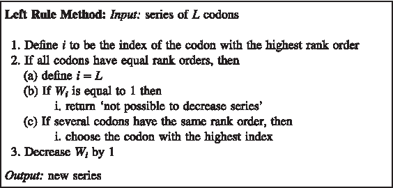
Left Rule pseudo code.
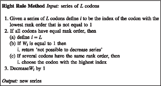
Right Rule pseudo code.
Therefore all descending series representing a gene with L codons and P possible codon translation times in a host can be mapped and sorted in a lattice according to their translation rate in the following manner:
1. Start with the series containing the codons with the highest possible rank order (the series with lowest translation rate), i.e., 2. Apply Right Rule on the current sequence and reapply it recursively until reaching the series with the fastest possible translation rate, i.e. 3. For each sequence in the outer left diagonal, apply the Left Rule and reapply it recursively until reaching the series with the fastest possible translation rate, i.e.,
An example of this building for L = 3 and P = 4 can be seen in Figure 10. Of course another lattice can be achieved by first building the outer left diagonal using the Left Rule and then by applying recursively on each one of the series the Right Rule, all left-to-right internal diagonals could be built. An example of this building for L = 3 and P = 4 can be seen in Figure 9. Although the two lattices contain the same series, they are mapped in a different order, therefore the lattices are not identical.
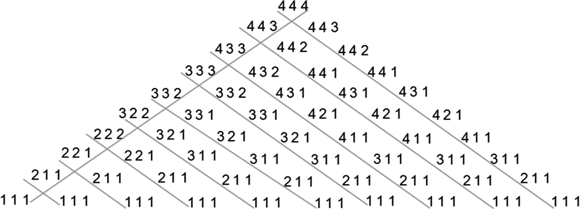
An example of the search lattice for L = 3 and P = 4. The external left diagonal is first built by applying the Left Rule recursively, starting with the series with the slowest translation rate (in this example [4 4 4]). Then, on each series in the outer left diagonal the Right Rule is applied recursively until translation rate could not be further increased (in this example [1 1 1]). Each child node in the lattice represents a series with higher or equal translation rate in comparison to its father's sequence.
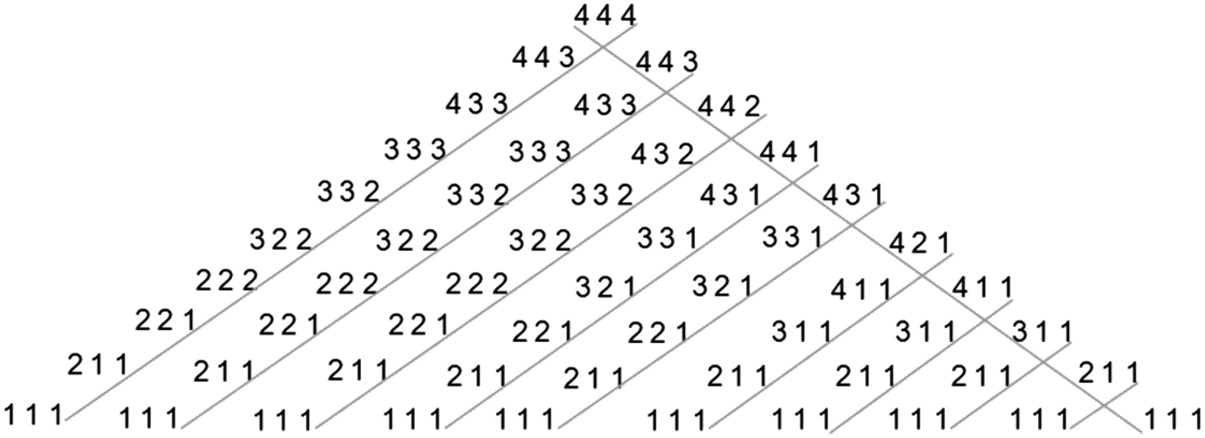
Another mapping of the lattice for L = 3 and P = 4. In this method the outer right diagonal is first built by applying the Right Rule recursively, and then, on each one of its series the Left Rule is applied. Each child node in the lattice represents a series with higher or equal translation rate in comparison to its father's sequence.
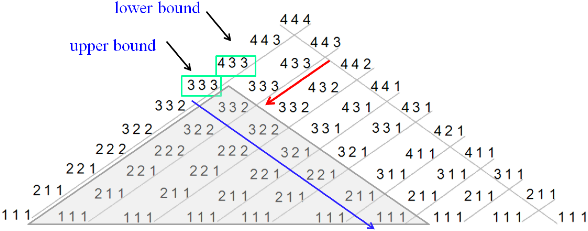
Optimizing search in the lattice. After searching the wanted translation rate in the external left diagonal, two sequences are found to upper and lower bound the wanted translation rate, depicted in this figure by green boxes. Given the upper bound, series below it in left diagonals (underlined by the blue arrow) and their child series have higher or equal translation rate to the upper bound, therefore can be excluded from the search (marked with the gray triangle). Thus the search in the next diagonal can be reduced, as depicted by the red arrow in this figure.
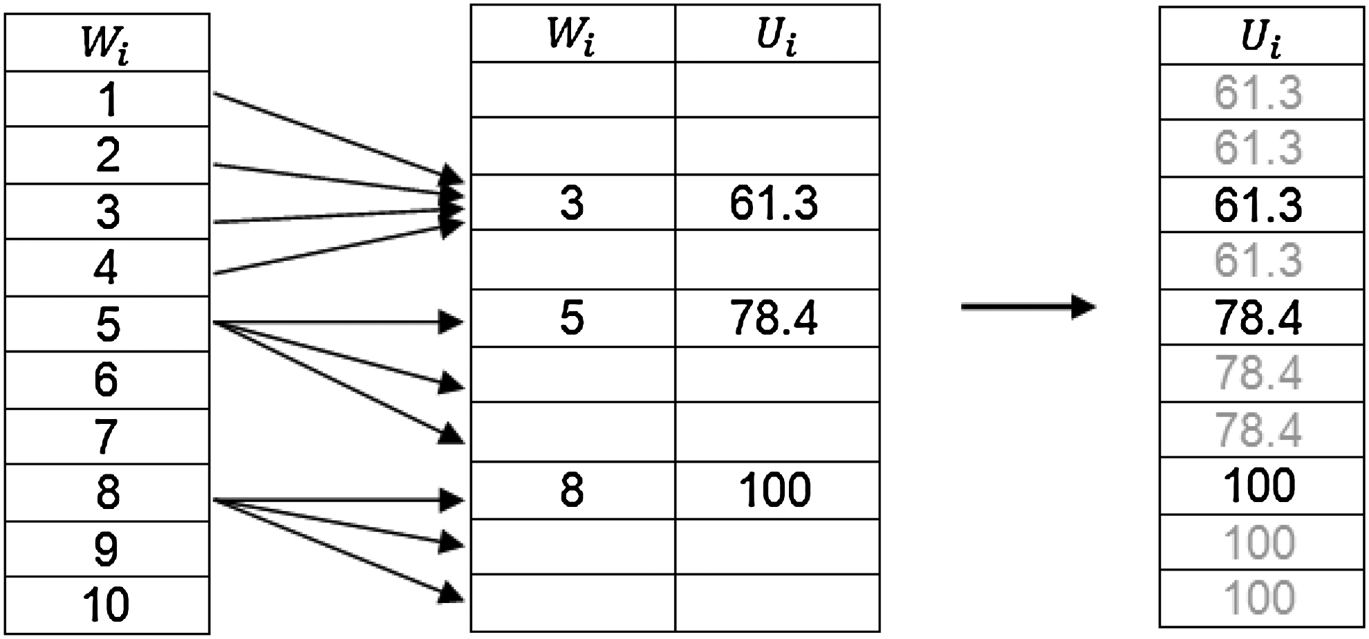
Mapping example between continuous ranking variable W i values to real (sparse) translation time values U i of codons coding the same amino acid. In this figure P=10. The left table depicts the possible values of the ranking variable (1-10) for this specific host. The middle table presents the mapping between ranking variables to codon translation times for a selected amino acid, where only three codons can code it. As a result, other ranking orders are missing a mapping to real translation times. To overcome this, ranking orders without a mapping are mapped to the closest lower possible translation rate, achieving a full mapping between the ranking variable and real translation times (without changing the coding of the amino acid), as depicted in the right table.
4.6.2. Time complexity analysis for building the lattice
The straightforward time complexity of Left Rule and Right Rule methods is O(L). This complexity can be further reduced to O(1) by copying the series from the previous node on the lattice and managing the indexes of the codons with the highest and lowest rankings. The external right and left diagonals of the lattice contain (P − 1) L + 1 nodes, therefore the total number of nodes in the lattice is
Thus, the time complexity of building the lattice is
4.6.3. Memory complexity analysis for building the lattice
As shown in the previous section, there are
4.6.4. Time complexity analysis for search heuristic
Given a set of N sorted numbers, the time complexity of a binary search is O (log (N)). The time complexity for calculating the translation rate given a sequence of L codons and a translation model is O(f (L)), therefore the time complexity of finding the closest possible rate on a diagonal of N sequences is O(log (N) f (L)). Given (P − 1)L + 1 internal diagonals of length N, the time complexity of finding the closest rate in each diagonal is therefore
However, the diagonals in the lattice are not equal, but of length 1. (P − 1)L + 1, reducing time complexity to
This of course it an upper bound for the search heuristic. Using the suggested optimization in Section 2.6, on average the length of each diagonal can be reduced by a factor of 2 (relatively to its previous diagonal), getting the following complexity:
Finally, to find the closest rate among all candidate rates (one series per internal diagonal) we need another ((P − 1)L + 1) comparisons, overall attaining a time complexity of
In general, O (f(L)) ≫ O (PL); therefore, the last factor can be removed, resulting in time complexity of
4.6.5. Time complexity analysis for mapping ranking series to real translation time series
A translation table between codon ranking order to real translation times could be built once for each amino acid type, with time complexity of O(P). Therefore, the mapping of each one of the rank orders of a series to its real translation time can be done in O(1). Each series contains L codons; therefore, the time complexity required to map between a ranking series to a translation time series is O(L). The mapping can be applied on a rank order series only when the binary search on each diagonal requests to know a series specific translation time. In the previous section, it was shown that the translation model is activated O((log(PL))2)) times; therefore the mapping time complexity is
4.6.6. General time and memory complexity analysis
The general time complexity is determined by building and searching on the lattice, resulting in
Given that O(f (L)) ≫ O(L2P2), the overall time complexity is
The memory complexity is determined by the dimension of the lattice, resulting in O(PL) space complexity.
4.6.7. Implementation optimizations
This MRTR heuristic can be implemented using DTASEP or TASEP models to calculate the translation rate of a given series. However, because DTASEP parameters are deterministic, less iterations (by a few orders) are needed to achieve steady state translation rate when compared to TASEP. To shorten running times, MRTR could be first implemented using DTASEP and then its results could be revalidated with TASEP.
4.7. Applying MRTR on insulin gene—technical details
The human insulin sequence was taken from for Biotechnology Information is depicted in Figure A1. Codon translation times were taken from Tuller et al. (2010a).
The genes in both demonstrations were engineered with MRTR, using the DTASEP model and also re-validated with TASEP. These models were run with the parameters appearing in Table 3.
4.8. DTASEP, TASEP, and MRTR running times—a short benchmark
DTASEP, TASEP, and MRTR running times were measured on a Quad Core working station with 4G memory and Ubuntu 11.04 operating file system. The code was implemented and run on Matlab 7.8, 32-bit.
For benchmarking purposes, DTASEP and TASEP were run 100 times on the insulin gene presented in Figure A1 to get an average running time of the models, using the parameters presented in Table 3. The MRTR running time was measured for generating both engineered genes. The results are presented in Table 4.
Appendix
Appendix A
Wild-type human insulin sequence.
Engineered insulin sequence achieving similar translation rate as the wild-type with minimal ribosomal allocation
Engineered insulin sequence achieving maximal translation rate with similar ribosomal allocation as the wild-type
Appendix B
Another deterministic model describing the translation process was suggested Reuveni et al. (2011). The mRNA strand was also described by a 1-D lattice of L sites and the ribosome length was set to the size of a single codon. To overcome this limitation, mRNA molecules were coarse grained into chunks of C sites. This parameter was associated to the ribosome's various geometrical properties and selected by maximizing the correlation between translation rates of this model to protein abundance. Given that the first site is not occupied, ribosome initiation rate was denoted by λ (which is equivalent to B−1 parameter in DTASEP). A ribosome occupying site i moves with a rate λ i to site i + 1, given that the later is not occupied by another ribosome (λ i is equal to U i −1, used in the DTASEP model). The translation process of this model is depicted by a set of differential equations, describing each the movement of a ribosome from site i to site i + 1. Their solution supplies the steady state occupation probabilities of each site and the ribosome flow through the system.
B.1. General model description
The following parameters were used to describe the RFM model:
• L - the number of sites (codons) in the translated mRNA • C - the number of sites in a chunk • λ - initiation rate, given that the first site is not occupied by another ribosome • λ
i
- the rate of a ribosome translating codon i, given that no ribosome occupies site i + 1 • pi(t) - the probability that site i is occupied by a ribosome at time t • π
i
- the steady state occupation probability of site i • R - the steady state ribosome flow through the system • D - number of ribosomes per message at steady state, defined as the sum of densities
• The flow rate of ribosomes into the system is equal to the initiation rate multiplied by the probability of the first site to be empty, i.e.
• The flow rate of ribosomes at site i is given by the flow entering site i from site i − 1 minus the flow exiting site i to site i + 1
• K - the steady state translation rate per ribosome measure is defined as
The ribosome flow model is described by the following set of differential equations:
The steady state solution of eq. (44) is:
where the steady state occupation probabilities
B.2. Correlation between RFM translation rates and PA
The RFM model uses ribosomes of single site length. To overcome this limitation, mRNA sites were coarse grained into chunks which their size was optimized by maximizing the correlation between PA of S. cerevisiae and its genes translation rates. Maximal Spearman correlation coefficient achieved a value of 0.67 (P values < 10−14), resulting in chunks of 23 sites, similarly to previous obtained results by Reuveni et al. (2011).
B.3. Correlation between RFM and TASEP translation rates
To establish similarity between RFM and TASEP models, translation rates were calculated for 1000 codon location permutations for different 100 genes from S. cerevisiae genome. Average Spearman correlation coefficient between TASEP and RFM translation rates was 0.89 (P < 10−8).
B.4. Characteristics of the RFM model
Lemma 2
A low initiation rate
Proof
This proof is taken Reuveni et al. (2011).
As seen from eq. (45), the steady state translation rate R is determined by
Thus for low initiation rates we get that
Lemma 3
A positive change to one of the λ i -s increases the protein production R.
Proof
Let us negatively assume that a positive change in one of the λ i s decreases R.
A general change of Δλ to λi,1 < i < L will change the steady state solution of eq. (45) to:
After extracting eq. (45) from eq. (48) we get that:
All rates{λ
i
} and occupation probabilities{π
i
}are positive by definition, therefore if ΔR < 0, from eq. (49) we get that
resulting in Δπ L < 0.
Using ΔπL < 0, we can determine ΔR for i = L − 1, with the help of eq. (49), getting
If ΔR < 0 then
therefore
But
1. λL−1 > 0 2. (1 − π
L
− ΔπL) > 0 3. πL−1 >; 0 4. Δπ
L
< 0
therefore it can be derived from eq. (52) that
When assuming ΔR < 0 we can show in the same manner that
By checking eq. (45) for a general i we get that
Using the assumption ΔR < 0 we get from eq. (55) that
Again, this equation can be rewritten as
By using λ
i
> 0, 0 < π
i
< 1, Δπi+1 < 0 on the last inequality we get that
For 0 < π
i
< 1, Δπi+1 < 0 the right factor holds (1 − πi+1 − Δπi+1) > 0, therefore we can reduce the last inequality to
However, Δλπ i ≥ 0, (λ i + Δλ) > 0 therefore we conclude that Δπ i < 0.
Using this, we can show that for a change Δλ to λ
i
, 1 ≤ i < L, if Δ R < 0 then
When the change Δλ > 0 is applied to λ
L
, we get from eq. (49) that
By checking equation
under the assumption that ΔR < 0 we get that
By definition λ
L
> 0, Δλ > 0, π
L
> 0, therefore Δπ
L
< 0. Using this, we similarly can show that for a change Δλ > 0 applied to λ
L
, the assumption ΔR < 0 derives
Therefore we showed that for any positive increase Δλ > 0 to any λ j , 1 ≤ j ≤ L, causes a decrease in protein production rate ΔR < 0, the occupation probabilities will also decrease, i.e.{Δπ j } < 0.
However, by definition (see eq. (49))
For ΔR < 0 we showed that Δπ1 < 0. Again, by definition λ > 0, therefore
contradicting our assumption.
Therefore, we conclude that for any positive increase Δλ > 0, in any of the λ j , 1 ≤ j ≤ L, ΔR cannot decrease.
Let us show that for Δλ > 0, the solution of eq. (45) must change. Let us define
and let us define
Let us denote the solution of eq. (45) given
Claim
For the defined
Proof
Let us assume
therefore the production rate R is identical in both cases. This means that the jth equation in the equation set (45) fulfills
Because
contradicting the made assumption.
In the same manner we can also contradict the assumption when
or
Because {Δπ j } is the steady state solution for eq. (45), for Δλ > 0 the occupation probabilities{Δπ j } have to change, therefore any positive increase Δλ > 0 will positively increase the protein production rate R. ▪
Lemma 4
Adding a new codon the mRNA in the RFM model decreases the translation rate R.
Proof
See proof for DTASEP model.
B.5. The correctness of Lemma 5 and Lemma 6 for RFM
Using DTASEP, it was proven that given a gene with a finite set of codons
This claim seems to be correct for most codon permutations when validated with various simulations on the RFM model. However, some scenarios were found not to obey this rule. For example for λ = 10 and
as shown also by Reuveni et al. (2011).
This equation can be rewritten as as a cubic equation
and analytically solved, supporting the presented findings.
Another example contradicting Lemma 6 was found for λ = 10 and
Footnotes
Acknowledgments
We would like to thank Elchanan Mossel for helpful discussions. T.T. was partially supported by a Koshland fellowship at Weizmann Institute of Science.
Disclosure Statement
No competing financial interests exist.