A Linearized Constraint-Based Approach for Modeling Signaling Networks

Abstract

With the unparalleled increase in the availability of biological data over the last couple of decades, accurate and computable models are becoming increasingly important for unraveling complex biological phenomena. Past efforts to model signaling networks have utilized various computational methods, including Boolean and constraint-based modeling (CBM) approaches. These approaches are based on solving mixed integer linear programs; hence, they may not scale up for the analysis of large networks and are not amenable for applications based on sampling the full spectrum of the solution space. Here we propose a new CBM approach that is fully linear and does not involve integer variables, thereby overcoming the aforementioned limitations. We describe a novel optimization procedure for model construction and demonstrate the utility of our approach on a reconstructed model of the human epidermal growth factor receptor (EGFR) pathway, spanning 322 species and 211 connections. We compare our model's predictions to experimental phosphorylation data and to the predictions inferred via an additional Boolean-based EGFR signaling model. Our results show high prediction accuracy (75%) and high similarity to the Boolean model. Considering the marked computational advantages in terms of scalability and sampling utilization obtained by having a linear mode, these results demonstrate the potential promise of this framework for the study of cellular signaling.

1. Introduction

Working models of cellular signaling are a key to understanding information processing and regulation in cells. On the topological level, many pathways have been mapped in detail and are deposited in large-scale databases such as Kyoto Encyclopedia of Genes and Genomes (KEGG) (Kanehisa and Goto, 2000). However, our understanding of their underlying logic and workings is still in its infancy.

Kinetic models based on differential equations are the current gold standard for modeling network events such as signaling, but as they are practical only in small-scale cases and require knowledge of many hard-to-assess parameters, mid- to large-scale signaling models mainly focus on static rather than dynamic descriptions. Such static models include Petri nets (Steggles et al., 2007) and Boolean (logic) networks (Li et al., 2009; Saez-Rodriguez et al., 2009). Recently, it has been suggested that the CBM approach could be adopted for exploring the properties of cellular signaling networks (Hyduke and Palsson, 2010). Until now, the vast majority of CBM studies in biology have focused on (i) generating genome scale metabolic models for various organisms; and (ii) developing analytical tools to use these models to learn about metabolism, with high level of prediction accuracy for variety of networks responses and phenotypes (Price et al., 2004a).

CBM models have been used in the past to describe signaling networks, mainly employing topological methods of extreme pathways analysis to elucidate central modes of signaling in the networks studied (Papin and Palsson, 2004a,b). A recent study also indicated that the CBM framework can help elucidating combinations of inputs that will create a desirable phenotype or intervention strategies that can help prevent undesirable phenotypes (Dasika et al., 2006).

Here we take this computational framework one step forward. Previous signaling CBM studies included a combination of linear programming (LP) and the use of integer variables. The CBM integer variable formulations are NP-hard and one of the Karp's 21 NP-complete problems (Karp et al., 1974), and therefore they have the significant disadvantage of becoming computationally intractable when applied to large and multivariate systems. Furthermore, due to the non-convexity of mixed integer systems, uniform sampling of the entire solution space to provide an unbiased assessment of reaction network states is impossible (Price et al., 2004a,b). Recently, a signaling CBM model of the human Toll-like receptor system, including 909 reactions that link 752 chemical species, was published (Li et al., 2009). Although this comprehensive, manually corrected model is purely linear, it doesn't addressed directly (i.e., as an integral part of the model formulation) regulatory relationships between species. As an alternative, we provide a pure linear CBM formulation and a detailed automatic reconstruction procedure to translate a static signaling network to a working signaling model. We demonstrate our approach in a model reconstruction of one of the most studied systems in mammalian cell signaling: the epidermal growth factor receptor (EGFR). We show that we compare favorably to the state-of-the-art Boolean (logic) model on an experimentally derived validation data set (Samaga et al., 2009), while enjoying some of the inherent modeling and analysis advantages associated with having a linearized CBM framework.

2. Methods

Model formulation

Our framework is reminiscent of a constraint-based model (CBM) of metabolism. The latter is represented by a four-tuple, (M, R, S, L), in which M denotes a set of metabolites, R denotes a set of biochemical reactions, \documentclass{aastex}\usepackage{amsbsy}\usepackage{amsfonts}\usepackage{amssymb}\usepackage{bm}\usepackage{mathrsfs}\usepackage{pifont}\usepackage{stmaryrd}\usepackage{textcomp}\usepackage{portland, xspace}\usepackage{amsmath, amsxtra}\pagestyle{empty}\DeclareMathSizes{10}{9}{7}{6}\begin{document} $${ \rm S} \in {\mathbb R}^{ \mid M \mid \times \mid R \mid }$$ \end{document} denotes reactions' stoichiometry, and \documentclass{aastex}\usepackage{amsbsy}\usepackage{amsfonts}\usepackage{amssymb}\usepackage{bm}\usepackage{mathrsfs}\usepackage{pifont}\usepackage{stmaryrd}\usepackage{textcomp}\usepackage{portland, xspace}\usepackage{amsmath, amsxtra}\pagestyle{empty}\DeclareMathSizes{10}{9}{7}{6}\begin{document} $$L \in {\mathbb R}^{ \mid R \mid }$$ \end{document} denotes constraints on reactions' directionality. The stoichiometry is represented by a stoichiometric matrix, S, in which S_i,j, represents the stoichiometric coefficient of metabolite i in reaction j. A feasible flux distribution within a metabolic network model is a vector \documentclass{aastex}\usepackage{amsbsy}\usepackage{amsfonts}\usepackage{amssymb}\usepackage{bm}\usepackage{mathrsfs}\usepackage{pifont}\usepackage{stmaryrd}\usepackage{textcomp}\usepackage{portland, xspace}\usepackage{amsmath, amsxtra}\pagestyle{empty}\DeclareMathSizes{10}{9}{7}{6}\begin{document} $$v \in {\mathbb R}^{ \mid R \mid }$$ \end{document} , satisfying mass-balance (Sv = 0), and directionality constraints (L ≤ v). A metabolic network model is considered consistent if it can activate all of its reactions—that is, for each reaction \documentclass{aastex}\usepackage{amsbsy}\usepackage{amsfonts}\usepackage{amssymb}\usepackage{bm}\usepackage{mathrsfs}\usepackage{pifont}\usepackage{stmaryrd}\usepackage{textcomp}\usepackage{portland, xspace}\usepackage{amsmath, amsxtra}\pagestyle{empty}\DeclareMathSizes{10}{9}{7}{6}\begin{document} $$r_i \in {\mathbb R}$$ \end{document} there exists a feasible flux distribution such that |v_i| > 0 (Jerby et al., 2010).

In our case, we define the set M as the signaling species, and the set R as the network's allowable chemical reactions, including phosphorylation, binding, dimerization, cleavage, and degradation of specific species in combinations dictated by the biology of the system. For instance, to model the binding of protein x to protein y, we define a new species xy and a reaction r: \documentclass{aastex}\usepackage{amsbsy}\usepackage{amsfonts}\usepackage{amssymb}\usepackage{bm}\usepackage{mathrsfs}\usepackage{pifont}\usepackage{stmaryrd}\usepackage{textcomp}\usepackage{portland, xspace}\usepackage{amsmath, amsxtra}\pagestyle{empty}\DeclareMathSizes{10}{9}{7}{6}\begin{document} \begin{align*}r: x + y = > xy , x , y , xy \in M \ r \in R\end{align*} \end{document}

Following Dasika et al. (2006), we impose a steady-state assumption where the species concentrations remain constant, represented by the constraints \documentclass{aastex}\usepackage{amsbsy}\usepackage{amsfonts}\usepackage{amssymb}\usepackage{bm}\usepackage{mathrsfs}\usepackage{pifont}\usepackage{stmaryrd}\usepackage{textcomp}\usepackage{portland, xspace}\usepackage{amsmath, amsxtra}\pagestyle{empty}\DeclareMathSizes{10}{9}{7}{6}\begin{document} $$\sum_{j = 1}^n S_{i , j}r_j = 0 , \forall i \in M$$ \end{document} .

Our model is differed the most from that of Dasika et al. in the representation of inhibition constraints; While Dasika et al. relies on integer constraints, our representation is fully linear. Formally, we define activators as all the species that are necessary to carry out some chemical transformation (Dasika et al., 2006). Unlike “regular” reactants, activators do not function as integral components of a reaction and usually are not consumed during the transformation. Consider the chemical transformation A → B, which is activated by a chemical entity C. As C is not consumed by the reaction, it should be both a substrate and a product. Similarly to Dasika et al. (2006), C is duplicated to C^R and C^P, for “reactant” and “product”, respectively; an artificial direct reaction is then added between the two copies of C. Rather than modeling the conditional activation of the reaction by incorporating the activator into the reaction to tie between the activator and the regulated reaction as in Dasika et al. (2006), we reformulate this conditioning using constraints on the fluxes of the two reactions involved: \documentclass{aastex}\usepackage{amsbsy}\usepackage{amsfonts}\usepackage{amssymb}\usepackage{bm}\usepackage{mathrsfs}\usepackage{pifont}\usepackage{stmaryrd}\usepackage{textcomp}\usepackage{portland, xspace}\usepackage{amsmath, amsxtra}\pagestyle{empty}\DeclareMathSizes{10}{9}{7}{6}\begin{document} \begin{align*} & A \ { \mathop {v_{AB}}^{ \longrightarrow}} \ B , \qquad \quad 0 \leq \ v_{AB} \ \leq v_{max} \tag{1} \\ & C^R \ { \mathop {v_c}^{ \rightarrow}} \ C^P , \quad 0 \leq v_c \ \leq v_{max} \tag{2} \\ & \qquad\qquad v_{AB} \leq v_c \tag{3} \end{align*} \end{document}

We have arbitrarily fixed v_max to 10³. Constraint (3) forces a zero flux on A → B (1) in the case where v_c = 0 (2). In the general case, there may be more than one activator. Thus, we define R_act as the set of the reactions which lead to the production of one of the activator species of the ith reaction ( \documentclass{aastex}\usepackage{amsbsy}\usepackage{amsfonts}\usepackage{amssymb}\usepackage{bm}\usepackage{mathrsfs}\usepackage{pifont}\usepackage{stmaryrd}\usepackage{textcomp}\usepackage{portland, xspace}\usepackage{amsmath, amsxtra}\pagestyle{empty}\DeclareMathSizes{10}{9}{7}{6}\begin{document} $$i \in R$$ \end{document} ). This constraint is formulated as: \documentclass{aastex}\usepackage{amsbsy}\usepackage{amsfonts}\usepackage{amssymb}\usepackage{bm}\usepackage{mathrsfs}\usepackage{pifont}\usepackage{stmaryrd}\usepackage{textcomp}\usepackage{portland, xspace}\usepackage{amsmath, amsxtra}\pagestyle{empty}\DeclareMathSizes{10}{9}{7}{6}\begin{document} \begin{align*}0 \leq v_i \leq \sum \nolimits_{j \in R_{act}}v_j\end{align*} \end{document}

Inhibition is modeled differently from activation since it requires a conditional ability to shut down a reaction. In Dasika et al. (2006), it was suggested to express inhibition using binary variables. Here we suggest a novel linear approximation implementing this requirement. Consider again the chemical transformation A → B, and assume that species C is one of its suppressors. The presence of C should force a zero flux though the inhibited reaction; we model this using the following constraints: \documentclass{aastex}\usepackage{amsbsy}\usepackage{amsfonts}\usepackage{amssymb}\usepackage{bm}\usepackage{mathrsfs}\usepackage{pifont}\usepackage{stmaryrd}\usepackage{textcomp}\usepackage{portland, xspace}\usepackage{amsmath, amsxtra}\pagestyle{empty}\DeclareMathSizes{10}{9}{7}{6}\begin{document} \begin{align*} & A \ { \mathop { v_ { AB } } ^ { \longrightarrow } } \ B , \qquad \quad 0 \leq \ v_ { AB } \ \leq v_ { max } \tag{4} \\ & C^R \ { \mathop { v_c } ^ { \rightarrow } } \ C^P , \quad \quad 0 \leq v_c \ \leq \frac { v_ { max } } { \alpha_c } , \qquad 1 \leq \alpha_c \leq v_ { max } \tag{5} \\ & \quad \qquad \qquad \quad 0 \leq v_ { AB } + \alpha_c v_c \leq v_ { max } \tag{6} \end{align*} \end{document}

Constraint (6) forces an inverse correlation between the fluxes through the reactions in (4) and (5). Hence, α_c is controlling the inhibition “intensity” of the inhibitor C on the “inhibited” reaction A → B (Fig. 2), and setting its value may be guided by biological knowledge. For instance, if the inhibition relation between the two species is a physical interaction (i.e., species C inhibits A as long as it attached to it), then it would be reasonable to assume that α_c is around 1, as one unit of C is capable of silencing only one unit of A. In contrast, if C is a kinase protein and one unit is capable of phosphorylating a significant number of targets proteins, then α_c should be close to v_max. In the absence of additional information, our default setting for the ith inhibitor is α_i = v_max.

Model construction procedure

In the following sections, we present a detailed automatic procedure for reconstruction of a consistent CBM model based on any topological signaling network. First, the procedure takes as input a list of equations with their activators and inhibitors, as illustrated in Figure 1, and then reconstructs a CBM model based on the linear formulation previously presented. We used CellDesigner ver 4.0 (Funahashi et al., 2003) to read, review, and visualize the EGFR network (see Results), and we translated it to a CBM model implemented in MATALB, with the help of libSBML (Bornstein et al., 2008).

FIG. 1.

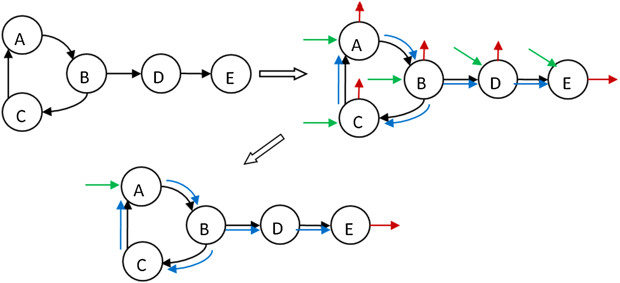
The construction procedure input. This figure demonstrates the translation of a “toy signaling network” to a list of reaction equations. Those equations will be used for model assembling according to the linear formulation.

FIG. 2.

Graphical representation of the inhibition parameter, αc. The inhibition parameter (αc) controls the inhibition “intensity” of the inhibitor (ν_c) on the “inhibited” reaction (ν_AB). determines the decline rate of flux as a function of the growth in flux. is affixed on a value between 1 (blue) and (red), and in the absence of prior biological information, the default inhibition intensity is fixed to (max suppression).

Second, the procedure applies an algorithm to detect and neutralize feedback loops that promote spurious stimulations (i.e., that allow stimulus in the absence of ligand). This algorithm requires prior definition of the network inputs set: stimulus initiators, or ligands.

Third, the next step is to generate a set of inward and outward flow reactions (i.e., exchange reactions) for some inner network species; these reactions are needed for preservation of the steady-state assumption. Therefore, we describe a novel optimization procedure for rigorous selection of proper exchange reactions.

Removing spurious stimulation loops

Positive and negative feedback loops are common and intrinsic features of signaling networks. Such loops, which have significant biological meaning, mostly occur in late stages of signaling cascades (i.e., after initial signal transduction). Their role can be positive (i.e., signal amplification) or negative (i.e., signal shutdown). These loops constitute a dynamic description of the signal cascade and therefore are able computationally to carry non-zero flux at steady state (Papin and Palsson, 2004a). Nevertheless, those feedback loops only have qualitative influence on signal transduction (i.e., they affect intensity but not presence of the signal), so their removal will not eliminate a model's ability to make certain types of predictions, namely qualitative ones. We distinguish between two types of cycles: “harmful” cycles, which may induce spurious signal activation without the presence of the proper stimulation (e.g., the ligand), and “harmless” loops, which have no disruptive effect on the model's predictions. Figure 3 illustrates examples for both harmful and harmless loops, based on interactions from Oda and Kitano (2006). Deceptive results caused by feedback loops is a common problem in signaling models that has mostly been treated through manual loop removal or correction (Li et al., 2009). We wish to eliminate only harmful loops via an automated procedure. Our strategy for doing so is to remove “non-essential” edges, that is, to refrain from removals that will fragment the connectivity between internal species and therefore cut off potential signaling pathways, but rather cut loops in the edges that will not create such disruptions on the network, and will rather specifically target the recycling species.

FIG. 3.

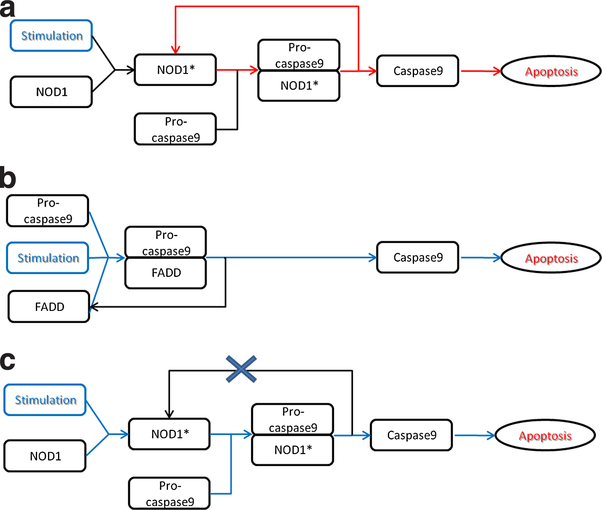
Examples of harmful and harmless feedback loops. This figure introduces two ways to activate apoptosis (Oda and Kitano, 2006). (a) Example of a harmful loop. In steady state, the internal non-zero flux (in red) is “activating” NOD1 without any stimulation, because the loop fully recovers the initial NOD1 species and therefore requires no net input of that biologically necessary substrate. (b) Harmless loop. The reaction between FADD and pro-caspase9 completely depends on the input stimulation (in blue). (c) Removal of the marked edge will guide apoptosis only upon an external stimulation.

Our loop removal procedure is based on a Depth-First Search (DFS) algorithm (Cormen, 2001), a classical method in which one of its applications is to identify cycles in a graph. The algorithm requires prior definition of the network's “stimulation” species set, which we define as inputs. Briefly, we perform a DFS from each stimulating species (Fig. 4a). In each step, products of the reaction are colored in gray (same as in the original DFS algorithm; Fig. 4b). Note that an edge to an already visited gray species indicates that this reaction closes a cycle (Fig. 4b). In practice, this “feedback” reaction neutralizes the necessity of a stimulus to initiate signal transduction in a steady-state. To eliminate this harmful cycle, the arc pointing to the gray species should be removed (Fig. 4c). Since each (hyper-) edge can have more than a single source or target, we avoid a second revisit of a reaction through another source by marking reactions as well upon visiting them (Fig. 4d).

FIG. 4.

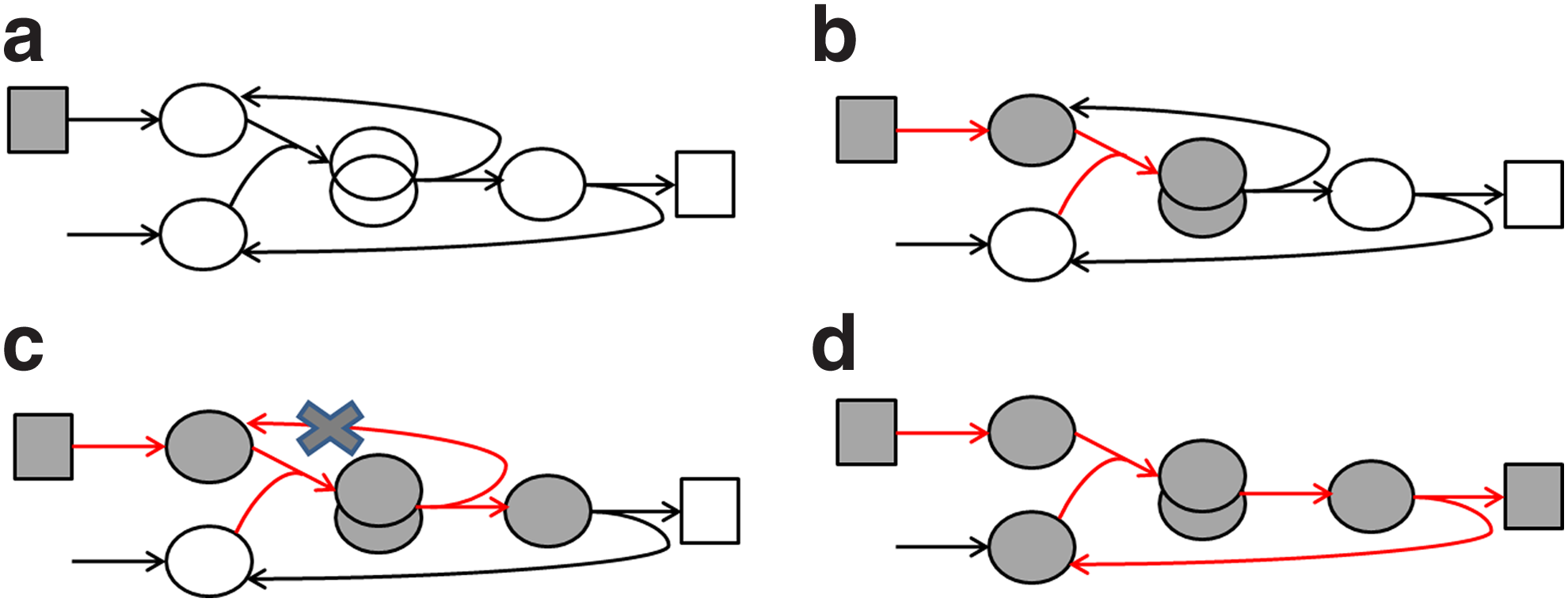
Illustration of the loop removal procedure. The algorithm starts from an input (a). In each subsequent step, newly discovered species are painted in gray (b), and examined reactions are marked (in red). (c) A reaction with an arc to a product which is already marked in gray is discovered. Therefore, the arc (and only it) will be removed. (d) The last step of the algorithm is illustrated.

Addition of proper exchange reactions

One of the requirements in CBM reconstruction is the addition of suitable “exchange reactions,” which are needed to maintain the steady-state and mass-balance constraints. In other words, those reactions allow substrate absorption into the system and by-product secretion (Duarte et al. 2004), enabling the flux flow through the network without the accumulation of metabolites.

Inputs of stimulus ligands are a subgroup of the model's exchange reactions set. They are unique among reactions in that they operate conditionally, depending on the presence of stimulus. To prevent confusion between input reactions of ligand to some input exchange reaction to inner species, we qualify input as refers only to input of stimulus or ligand.

To choose the exchange reactions in a rigorous way, we aim to find a set of inward and outward reactions that will allow all the internal reactions in the model to have non-zero fluxes through them, thereby ensuring that the model is consistent (Fig. 5). For this step, the inhibitions constraints are ignored, since they conflict with none-zero fluxes constraints for each internal reaction and therefore have no feasible solution. Formally, we define R_ex and R_in as the sets of all exchange and internal reactions, respectively. Then, we solve the following mixed-integer linear program to minimize the number of exchange reactions that are included in the final model (line 7). We emphasize that integer variables serve exclusively in the “model-building” stage and that simulations with the final model will be purely linear. \documentclass{aastex}\usepackage{amsbsy}\usepackage{amsfonts}\usepackage{amssymb}\usepackage{bm}\usepackage{mathrsfs}\usepackage{pifont}\usepackage{stmaryrd}\usepackage{textcomp}\usepackage{portland, xspace}\usepackage{amsmath, amsxtra}\pagestyle{empty}\DeclareMathSizes{10}{9}{7}{6}\begin{document} \begin{align*} & min \sum \nolimits_{i \in R_{ex}} w_i y_i \tag{7} \\ & s.t.\end{align*} \end{document} \documentclass{aastex}\usepackage{amsbsy}\usepackage{amsfonts}\usepackage{amssymb}\usepackage{bm}\usepackage{mathrsfs}\usepackage{pifont}\usepackage{stmaryrd}\usepackage{textcomp}\usepackage{portland, xspace}\usepackage{amsmath, amsxtra}\pagestyle{empty}\DeclareMathSizes{10}{9}{7}{6}\begin{document} \begin{align*} \quad\quad\quad& SV = 0 \tag{8} \\ & 0 \leq v_i \leq y_i v_{max} , \quad i \in R_{ex} \tag{9} \\ & y_i \in \{ 0 , 1 \} , \quad \quad \, i \in R_{ex} \tag{10} \\ & 1 \leq v_j \leq v_{max} , \qquad j \in R_{in} \tag{11} \end{align*} \end{document}

FIG. 5.

Choosing a minimal exchange reaction set. The figure illustrates the exchange reaction construction procedure. First, input and output reactions are added to each species. Second, the optimization procedure suggests some minimal selection for an exchange reaction set for a consistent model.

In this formulation, constraint (8) represents mass-balance. Constraints (9) and (10) define the integer variables for inclusion of each exchange reaction, and constraint (11) forces non-zero flux through internal reactions. The w_i weights allow prioritization of the reactions. In practice, we set each w_i to 1 (default value), but if we wish to minimize the selection of incoming exchange reaction to some species groups (for instance, phosphorylated or in complex proteins), we may impose a higher w_i to each ith species in those groups for choosing more biologically accurate solution.

Predicting system state

Since our formulation is based on purely linear constraints, it allows an unbiased sampling of feasible flux distributions given a particular set of inputs. Specifically, by sampling the space of feasible flux distributions and satisfying stoichiometric mass-balance (Price et al., 2004a) and model inhibition/activation constraints across N sampled solutions, we can compute the activation state of groups of species that we define as readouts or “experimentally observed” species under given stimulation.

We define a condition as a combination of model stimulations (i.e., the set of ligands for which input flux is allowed) with an additional possible combination of external perturbations of some inner network proteins (i.e., setting to zero the upper bounds of reactions that produce certain proteins).

Under each condition, we sampled the solution space N times, and isolated for each readout species the flux of their activation reaction (i.e., the reaction that produces the species' active formation). Then, a two-sample t-test was conducted in order to determine if the mean flux of each activation reaction is significantly different (with p-value ≤ 0.001) under the tested condition versus in the “lack of stimulus” condition. We found that to achieve meaningful statistics, N = 10³ is sufficient. For our analysis, we made use of COBRA Toolbox implementation for the randomized sampling procedure (Becker et al., 2007). In practice, calculating each separate condition requires several minutes of computing time, and serial testing of 31 different conditions takes a few hours (see Results). Due to the independence of the conditions, parallel computing can be employed and can reduce drastically the running time of the algorithm.

3. Results

Modeling EGFR signaling

We demonstrate our modeling framework on a large-scale map constructed by Oda et al. (2005) of the EGFR signaling pathway. EGFR is a central system regulating growth, survival, proliferation, and differentiations in mammalian cells (Samaga et al., 2009). The map contains 211 reactions and 322 species (including proteins, ions, simple molecules, oligomerrs, genes, and RNAs). Including all inhibition and activation constraints, the final CBM model contains 497 species and 694 reactions.

Comparison to Boolean approaches

In order to validate basic functionality of our method, we first compared the performance of our algorithm against that of a Boolean modeling approach (Hyduke and Palsson, 2010), which was recently applied to the EGFR system (Samaga et al., 2009), with respect to accuracy of predicting phenotypes of an in vivo phosphorylation dataset. The Boolean approach represents each node in the network using one of two possible states—active and inactive. The state of a node is derived from its “ancestors” in the network. While the Boolean formulation can effectively describe activation and inhibition rules, the linear model, as discussed above, is amenable to an assortment of tools that provide efficient and powerful model analysis options (Price et al., 2004a). We applied both methods to the original model of Oda et al. (2005), omitting additional species and reactions that were added in Samaga et al. (2009). We compare the two methods in their ability to predict the phenotypes of a phosphorylation data set, in which cells of the hepatocarcinoma cell line HepG2 were treated with a variety of drugs and growth factor alpha (TGFα) (Samaga et al., 2009), and the phoshorylation states of several proteins included in the EGFR network were measured. We use the normalized readout data supplied in Samaga et al. (2009), in which the activation states of 11 proteins are given binary values and assessed under 38 experimental conditions. Each condition represents a combination of stimulations (i.e., input ligands) and external perturbations of some inner network proteins. Our model is based purely on Oda et al. (2005), while the original Boolean model has integrated additional literature knowledge. As a result, we were able to test only 31 conditions and to monitor the activation states of only seven proteins.

On the tested conditions, we predicted the activation state of the seven readouts (see Methods). The Boolean model predicted correctly 68.7% of the states, while our approach achieved an accuracy rate of 75% (Fig. 6). The difference in performance is due to the difference between the model of Oda et al. (2005) that we used and that of Samaga et al. (2009), as described above. Nevertheless, focusing on prediction errors that are common to both models, it is possible to test the potential advantages of the linear formulation over the binary one, as its continuous representation may include useful information that is missing in the binary, discrete Boolean realization.

FIG. 6.

Performance evaluation. This table contains stimulations on HepG2 cells (Samaga et al., 2009). Each row represents a condition; for each of the readouts, there are two columns, representing the predictions of the CBM and Boolean models. Dark green, predicted correctly inactive; light green, predicted correctly active; dark red, predicted incorrectly inactive; light red, predicted incorrectly active. Black indicates that, on the tested condition, the readout was externally inhibited; therefore, its measurement was not relevant.

For instance, under some conditions, the protein PI3K is inhibited (marked in red in Fig. 7). As shown in Figure 7, this inhibition affects the activation level of Mek1/2 (flux is greater than 500 when PI3K is not inhibited and less than 500 when the inhibition takes place). Thus, while PI3K is not necessary for the activation of Mek1/2, it clearly affects it. Another example is the protein Creb (Fig. 8). In comparison to stimulation with p38 or PI3k inhibition, the inhibitions have a minor effect on Creb activation. Yet, we can notice that PI3k has a more decided influence (367.72 under PI3k versus 375.65). Network examination confirmed that PI3k is indeed located higher upstream to Creb than P38: thus, its inhibition effects on more pathways, which lead eventually to Creb activation. Such insights can be easily gleaned only from a continuous framework such as CBM.

FIG. 7.

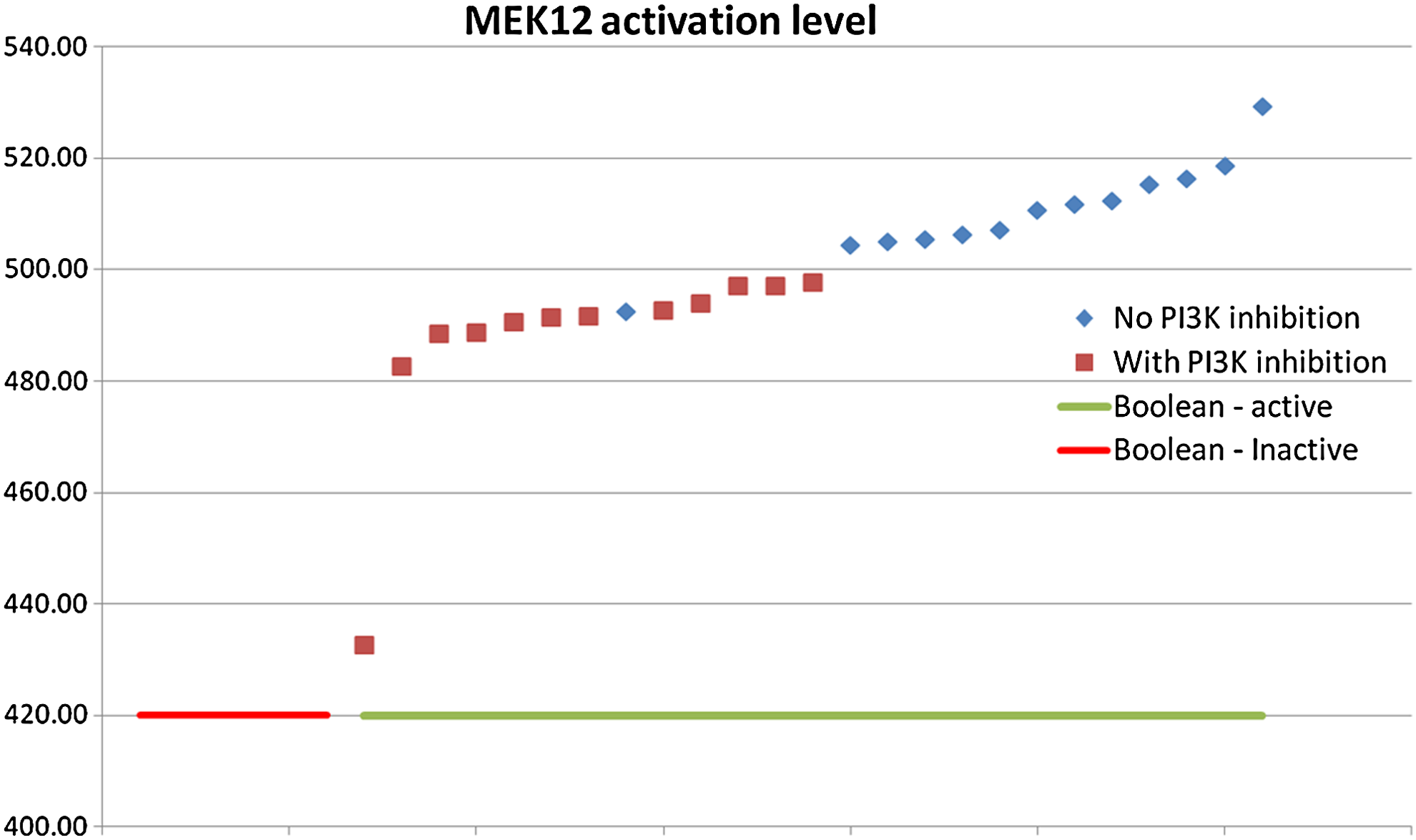
PI3K inhibition effect on MEK12. Each point indicates the activation level of MEK12 (i.e., the production rate of active MEK12) under a different condition. The red points indicate stimulus under PI3K inhibition. The points are sorted by the MEK12 activation flux level. The underlines indicate the Boolean predictions on each condition. While PI3K is not necessary for MEK12 activation (as seen from the Boolean results), it is clear that PI3K's inhibition negatively affects activation of MEK12. This conclusion cannot be deduced from the binary Boolean approach.

FIG. 8.

PI3K inhibition versus P38. In this figure, each data point indicates the activation level of Creb protein. The red point is a stimulation condition with PI3K inhibition, and the blue one is with P38 inhibition. The other conditions are marked with green. This comparison demonstrates that PI3K has more decisive effect on Creb activation level than P38.

4. Discussion

We devised a novel approach for modeling genome-scale signaling networks based on CBM (Dasika et al., 2006). The novelty of our formulation is the utilization of purely linear constraints, without relying on Integer programming in the modeling stage. The approach also supports graded constraints and variable strengths of activation and inhibition, which enables accurate capture of otherwise elusive phenotypes. Thus, our modeling approach allows the scale-up to large multi-variable networks. Our basic CBM formulation can be used to efficiently solve diversified optimization problems, relying on the existing tool-box for the analysis of genome-scale metabolism.

We introduce a comprehensive translation procedure to a signaling CBM, which can serve to reconstruct a working model for any given signaling system. The proposed procedure removes harmful feedback loops, which can generate spurious predictions, and rigorously chooses a minimal set of internal exchange reactions, which is needed to maintain the mass-balance CBM provision.

Having automatically constructed a linearized version of a given signaling network, we model the network effects of any given input condition by sampling the full spectrum of the resulting solution space derived from the given stimulation and/or perturbation. Even though our framework embodies strictly linear approximations in its run time, we show that it can be used to efficiently and accurately predict the in silico current state of the network species.

We demonstrate the reconstruction process by a translation of a detailed EGFR/ErbB map (Oda et al., 2005) to a CBM. We used a previous Boolean logic model and related phosphorylation data (Samaga et al., 2009) to validate the ability of our linear framework to model this system. Importantly, we show the power of uniform sampling of the solution space in providing informative predictions, emphasizing the utility of a linearized signaling CBM approach.

Our stimulation scheme, in combination with others' optimization machinery of CBM models, can be recruited to cope with a host of key questions, such as identifying system perturbations as potential drugs targets with minimal influence on other network species, marking new potential unknown interactions between system proteins in order to narrow experimental work, and suggesting new signaling pathways using gap-filling technologists.

Footnotes

Acknowledgments

We thank Tomer Benyamini, Keren Yitzchak, and Matthew Oberhardt for their support and for providing helpful feedback. This study was supported in part by a fellowship from the Edmond J. Safra Bioinformatics program at Tel-Aviv University. E.R. and R.S. were supported by a Bikura grant from the Israel Science Foundation.

Disclosure Statement

No competing financial interests exist.

References

Becker

S.A.

, Feist

A.M.

, Mo

M.L.

et al. 2007. Quantitative prediction of cellular metabolism with constraint-based models: the COBRA Toolbox. Nat. Protocols, 2:727–738.

Bornstein

B.J.

, Keating

S.M.

, Jouraku

et al. 2008. LibSBML: an API library for SBML. Bioinformatics, 24:880–881.

Cormen

T.H.

2001. Introduction to Algorithms. MIT Press: Cambridge, MA.

Dasika

M.S.

, Burgard

, Maranas

C.D.

2006. A computational framework for the topological analysis and targeted disruption of signal transduction networks. Biophys. J., 91:382–398.

Duarte

N.C.

, Herrgård

M.J.

, Palsson

2004. Reconstruction and validation of Saccharomyces cerevisiae iND750, a fully compartmentalized genome-scale metabolic model. Genome Res., 14:1298–1309.

Funahashi

, Morohashi

, Kitano

et al. 2003. CellDesigner: a process diagram editor for gene-regulatory and biochemical networks. BIOSILICO, 1:159–162.

Hyduke

D.R.

, Palsson

2010. Towards genome-scale signalling network reconstructions. Nat. Rev. Genet., 11:297–307.

Jerby

, Shlomi

, Ruppin

2010. Computational reconstruction of tissue-specific metabolic models: application to human liver metabolism. Mol. Syst. Biol., 6:401.

Kanehisa

, Goto

2000. KEGG: Kyoto Encyclopedia of Genes and Genomes. Nucleic Acids Res., 28:27–30.

10.

Karp

R.M.

American Mathematical Society, and Society for Industrial and Applied Mathematics. 1974. Complexity of Computation. American Mathematical Society: Providence, RI.

11.

, Thiele

, Jamshidi

et al. 2009. Identification of potential pathway mediation targets in Toll-like receptor signaling. PLoS Comput. Biol., 5:e1000292.

12.

Oda

, Kitano

2006. A comprehensive map of the toll-like receptor signaling network. Mol. Syst. Biol., 2:2006.0015.

13.

Oda

, Matsuoka

, Funahashi

et al. 2005. A comprehensive pathway map of epidermal growth factor receptor signaling. Mol. Syst. Biol., 1:2005.0010.

14.

Papin

J.A.

, Palsson

B.O.

2004a. The JAK-STAT signaling network in the human B-cell: an extreme signaling pathway analysis. Biophys. J., 87:37–46.

15.

Papin

J.A.

, Palsson

B.O.

2004b. Topological analysis of mass-balanced signaling networks: a framework to obtain network properties including crosstalk. J. Theor. Biol., 227:283–297.

16.

Price

N.D.

, Reed

J.L.

, Palsson

2004a. Genome-scale models of microbial cells: evaluating the consequences of constraints. Nat. Rev. Microbiol., 2:886–897.

17.

Price

N.D.

, Schellenberger

, Palsson

B.O.

2004b. Uniform sampling of steady-state flux spaces: means to design experiments and to interpret enzymopathies. Biophys. J., 87:2172–2186.

18.

Saez-Rodriguez

, Alexopoulos

L.G.

, Epperlein

et al. 2009. Discrete logic modelling as a means to link protein signalling networks with functional analysis of mammalian signal transduction. Mol. Syst. Biol., 5:331.

19.

Samaga

, Saez-Rodriguez

, Alexopoulos

L.G.

et al. 2009. The logic of EGFR/ErbB signaling: theoretical properties and analysis of high-throughput data. PLoS Comput. Biol., 5:e1000438.

20.

Steggles

L.J.

, Banks

, Shaw

et al. 2007. Qualitatively modelling and analysing genetic regulatory networks: a Petri net approach. Bioinformatics, 23:336–343.