The 5′-3′ Distance of RNA Secondary Structures

Abstract

Recently, Yoffe and colleagues observed that the average distances between 5′-3′ ends of RNA molecules are very small and largely independent of sequence length. This observation is based on numerical computations as well as theoretical arguments maximizing certain entropy functionals. In this article, we compute the exact distribution of 5′-3′ distances of RNA secondary structures for any finite n. Furthermore, we compute the limit distribution and show that for n = 30 the exact distribution and the limit distribution are very close. Our results show that the distances of random RNA secondary structures are distinctively lower than those of minimum free energy structures of random RNA sequences.

1. Introduction

The closeness of 5′ and 3′ ends of rna molecules has distinct biological significance, for instance, for the replication efficiency of single stranded RNA viruses or the efficient translation of messenger RNA molecules. It is speculated in Yoffe et al. (2011) that this effective circularization of large RNA molecules is rather a generic phenomenon of large RNA molecules and independent of sequence length. It is, to a large extent, attributed to the high number of paired bases.

In this article, we study the distribution of 5′-3′ distances in RNA secondary structures. We first compute the distribution of 5′-3′ distances of RNA secondary structures of length n by means of a bivariate generating function. The key idea is to view secondary structures as tableaux sequences and to relate the 5′-3′ distance to the nontrivial returns (Jin and Reidys, 2010b) of the corresponding path of shapes. Secondly, we derive the limit distribution of 5′-3′ distances. The idea is to compute the singular expansion of the above generating function via the subcritical paradigm (Flajolet and Sedgewick, 2009) and to employ a discrete limit theorem.

Our results prove that the 5′-3′ distances of random RNA structures are distinctively smaller than those of biological RNA molecules and minimum free energy (mfe) RNA structures. This comes as a surprise since the number of paired bases in random structures is 55.2% (Reidys, 2011) and therefore smaller than the 60% of mfe structures (Fontana et al., 1993).

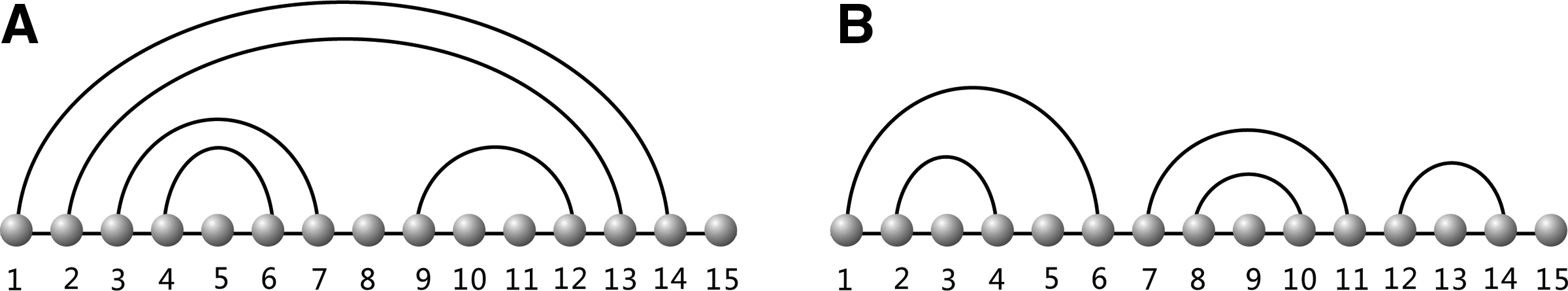
An RNA structure is the helical configuration of its primary sequence—i.e., the sequence of nucleotides A, G, U, and C, together with Watson-Crick (A-U, G-C) and (U-G) base pairs. The combinatorics of RNA secondary structures has been pioneered by Waterman and colleagues (Penner and Waterman, 1993; Waterman, 1978, 1979; Howell et al., 1980; Waterman and Schmitt, 1994). We interpret an RNA secondary structure as a diagram, i.e., labeled graphs over the vertex set \documentclass{aastex}\usepackage{amsbsy}\usepackage{amsfonts}\usepackage{amssymb}\usepackage{bm}\usepackage{mathrsfs}\usepackage{pifont}\usepackage{stmaryrd}\usepackage{textcomp}\usepackage{portland, xspace}\usepackage{amsmath, amsxtra}\pagestyle{empty}\DeclareMathSizes{10}{9}{7}{6}\begin{document}$$[ n ] = \{ 1 , \ldots , n \} $$\end{document} , represented by drawing its vertices \documentclass{aastex}\usepackage{amsbsy}\usepackage{amsfonts}\usepackage{amssymb}\usepackage{bm}\usepackage{mathrsfs}\usepackage{pifont}\usepackage{stmaryrd}\usepackage{textcomp}\usepackage{portland, xspace}\usepackage{amsmath, amsxtra}\pagestyle{empty}\DeclareMathSizes{10}{9}{7}{6}\begin{document}$$1 , \ldots , n$$\end{document} in a horizontal line and connecting them via the set of backbone-edges {(i, i + 1)′ ∣ 1 ≤ i ≤ n − 1}. Besides its backbone edges, a diagram exhibits arcs (i, j) that are drawn in the upper half-plane. Note that an arc of the form (i, i + 1) or 1-arc is distinguished from the backbone edge (i, i + 1)′. However, no confusion can arise since an RNA secondary structure is a diagram having no 1-arcs and only noncrossing arcs in the upper half-plane (Fig. 1).

FIG. 1.

RNA secondary structures as diagrams: the backbone of the RNA molecule is drawn as a horizontal line, and Watson-Crick base pairs are represented as arcs in the upper half-plane. An RNA secondary structure has no 1-arcs and only noncrossing arcs.

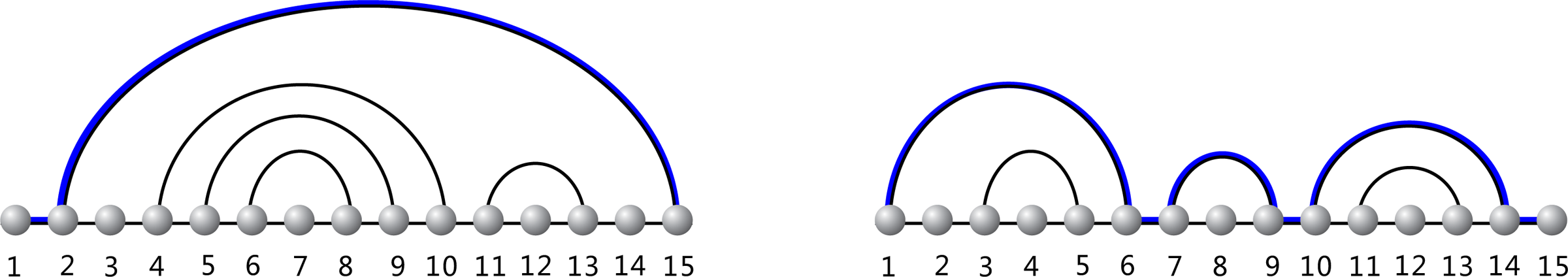
The 5′-3′ distance of an RNA secondary structure is the minimal length of a path of the diagram. Such a diagram-path is comprised of arcs and backbone-edges (Fig. 2).

FIG. 2.

The 5′-3′ distance of RNA secondary structures: distance contributing backbone-edges and arcs are drawn in blue. The structure on the lhs has 5′-3′ distance 2, and structure on the rhs has 5′-3′ distance 6.

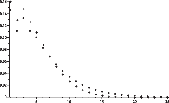
The article is organized as follows: In Section 2, we discuss some basic facts, in particular the structure-tableaux correspondence and how to express the 5′-3′ distance via such tableaux-sequences. In Section 3, we compute W(z, u), the bivariate generating function of RNA secondary structures of length n having distance d. Section 4 contains the computation of the singular expansion of W(z, u), and in Section 5 we combine our results and derive the limit distribution (Fig. 3). Finally, we discuss our results in Section 6.

FIG. 3.

The distribution of 5′-3′ distances of RNA secondary structures: We display the distribution of distances in RNA secondary structures of length 30 (+) derived via Theorem 1. We furthermore show the distribution of distances in the limit of long RNA secondary structures (•) obtained via Theorem 4.

2. Preliminaries

Let \documentclass{aastex}\usepackage{amsbsy}\usepackage{amsfonts}\usepackage{amssymb}\usepackage{bm}\usepackage{mathrsfs}\usepackage{pifont}\usepackage{stmaryrd}\usepackage{textcomp}\usepackage{portland, xspace}\usepackage{amsmath, amsxtra}\pagestyle{empty}\DeclareMathSizes{10}{9}{7}{6}\begin{document}$${ \cal S}_n$$\end{document} denote the set of RNA secondary structures of length n, σ_n. All results of this article easily generalize to the case of diagrams with noncrossing arcs that contain no arcs of length smaller than λ > 1 and to canonical secondary structures (Reidys, 2011), i.e., structures that contain no isolated arcs.

The distance of σ_n, d_n(σ_n), is the minimum length of a path consisting of σ-arcs and backbone-edges from vertex 1 (the 5′ end) to vertex n (the 3′-end). That is, we have the mapping \documentclass{aastex}\usepackage{amsbsy}\usepackage{amsfonts}\usepackage{amssymb}\usepackage{bm}\usepackage{mathrsfs}\usepackage{pifont}\usepackage{stmaryrd}\usepackage{textcomp}\usepackage{portland, xspace}\usepackage{amsmath, amsxtra}\pagestyle{empty}\DeclareMathSizes{10}{9}{7}{6}\begin{document}$$d_n : { \cal S}_n \longrightarrow {\mathbb N}$$\end{document} .

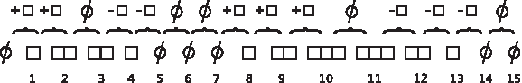
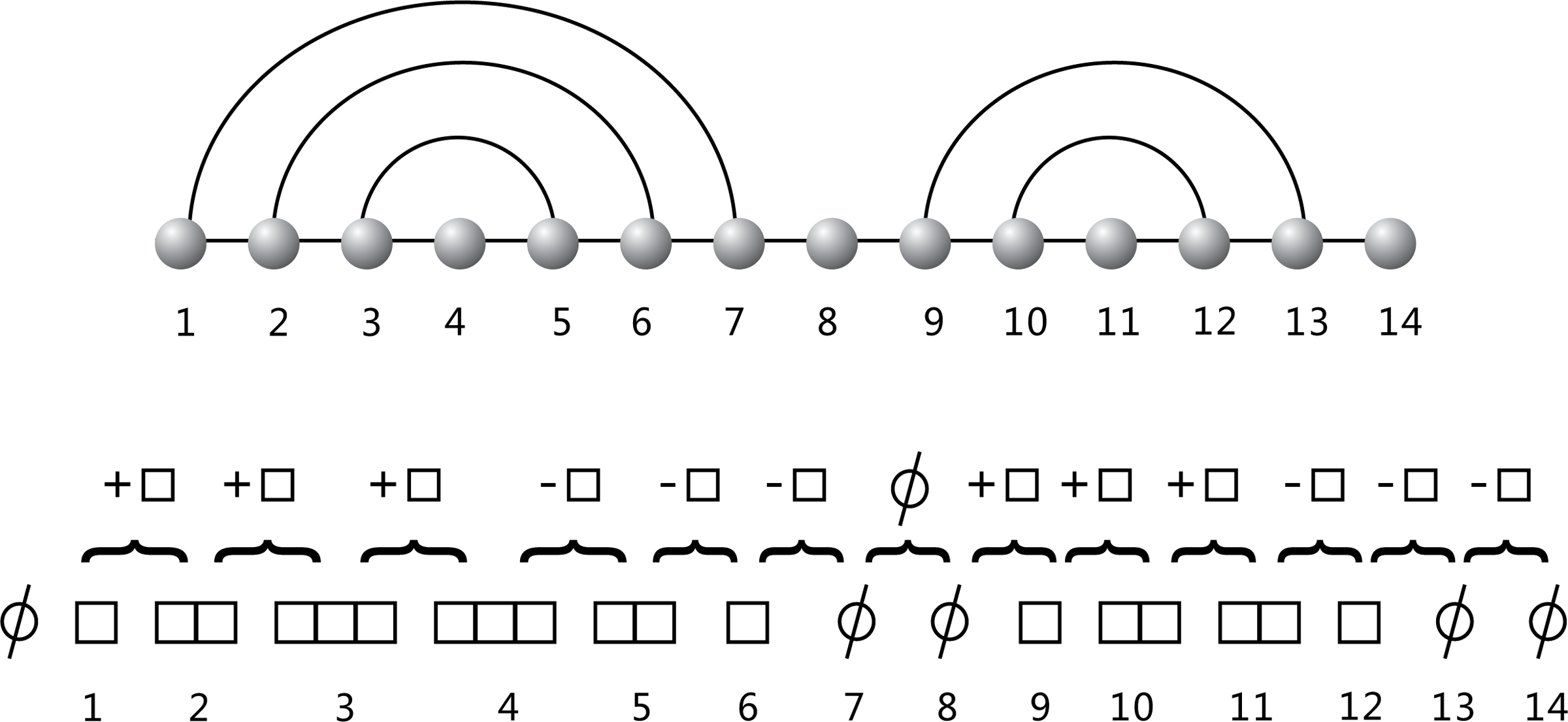
A sequence of shapes \documentclass{aastex}\usepackage{amsbsy}\usepackage{amsfonts}\usepackage{amssymb}\usepackage{bm}\usepackage{mathrsfs}\usepackage{pifont}\usepackage{stmaryrd}\usepackage{textcomp}\usepackage{portland, xspace}\usepackage{amsmath, amsxtra}\pagestyle{empty}\DeclareMathSizes{10}{9}{7}{6}\begin{document}$$( \lambda_0 , \lambda_1 , \ldots , \lambda_n )$$\end{document} is called a 1-tableaux of length n, T_n, if all shapes contain only one row of squares and (a) λ₀ = λ_n = Ø, (b) λ_i₊₁ is obtained from λ_i by adding a square (+□), removing a square (−□), or doing nothing (Ø) and (c) there exists no sequence of (+□, −□)-steps (Fig. 4). Let \documentclass{aastex}\usepackage{amsbsy}\usepackage{amsfonts}\usepackage{amssymb}\usepackage{bm}\usepackage{mathrsfs}\usepackage{pifont}\usepackage{stmaryrd}\usepackage{textcomp}\usepackage{portland, xspace}\usepackage{amsmath, amsxtra}\pagestyle{empty}\DeclareMathSizes{10}{9}{7}{6}\begin{document}$${ \cal T}_n$$\end{document} denote the set of all 1-tableaux of length n.

FIG. 4.

A 1-tableaux: at each step, either nothing happens or a single □ is added or removed.

We come next to the tableaux interpretation of secondary structures. The underlying correspondence is an immediate consequence of Chen et al. (2008, 2007) and Jin et al. (2008). We shall subsequently express the 5′-3′ distance via 1-tableaux.

Proposition 1

(Jin et al., 2008). There exists a bijection between RNA secondary structures and 1-tableaux: \documentclass{aastex}\usepackage{amsbsy}\usepackage{amsfonts}\usepackage{amssymb}\usepackage{bm}\usepackage{mathrsfs}\usepackage{pifont}\usepackage{stmaryrd}\usepackage{textcomp}\usepackage{portland, xspace}\usepackage{amsmath, amsxtra}\pagestyle{empty}\DeclareMathSizes{10}{9}{7}{6}\begin{document}\begin{align}\beta_n : { \cal S}_n \longrightarrow { \cal T}_n. \tag{2.1}\end{align}\end{document}

Proof

Given σ_n, we consider the sequence \documentclass{aastex}\usepackage{amsbsy}\usepackage{amsfonts}\usepackage{amssymb}\usepackage{bm}\usepackage{mathrsfs}\usepackage{pifont}\usepackage{stmaryrd}\usepackage{textcomp}\usepackage{portland, xspace}\usepackage{amsmath, amsxtra}\pagestyle{empty}\DeclareMathSizes{10}{9}{7}{6}\begin{document}$$( n , n - 1 , \ldots , 1 )$$\end{document} and, starting with Ø, do the following:
• if j is the endpoint of an arc (i, j), we add one square,

• if j is the start point of an arc (j, s), we remove one square,

• if j is an isolated point, we do nothing.

This constructs a 1-tableaux of length n and thus defines the map β_n (Fig. 5). Conversely, given a 1-tableau T_n, \documentclass{aastex}\usepackage{amsbsy}\usepackage{amsfonts}\usepackage{amssymb}\usepackage{bm}\usepackage{mathrsfs}\usepackage{pifont}\usepackage{stmaryrd}\usepackage{textcomp}\usepackage{portland, xspace}\usepackage{amsmath, amsxtra}\pagestyle{empty}\DeclareMathSizes{10}{9}{7}{6}\begin{document}$$(\O , {\lambda^1} , \ldots , \lambda^{n-1}, \O)$$\end{document} , reading λⁱ\λⁱ⁻¹ from left to right, at step i, we do the following:
• for a +□-step at i we insert i into the new square,

• for a Ø-step we do nothing,

• for a −□-step at i we extract the entry of the rightmost square j(i). The latter extractions generate the arc-set {(i, j(i)) ∣ i is a −□-step} that contains by definition of T_n no 1-arcs. Thus, this procedure generates a secondary structure of length n without 1-arc, which, by construction, is the inverse of β_n and the proposition follows. ■

FIG. 5.
Mapping RNA secondary structures into 1-tableaux.

A secondary structure σ_n is irreducible if β(σ_n) is a sequence of shapes \documentclass{aastex}\usepackage{amsbsy}\usepackage{amsfonts}\usepackage{amssymb}\usepackage{bm}\usepackage{mathrsfs}\usepackage{pifont}\usepackage{stmaryrd}\usepackage{textcomp}\usepackage{portland, xspace}\usepackage{amsmath, amsxtra}\pagestyle{empty}\DeclareMathSizes{10}{9}{7}{6}\begin{document}$$( \lambda_0 , \ldots , \lambda_{n} )$$\end{document} such that λ_j ≠ Ø for 1 ≤ j < n. An irreducible substructure of σ_n is a subsequence \documentclass{aastex}\usepackage{amsbsy}\usepackage{amsfonts}\usepackage{amssymb}\usepackage{bm}\usepackage{mathrsfs}\usepackage{pifont}\usepackage{stmaryrd}\usepackage{textcomp}\usepackage{portland, xspace}\usepackage{amsmath, amsxtra}\pagestyle{empty}\DeclareMathSizes{10}{9}{7}{6}\begin{document}$$( \lambda_i , \ldots , \lambda_{i + k} )$$\end{document} such that λ_i₋₁ = Ø and λ_i_+k = Ø and λ_j ≠ Ø for i ≤ j < i + k. In the following, we denote the terminal shapes (λ_i_+k) of non-rightmost irreducibles by Ø* and the terminal shape of the rightmost irreducible by Ø^#. Accordingly, we distinguish three types of shapes Ø, Ø* and Ø^#. We can now express the distance in terms of numbers of Ø* and Ø shapes as follows and see (Fig. 6) \documentclass{aastex}\usepackage{amsbsy}\usepackage{amsfonts}\usepackage{amssymb}\usepackage{bm}\usepackage{mathrsfs}\usepackage{pifont}\usepackage{stmaryrd}\usepackage{textcomp}\usepackage{portland, xspace}\usepackage{amsmath, amsxtra}\pagestyle{empty}\DeclareMathSizes{10}{9}{7}{6}\begin{document}\begin{align}d_n ( \sigma_n ) = 2 \mid \{\O^ \in \beta ( \sigma_n ) \} \mid + \mid \{ \O\in \beta ( \sigma_n ) \} \mid . \tag{2.2}\end{align}\end{document}

FIG. 6.
A secondary structure and its 1-tableaux: its 5′-3′ distance equals twice the number of Ø plus the number of Ø shapes, i.e., 2 × 2 + 4 = 8.

3. Combinatorial Analysis

Let w(n, d) denote the number of RNA secondary structures σ_n having distance d_n. In the following, we shall write d instead of d_n and consider \documentclass{aastex}\usepackage{amsbsy}\usepackage{amsfonts}\usepackage{amssymb}\usepackage{bm}\usepackage{mathrsfs}\usepackage{pifont}\usepackage{stmaryrd}\usepackage{textcomp}\usepackage{portland, xspace}\usepackage{amsmath, amsxtra}\pagestyle{empty}\DeclareMathSizes{10}{9}{7}{6}\begin{document}\begin{align}{ \bf W} ( z , u ) = \sum_{n \geq 0} \sum_{d \geq 0}{ \bf w} ( n , d ) z^n u^d , \tag{3.1}\end{align}\end{document}

the bivariate generating function of the number of RNA secondary structure of length n having distance d and set w(n) = ∑_d≥0w(n, d). Let S(z) denote the generating function of RNA secondary structures and Irr(z) denote the generating function of irreducible secondary structures (irreducibles). Furthermore, let \documentclass{aastex}\usepackage{amsbsy}\usepackage{amsfonts}\usepackage{amssymb}\usepackage{bm}\usepackage{mathrsfs}\usepackage{pifont}\usepackage{stmaryrd}\usepackage{textcomp}\usepackage{portland, xspace}\usepackage{amsmath, amsxtra}\pagestyle{empty}\DeclareMathSizes{10}{9}{7}{6}\begin{document}$${ \cal S}_n$$\end{document} denote the set of secondary structures of length n and \documentclass{aastex}\usepackage{amsbsy}\usepackage{amsfonts}\usepackage{amssymb}\usepackage{bm}\usepackage{mathrsfs}\usepackage{pifont}\usepackage{stmaryrd}\usepackage{textcomp}\usepackage{portland, xspace}\usepackage{amsmath, amsxtra}\pagestyle{empty}\DeclareMathSizes{10}{9}{7}{6}\begin{document}$${ \cal I}_n$$\end{document} denote the set of irreducible structures of length n.

Theorem 1

The bivariate generating function of the number of RNA secondary structures of length n with distance d, is given by \documentclass{aastex}\usepackage{amsbsy}\usepackage{amsfonts}\usepackage{amssymb}\usepackage{bm}\usepackage{mathrsfs}\usepackage{pifont}\usepackage{stmaryrd}\usepackage{textcomp}\usepackage{portland, xspace}\usepackage{amsmath, amsxtra}\pagestyle{empty}\DeclareMathSizes{10}{9}{7}{6}\begin{document}\begin{align} { \bf W } ( z , u ) = \frac { uz^2 ( { \bf S } ( z ) - 1 ) } { ( 1 - zu ) ^2 - ( 1 - zu ) ( zu ) ^2 ( { \bf S } ( z ) - 1 ) } + \frac { z } { 1 - zu } . \tag { 3.2 } \end{align}\end{document}

Proof

We set V(z, u) = z/(1 − zu) and U(z, u) = W(z, u) − V(z, u).

Claim 1

Irr(z) = z²(S(z) − 1).

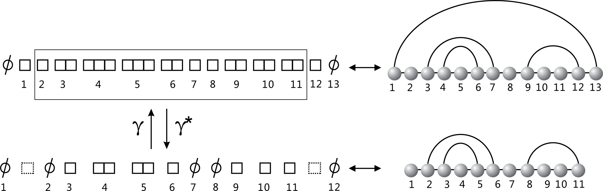
To prove Claim 1, we consider the mapping \documentclass{aastex}\usepackage{amsbsy}\usepackage{amsfonts}\usepackage{amssymb}\usepackage{bm}\usepackage{mathrsfs}\usepackage{pifont}\usepackage{stmaryrd}\usepackage{textcomp}\usepackage{portland, xspace}\usepackage{amsmath, amsxtra}\pagestyle{empty}\DeclareMathSizes{10}{9}{7}{6}\begin{document}$$\gamma: { \cal I}_n \longrightarrow { \cal S}_{n - 2}$$\end{document} , obtained by removing the shapes λ₁ and λ_n₋₁ from β(σ_n) and removing the rightmost box from all other shapes λ_j, 2 ≤ j ≤ n − 2. Note that for 1 =(n − 1) the tableaux β(σ_n) corresponds to a 1-arc which is impossible. Hence for an irreducible structure λ₁ = □ and λ_n₋₁ = □ are distinct shapes and the induced sequence of shapes \documentclass{aastex}\usepackage{amsbsy}\usepackage{amsfonts}\usepackage{amssymb}\usepackage{bm}\usepackage{mathrsfs}\usepackage{pifont}\usepackage{stmaryrd}\usepackage{textcomp}\usepackage{portland, xspace}\usepackage{amsmath, amsxtra}\pagestyle{empty}\DeclareMathSizes{10}{9}{7}{6}\begin{document}$$\mu = ( \lambda_0 , \lambda_2 \setminus \Box,\ldots , \lambda_{n - 2} \setminus\Box , \lambda_n )$$\end{document} is again a 1-tableaux, i.e., an element of \documentclass{aastex}\usepackage{amsbsy}\usepackage{amsfonts}\usepackage{amssymb}\usepackage{bm}\usepackage{mathrsfs}\usepackage{pifont}\usepackage{stmaryrd}\usepackage{textcomp}\usepackage{portland, xspace}\usepackage{amsmath, amsxtra}\pagestyle{empty}\DeclareMathSizes{10}{9}{7}{6}\begin{document}$${ \cal S}_{n - 2}$$\end{document} , where λ_j\□ denotes the shape λ_j with the rightmost □ deleted. Thus, γ is well defined. Given a 1-tableaux \documentclass{aastex}\usepackage{amsbsy}\usepackage{amsfonts}\usepackage{amssymb}\usepackage{bm}\usepackage{mathrsfs}\usepackage{pifont}\usepackage{stmaryrd}\usepackage{textcomp}\usepackage{portland, xspace}\usepackage{amsmath, amsxtra}\pagestyle{empty}\DeclareMathSizes{10}{9}{7}{6}\begin{document}$$\tau = ( \lambda_0 , \ldots , \lambda_{n - 2} )$$\end{document} we consider the map \documentclass{aastex}\usepackage{amsbsy}\usepackage{amsfonts}\usepackage{amssymb}\usepackage{bm}\usepackage{mathrsfs}\usepackage{pifont}\usepackage{stmaryrd}\usepackage{textcomp}\usepackage{portland, xspace}\usepackage{amsmath, amsxtra}\pagestyle{empty}\DeclareMathSizes{10}{9}{7}{6}\begin{document}\begin{align}\gamma^ ( \tau ) = ( \lambda_0 , \Box , \lambda_1 \sqcup \Box , \ldots , \lambda_{n - 3} \sqcup \Box , \Box , \lambda_{n - 2} ) \tag{3.3}\end{align}\end{document}

where λ_j* ⨆ □ denotes the shape λ_j with a □ added (Fig. 7).

FIG. 7.
The mappings γ and γ.

By construction, γ ∘ γ = id, whence Claim 1. Let us first compute the contribution of secondary structures containing at least one irreducible.

Claim 2

Suppose σ_n has distance d, then (i + 1) irreducibles can be arranged in exactly \documentclass{aastex}\usepackage{amsbsy}\usepackage{amsfonts}\usepackage{amssymb}\usepackage{bm}\usepackage{mathrsfs}\usepackage{pifont}\usepackage{stmaryrd}\usepackage{textcomp}\usepackage{portland, xspace}\usepackage{amsmath, amsxtra}\pagestyle{empty}\DeclareMathSizes{10}{9}{7}{6}\begin{document}$${d - i \choose i + 1}$$\end{document} ways.

Indeed, in view of \documentclass{aastex}\usepackage{amsbsy}\usepackage{amsfonts}\usepackage{amssymb}\usepackage{bm}\usepackage{mathrsfs}\usepackage{pifont}\usepackage{stmaryrd}\usepackage{textcomp}\usepackage{portland, xspace}\usepackage{amsmath, amsxtra}\pagestyle{empty}\DeclareMathSizes{10}{9}{7}{6}\begin{document}$$d = 2 \ , \mid \{\O^* \in \beta ( \sigma_n ) \} \mid + \mid \{\O\in \beta ( \sigma_n ) \} \mid$$\end{document} , the distance-contribution of the rightmost irreducible and each isolated point is one, while the contribution of all remaining i irreducibles equals two. No two such contributions overlap, whence replacing d by d − i we have ( \documentclass{aastex}\usepackage{amsbsy}\usepackage{amsfonts}\usepackage{amssymb}\usepackage{bm}\usepackage{mathrsfs}\usepackage{pifont}\usepackage{stmaryrd}\usepackage{textcomp}\usepackage{portland, xspace}\usepackage{amsmath, amsxtra}\pagestyle{empty}\DeclareMathSizes{10}{9}{7}{6}\begin{document}$${d - i \choose i + 1}$$\end{document} ) ways to place the (i + 1) irreducibles and Claim 2 follows. Accordingly, we obtain for fixed d \documentclass{aastex}\usepackage{amsbsy}\usepackage{amsfonts}\usepackage{amssymb}\usepackage{bm}\usepackage{mathrsfs}\usepackage{pifont}\usepackage{stmaryrd}\usepackage{textcomp}\usepackage{portland, xspace}\usepackage{amsmath, amsxtra}\pagestyle{empty}\DeclareMathSizes{10}{9}{7}{6}\begin{document}\begin{align}\sum_{n > d} { \bf u} ( n , d ) z^n = \sum_{i \geq 0}{d - i \choose i + 1} { \bf Irr} ( z ) ^{i + 1} z^{d - 2i - 1} , \tag{3.4}\end{align}\end{document}

where the indeterminant z corresponds to the isolated points and Irr(z) represents the irreducible structures labeled by the Ø* and Ø^#. Consequently, rearranging terms we derive \documentclass{aastex}\usepackage{amsbsy}\usepackage{amsfonts}\usepackage{amssymb}\usepackage{bm}\usepackage{mathrsfs}\usepackage{pifont}\usepackage{stmaryrd}\usepackage{textcomp}\usepackage{portland, xspace}\usepackage{amsmath, amsxtra}\pagestyle{empty}\DeclareMathSizes{10}{9}{7}{6}\begin{document}\begin{align}{ \bf U} ( z , u ) = \sum_{d \geq 1} \sum_{n > d} { \bf u} ( n , d ) z^n u^d = \sum_{i \geq 0} \sum_{d \geq 1} {d - i \choose i + 1} { \bf Irr} ( z ) ^{i + 1} z^{d - 2i - 1} u^d \tag{3.5}\end{align}\end{document}

and therefore \documentclass{aastex}\usepackage{amsbsy}\usepackage{amsfonts}\usepackage{amssymb}\usepackage{bm}\usepackage{mathrsfs}\usepackage{pifont}\usepackage{stmaryrd}\usepackage{textcomp}\usepackage{portland, xspace}\usepackage{amsmath, amsxtra}\pagestyle{empty}\DeclareMathSizes{10}{9}{7}{6}\begin{document}\begin{align} {\bf U} (z , u) & = \sum_ {i \geq 0} \sum_ {d \geq 1} {d - i \choose i + 1} (zu) ^ {d - i} (z) ^ {- i - 1} u^i \ {\bf Irr} (z) ^ {i + 1} \\ & = \sum_ {i \geq 0} \sum_ {d \geq 1} {d - i \choose i + 1} (zu) ^ {d - i} \left(\frac {u {\bf Irr} (z)} {z} \right) ^i \ \frac {{\bf Irr} (z)} {z} . \tag {3.6} \end{align}\end{document}

Using \documentclass{aastex}\usepackage{amsbsy}\usepackage{amsfonts}\usepackage{amssymb}\usepackage{bm}\usepackage{mathrsfs}\usepackage{pifont}\usepackage{stmaryrd}\usepackage{textcomp}\usepackage{portland, xspace}\usepackage{amsmath, amsxtra}\pagestyle{empty}\DeclareMathSizes{10}{9}{7}{6}\begin{document}$$ \sum\nolimits_ {r \geq 0} {r \choose k} x^r = \frac {x^k} {(1 - x) ^ {k + 1}} , k \geq 0$$\end{document} , we compute \documentclass{aastex}\usepackage{amsbsy}\usepackage{amsfonts}\usepackage{amssymb}\usepackage{bm}\usepackage{mathrsfs}\usepackage{pifont}\usepackage{stmaryrd}\usepackage{textcomp}\usepackage{portland, xspace}\usepackage{amsmath, amsxtra}\pagestyle{empty}\DeclareMathSizes{10}{9}{7}{6}\begin{document}\begin{align} {\bf U} (z , u) & = \sum_ {i \geq 0} \frac {(zu) ^ {i + 1}} {(1 - zu) ^ {i + 2}} \left(\frac {u {\bf Irr} (z)} {z} \right) ^i \ \frac {{\bf Irr} (z)} {z} \\ & = \frac {1} {1 - \frac {zu} {1 - zu} \frac {u {\bf Irr} (z)} {z}} \frac {zu {\bf Irr} (z)} {z (1 - zu) ^2} \\ & = \frac {uz^2 ({\bf S} (z) - 1)} {(1 - zu) ^2 - (1 - zu) z^2u^2 ({\bf S} (z) - 1)} . \tag { 3.7 } \end{align}\end{document}

It remains to consider RNA secondary structures that contain no irreducibles, i.e., RNA secondary structures consisting exclusively of isolated vertices. Clearly, \documentclass{aastex}\usepackage{amsbsy}\usepackage{amsfonts}\usepackage{amssymb}\usepackage{bm}\usepackage{mathrsfs}\usepackage{pifont}\usepackage{stmaryrd}\usepackage{textcomp}\usepackage{portland, xspace}\usepackage{amsmath, amsxtra}\pagestyle{empty}\DeclareMathSizes{10}{9}{7}{6}\begin{document}\begin{align} { \bf V } ( z , u ) = \sum_ { n \geq 1 } z^n u^ { n - 1 } = \frac { z } { 1 - zu } \end{align}\end{document}

and the proof of the theorem is complete. ■

Setting p(n, d) = w(n, d)/w(n), Theorem 1 provides the distribution of distances for RNA secondary structures of any fixed length, n (Table 1).

Table 1.
Distribution of Distances of RNA Secondary Structures of Length 30

d 1 2 3 4 5 6

p(n, d) 0.161 0.129 0.148 0.126 0.109 0.088

d 7 8 9 10 11 12

p(n, d) 0.069 5.18 × 10⁻² 3.8 × 10⁻² 2.71 × 10⁻² 1.87 × 10⁻² 1.26 × 10⁻²

d 13 14 15 16 17 18

p(n, d) 8.22 × 10⁻³ 5.19 × 10⁻³ 3.17 × 10⁻³ 1.86 × 10⁻³ 1.05 × 10⁻³ 5.62 × 10⁻⁴

d 19 20 21 22 23 24

p(n, d) 2.85 × 10⁻⁴ 1.36 × 10⁻⁴ 5.99 × 10⁻⁵ 2.41 × 10⁻⁵ 8.58 × 10⁻⁶ 2.63 × 10⁻⁶

d 25 26 27 28 29

p(n, d) 6.56 × 10⁻⁷ 1.24 × 10⁻⁷ 1.64 × 10⁻⁸ 1.30 × 10⁻⁹ 4.65 × 10⁻¹¹

The data of this table are represented in Fig. 3 as “+.”

4. The Singular Expansion

In this section, we analyze the asymptotics of the nth coefficient, [zⁿ]W(z, u). This will play a crucial role for the computation of the limit distribution of distances in Section 5.

Let us first establish some facts needed for deriving the singular expansion:

Lemma 1

W(z, u) is algebraic over the rational function field \documentclass{aastex}\usepackage{amsbsy}\usepackage{amsfonts}\usepackage{amssymb}\usepackage{bm}\usepackage{mathrsfs}\usepackage{pifont}\usepackage{stmaryrd}\usepackage{textcomp}\usepackage{portland, xspace}\usepackage{amsmath, amsxtra}\pagestyle{empty}\DeclareMathSizes{10}{9}{7}{6}\begin{document}$${\mathbb C} ( z , u )$$\end{document} and has the unique dominant singularity, \documentclass{aastex}\usepackage{amsbsy}\usepackage{amsfonts}\usepackage{amssymb}\usepackage{bm}\usepackage{mathrsfs}\usepackage{pifont}\usepackage{stmaryrd}\usepackage{textcomp}\usepackage{portland, xspace}\usepackage{amsmath, amsxtra}\pagestyle{empty}\DeclareMathSizes{10}{9}{7}{6}\begin{document}$$\rho = ( 3 - \sqrt{5} ) / 2$$\end{document} , which coincides with the unique dominant singularity of S(z).

Proof

The fact that W(z, u) is algebraic over the rational function \documentclass{aastex}\usepackage{amsbsy}\usepackage{amsfonts}\usepackage{amssymb}\usepackage{bm}\usepackage{mathrsfs}\usepackage{pifont}\usepackage{stmaryrd}\usepackage{textcomp}\usepackage{portland, xspace}\usepackage{amsmath, amsxtra}\pagestyle{empty}\DeclareMathSizes{10}{9}{7}{6}\begin{document}$${\mathbb C} ( z , u )$$\end{document} follows immediately from Theorem 1, where we proved \documentclass{aastex}\usepackage{amsbsy}\usepackage{amsfonts}\usepackage{amssymb}\usepackage{bm}\usepackage{mathrsfs}\usepackage{pifont}\usepackage{stmaryrd}\usepackage{textcomp}\usepackage{portland, xspace}\usepackage{amsmath, amsxtra}\pagestyle{empty}\DeclareMathSizes{10}{9}{7}{6}\begin{document}\begin{align} { \bf W } ( z , u ) = \frac { uz^2 ( { \bf S } ( z ) - 1 ) } { ( 1 - zu ) ^2 - ( 1 - zu ) ( zu ) ^2 ( { \bf S } ( z ) - 1 ) } + \frac { z } { 1 - zu } ,\end{align}\end{document}

since evidently all nominators and denominators are polynomial expressions in u and z and \documentclass{aastex}\usepackage{amsbsy}\usepackage{amsfonts}\usepackage{amssymb}\usepackage{bm}\usepackage{mathrsfs}\usepackage{pifont}\usepackage{stmaryrd}\usepackage{textcomp}\usepackage{portland, xspace}\usepackage{amsmath, amsxtra}\pagestyle{empty}\DeclareMathSizes{10}{9}{7}{6}\begin{document}\begin{align} { \bf S } ( z ) = \frac { 1 - z + z^2 - \sqrt { ( z^2 + z + 1 ) ( z^2 - 3 z + 1 ) } } { 2z^2 } . \tag { 4.1 } \end{align}\end{document}

Thus, the field \documentclass{aastex}\usepackage{amsbsy}\usepackage{amsfonts}\usepackage{amssymb}\usepackage{bm}\usepackage{mathrsfs}\usepackage{pifont}\usepackage{stmaryrd}\usepackage{textcomp}\usepackage{portland, xspace}\usepackage{amsmath, amsxtra}\pagestyle{empty}\DeclareMathSizes{10}{9}{7}{6}\begin{document}$${\mathbb C} ( z , u ) [ { \bf S} ( z ) ]$$\end{document} is algebraic of degree two over \documentclass{aastex}\usepackage{amsbsy}\usepackage{amsfonts}\usepackage{amssymb}\usepackage{bm}\usepackage{mathrsfs}\usepackage{pifont}\usepackage{stmaryrd}\usepackage{textcomp}\usepackage{portland, xspace}\usepackage{amsmath, amsxtra}\pagestyle{empty}\DeclareMathSizes{10}{9}{7}{6}\begin{document}$${\mathbb C} ( z , u )$$\end{document} . The second assertion follows from \documentclass{aastex}\usepackage{amsbsy}\usepackage{amsfonts}\usepackage{amssymb}\usepackage{bm}\usepackage{mathrsfs}\usepackage{pifont}\usepackage{stmaryrd}\usepackage{textcomp}\usepackage{portland, xspace}\usepackage{amsmath, amsxtra}\pagestyle{empty}\DeclareMathSizes{10}{9}{7}{6}\begin{document}$$u \in ( 0 , 1 )$$\end{document} and a straightforward analysis of the singularities of the two denominators (1 − zu)² − (1 −zu)(zu)²(S(z) − 1) and (1 − zu). ■

Given two numbers φ, r, where r > |κ| and \documentclass{aastex}\usepackage{amsbsy}\usepackage{amsfonts}\usepackage{amssymb}\usepackage{bm}\usepackage{mathrsfs}\usepackage{pifont}\usepackage{stmaryrd}\usepackage{textcomp}\usepackage{portland, xspace}\usepackage{amsmath, amsxtra}\pagestyle{empty}\DeclareMathSizes{10}{9}{7}{6}\begin{document}$$0 < \phi < \frac { \pi } { 2 } $$\end{document} , the open domain Δ_κ(φ, r) is defined as \documentclass{aastex}\usepackage{amsbsy}\usepackage{amsfonts}\usepackage{amssymb}\usepackage{bm}\usepackage{mathrsfs}\usepackage{pifont}\usepackage{stmaryrd}\usepackage{textcomp}\usepackage{portland, xspace}\usepackage{amsmath, amsxtra}\pagestyle{empty}\DeclareMathSizes{10}{9}{7}{6}\begin{document}\begin{align}\Delta_ \kappa ( \phi , r ) = \{ z \mid \ \mid z \mid < r , z \neq \kappa , \mid { \rm Arg} ( z - \kappa ) \mid > \phi \} .\end{align}\end{document}

A domain is a Δ_κ-domain at κ if it is of the form Δ_κ(φ, r) for some r and φ. A function is Δ_κ-analytic if it is analytic in some Δ_κ-domain.

Suppose an algebraic function has a unique singularity κ. According to Flajolet and Sedgewick (2009) and Stanley (1980), such a function is Δ_κ(φ, r)-analytic. In particular, W(z, u) is Δ_ρ(φ, r)-analytic. We introduce the notation \documentclass{aastex}\usepackage{amsbsy}\usepackage{amsfonts}\usepackage{amssymb}\usepackage{bm}\usepackage{mathrsfs}\usepackage{pifont}\usepackage{stmaryrd}\usepackage{textcomp}\usepackage{portland, xspace}\usepackage{amsmath, amsxtra}\pagestyle{empty}\DeclareMathSizes{10}{9}{7}{6}\begin{document}\begin{align}\left( f ( z ) = o \left( g ( z ) \right) \ \hbox{as} \ z \rightarrow \kappa \right) \leftrightarrow \left( f ( z ) / g ( z ) \rightarrow 0 \ \hbox{as} \ z \rightarrow \kappa \right) ,\end{align}\end{document}

and if we write f (z) = o(g(z)), it is implicitly assumed that z tends to the (unique) singularity. The following transfer theorem allows us to obtain the asymptotics of the coefficients from the generating functions.

Theorem 2

(Flajolet and Sedgewick, 2009). Let f (z) be a Δ_κ-analytic function at its unique singularity z = κ. Let \documentclass{aastex}\usepackage{amsbsy}\usepackage{amsfonts}\usepackage{amssymb}\usepackage{bm}\usepackage{mathrsfs}\usepackage{pifont}\usepackage{stmaryrd}\usepackage{textcomp}\usepackage{portland, xspace}\usepackage{amsmath, amsxtra}\pagestyle{empty}\DeclareMathSizes{10}{9}{7}{6}\begin{document}$$g ( z ) \in \{ ( \kappa - z ) ^{ \alpha} \mid \alpha \in {\mathbb R} \} $$\end{document} . Suppose we have in the intersection of a neighborhood of κ with the Δ_κ-domain \documentclass{aastex}\usepackage{amsbsy}\usepackage{amsfonts}\usepackage{amssymb}\usepackage{bm}\usepackage{mathrsfs}\usepackage{pifont}\usepackage{stmaryrd}\usepackage{textcomp}\usepackage{portland, xspace}\usepackage{amsmath, amsxtra}\pagestyle{empty}\DeclareMathSizes{10}{9}{7}{6}\begin{document}\begin{align}f ( z ) = o ( g ( z ) ) \quad {for }\ z \rightarrow \kappa.\end{align}\end{document}

Then we have \documentclass{aastex}\usepackage{amsbsy}\usepackage{amsfonts}\usepackage{amssymb}\usepackage{bm}\usepackage{mathrsfs}\usepackage{pifont}\usepackage{stmaryrd}\usepackage{textcomp}\usepackage{portland, xspace}\usepackage{amsmath, amsxtra}\pagestyle{empty}\DeclareMathSizes{10}{9}{7}{6}\begin{document}\begin{align}[ z^n ] f ( z ) = o \left( [ z^n ] g ( z ) \right) .\end{align}\end{document}

In addition, according to Flajolet et al. (2005), we have for \documentclass{aastex}\usepackage{amsbsy}\usepackage{amsfonts}\usepackage{amssymb}\usepackage{bm}\usepackage{mathrsfs}\usepackage{pifont}\usepackage{stmaryrd}\usepackage{textcomp}\usepackage{portland, xspace}\usepackage{amsmath, amsxtra}\pagestyle{empty}\DeclareMathSizes{10}{9}{7}{6}\begin{document}$$\alpha \in{\mathbb C} \setminus {\mathbb Z}_{ \le 0} :$$\end{document} \documentclass{aastex}\usepackage{amsbsy}\usepackage{amsfonts}\usepackage{amssymb}\usepackage{bm}\usepackage{mathrsfs}\usepackage{pifont}\usepackage{stmaryrd}\usepackage{textcomp}\usepackage{portland, xspace}\usepackage{amsmath, amsxtra}\pagestyle{empty}\DeclareMathSizes{10}{9}{7}{6}\begin{document}\begin{align}[ z^n ] , ( 1 - z ) ^ { - \alpha } \ \sim \frac { n^ { \alpha - 1 } } { \Gamma ( \alpha ) } \left[ 1 + \frac { \alpha ( \alpha - 1 ) } { 2n } + O \left( \frac { 1 } { n^2 } \right) \right] . \tag { 4.2 } \end{align}\end{document}

We next observe W(z, u) = h(z, u) f (g(z, u)), where g(z, u) = (uz²(S(z) − 1))/(1 − uz), f (z) = z/(1 − uz), h(z, u) = 1/(1 − zu) and t(z, u) = uz²/(1 − uz). In preparation for the proof of Lemma 2, we set \documentclass{aastex}\usepackage{amsbsy}\usepackage{amsfonts}\usepackage{amssymb}\usepackage{bm}\usepackage{mathrsfs}\usepackage{pifont}\usepackage{stmaryrd}\usepackage{textcomp}\usepackage{portland, xspace}\usepackage{amsmath, amsxtra}\pagestyle{empty}\DeclareMathSizes{10}{9}{7}{6}\begin{document}\begin{align} & \alpha = g (\rho , u) = \frac {2 (- 2 + \sqrt {5})u} {2 + (- 3 + \sqrt {5}) u} \\ & C_0 = \frac {2} {2 - (3 - \sqrt {5}) u} \\& \quad \left(f (\alpha) + \frac {d f (w)} {d w} \left | _ {w = \alpha} t (\rho , u) \frac {\sqrt {5} - 1} {3 - \sqrt {5}} - \alpha \frac {d f (w)} {d w} \right | _ {w = \alpha} + \rho \right) \\& r (\rho , u) = - \frac {2} {2 - (3 - \sqrt {5}) u} \frac {d f (w)} {d w} \left | _ {w = \alpha} t (\rho , u) \frac {\sqrt {8 (3 \sqrt {5} - 5)}} {(- 3 + \sqrt {5}) ^2} \right . . \end{align}\end{document}

Furthermore, let v(z) and w(z) be D-finite power series such that w(0) = 0 and let ρ_v, ρ_w denote their respective radius of convergence. We set \documentclass{aastex}\usepackage{amsbsy}\usepackage{amsfonts}\usepackage{amssymb}\usepackage{bm}\usepackage{mathrsfs}\usepackage{pifont}\usepackage{stmaryrd}\usepackage{textcomp}\usepackage{portland, xspace}\usepackage{amsmath, amsxtra}\pagestyle{empty}\DeclareMathSizes{10}{9}{7}{6}\begin{document}$$\tau_w = \lim \nolimits _{z \rightarrow \rho_w^{ - }} w ( z )$$\end{document} and call the D-finite power series F(z) = v(w(z)) subcritical if and only if τ_w < ρ_v.

Lemma 2

The singular expansion of W(z, u) at its unique, dominant singularity ρ is given by \documentclass{aastex}\usepackage{amsbsy}\usepackage{amsfonts}\usepackage{amssymb}\usepackage{bm}\usepackage{mathrsfs}\usepackage{pifont}\usepackage{stmaryrd}\usepackage{textcomp}\usepackage{portland, xspace}\usepackage{amsmath, amsxtra}\pagestyle{empty}\DeclareMathSizes{10}{9}{7}{6}\begin{document}\begin{align}{ \bf W} ( z , u ) = C_0 + { \bf V} ( \rho , u ) + r ( \rho , u ) ( \rho - z ) ^{1 / 2} + O ( \rho - z ) . \tag{4.3}\end{align}\end{document}

Proof

Since g(0, u) = 0, the composition f (g(z, u)) is well defined as a formal power series and \documentclass{aastex}\usepackage{amsbsy}\usepackage{amsfonts}\usepackage{amssymb}\usepackage{bm}\usepackage{mathrsfs}\usepackage{pifont}\usepackage{stmaryrd}\usepackage{textcomp}\usepackage{portland, xspace}\usepackage{amsmath, amsxtra}\pagestyle{empty}\DeclareMathSizes{10}{9}{7}{6}\begin{document}$$ { \bf V } ( z , u ) = \frac { z } { 1 - zu } $$\end{document} as well as h(z, u) are regular at ρ. Since \documentclass{aastex}\usepackage{amsbsy}\usepackage{amsfonts}\usepackage{amssymb}\usepackage{bm}\usepackage{mathrsfs}\usepackage{pifont}\usepackage{stmaryrd}\usepackage{textcomp}\usepackage{portland, xspace}\usepackage{amsmath, amsxtra}\pagestyle{empty}\DeclareMathSizes{10}{9}{7}{6}\begin{document}$$u \in ( 0 , 1 )$$\end{document} we have 1/u > 1 > ρ, whence the dominant singularity of g(z, u) equals ρ. Next we observe \documentclass{aastex}\usepackage{amsbsy}\usepackage{amsfonts}\usepackage{amssymb}\usepackage{bm}\usepackage{mathrsfs}\usepackage{pifont}\usepackage{stmaryrd}\usepackage{textcomp}\usepackage{portland, xspace}\usepackage{amsmath, amsxtra}\pagestyle{empty}\DeclareMathSizes{10}{9}{7}{6}\begin{document}\begin{align}g ( \rho , u ) = \frac { u ( 1 - \rho - \rho^2 ) } { 2 ( 1 - u \rho ) } < \frac { 0.7 u } { 2 ( 1 - 0.4u ) } = \frac { 0.35u } { 1 - 0.4u } < 1 ,\end{align}\end{document}

whence f (g(z, u)) is governed by the subcritical paradigm.

Claim 1. \documentclass{aastex}\usepackage{amsbsy}\usepackage{amsfonts}\usepackage{amssymb}\usepackage{bm}\usepackage{mathrsfs}\usepackage{pifont}\usepackage{stmaryrd}\usepackage{textcomp}\usepackage{portland, xspace}\usepackage{amsmath, amsxtra}\pagestyle{empty}\DeclareMathSizes{10}{9}{7}{6}\begin{document}\begin{align}g ( z , u ) = t ( \rho , u ) \frac { 2 } { 3 - \sqrt { 5 } } - t ( \rho , u ) \frac { \sqrt { 8 ( 3 \sqrt { 5 } - 5 ) ( \rho - z ) } } { ( - 3 + \sqrt { 5 } ) ^2 } + O ( \rho - z ) . \tag { 4.4 } \end{align}\end{document}

To prove the claim, we consider the singular expansion of S(z) at ρ \documentclass{aastex}\usepackage{amsbsy}\usepackage{amsfonts}\usepackage{amssymb}\usepackage{bm}\usepackage{mathrsfs}\usepackage{pifont}\usepackage{stmaryrd}\usepackage{textcomp}\usepackage{portland, xspace}\usepackage{amsmath, amsxtra}\pagestyle{empty}\DeclareMathSizes{10}{9}{7}{6}\begin{document}\begin{align} { \bf S } ( z ) = \frac { 2 } { 3 - \sqrt { 5 } } - \frac { \sqrt { 8 ( 3 \sqrt { 5 } - 5 ) ( \rho - z ) } } { ( - 3 + \sqrt { 5 } ) ^2 } + O ( \rho - z ) . \tag { 4.5 } \end{align}\end{document}

The singular expansion of g(z, u) at ρ is obtained by multiplying the regular expansion of t(z, u) and singular expansion of S(z) − 1. Clearly, \documentclass{aastex}\usepackage{amsbsy}\usepackage{amsfonts}\usepackage{amssymb}\usepackage{bm}\usepackage{mathrsfs}\usepackage{pifont}\usepackage{stmaryrd}\usepackage{textcomp}\usepackage{portland, xspace}\usepackage{amsmath, amsxtra}\pagestyle{empty}\DeclareMathSizes{10}{9}{7}{6}\begin{document}\begin{align}t ( z , u ) = t ( \rho , u ) - \frac { d t ( z , u ) } { dz } \Bigg | _ { z = \rho } ( \rho - z ) + O ( ( \rho - z ) ^2 ) , \tag { 4.6 } \end{align}\end{document}

where \documentclass{aastex}\usepackage{amsbsy}\usepackage{amsfonts}\usepackage{amssymb}\usepackage{bm}\usepackage{mathrsfs}\usepackage{pifont}\usepackage{stmaryrd}\usepackage{textcomp}\usepackage{portland, xspace}\usepackage{amsmath, amsxtra}\pagestyle{empty}\DeclareMathSizes{10}{9}{7}{6}\begin{document}$${\rm t}( \rho , u ) = ( 7 - 3 \sqrt{5} ) u / ( 2 - ( 3 - \sqrt{5} ) u )$$\end{document} . Thus \documentclass{aastex}\usepackage{amsbsy}\usepackage{amsfonts}\usepackage{amssymb}\usepackage{bm}\usepackage{mathrsfs}\usepackage{pifont}\usepackage{stmaryrd}\usepackage{textcomp}\usepackage{portland, xspace}\usepackage{amsmath, amsxtra}\pagestyle{empty}\DeclareMathSizes{10}{9}{7}{6}\begin{document}\begin{align}g ( z , u ) = t ( \rho , u ) \frac { \sqrt { 5 } - 1 } { 3 - \sqrt { 5 } } - t ( \rho , u ) \frac { \sqrt { 8 ( 3 \sqrt { 5 } - 5 ) ( \rho - z ) } } { ( - 3 + \sqrt { 5 } ) ^2 } + O ( \rho - z ) . \tag { 4.7 } \end{align}\end{document}

Setting \documentclass{aastex}\usepackage{amsbsy}\usepackage{amsfonts}\usepackage{amssymb}\usepackage{bm}\usepackage{mathrsfs}\usepackage{pifont}\usepackage{stmaryrd}\usepackage{textcomp}\usepackage{portland, xspace}\usepackage{amsmath, amsxtra}\pagestyle{empty}\DeclareMathSizes{10}{9}{7}{6}\begin{document}$$\alpha = g ( \rho , u ) = 2 ( - 2 + \sqrt{5} ) u / ( 2 + ( - 3 + \sqrt{5} ) u )$$\end{document} , the regular expansion of f (w) at α is \documentclass{aastex}\usepackage{amsbsy}\usepackage{amsfonts}\usepackage{amssymb}\usepackage{bm}\usepackage{mathrsfs}\usepackage{pifont}\usepackage{stmaryrd}\usepackage{textcomp}\usepackage{portland, xspace}\usepackage{amsmath, amsxtra}\pagestyle{empty}\DeclareMathSizes{10}{9}{7}{6}\begin{document}\begin{align}f ( w ) = f ( \alpha ) + \frac { d f ( w ) } { dw } \Bigg | _ { w = \alpha } ( w - \alpha ) - O ( w - \alpha ) , \tag { 4.8 } \end{align}\end{document}

where \documentclass{aastex}\usepackage{amsbsy}\usepackage{amsfonts}\usepackage{amssymb}\usepackage{bm}\usepackage{mathrsfs}\usepackage{pifont}\usepackage{stmaryrd}\usepackage{textcomp}\usepackage{portland, xspace}\usepackage{amsmath, amsxtra}\pagestyle{empty}\DeclareMathSizes{10}{9}{7}{6}\begin{document}$$ \frac {d f (w)} {dw} \mid_{w = \alpha} = \left(\frac {2 + ( - 3 + \surd {5}) u} { 2 + ( - 3 + \surd { 5 } ) u - 2 ( - 2 + \surd { 5 } ) u^2 } \right) ^2 ,$$\end{document} and accordingly \documentclass{aastex}\usepackage{amsbsy}\usepackage{amsfonts}\usepackage{amssymb}\usepackage{bm}\usepackage{mathrsfs}\usepackage{pifont}\usepackage{stmaryrd}\usepackage{textcomp}\usepackage{portland, xspace}\usepackage{amsmath, amsxtra}\pagestyle{empty}\DeclareMathSizes{10}{9}{7}{6}\begin{document}\begin{align}f ( g ( z , u ) ) = C_1 - \frac { d f ( w ) } { dw } \Bigg |_ {w = \alpha} t ( \rho , u ) \frac { \sqrt { 8 ( 3 \sqrt { 5 } - 5 ) ( \rho - z ) } } { ( - 3 + \sqrt { 5 } ) ^2 } + O ( \rho - z ) , \tag {4.9} \end{align}\end{document}

where \documentclass{aastex}\usepackage{amsbsy}\usepackage{amsfonts}\usepackage{amssymb}\usepackage{bm}\usepackage{mathrsfs}\usepackage{pifont}\usepackage{stmaryrd}\usepackage{textcomp}\usepackage{portland, xspace}\usepackage{amsmath, amsxtra}\pagestyle{empty}\DeclareMathSizes{10}{9}{7}{6}\begin{document}$$C_1 = f ( \alpha ) + \frac { d f ( w ) } { dw } \mid _ { w = \alpha } t ( \rho , u ) \frac { \sqrt { 5 } - 1 } { 3 - \sqrt { 5 } } - \alpha \frac { d f ( w ) } { dw } \mid _ { w = \alpha } $$\end{document} . Multiplying by the regular expansion of h(z, u) at ρ and adding the regular expansion of V(z, u) implies the lemma. ■

5. The Limit Distribution

In this section, we shall prove that for any finite d holds \documentclass{aastex}\usepackage{amsbsy}\usepackage{amsfonts}\usepackage{amssymb}\usepackage{bm}\usepackage{mathrsfs}\usepackage{pifont}\usepackage{stmaryrd}\usepackage{textcomp}\usepackage{portland, xspace}\usepackage{amsmath, amsxtra}\pagestyle{empty}\DeclareMathSizes{10}{9}{7}{6}\begin{document}\begin{align}\lim_ { n \to \infty } \frac { { \bf w } ( n , d ) } { { \bf w } ( n ) } = { \bf q } ( d ) . \tag { 5.1 } \end{align}\end{document}

We furthermore determine the limit distribution via computing the power series \documentclass{aastex}\usepackage{amsbsy}\usepackage{amsfonts}\usepackage{amssymb}\usepackage{bm}\usepackage{mathrsfs}\usepackage{pifont}\usepackage{stmaryrd}\usepackage{textcomp}\usepackage{portland, xspace}\usepackage{amsmath, amsxtra}\pagestyle{empty}\DeclareMathSizes{10}{9}{7}{6}\begin{document}\begin{align}{ \bf Q} ( u ) = \sum_{d \ge 1}{ \bf q} ( d ) u^d. \tag{5.2}\end{align}\end{document}

Theorem 3 below ensures that under certain conditions the point-wise convergence of probability generating functions implies the convergence of its coefficients.

Theorem 3

Let u be an indeterminate and Ω be a set contained in the unit disc, having at least one accumulation point in the interior of the disc. Assume P_n(u) = ∑_d≥0 p(n, d)u^d and Q(u) = ∑ _d≥0 q(d)u^k such that

lim_n→∞P_n(u) = Q(u) for each \documentclass{aastex}\usepackage{amsbsy}\usepackage{amsfonts}\usepackage{amssymb}\usepackage{bm}\usepackage{mathrsfs}\usepackage{pifont}\usepackage{stmaryrd}\usepackage{textcomp}\usepackage{portland, xspace}\usepackage{amsmath, amsxtra}\pagestyle{empty}\DeclareMathSizes{10}{9}{7}{6}\begin{document}$$u \in \Omega$$\end{document} holds. Then we have for any finite d, \documentclass{aastex}\usepackage{amsbsy}\usepackage{amsfonts}\usepackage{amssymb}\usepackage{bm}\usepackage{mathrsfs}\usepackage{pifont}\usepackage{stmaryrd}\usepackage{textcomp}\usepackage{portland, xspace}\usepackage{amsmath, amsxtra}\pagestyle{empty}\DeclareMathSizes{10}{9}{7}{6}\begin{document}\begin{align}\lim_{n \rightarrow \infty}{ \bf p} ( n , d ) = { \bf q} ( d ) \quad and \quad \ \lim_{n \rightarrow \infty} \sum_{j \le d}{ \bf p} ( n , j ) = \sum_{j \le d}{ \bf q} ( j ) . \tag{5.3}\end{align}\end{document}

Let \documentclass{aastex}\usepackage{amsbsy}\usepackage{amsfonts}\usepackage{amssymb}\usepackage{bm}\usepackage{mathrsfs}\usepackage{pifont}\usepackage{stmaryrd}\usepackage{textcomp}\usepackage{portland, xspace}\usepackage{amsmath, amsxtra}\pagestyle{empty}\DeclareMathSizes{10}{9}{7}{6}\begin{document}$${m}_1 ( u ) = ( - 7 + 3 \sqrt{5} ) u$$\end{document} and \documentclass{aastex}\usepackage{amsbsy}\usepackage{amsfonts}\usepackage{amssymb}\usepackage{bm}\usepackage{mathrsfs}\usepackage{pifont}\usepackage{stmaryrd}\usepackage{textcomp}\usepackage{portland, xspace}\usepackage{amsmath, amsxtra}\pagestyle{empty}\DeclareMathSizes{10}{9}{7}{6}\begin{document}$${m}_2 ( u ) = - 2 - 2 ( - 3 + \sqrt{5} ) u + ( - 15 + 7 \sqrt{5} ) u^2 + ( 22 - 10 \sqrt{5} ) u^3 + 2 ( - 9 +4 \sqrt{5} ) u^4.$$\end{document}

Theorem 4

For any d ≥ 1 holds \documentclass{aastex}\usepackage{amsbsy}\usepackage{amsfonts}\usepackage{amssymb}\usepackage{bm}\usepackage{mathrsfs}\usepackage{pifont}\usepackage{stmaryrd}\usepackage{textcomp}\usepackage{portland, xspace}\usepackage{amsmath, amsxtra}\pagestyle{empty}\DeclareMathSizes{10}{9}{7}{6}\begin{document}\begin{align}\lim_ { n \to \infty } { \bf p } ( n , d ) = \lim_ { n \to \infty } \frac { { \bf w } ( n , d ) } { { \bf w } { ( n ) } } = { \bf q } ( d ) , \tag { 5.4 } \end{align}\end{document}

where q(d) is given via the probability generating function Q(u) \documentclass{aastex}\usepackage{amsbsy}\usepackage{amsfonts}\usepackage{amssymb}\usepackage{bm}\usepackage{mathrsfs}\usepackage{pifont}\usepackage{stmaryrd}\usepackage{textcomp}\usepackage{portland, xspace}\usepackage{amsmath, amsxtra}\pagestyle{empty}\DeclareMathSizes{10}{9}{7}{6}\begin{document}\begin{align} { \bf Q } ( u ) = \frac { { m } _1 ( u ) } { { m } _2 ( u ) } . \tag { 5.5 } \end{align}\end{document}

Proof

According to Lemma 2, the singular expansion of W(z, u) is given by \documentclass{aastex}\usepackage{amsbsy}\usepackage{amsfonts}\usepackage{amssymb}\usepackage{bm}\usepackage{mathrsfs}\usepackage{pifont}\usepackage{stmaryrd}\usepackage{textcomp}\usepackage{portland, xspace}\usepackage{amsmath, amsxtra}\pagestyle{empty}\DeclareMathSizes{10}{9}{7}{6}\begin{document}\begin{align}{ \bf W} ( z , u ) = C_0 + { \bf V} ( \rho , u ) + r ( \rho , u ) ( \rho - z ) ^{1 / 2} + O ( \rho - z ) . \tag{5.6}\end{align}\end{document}

Thus \documentclass{aastex}\usepackage{amsbsy}\usepackage{amsfonts}\usepackage{amssymb}\usepackage{bm}\usepackage{mathrsfs}\usepackage{pifont}\usepackage{stmaryrd}\usepackage{textcomp}\usepackage{portland, xspace}\usepackage{amsmath, amsxtra}\pagestyle{empty}\DeclareMathSizes{10}{9}{7}{6}\begin{document}\begin{align}[ z^n ] { \bf W} ( z , u ) = r ( \rho , u ) [ z^n ] ( \rho - z ) ^{1 / 2} + [ z^n ] O ( \rho - z ) . \tag{5.7}\end{align}\end{document}

In view of O(z − ρ) = o((z − ρ)^1/2), Theorem 2 implies \documentclass{aastex}\usepackage{amsbsy}\usepackage{amsfonts}\usepackage{amssymb}\usepackage{bm}\usepackage{mathrsfs}\usepackage{pifont}\usepackage{stmaryrd}\usepackage{textcomp}\usepackage{portland, xspace}\usepackage{amsmath, amsxtra}\pagestyle{empty}\DeclareMathSizes{10}{9}{7}{6}\begin{document}\begin{align}[ z^n ] { \bf W} ( z , u ) \ \sim\ r ( \rho , u ) [ z^n ] ( \rho - z ) ^{1 / 2}. \tag{5.8}\end{align}\end{document}

Employing eq. (4.2), we obtain \documentclass{aastex}\usepackage{amsbsy}\usepackage{amsfonts}\usepackage{amssymb}\usepackage{bm}\usepackage{mathrsfs}\usepackage{pifont}\usepackage{stmaryrd}\usepackage{textcomp}\usepackage{portland, xspace}\usepackage{amsmath, amsxtra}\pagestyle{empty}\DeclareMathSizes{10}{9}{7}{6}\begin{document}\begin{align}[ z^n ] { \bf W } ( z , u ) \ \sim\ r ( \rho , u ) K n^ { - 3 / 2 } \rho^ { - n } \left( 1 + O \left( \frac { 1 } { n } \right) \right) , \tag { 5.9 } \end{align}\end{document}

for some constant K > 0. Substituting for r(ρ, u), we arrive at \documentclass{aastex}\usepackage{amsbsy}\usepackage{amsfonts}\usepackage{amssymb}\usepackage{bm}\usepackage{mathrsfs}\usepackage{pifont}\usepackage{stmaryrd}\usepackage{textcomp}\usepackage{portland, xspace}\usepackage{amsmath, amsxtra}\pagestyle{empty}\DeclareMathSizes{10}{9}{7}{6}\begin{document}\begin{align}[ z^n ] { \bf W } ( z , u ) = \frac { { m } _1 ( u ) } { { m } _2 ( u ) } \cdot \frac { 2 \sqrt { 6 \sqrt { 5 } - 10 } } { ( - 3 + \sqrt { 5 } ) ^2 } \cdot K n^ { - 3 / 2 } \rho^ { - n } \left( 1 + O \left( \frac { 1 } { n } \right) \right)\end{align}\end{document}

and in particular for u = 1 \documentclass{aastex}\usepackage{amsbsy}\usepackage{amsfonts}\usepackage{amssymb}\usepackage{bm}\usepackage{mathrsfs}\usepackage{pifont}\usepackage{stmaryrd}\usepackage{textcomp}\usepackage{portland, xspace}\usepackage{amsmath, amsxtra}\pagestyle{empty}\DeclareMathSizes{10}{9}{7}{6}\begin{document}\begin{align}[ z^n ] { \bf W } ( z , 1 ) = \frac { 2 \sqrt { 6 \sqrt { 5 } - 10 } } { ( - 3 + \sqrt { 5 } ) ^2 } \cdot K n^ { - 3 / 2 } \rho^ { - n } \left( 1 + O \left( \frac { 1 } { n } \right) \right) .\end{align}\end{document}

We consequently have \documentclass{aastex}\usepackage{amsbsy}\usepackage{amsfonts}\usepackage{amssymb}\usepackage{bm}\usepackage{mathrsfs}\usepackage{pifont}\usepackage{stmaryrd}\usepackage{textcomp}\usepackage{portland, xspace}\usepackage{amsmath, amsxtra}\pagestyle{empty}\DeclareMathSizes{10}{9}{7}{6}\begin{document}\begin{align}\lim_ { n \rightarrow \infty } \frac { [ z^n ] { \bf W } ( z , u ) } { [ z^n ] { \bf W } ( z , 1 ) } = \frac { { m } _1 ( u ) } { { m } _2 ( u ) } . \tag { 5.10 } \end{align}\end{document}

Therefore, setting P_n(u) = ∑_d p(n, d)u^d, \documentclass{aastex}\usepackage{amsbsy}\usepackage{amsfonts}\usepackage{amssymb}\usepackage{bm}\usepackage{mathrsfs}\usepackage{pifont}\usepackage{stmaryrd}\usepackage{textcomp}\usepackage{portland, xspace}\usepackage{amsmath, amsxtra}\pagestyle{empty}\DeclareMathSizes{10}{9}{7}{6}\begin{document}\begin{align}\lim_{n \to \infty}{ \bf P}_n ( u ) = { \bf Q} ( u ) . \tag{5.11}\end{align}\end{document}

Since \documentclass{aastex}\usepackage{amsbsy}\usepackage{amsfonts}\usepackage{amssymb}\usepackage{bm}\usepackage{mathrsfs}\usepackage{pifont}\usepackage{stmaryrd}\usepackage{textcomp}\usepackage{portland, xspace}\usepackage{amsmath, amsxtra}\pagestyle{empty}\DeclareMathSizes{10}{9}{7}{6}\begin{document}$$u \in ( 0 , 1 )$$\end{document} , 0 is an accumulation point of Ω = (0, 1), and eq. (5.10) holds for each \documentclass{aastex}\usepackage{amsbsy}\usepackage{amsfonts}\usepackage{amssymb}\usepackage{bm}\usepackage{mathrsfs}\usepackage{pifont}\usepackage{stmaryrd}\usepackage{textcomp}\usepackage{portland, xspace}\usepackage{amsmath, amsxtra}\pagestyle{empty}\DeclareMathSizes{10}{9}{7}{6}\begin{document}$$u \in \Omega$$\end{document} , Theorem 3 implies for any finite d \documentclass{aastex}\usepackage{amsbsy}\usepackage{amsfonts}\usepackage{amssymb}\usepackage{bm}\usepackage{mathrsfs}\usepackage{pifont}\usepackage{stmaryrd}\usepackage{textcomp}\usepackage{portland, xspace}\usepackage{amsmath, amsxtra}\pagestyle{empty}\DeclareMathSizes{10}{9}{7}{6}\begin{document}\begin{align}\lim_ { n \to \infty } { \bf p } ( n , d ) = \lim_ { n \to \infty } \frac { { \bf w } ( n , d ) } { { \bf w } ( n ) } = { \bf q } ( d ) . \tag { 5.12 } \end{align}\end{document} ■

We finally compute the asymptotic expression of q(d). For this purpose, we recall that the density function of a Γ(λ, r)-distribution is given by \documentclass{aastex}\usepackage{amsbsy}\usepackage{amsfonts}\usepackage{amssymb}\usepackage{bm}\usepackage{mathrsfs}\usepackage{pifont}\usepackage{stmaryrd}\usepackage{textcomp}\usepackage{portland, xspace}\usepackage{amsmath, amsxtra}\pagestyle{empty}\DeclareMathSizes{10}{9}{7}{6}\begin{document}\begin{align} { f_ { \lambda , r } ( x ) = \begin{cases} \displaystyle \frac { \lambda^r } { \Gamma ( \lambda ) } x^ { r - 1 } e^ { - \lambda x } , \quad x > 0 \\ 0 , \quad x \geq 0 \end{cases} } \tag { 5.13 } \end{align}\end{document}

where λ > 0 and r > 0.

Corollary 1

Let ρ be the real positive dominant singularity of S(z) and set \documentclass{aastex}\usepackage{amsbsy}\usepackage{amsfonts}\usepackage{amssymb}\usepackage{bm}\usepackage{mathrsfs}\usepackage{pifont}\usepackage{stmaryrd}\usepackage{textcomp}\usepackage{portland, xspace}\usepackage{amsmath, amsxtra}\pagestyle{empty}\DeclareMathSizes{10}{9}{7}{6}\begin{document}$$\delta = \frac { 1 } { 4 } ( - 1 - \sqrt { 5 } + \sqrt { 38 + 18 \sqrt { 5 } } )$$\end{document} . Then \documentclass{aastex}\usepackage{amsbsy}\usepackage{amsfonts}\usepackage{amssymb}\usepackage{bm}\usepackage{mathrsfs}\usepackage{pifont}\usepackage{stmaryrd}\usepackage{textcomp}\usepackage{portland, xspace}\usepackage{amsmath, amsxtra}\pagestyle{empty}\DeclareMathSizes{10}{9}{7}{6}\begin{document}\begin{align} { \bf q } ( d ) \ \sim\ \frac { C_3 } { \delta } ( d + 1 ) \left( \frac { 1 } { \delta } \right) ^ { d + 1 } = \frac { C_3 } { \delta } ( \ln ( \delta ) ) ^ { - 2 } f_ { \ln ( \delta ) , 2 } ( d ) .\end{align}\end{document}

That is, in the limit of large distances, the coefficient q(d) is determined by the density function of a Γ(ln δ, 2)-distribution.

6. Discussion

The results of this article suggest that the number of base pairs alone is not sufficient to explain the distribution of 5′-3′ distances. Surprisingly, we find that the 5′-3′ distances of random are much smaller than those of mfe-structures, despite the fact that they contain a lesser number of base pairs (Fig. 8).

FIG. 8.
The 5′-3′ distance of random structures and mfe-structures: We display RNA secondary structures of length 30 (+) and the limit distribution (•) as well as a sample of 5000 mfe-structures obtained from random sequences of length 100 (⋄).

By definition, only irreducibles and isolated vertices contribute to the 5′-3′ distance. The particular number of base pairs contained within irreducible substructures is irrelevant. It has been shown in Jin and Reidys (2010a) that there exists a limit distribution for the number of irreducibles in random RNA secondary structures. This limit distribution is a determined by a Γ-distribution similar to Corollary 1. As a result, random RNA secondary structures have only very few irreducibles, typically two or three. This constitutes a feature shared by RNA mfe-structures. Thus, in case of random and mfe-structures, a few irreducibles “cover” almost the entire sequence since the 5′-3′ distance is, even in the limit of large sequence length, finite. The distinctively larger 5′-3′ distance of mfe-structures consequently stems from the fact that their irreducibles cover a distinctively smaller fraction of the sequence. Hence, the irreducibles of mfe-structures differ in a subtle way from those of random RNA structures. We show in the following that the shift of the 5′-3′ distance is a combinatorial consequence of large stacks observed in mfe-structures (Fig. 9).

FIG. 9.
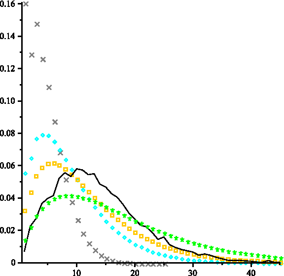
The 5′-3′ limit distance distribution of r-canonical RNA structures and mfe-structures: We display limit distance distribution of r-canonical RNA structures of length 45: (gray cross: r = 1), (cyan diamond: r = 3), (orange square: r = 5), (green star: r = 10) as well as a sample of 10000 mfe-structures obtained from random sequences of length 100 (black line).

Here, a stack of length r is a maximal sequence of “parallel” arcs, \documentclass{aastex}\usepackage{amsbsy}\usepackage{amsfonts}\usepackage{amssymb}\usepackage{bm}\usepackage{mathrsfs}\usepackage{pifont}\usepackage{stmaryrd}\usepackage{textcomp}\usepackage{portland, xspace}\usepackage{amsmath, amsxtra}\pagestyle{empty}\DeclareMathSizes{10}{9}{7}{6}\begin{document}$$( ( i , j ) , ( i + 1 , j - 1 ) , \ldots , ( i + ( r - 1 ) , j - ( r - 1 ) ) )$$\end{document} . RNA secondary structures with stack length ≥ r is called r-canonical RNA secondary structures. Let w_r(n, d) denote the number of r-canonical RNA secondary structures σ_r_,n having distance d_n. We shall write d instead of d_n and consider \documentclass{aastex}\usepackage{amsbsy}\usepackage{amsfonts}\usepackage{amssymb}\usepackage{bm}\usepackage{mathrsfs}\usepackage{pifont}\usepackage{stmaryrd}\usepackage{textcomp}\usepackage{portland, xspace}\usepackage{amsmath, amsxtra}\pagestyle{empty}\DeclareMathSizes{10}{9}{7}{6}\begin{document}\begin{align}{ \bf W}_r ( z , u ) = \sum_{n \geq 0} \sum_{d \geq 0}{ \bf w}_r ( n , d ) \ , z^n u^d , \tag{6.1}\end{align}\end{document}

the bivariate generating function of the number of RNA secondary structure with minimum stack-size r of length n having distance d and set w_r(n) = ∑_d≥0w_r(n, d). Let S_r(z) denote the generating function of r-canonical RNA secondary structures. Set \documentclass{aastex}\usepackage{amsbsy}\usepackage{amsfonts}\usepackage{amssymb}\usepackage{bm}\usepackage{mathrsfs}\usepackage{pifont}\usepackage{stmaryrd}\usepackage{textcomp}\usepackage{portland, xspace}\usepackage{amsmath, amsxtra}\pagestyle{empty}\DeclareMathSizes{10}{9}{7}{6}\begin{document}\begin{align}p_r ( z ) = ( z^{2r} - ( z - 1 ) ( z^{2r} - z^2 + 1 ) ) ^2 - 4z^{2r} ( z^{2r} - z^2 + 1 ) . \tag{6.2}\end{align}\end{document}

Then the generating function of r-canonical secondary structures is given by \documentclass{aastex}\usepackage{amsbsy}\usepackage{amsfonts}\usepackage{amssymb}\usepackage{bm}\usepackage{mathrsfs}\usepackage{pifont}\usepackage{stmaryrd}\usepackage{textcomp}\usepackage{portland, xspace}\usepackage{amsmath, amsxtra}\pagestyle{empty}\DeclareMathSizes{10}{9}{7}{6}\begin{document}\begin{align} { \bf S } _r ( z ) = \frac { ( z^ { 2r } - ( z - 1 ) ( z^ { 2r } - z^2 + 1 ) - \surd { p_r ( z ) } ) } { 2z^ { 2r } } . \tag { 6.3 } \end{align}\end{document}

and we can derive it using symbolic enumeration (Flajolet and Sedgewick, 2009).

Theorem 5

The bivariate generating function of the number of r-canonical RNA secondary structures of length n with distance d, is given by \documentclass{aastex}\usepackage{amsbsy}\usepackage{amsfonts}\usepackage{amssymb}\usepackage{bm}\usepackage{mathrsfs}\usepackage{pifont}\usepackage{stmaryrd}\usepackage{textcomp}\usepackage{portland, xspace}\usepackage{amsmath, amsxtra}\pagestyle{empty}\DeclareMathSizes{10}{9}{7}{6}\begin{document}\begin{align} { \bf W } _r ( z , u ) = \frac { uz^ { 2r } ( { \bf S } _r ( z ) - 1 ) } { ( 1 - zu ) ^2 ( 1 - z^2 + z^ { 2r } ) - ( 1 - zu ) u^2 z^ { 2r } ( { \bf S } _r ( z ) - 1 ) } + \frac { z } { 1 - zu } . \tag { 6.4 } \end{align}\end{document}

Along the lines of our analyis subsequent to Theorem 1, we can then obtain the singular expansion and the limit distributions for the 5′-3′ distances of r-canonical RNA secondary structures (Fig. 9).

Footnotes

Acknowledgments

We are grateful to Thomas J.X. Li for carefully reading the manuscript and special thanks for Fenix W.D. Huang for generating Figure 8 and Emeric Deutsch for pointing out an error in in the discussion.

Disclosure Statement

No competing financial interests exist.

References

Chen

W.Y.C.

, Qin

, Reidys

C.M.

2008. Crossings and nestings of tangled diagrams. Elec. J. Comb., 15:86.

Chen

W.Y.C.

, Deng

E.Y.P.

, Du

R.R.X.

et al. 2007. Crossings and nestings of matchings and partitions. Trans. Am. Math. Soc., 359:1555–1575.

Flajolet

, Fill

J.A.

, Kapur

2005. Singularity analysis, hadamard products, and tree recurrences. J. Comput. Appl. Math., 174:271–313.

Flajolet

, Sedgewick

2009. Analytic Combinatorics. Cambridge University Press: New York.

Fontana

, Konings

D.A.M.

, Stadler

P.F.

1993. Statistics of RNA secondary structures. Biopolymers, 33:1389–1404.

Howell

J.A.

, Smith

T.F.

, Waterman

M.S.

1980. Computation of generating functions for biological molecules. SIAM J. Appl. Math., 39:119–133.

Jin

E.Y.

, Qin

, Reidys

C.M.

2008. Combinatorics of RNA structures with pseudoknots. Bull. Math. Biol, 70:45–67.

Jin

E.Y.

, Reidys

C.M.

2010a. Irreducibility in RNA structures. Bull. Math. Biol., 72:375–399.

Jin

E.Y.

, Reidys

C.M.

2010b. On the decomposition of k-noncrossing RNA structures. Adv. Appl. Math., 44:53–70.

10.

Penner

R.C.

, Waterman

M.S.

1993. Spaces of RNA secondary structures. Adv. Math., 101:31–49.

11.

Reidys

C.M.

2011. Combinatorial Computational Biology of RNA. Springer-Verlag: New York.

12.

Stanley

R.P.

1980. Differentiably finite power series. Eur. J. Comb., 1:175–188.

13.

Waterman

M.S.

1978. Secondary structure of single-stranded nucleic acids. Adv. Math. (Suppl. Studies), 1:167–212.

14.

Waterman

M.S.

1979. Combinatorics of RNA hairpins and cloverleafs. Stud. Appl. Math., 60:91–96.

15.

Waterman

M.S.

, Schmitt

W.R.

1994. Linear trees and RNA secondary structure. Discr. Appl. Math., 51:317–323.

16.

Yoffe

A.M.

, Prinsen

, Gelbart

W.M.

et al. 2011. The ends of a large RNA molecule are necessarily close. Nucleic Acids Res., 39:292–299.

d	1	2	3	4	5	6
p(n, d)	0.161	0.129	0.148	0.126	0.109	0.088
d	7	8	9	10	11	12
p(n, d)	0.069	5.18 × 10⁻²	3.8 × 10⁻²	2.71 × 10⁻²	1.87 × 10⁻²	1.26 × 10⁻²
d	13	14	15	16	17	18
p(n, d)	8.22 × 10⁻³	5.19 × 10⁻³	3.17 × 10⁻³	1.86 × 10⁻³	1.05 × 10⁻³	5.62 × 10⁻⁴
d	19	20	21	22	23	24
p(n, d)	2.85 × 10⁻⁴	1.36 × 10⁻⁴	5.99 × 10⁻⁵	2.41 × 10⁻⁵	8.58 × 10⁻⁶	2.63 × 10⁻⁶
d	25	26	27	28	29
p(n, d)	6.56 × 10⁻⁷	1.24 × 10⁻⁷	1.64 × 10⁻⁸	1.30 × 10⁻⁹	4.65 × 10⁻¹¹