Topology of RNA-RNA Interaction Structures

Abstract

The topological filtration of interacting RNA complexes is studied, and the role is analyzed of certain diagrams called irreducible shadows, which form suitable building blocks for more general structures. We prove that, for two interacting RNAs, called interaction structures, there exist for fixed genus only finitely many irreducible shadows. This implies that, for fixed genus, there are only finitely many classes of interaction structures. In particular, the simplest case of genus zero already provides the formalism for certain types of structures that occur in nature and are not covered by other filtrations. This case of genus zero interaction structures is already of practical interest, is studied here in detail, and is found to be expressed by a multiple context-free grammar that extends the usual one for RNA secondary structures. We show that, in O(n⁶) time and O(n⁴) space complexity, this grammar for genus zero interaction structures provides not only minimum free energy solutions but also the complete partition function and base pairing probabilities.

1. Introduction

RNA-RNA interactions constitute one of the fundamental mechanisms of cellular regulation. For instance, small RNAs binding a larger (m)RNA target include the regulation of translation in both prokaryotes (Narberhaus and Vogel, 2007) and eukaryotes (McManus and Sharp, 2002; Banerjee and Slack, 2002), the targeting of chemical modifications (Bachellerie et al., 2002), insertion editing (Benne, 1992), and transcriptional control (Kugel and Goodrich, 2007). For a variety of RNA classes, including miRNAs, siRNAs, snRNAs, gRNAs, and snoRNAs, a salient feature is the formation of RNA-RNA interaction structures that are far more complex than simple sense-antisense interactions. Accordingly, the ability to predict the details of RNA-RNA interactions in terms of the thermodynamics of binding and in its structural consequences is a necessary prerequisite to understanding RNA-based regulation mechanisms. The exact location of the binding and the subsequent impact of the interaction on the structure of the target molecule has potentially profound biological consequences. In the case of sRNA-mRNA interactions, such details determine whether the sRNA is a positive or negative regulator of transcription depending on whether binding exposes or covers the Shine-Dalgarno sequence (Sharma et al., 2007; Majdalani et al., 2002). Effects along these lines have been observed also using artificially designed opener and closer RNAs that regulate the binding of the HuR protein to human mRNAs (Meisner et al., 2004; Hackermüller et al., 2005).

An RNA molecule is a linearly oriented sequence of four types of nucleotides, namely, A, U, C, and G. This sequence is endowed with a well-defined orientation from the 5′- to the 3′-end and is referred to as the backbone. Each nucleotide can form a base pair by interacting with at most one other nucleotide by establishing hydrogen bonds. Here, we restrict ourselves to Watson-Crick base pairs GC and AU as well as the wobble base pairs GU. In the following, base triples as well as other types of more complex interactions are neglected. RNA structures can be presented as diagrams by drawing the backbone horizontally and all base pairs as arcs in the upper halfplane (Fig. 1). This set of arcs provides our coarse-grained RNA structure, in particular ignoring any spatial embedding or geometry of the molecule beyond its base pairs. Accordingly, particular classes of base pairs translate into specific structure categories, the most prominent of which are secondary structures (Kleitman, 1970; Nussinov et al., 1978; Waterman and Smith, 1978; Waterman, 1979). When represented as diagrams, secondary structures have only non-crossing base pairs (arcs). Beyond RNA secondary structures are the RNA pseudoknot structures that allow for cross serial interactions (Rivas and Eddy, 1999). There are several meaningful filtrations of cross-serial interactions (Orland and Zee, 2002; Reidys et al., 2011, 2010). Given an RNA coarse-grained structure class together with an energy function, “folding” an RNA sequence means to compute a minimum1 free energy configuration (MFE) or a partition function for the sequence.

FIG. 1.

(A) An RNA secondary structure. (B) Its diagram representation.

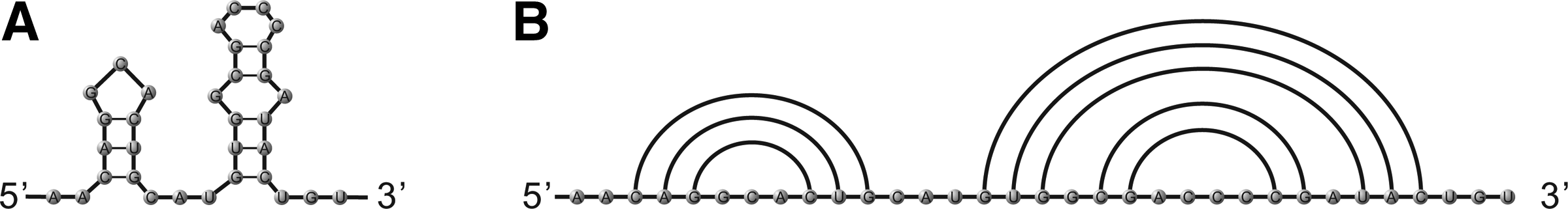
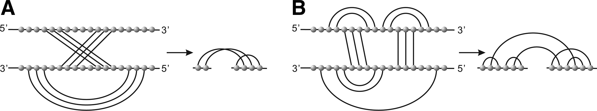
RNA interaction structures are structures over two backbones. We distinguish internal arcs and external arcs as having their endpoints on the same and different backbones, respectively. Interaction structures are represented as two backbones with internal and external arcs drawn in the upper halfplane. Alternatively, they can be represented by drawing the two backbones on top of each other (Fig. 2).

FIG. 2.

(A) Diagram representation of an RNA-RNA interaction structure. (B) The representation of (A) with the two backbones drawn on a horizontal line.

The simplest approach for folding RNA-RNA interaction structures concatenates two (or more) interacting sequences one after another remembering the specific merge point (cut-point) and then employs the standard secondary structure folding algorithm on a single strand with a slightly modified energy model that treats loops containing cut-points as external elements. The software tools RNAcofold (Hofacker et al., 1994; Bernhart et al., 2006), pairfold (Andronescu et al., 2005), and NUPACK (Dirks et al., 2007) subscribe to this strategy. This approach falls short in predicting many important motifs such as kissing-hairpin loops. The paradigm of concatenation has also been generalized to include cross-serial interactions (Rivas and Eddy, 1999). The resulting model, however, still does not generate all relevant interaction structures (Chitsaz et al., 2009b; Qin and Reidys, 2007). An alternative line of thought, implemented in RNAduplex and RNAhybrid (Rehmsmeier et al., 2004), is to neglect all internal base pairings in either strand—i.e., to compute the minimum free energy (MFE) secondary structure of hybridization of otherwise unstructured RNAs. RNAup (Mückstein et al., 2006, 2008) and intaRNA (Busch et al., 2008) restrict interactions to a single interval that remains unpaired in the secondary structure for each partner. As a special case, snoRNA/target complexes are treated more efficiently using a specialized tool (Tafer et al., 2009) due to the highly conserved interaction motif. Algorithmically, the approaches mentioned so far are close relatives of the “classical” RNA folding recursions given by Zuker and Sankoff (1984) and Waterman and Smith (1978). A different approach was taken independently by Pervouchine (2004) and Alkan et al. (2006), who proposed MFE folding algorithms for predicting the AP-structure of two interacting RNA molecules. In this model, the intramolecular structures of each partner are pseudoknot-free, the intermolecular binding pairs are non-crossing, and there is no so-called “zig-zag” motif (see Section 2). The optimal joint structure can be computed in O(N⁶) time and O(N⁴) space by means of dynamic programming.

In contrast to the RNA secondary folding problem, where minimum energy folding and partition functions can be obtained by similar algorithms, the case of interaction structures is more involved. The reason is that simple unambiguous grammars are known for RNA secondary structures (Dowell and Eddy, 2004), while the disambiguation of grammar underlying the Alkan-Pervouchine algorithm requires the introduction of a large number of additional non-terminals (which algorithmically translate into additional dynamic programming tables). The partition function was derived independently by Chitsaz et al. (2009b) (piRNA) and Huang et al. (2009) (rip1). In Huang et al. (2010), probabilities of interaction regions as well as entire hybrid blocks were derived. Although the partition function of joint structures can also be computed in O(N⁶) time and O(N⁴) space, the current implementations require large computational resources. Salari et al. (2009) recently achieved a substantial speed-up making use of the observation that the external interactions mostly occur between pairs of unpaired regions of single structures. Chitsaz et al. (2009a), on the other hand, use tree-structured Markov Random Fields to approximate the joint probability distribution of multiple (≥3) contact regions. The RNA-RNA interaction structures of Huang et al. (2010), Alkan et al. (2006), Hofacker et al. (1994), and Bernhart et al. (2006) have the following features:

• when drawing the two backbones on top of each other, all base pairs are non-crossing, i.e., no pseudoknots formed by internal or external arcs are allowed,

• zig-zag motifs are disallowed.

This article will relax the above constraints and propose a novel filtration of RNA-RNA interaction structures based on the topological fitration of RNA interaction structures. Interaction structures that do not belong to the Alkan-Pervouchine class exist: for instance the integral RNA (hTER) of the human telomerase ribonucleoprotein has a conserved secondary structure that contains a potential pseudoknot (Ly et al., 2003). There is evidence that the two conserved complementary sequences of one stem of the hTER pseudoknot domain can pair intermolecularly in vitro, and that formation of this stem as part of a novel “transpseudoknot” is required for the telomerase to be active in its dimeric form. The classification and expansion of pseudoknotted RNA structures over one backbone via topological genus of the associated fatgraph were first proposed by Orland and Zee (2002), Penner (2004), and Bon et al. (2008)

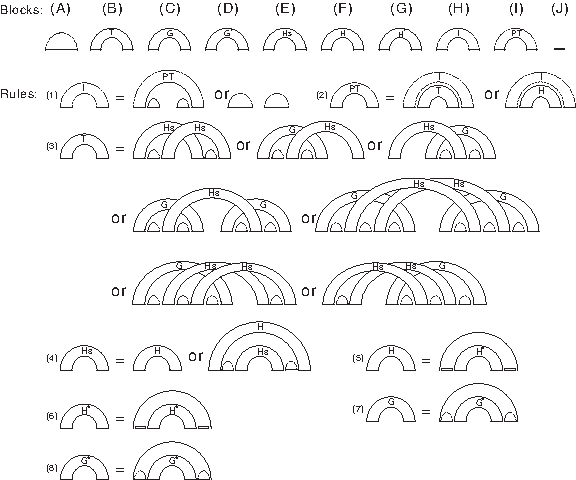
In Reidys et al. (2011) and Zagier (1995), it was proved that, for any genus, there are only finitely many shadows, i.e., particular, simple atomic motifs. In case of genus one, these shadows were first presented in Bon et al. (2008). Shadows give rise to a novel structure class, naturally generalizing RNA secondary structures. These γ-structures (Reidys et al., 2011) are generated by concatenation and nesting of irreducible building blocks of genus ≤γ. We shall present the topological classification of RNA-RNA interaction structures. This filtration gives rise to the notion of γ-structures over two backbones. In analogy to their one-backbone counterparts, γ-structures over two backbones are composed of irreducible building blocks of genus ≤γ and have accordingly arbitrarily high genus. We shall see that, for any fixed genus, there are only finitely many irreducible shadows over two backbones. In particular, we study genus zero structures over two backbones. The latter are the two backbone analogue of RNA secondary structures.2 0-structures over two backbones already exhibit interesting features not shared with AP-structures (Fig. 3). We furthermore derive an unambiguous grammar for 0-structures over two backbones, which translates into an efficient dynamic programming algorithm. This grammar, illustrated in Figure 4, allows the calculation of the minimum free energy, partition function and Boltzmann-sampling. It explicitly treats hybrids and gap structures, i.e., maximal regions with exclusively intermolecular interactions and maximal regions with base pairs over one backbone. The grammar thus facilitates the computation of the probability of hybrids, the target interaction probability between two RNA strands, and the probability of gap structures.

FIG. 3.

(A) Homo sapiens ACA27 snoRNA. This H/ACA box RNA was cloned (Kiss et al., 2004; Ofengand and Bakin, 1997) from a HeLa cell extract immunoprecipitated with an anti-GAR1 antibody. (B) The structure contains two crossing hybrids, which cannot be found in AP-structures.

FIG. 4.

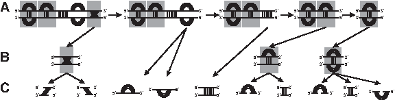
An unambiguous grammar of RNA-RNA interaction structures of genus zero over two backbones. Basic building blocks are: tight structures (gray), secondary structures, and hybrid structures (A). Only tight structures exhibit cross-serial interactions (B) and are further decomposed (C).

2. Basic Facts

2.1. Diagrams

A diagram is a labeled graph over the vertex set \documentclass{aastex}\usepackage{amsbsy}\usepackage{amsfonts}\usepackage{amssymb}\usepackage{bm}\usepackage{mathrsfs}\usepackage{pifont}\usepackage{stmaryrd}\usepackage{textcomp}\usepackage{portland, xspace}\usepackage{amsmath, amsxtra}\pagestyle{empty}\DeclareMathSizes{10}{9}{7}{6}\begin{document} $$[ n ] = \{ 1 , \ldots , n \} $$\end{document} in which each vertex has degree ≤3, represented by drawing its vertices in a horizontal line and its arcs (i, j), where i < j, in the upper half-plane. A backbone is a sequence of consecutive integers contained in [n]. A diagram over b backbones is a diagram together with a partition of [n] into b backbones (Fig. 1B). In the following we shall denote the set of diagrams over one and two backbones by \documentclass{aastex}\usepackage{amsbsy}\usepackage{amsfonts}\usepackage{amssymb}\usepackage{bm}\usepackage{mathrsfs}\usepackage{pifont}\usepackage{stmaryrd}\usepackage{textcomp}\usepackage{portland, xspace}\usepackage{amsmath, amsxtra}\pagestyle{empty}\DeclareMathSizes{10}{9}{7}{6}\begin{document} $${\mathbb D}$$\end{document} and \documentclass{aastex}\usepackage{amsbsy}\usepackage{amsfonts}\usepackage{amssymb}\usepackage{bm}\usepackage{mathrsfs}\usepackage{pifont}\usepackage{stmaryrd}\usepackage{textcomp}\usepackage{portland, xspace}\usepackage{amsmath, amsxtra}\pagestyle{empty}\DeclareMathSizes{10}{9}{7}{6}\begin{document} $${\mathbb E}$$\end{document} , respectively.

The vertices and arcs of a diagram correspond to nucleotides and base pairs, respectively. For a diagram over b backbones, the leftmost vertex of each backbone denotes the 5′ end of the RNA sequence, while the rightmost vertex denotes the 3′ end. In case of b > 1, we shall distinguish two types of arcs: an arc is called exterior if it connects different backbones and interior otherwise. Diagrams over b backbones without exterior arcs are disjoint unions of diagrams over one backbone.

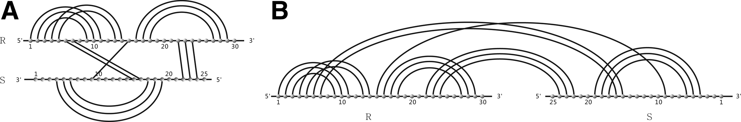
The particular case b = 2 is referred to as RNA interaction structures (Huang et al., 2009, 2010) (Fig. 2A). As mentioned before, interaction structures are oftentimes represented alternatively by drawing the two backbones R and S on top of each other, indexing the vertices R₁ to be the 5′ end of R and S₁ to be the 3′ of S.

A zig-zag is defined as follows: given two sequences R and S, suppose that R_aS_b (i.e., R_a is base paired with S_b), R_iR_j, and \documentclass{aastex}\usepackage{amsbsy}\usepackage{amsfonts}\usepackage{amssymb}\usepackage{bm}\usepackage{mathrsfs}\usepackage{pifont}\usepackage{stmaryrd}\usepackage{textcomp}\usepackage{portland, xspace}\usepackage{amsmath, amsxtra}\pagestyle{empty}\DeclareMathSizes{10}{9}{7}{6}\begin{document} $$S_{i^ \prime}S_{j^ \prime}$$\end{document} with i < a < j and i′ < b < j′. We say that R_i R_j is subsumed in \documentclass{aastex}\usepackage{amsbsy}\usepackage{amsfonts}\usepackage{amssymb}\usepackage{bm}\usepackage{mathrsfs}\usepackage{pifont}\usepackage{stmaryrd}\usepackage{textcomp}\usepackage{portland, xspace}\usepackage{amsmath, amsxtra}\pagestyle{empty}\DeclareMathSizes{10}{9}{7}{6}\begin{document} $$S_{i^ \prime}S_{j^ \prime}$$\end{document} , if for any \documentclass{aastex}\usepackage{amsbsy}\usepackage{amsfonts}\usepackage{amssymb}\usepackage{bm}\usepackage{mathrsfs}\usepackage{pifont}\usepackage{stmaryrd}\usepackage{textcomp}\usepackage{portland, xspace}\usepackage{amsmath, amsxtra}\pagestyle{empty}\DeclareMathSizes{10}{9}{7}{6}\begin{document} $$R_kS_{k^ \prime} \in I$$\end{document} , i < k < j implies i′ < k′ < j′. Finally, a zigzag is a subgraph containing two dependent interior arcs \documentclass{aastex}\usepackage{amsbsy}\usepackage{amsfonts}\usepackage{amssymb}\usepackage{bm}\usepackage{mathrsfs}\usepackage{pifont}\usepackage{stmaryrd}\usepackage{textcomp}\usepackage{portland, xspace}\usepackage{amsmath, amsxtra}\pagestyle{empty}\DeclareMathSizes{10}{9}{7}{6}\begin{document} $$R_{i_1}R_{j_1}$$\end{document} and \documentclass{aastex}\usepackage{amsbsy}\usepackage{amsfonts}\usepackage{amssymb}\usepackage{bm}\usepackage{mathrsfs}\usepackage{pifont}\usepackage{stmaryrd}\usepackage{textcomp}\usepackage{portland, xspace}\usepackage{amsmath, amsxtra}\pagestyle{empty}\DeclareMathSizes{10}{9}{7}{6}\begin{document} $$S_{i_2}S_{j_2}$$\end{document} neither one subsuming the other, (Fig. 5), where dependence here means that there exists at least one exterior arc R_hS_ℓ such that i₁ < h < j₁ and i₂ < ℓ < j₂.

FIG. 5.

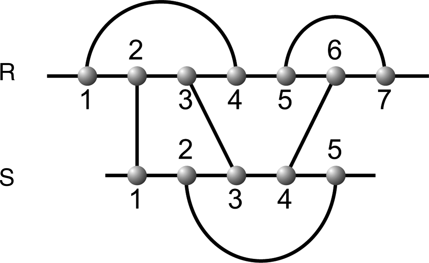
A zig-zag structure. R₁R₄ and S₂S₅ are dependent interior arcs owing to the base pair R₃S₃, but in view of R₂S₁ and R₆S₄, neither subsumes the other.

2.2. From diagrams to topological surfaces

One approach for deriving meaningful filtrations of RNA structure is to pass from diagrams to topological surfaces (Massey, 1967). It is natural to make this transition from combinatorics to topology via fatgraphs (Penner et al., 2010, 2011). A fatgraph \documentclass{aastex}\usepackage{amsbsy}\usepackage{amsfonts}\usepackage{amssymb}\usepackage{bm}\usepackage{mathrsfs}\usepackage{pifont}\usepackage{stmaryrd}\usepackage{textcomp}\usepackage{portland, xspace}\usepackage{amsmath, amsxtra}\pagestyle{empty}\DeclareMathSizes{10}{9}{7}{6}\begin{document} $${\mathbb G}$$\end{document} , sometimes also called “ribbon graph” or “map,” is a graph G together with a collection of cyclic orderings, called a fattening, one such ordering on the half-edges incident on each vertex. Each fatgraph \documentclass{aastex}\usepackage{amsbsy}\usepackage{amsfonts}\usepackage{amssymb}\usepackage{bm}\usepackage{mathrsfs}\usepackage{pifont}\usepackage{stmaryrd}\usepackage{textcomp}\usepackage{portland, xspace}\usepackage{amsmath, amsxtra}\pagestyle{empty}\DeclareMathSizes{10}{9}{7}{6}\begin{document} $${\mathbb G}$$\end{document} determines an oriented surface \documentclass{aastex}\usepackage{amsbsy}\usepackage{amsfonts}\usepackage{amssymb}\usepackage{bm}\usepackage{mathrsfs}\usepackage{pifont}\usepackage{stmaryrd}\usepackage{textcomp}\usepackage{portland, xspace}\usepackage{amsmath, amsxtra}\pagestyle{empty}\DeclareMathSizes{10}{9}{7}{6}\begin{document} $$F ( {\mathbb G} )$$\end{document} as follows: let V (G) be the set of G-vertices and E(G) be the set of G-edges. For each \documentclass{aastex}\usepackage{amsbsy}\usepackage{amsfonts}\usepackage{amssymb}\usepackage{bm}\usepackage{mathrsfs}\usepackage{pifont}\usepackage{stmaryrd}\usepackage{textcomp}\usepackage{portland, xspace}\usepackage{amsmath, amsxtra}\pagestyle{empty}\DeclareMathSizes{10}{9}{7}{6}\begin{document} $$v \in V ( G )$$\end{document} , consider an oriented surface isomorphic to a polygon P_v with 2k sides containing v in its interior where k is the valence of v. The incident edges of v are also incident to a univalent vertex contained in alternating sides of P_v, which are identified with the incident half-edges in the natural way so that the induced counter-clockwise cyclic ordering on the boundary of P_v agrees with the fattening of \documentclass{aastex}\usepackage{amsbsy}\usepackage{amsfonts}\usepackage{amssymb}\usepackage{bm}\usepackage{mathrsfs}\usepackage{pifont}\usepackage{stmaryrd}\usepackage{textcomp}\usepackage{portland, xspace}\usepackage{amsmath, amsxtra}\pagestyle{empty}\DeclareMathSizes{10}{9}{7}{6}\begin{document} $${\mathbb G}$$\end{document} about v. The surface \documentclass{aastex}\usepackage{amsbsy}\usepackage{amsfonts}\usepackage{amssymb}\usepackage{bm}\usepackage{mathrsfs}\usepackage{pifont}\usepackage{stmaryrd}\usepackage{textcomp}\usepackage{portland, xspace}\usepackage{amsmath, amsxtra}\pagestyle{empty}\DeclareMathSizes{10}{9}{7}{6}\begin{document} $$F ( {\mathbb G} )$$\end{document} is the quotient of the disjoint union \documentclass{aastex}\usepackage{amsbsy}\usepackage{amsfonts}\usepackage{amssymb}\usepackage{bm}\usepackage{mathrsfs}\usepackage{pifont}\usepackage{stmaryrd}\usepackage{textcomp}\usepackage{portland, xspace}\usepackage{amsmath, amsxtra}\pagestyle{empty}\DeclareMathSizes{10}{9}{7}{6}\begin{document} $$\sqcup_{v \in V ( G ) }P_v$$\end{document} , where the frontier edges, which are oriented with the polygons on their left, are identified by an orientation-reversing homeomorphism if the corresponding half-edges lie in a common edge of G. This defines the oriented surface \documentclass{aastex}\usepackage{amsbsy}\usepackage{amsfonts}\usepackage{amssymb}\usepackage{bm}\usepackage{mathrsfs}\usepackage{pifont}\usepackage{stmaryrd}\usepackage{textcomp}\usepackage{portland, xspace}\usepackage{amsmath, amsxtra}\pagestyle{empty}\DeclareMathSizes{10}{9}{7}{6}\begin{document} $$F ( {\mathbb G} )$$\end{document} , which is connected if and only if G is and is uniquely determined in this case by its genus g = g(G) ≥ 0 and number r = r(G) ≥ 1 of boundary components. Since \documentclass{aastex}\usepackage{amsbsy}\usepackage{amsfonts}\usepackage{amssymb}\usepackage{bm}\usepackage{mathrsfs}\usepackage{pifont}\usepackage{stmaryrd}\usepackage{textcomp}\usepackage{portland, xspace}\usepackage{amsmath, amsxtra}\pagestyle{empty}\DeclareMathSizes{10}{9}{7}{6}\begin{document} $$F ( {\mathbb G} )$$\end{document} contains G as a deformation retract, they share the Euler characteristic v − e, and the genus of \documentclass{aastex}\usepackage{amsbsy}\usepackage{amsfonts}\usepackage{amssymb}\usepackage{bm}\usepackage{mathrsfs}\usepackage{pifont}\usepackage{stmaryrd}\usepackage{textcomp}\usepackage{portland, xspace}\usepackage{amsmath, amsxtra}\pagestyle{empty}\DeclareMathSizes{10}{9}{7}{6}\begin{document} $$F ( {\mathbb G} )$$\end{document} is given by 2 − 2g − r = v − e.

For an RNA diagram, we may draw a representation as usual so that the backbone is a horizontal line oriented from left to right, and the arcs lie in the upper half-plane. This determines a unique fattening on any diagram; compare the leftmost two panels in Figure 6 for the fatgraph and its corresponding surface. Each boundary component of \documentclass{aastex}\usepackage{amsbsy}\usepackage{amsfonts}\usepackage{amssymb}\usepackage{bm}\usepackage{mathrsfs}\usepackage{pifont}\usepackage{stmaryrd}\usepackage{textcomp}\usepackage{portland, xspace}\usepackage{amsmath, amsxtra}\pagestyle{empty}\DeclareMathSizes{10}{9}{7}{6}\begin{document} $$F ( {\mathbb G} )$$\end{document} determines a closed edge-path or cycle on G, oriented with the surface lying on its left. In particular, a neighborhood of each edge inherits an orientation from that of \documentclass{aastex}\usepackage{amsbsy}\usepackage{amsfonts}\usepackage{amssymb}\usepackage{bm}\usepackage{mathrsfs}\usepackage{pifont}\usepackage{stmaryrd}\usepackage{textcomp}\usepackage{portland, xspace}\usepackage{amsmath, amsxtra}\pagestyle{empty}\DeclareMathSizes{10}{9}{7}{6}\begin{document} $$F ( {\mathbb G} )$$\end{document} which combine to give the oriented cycles as depicted in the third panel of Figure 6. Without affecting topological type of the constructed surface, one may collapse each backbone to a single vertex with the induced fattening called the polygonal model of the RNA, as illustrated in the rightmost panels in Figure 6. It is the orientation of each backbone from the 5′ end to the 3′ end that allows us to transform the fatgraph of an RNA-structure or RNA-interaction into a fatgraph with one or two vertices.

FIG. 6.

(A) The fatgraph of a diagram and its reduction to a single vertex. Contracting the backbone of a diagram into a single vertex decreases the length of the boundary components and preserves the genus. (B) Inflation of edges and vertices to ribbons and discs, as well as walking along the boundary components. Here, we have six vertices, seven edges, and one boundary component. The corresponding surface has Euler characteristic χ = v − e = − 1 and g = 1. At the last step, we collapse each backbone into a single disc again preserving genus. The backbone of the polymer can be recovered by inflating each disk to a backbone segment.

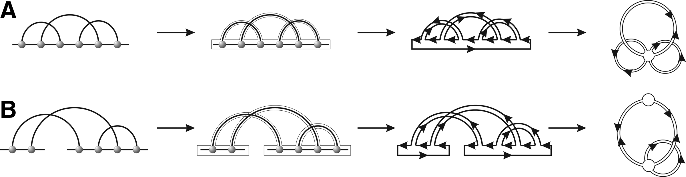
This backbone-collapse preserves orientation, Euler characteristic and genus by construction. It is reversible by inflating each vertex to form a backbone. Using the collapsed fatgraph representation, we see that, for a connected diagram over b backbones, the genus g of the surface (with boundary) is determined by the number n of arcs as well as the number r of boundary components, namely, 2 − 2g − r = v −e = b − n (Fig. 6).

Diagrams over one and two backbones are related by gluing, i.e., we have the mapping \documentclass{aastex}\usepackage{amsbsy}\usepackage{amsfonts}\usepackage{amssymb}\usepackage{bm}\usepackage{mathrsfs}\usepackage{pifont}\usepackage{stmaryrd}\usepackage{textcomp}\usepackage{portland, xspace}\usepackage{amsmath, amsxtra}\pagestyle{empty}\DeclareMathSizes{10}{9}{7}{6}\begin{document}\begin{align*}\alpha :\, {\mathbb E} \rightarrow {\mathbb D} ,\end{align*}\end{document}

where α(E) is obtained by keeping all arcs in E and connecting the 3′ end of R and the 5′ end of S (Fig. 7A).

FIG. 7.

(A) Mapping a diagram over two backbones into a diagram over one backbone by gluing. (B) Mapping from two diagrams over two backbones to a diagram over two backbones by concatenating R₂ after R₁ and S₁ after S₂ preserving the orientation.

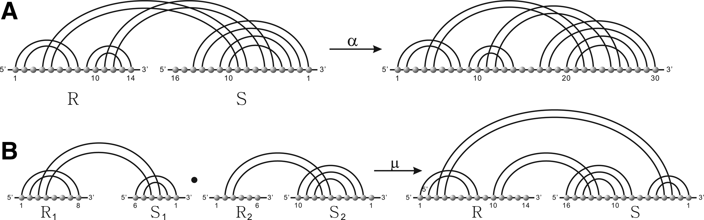
In addition to gluing, there is another operation mapping a pairs of diagram over two backbones into a diagram over two backbones: given two diagrams over two backbones, \documentclass{aastex}\usepackage{amsbsy}\usepackage{amsfonts}\usepackage{amssymb}\usepackage{bm}\usepackage{mathrsfs}\usepackage{pifont}\usepackage{stmaryrd}\usepackage{textcomp}\usepackage{portland, xspace}\usepackage{amsmath, amsxtra}\pagestyle{empty}\DeclareMathSizes{10}{9}{7}{6}\begin{document} $$E_1 , E_2 \in {\mathbb E}$$\end{document} we can insert E₂ into the gap of E₁ by concatenating the backbones R₂ and R₁ and S₁ and S₂ preserving orientation (Fig. 7B). This composition is by construction again a diagram over two backbones denoted E₁•E₂, i.e., we have a mapping \documentclass{aastex}\usepackage{amsbsy}\usepackage{amsfonts}\usepackage{amssymb}\usepackage{bm}\usepackage{mathrsfs}\usepackage{pifont}\usepackage{stmaryrd}\usepackage{textcomp}\usepackage{portland, xspace}\usepackage{amsmath, amsxtra}\pagestyle{empty}\DeclareMathSizes{10}{9}{7}{6}\begin{document}\begin{align*}\mu : \,{\mathbb E} \times {\mathbb E} \longrightarrow {\mathbb E} , \quad \mu ( E_1 , E_2 ) = E_1 \bullet E_2.\end{align*}\end{document}

It is straightforward to see that • is an associative product with unit given by the diagram over two empty backbones. The product • is not commutative.

3. Shadows

Definition 1

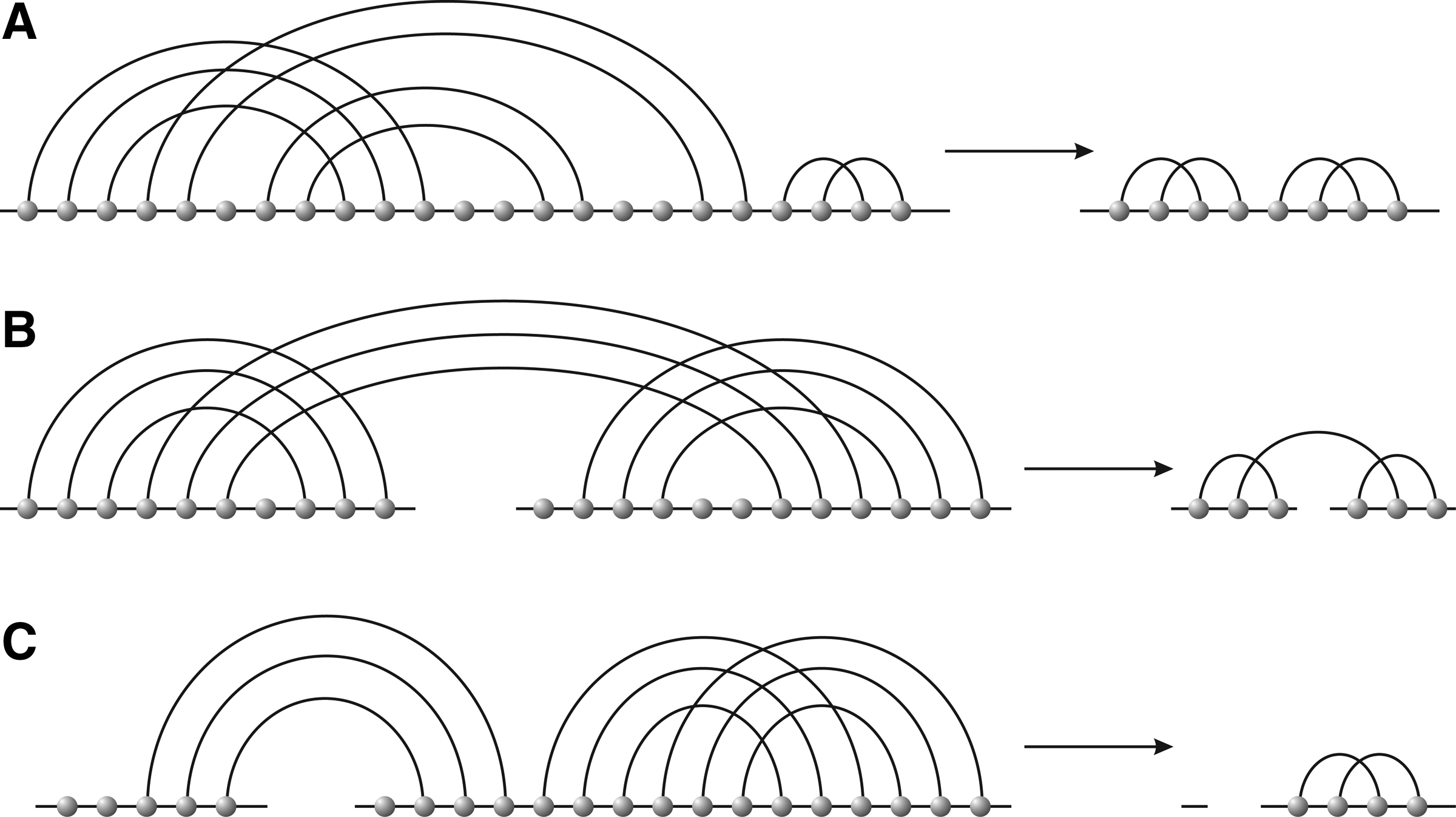
A stack in a diagram is a maximal collection of parallel arcs of the form \documentclass{aastex}\usepackage{amsbsy}\usepackage{amsfonts}\usepackage{amssymb}\usepackage{bm}\usepackage{mathrsfs}\usepackage{pifont}\usepackage{stmaryrd}\usepackage{textcomp}\usepackage{portland, xspace}\usepackage{amsmath, amsxtra}\pagestyle{empty}\DeclareMathSizes{10}{9}{7}{6}\begin{document} $$( i , j ) , ( i + 1 , j - 1 ) , \ldots , ( i + ( \ell - 1 ) , j - ( \ell - 1 ) )$$\end{document} . An arc is non-crossing if there is no other arc in the diagram that crosses it, and a vertex is isolated if it has no arcs incident upon it. A shadow is a diagram with no non-crossing arcs or isolated vertices so that each stack has size one, and a shadow is non-trivial provided each backbone contains at least one paired vertex.

A diagram determines a shadow by removing all non-crossing arcs, deleting all isolated vertices and collapsing each induced stack to a single arc as in Figure 8. We shall denote the shadow of a diagram X by σ(X), so σ²(X) = σ(X). Projecting into the shadow does not affect genus, i.e., g(X) = g(σ(X)). In case there are no crossing arcs, σ(X) becomes an empty diagram on the same number of backbones as X as in Figure 8C). By definition, any empty backbone contributes one boundary component. For example, for a diagram X over b backbones that contains no crossing arcs, σ(X) is a sequence of b empty backbones with b boundary components.

FIG. 8.
Shadows: (A) A diagram over one backbone and its shadow. (B) A diagram over two backbones whose shadow is again over two backbones. (C) A shadow with an empty backbone.

Let us begin by refining an observation about shadows over one backbone from Reidys et al. (2011):

Theorem 1

Shadows of genus g ≥ 1 over one backbone have the following properties:

(a) a shadow of genus g contains at least 2g and at most (6g − 2) arcs; in particular for fixed genus, there are only finitely many shadows;

(b) for any 2g ≤ ℓ ≤ 6g − 2, there exists a shadow of genus g containing exactly ℓ arcs.

Proof

First note that if there is more than one boundary component, then there must be an arc with different boundary components on its two sides and removing this arc decreases r by exactly one while preserving g since the number of arcs is given by n = 2g + r − 1. Furthermore, if there are ν_ℓ boundary components of length ℓ in the polygonal model, then 2n = ∑_ℓℓν_ℓ since each side of each arc is traversed once by the boundary. For a shadow, ν₁ = 0 by definition, and ν₂ ≤ 1 as one sees directly. It therefore follows that 2n = ∑_ℓℓν_ℓ ≥ 3(r − 1) + 2, so 2n = 4g + 2r − 2 ≥ 3r − 1, i.e., 4g − 1 ≥ r. Thus, we have n = 2g + (4g − 1) − 1 = 6g − 2, i.e., any shadow can contain at most 6g − 2 arcs. The lower bound 2g follows directly from n = 2g + r − 1 since r ≥ 1.

Let S_2g be a shadow containing 2g mutually crossing arcs, i.e., each arc crosses any of the remaining (2g − 1) arcs. S_2g has genus g and contains a unique boundary component of length 4g, i.e., traversing 4g non-backbone arcs counted with multiplicity. We construct a new shadow S_2g+1 of genus g containing 2g + 1 arcs, by inserting an arc crossing into S_2g from the 5′ end of S_2g such that the boundary component in S_2g splits into one boundary component of length 3 and another of length 4g + 2 − 3 = 4g − 1. The latter becomes the first boundary component of S_2g+1. The newly inserted arc is by construction crossing, splits a boundary component and preserves genus. We now prove the assertion by induction of the number of inserted arcs. By the induction hypothesis, there exists a shadow S_2g+i of genus g having 2g + i arcs, whose first boundary component has length 4g − i. Again, we insert a crossing arc as described above thereby splitting the first boundary component into one of length 3 and the other of length (4g − (i + 1)). After i = 4g − 2 such insertions, we arrive at a shadow whose first boundary component has length 2 while all other boundary components have length 3. 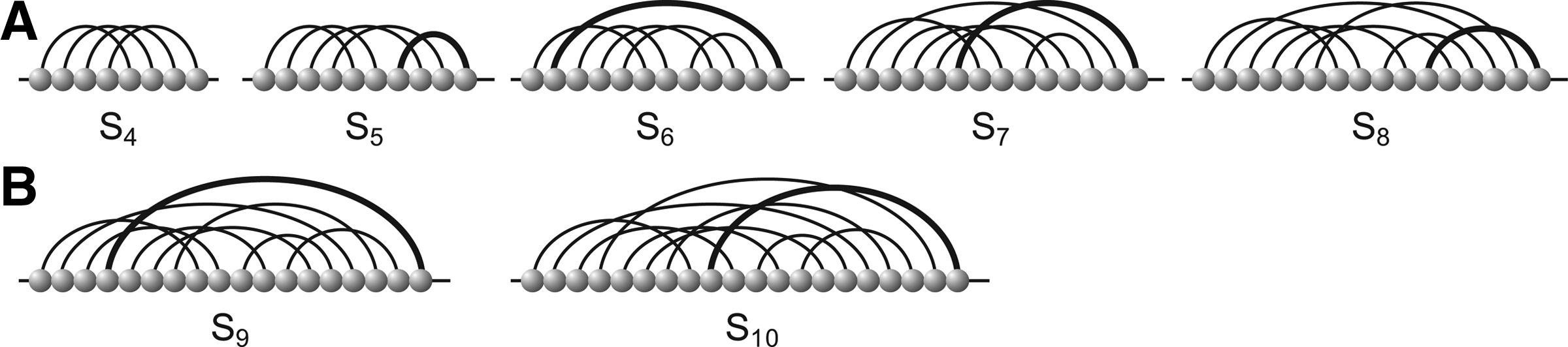Accordingly, there exists a set \documentclass{aastex}\usepackage{amsbsy}\usepackage{amsfonts}\usepackage{amssymb}\usepackage{bm}\usepackage{mathrsfs}\usepackage{pifont}\usepackage{stmaryrd}\usepackage{textcomp}\usepackage{portland, xspace}\usepackage{amsmath, amsxtra}\pagestyle{empty}\DeclareMathSizes{10}{9}{7}{6}\begin{document} $$\{ S_{2g} , S_{2g + 1} , \ldots , S_{2g + ( 4g - 2 ) } \} $$\end{document} of shadows all having genus g, where each S_j contains j arcs (Fig. 9). ■

FIG. 9.
Constructing the sequence of shadows S_ℓ for genus g = 2, see Theorem 1, for 2g = 4 ≤ ℓ ≤ 6g − 2 = 10. Newly inserted arcs are drawn bold.

Corollary 1

A shadow over two backbones has the following properties:

(a) a shadow of genus g ≥ 1 over two backbones contains at least (2g + 1) and at most 6(g + 1) − 2 arcs; a shadow of genus 0 has at least 2 and at most 4 arcs. in particular, the set of such shadows is finite;

(b) for any (2g + 1) ≤ ℓ ≤ 6(g + 1) − 2 in case of g ≥ 1 and 2 ≤ ℓ ≤ 4 in case of g = 0, there exists some shadow over two backbones with genus g containing exactly ℓ arcs.

Proof

We first claim that any shadow of genus g over two backbones can be obtained by cutting the backbone of a shadow over one backbone having either genus g or g + 1. To see this, suppose we are given a shadow of genus g, having r boundary components and n arcs so that 2 − 2g − r = b − n, i.e., g = (2 + n − r − b) / 2, where b = 1. Cutting the backbone then either splits a boundary component or merges two distinct boundary components. Since cutting does not affect arcs and increases the number of backbones by one, we have the resulting genus \documentclass{aastex}\usepackage{amsbsy}\usepackage{amsfonts}\usepackage{amssymb}\usepackage{bm}\usepackage{mathrsfs}\usepackage{pifont}\usepackage{stmaryrd}\usepackage{textcomp}\usepackage{portland, xspace}\usepackage{amsmath, amsxtra}\pagestyle{empty}\DeclareMathSizes{10}{9}{7}{6}\begin{document}\begin{align}g^{ \prime} = ( 2 + n - ( r + 1 ) - ( b + 1 ) ) / 2 = g - 1 \quad {\rm or} \quad g^{ \prime} = ( 2 + n - ( r - 1 ) - ( b + 1 ) ) / 2 = g\end{align}\end{document}

as was claimed. We next observe that a shadow of genus g = 0 over two backbones has at least 2 arcs, while the maximum number of arcs contained in such a shadow is given by 6(0 + 1) − 2 = 4. For g ≥ 1, it is impossible to cut a shadow of genus g having 2g arcs and keep the genus. Thus the shadow of genus g over two backbones has at least 2g + 1 arcs. We can always map an arbitrary shadow over two backbones of genus g via α into a shadow over one backbone, whence the assertion. Theorem 1 guarantees that there are only finitely many such shadows, and the corollary follows. ■

Corollary 2

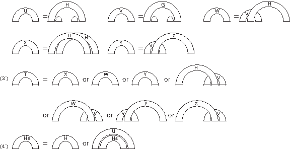
There exist exactly seven non-trivial shadows over two backbones having genus 0.

Proof

There exists no non-trivial shadow over one backbone of genus 0 since 0-structures over one backbone are secondary structures containing exclusively non-crossing arcs. In view of Corollary 1, all non-trivial shadows over two backbones having genus 0 are therefore obtained by cutting the backbone of shadows of genus 1 over one backbone. By inspection, there are seven possible such cuts as in Figure 10. ■

FIG. 10.
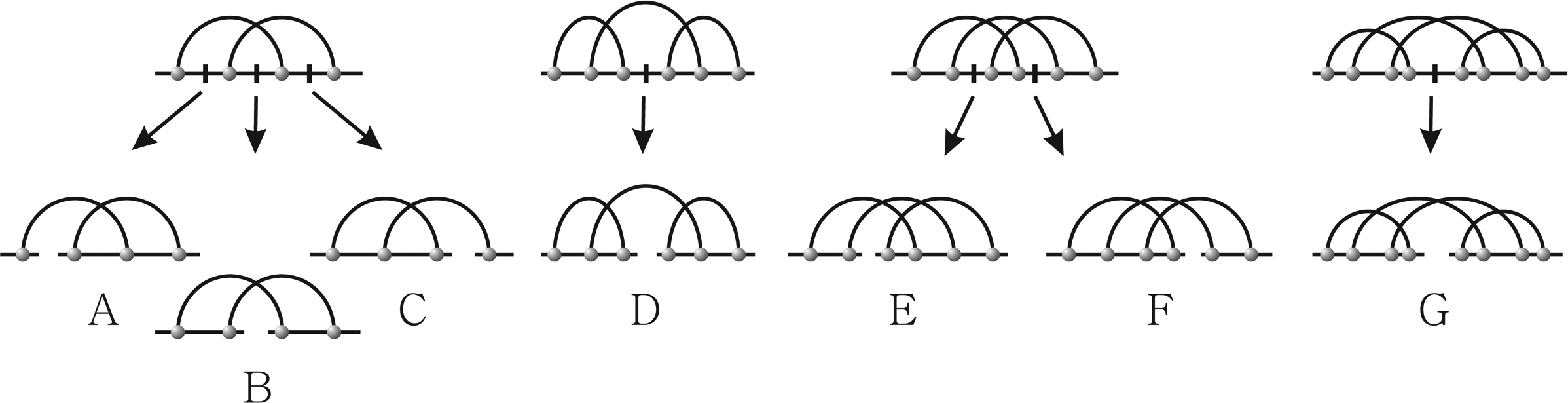
The shadows over two backbones having genus 0 obtained by cutting the four shadows of genus 1 over one backbone.

4. Irreducibility

Definition 2

A diagram E over b backbones is called irreducible if and only if it is connected and for any two arcs, α₁, α_k contained in E, there exists a sequence of arcs \documentclass{aastex}\usepackage{amsbsy}\usepackage{amsfonts}\usepackage{amssymb}\usepackage{bm}\usepackage{mathrsfs}\usepackage{pifont}\usepackage{stmaryrd}\usepackage{textcomp}\usepackage{portland, xspace}\usepackage{amsmath, amsxtra}\pagestyle{empty}\DeclareMathSizes{10}{9}{7}{6}\begin{document} $$( \alpha_1 , \alpha_2 , \ldots , \alpha_{k - 1} , \alpha_k )$$\end{document} such that (α_i, α_i₊₁) are crossing.

We proceed by refining Theorem 1:

Corollary 3

An irreducible shadow having genus g = 0 over two backbones contains at least 2 and at most 4 arcs, and for and 2 ≤ ℓ ≤ 4, there exists an irreducible shadow of genus g = 0 over two backbones having exactly ℓ arcs. An irreducible shadow having genus g ≥ 1 has the following properties:

(a) every irreducible shadow with genus g over two backbones contains at least 2g + 1 and at most 6(g + 1)−2 arcs;

(b) for arbitrary genus g and any 2g + 1 ≤ ℓ ≤ 6g − 2, there exists an irreducible shadow of genus g over one backbone having exactly ℓ arcs.

Proof

Part (a) follows directly from Theorem 1, and for (b), the shadows \documentclass{aastex}\usepackage{amsbsy}\usepackage{amsfonts}\usepackage{amssymb}\usepackage{bm}\usepackage{mathrsfs}\usepackage{pifont}\usepackage{stmaryrd}\usepackage{textcomp}\usepackage{portland, xspace}\usepackage{amsmath, amsxtra}\pagestyle{empty}\DeclareMathSizes{10}{9}{7}{6}\begin{document} $$S_{2g + 1} , \ldots , S_{6g - 2}$$\end{document} generated in the proof of Theorem 1, are in fact irreducible as in Figure 9. ■

Definition 3

Let X be a diagram. We call S′ an irreducible shadow of X (irreducible X-shadow) if and only if S′ is an irreducible shadow and any arc in S′ is contained in X. Let \documentclass{aastex}\usepackage{amsbsy}\usepackage{amsfonts}\usepackage{amssymb}\usepackage{bm}\usepackage{mathrsfs}\usepackage{pifont}\usepackage{stmaryrd}\usepackage{textcomp}\usepackage{portland, xspace}\usepackage{amsmath, amsxtra}\pagestyle{empty}\DeclareMathSizes{10}{9}{7}{6}\begin{document} $${\mathbb I} ( X ) = \{ S^{ \prime} \subset X \mid S^{ \prime}$$\end{document} is an irreducible X-shadow}.

Clearly, our notion of irreducibility recovers for diagrams over one backbone that of Reidys et al. (2011) and Bon et al. (2008). A diagram D over one backbone can iteratively be decomposed by first removing all non-crossing arcs as well as isolated vertices and second by removing irreducible D-shadows iteratively as follows:
• one removes (i.e., cuts the backbone at two points and after removal merges the cut-points) irreducible D-shadows from bottom to top, i.e., such that there exists no irreducible S-shadow that is nested within the one previously removed.

• if the removal of an irreducible D-shadow induces the formation of a non-trivial stack as in Figure 11, then it is collapsed into a single arc.

FIG. 11.
Removing irreducible shadows from “bottom to top.” Any stacks, that are induced by these removals are collapsed into single arcs.

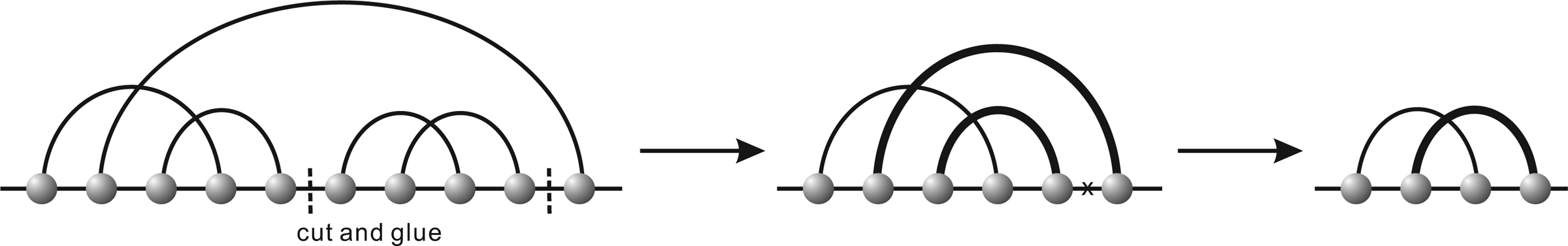
We next extend the decomposition of diagrams over one backbone (Reidys et al., 2011) to diagrams over two backbones. Let E be a diagram over two backbones. By definition, irreducible E-shadows over two backbones are either connected or a disjoint union of two irreducible shadows over one backbone. Thus, E can be decomposed by removing first all non-crossing arcs as well as any isolated vertices and second all irreducible E-shadows in two rounds as follows:
• Remove any irreducible E-shadows over one backbone, from bottom to top, as previously described (Fig. 12).

• Remove the irreducible E-shadows over two backbones iteratively, starting with the irreducible E-shadow containing the leftmost vertex of the second backbone (Fig. 12).

FIG. 12.
Decomposition of a shadow over two backbones. First, from bottom to top, the only irreducible shadow over one backbone is removed. During its removal, a stack of length two is induced (bold arcs), which is projected into a single arc. Second, the two irreducible shadows over two backbones are iteratively removed.

5. γ-Structures Over Two Backbones

Definition 4

A diagram X over b backbones is a γ-structure over b backbones if and only if we have g(S′) ≤ γ for any irreducible X-shadow S′.

With foresight, we refine the notion of irreducible X-shadow as follows: \documentclass{aastex}\usepackage{amsbsy}\usepackage{amsfonts}\usepackage{amssymb}\usepackage{bm}\usepackage{mathrsfs}\usepackage{pifont}\usepackage{stmaryrd}\usepackage{textcomp}\usepackage{portland, xspace}\usepackage{amsmath, amsxtra}\pagestyle{empty}\DeclareMathSizes{10}{9}{7}{6}\begin{document}\begin{align}{\mathbb I}_1 ( E ) & = \{ S^{ \prime} \ \mid \ S^{ \prime} \hbox {is an irreducible} \ E - \hbox{shadow over one backbone} \} , \\ {\mathbb I}_2^{i} ( E ) & = \{ S^{ \prime} \ \mid \ S^{ \prime} \hbox {is an irreducible} \ E - \hbox{shadow over two backbones, } \\ & \ \quad{ \rm where} \ g ( \alpha ( S^{ \prime} ) ) = g ( S^{ \prime} ) + i \} .\end{align}\end{document}

Lemma 1

Suppose E is a γ-structure over two backbones. Then \documentclass{aastex}\usepackage{amsbsy}\usepackage{amsfonts}\usepackage{amssymb}\usepackage{bm}\usepackage{mathrsfs}\usepackage{pifont}\usepackage{stmaryrd}\usepackage{textcomp}\usepackage{portland, xspace}\usepackage{amsmath, amsxtra}\pagestyle{empty}\DeclareMathSizes{10}{9}{7}{6}\begin{document}\begin{align}{g ( E ) = \begin{cases} \displaystyle\sum \limits_{S^{ \prime} \in {\mathbb I}_1 ( E ) } g ( S^{ \prime} ) + \sum \limits_{S^{ \prime} \in {\mathbb I}_2^0 ( E ) } g ( S^{ \prime} ) + \sum \limits_{S^{ \prime} \in {\mathbb I}_2^1 ( E ) } ( g ( S^{ \prime} ) + 1 ) , \ { \rm if} \quad {\mathbb I}_2^0 ( E ) \ne \emptyset; \\ \\ {\displaystyle \sum \limits_{S^{ \prime} \in{\mathbb I}_1 ( E ) } g ( S^{ \prime} ) + \sum \limits_{S^{ \prime} \in {\mathbb I}_2^1 ( E ) } ( g ( S^{ \prime} ) + 1 ) - 1} , \qquad \qquad \quad { \rm if} \quad {\mathbb I}_2^0 ( E ) = \emptyset.\end{cases}} \tag{5.1}\end{align}\end{document}

Proof

By construction, α(E) is a shadow over one backbone consisting of irreducible components of genus at most γ + 1. Thus, α(E) is a (γ + 1)-structure and \documentclass{aastex}\usepackage{amsbsy}\usepackage{amsfonts}\usepackage{amssymb}\usepackage{bm}\usepackage{mathrsfs}\usepackage{pifont}\usepackage{stmaryrd}\usepackage{textcomp}\usepackage{portland, xspace}\usepackage{amsmath, amsxtra}\pagestyle{empty}\DeclareMathSizes{10}{9}{7}{6}\begin{document}\begin{align}g ( \alpha ( E ) ) = \sum_{S^{ \prime} \in {\mathbb I}_1 ( E ) }g ( S^{ \prime} ) + \sum_{S^{ \prime} \in {\mathbb I}_2^0 ( E ) } g ( S^{ \prime} ) + \sum_{S^{ \prime} \in {\mathbb I}_2^1 ( E ) } ( g ( S^{ \prime} ) + 1 ) . \tag{5.2}\end{align}\end{document}

Let \documentclass{aastex}\usepackage{amsbsy}\usepackage{amsfonts}\usepackage{amssymb}\usepackage{bm}\usepackage{mathrsfs}\usepackage{pifont}\usepackage{stmaryrd}\usepackage{textcomp}\usepackage{portland, xspace}\usepackage{amsmath, amsxtra}\pagestyle{empty}\DeclareMathSizes{10}{9}{7}{6}\begin{document} $${\mathbb S}_1 = {\mathbb S}_1 ( E )$$\end{document} be the set of E-subshadows over two backbones where the backbones are on the same boundary component and let \documentclass{aastex}\usepackage{amsbsy}\usepackage{amsfonts}\usepackage{amssymb}\usepackage{bm}\usepackage{mathrsfs}\usepackage{pifont}\usepackage{stmaryrd}\usepackage{textcomp}\usepackage{portland, xspace}\usepackage{amsmath, amsxtra}\pagestyle{empty}\DeclareMathSizes{10}{9}{7}{6}\begin{document} $${\mathbb S}_2 = {\mathbb S}_2 ( E )$$\end{document} be those that are not. We have \documentclass{aastex}\usepackage{amsbsy}\usepackage{amsfonts}\usepackage{amssymb}\usepackage{bm}\usepackage{mathrsfs}\usepackage{pifont}\usepackage{stmaryrd}\usepackage{textcomp}\usepackage{portland, xspace}\usepackage{amsmath, amsxtra}\pagestyle{empty}\DeclareMathSizes{10}{9}{7}{6}\begin{document}\begin{align}g ( S^{ \prime} ) = \begin{cases}g ( \alpha ( S^{ \prime} ) ) , \qquad {\rm iff} \quad S^{ \prime} \in {\mathbb S}_1 ( E ) ; \\ \\ g ( \alpha ( S^{ \prime} ) ) - 1 , \ \ {\rm iff} \quad S^{ \prime} \in {\mathbb S}_2 ( E ) .\end{cases} \tag{5.3}\end{align}\end{document}

Claim 1. Suppose \documentclass{aastex}\usepackage{amsbsy}\usepackage{amsfonts}\usepackage{amssymb}\usepackage{bm}\usepackage{mathrsfs}\usepackage{pifont}\usepackage{stmaryrd}\usepackage{textcomp}\usepackage{portland, xspace}\usepackage{amsmath, amsxtra}\pagestyle{empty}\DeclareMathSizes{10}{9}{7}{6}\begin{document} $${\mathbb I}_2^0 ( E ) = \O$$\end{document} , then \documentclass{aastex}\usepackage{amsbsy}\usepackage{amsfonts}\usepackage{amssymb}\usepackage{bm}\usepackage{mathrsfs}\usepackage{pifont}\usepackage{stmaryrd}\usepackage{textcomp}\usepackage{portland, xspace}\usepackage{amsmath, amsxtra}\pagestyle{empty}\DeclareMathSizes{10}{9}{7}{6}\begin{document}\begin{align}g ( E ) = \sum \limits_{S^{ \prime} \in {\mathbb I}_1 ( E ) } g ( S^{ \prime} ) + \sum \limits_{S^{ \prime} \in {\mathbb I}_2^1 ( E ) } ( g ( S^{ \prime} ) + 1 ) - 1. \tag{5.4}\end{align}\end{document}

To prove this, we use the operation \documentclass{aastex}\usepackage{amsbsy}\usepackage{amsfonts}\usepackage{amssymb}\usepackage{bm}\usepackage{mathrsfs}\usepackage{pifont}\usepackage{stmaryrd}\usepackage{textcomp}\usepackage{portland, xspace}\usepackage{amsmath, amsxtra}\pagestyle{empty}\DeclareMathSizes{10}{9}{7}{6}\begin{document} $$S_1 \bullet S_2 \in {\mathbb S}_2$$\end{document} . By associativity of •, we conclude that E has both backbones on the same boundary component, i.e. \documentclass{aastex}\usepackage{amsbsy}\usepackage{amsfonts}\usepackage{amssymb}\usepackage{bm}\usepackage{mathrsfs}\usepackage{pifont}\usepackage{stmaryrd}\usepackage{textcomp}\usepackage{portland, xspace}\usepackage{amsmath, amsxtra}\pagestyle{empty}\DeclareMathSizes{10}{9}{7}{6}\begin{document}\begin{align}g ( E ) = g ( \alpha ( E ) ) - 1 , \tag{5.5}\end{align}\end{document}

and in view of eq. (5.2), Claim 1 follows.

Claim 2. If \documentclass{aastex}\usepackage{amsbsy}\usepackage{amsfonts}\usepackage{amssymb}\usepackage{bm}\usepackage{mathrsfs}\usepackage{pifont}\usepackage{stmaryrd}\usepackage{textcomp}\usepackage{portland, xspace}\usepackage{amsmath, amsxtra}\pagestyle{empty}\DeclareMathSizes{10}{9}{7}{6}\begin{document} $${\mathbb I}_2^0 ( E ) \neq \O$$\end{document} , then \documentclass{aastex}\usepackage{amsbsy}\usepackage{amsfonts}\usepackage{amssymb}\usepackage{bm}\usepackage{mathrsfs}\usepackage{pifont}\usepackage{stmaryrd}\usepackage{textcomp}\usepackage{portland, xspace}\usepackage{amsmath, amsxtra}\pagestyle{empty}\DeclareMathSizes{10}{9}{7}{6}\begin{document}\begin{align}g (E) = \sum \limits_{S^{\prime} \in {\mathbb I}_1 (E)} g (S^{\prime}) + \sum \limits_{S^{\prime} \in {\mathbb I}_2^1 (E)} (g (S^{\prime}) + 1) + {\sum \limits_{S^{\prime} \in {\mathbb I}_2^0 ( E )} g ( S^{\prime})} \tag{5.6}\end{align}\end{document}

We claim that \documentclass{aastex}\usepackage{amsbsy}\usepackage{amsfonts}\usepackage{amssymb}\usepackage{bm}\usepackage{mathrsfs}\usepackage{pifont}\usepackage{stmaryrd}\usepackage{textcomp}\usepackage{portland, xspace}\usepackage{amsmath, amsxtra}\pagestyle{empty}\DeclareMathSizes{10}{9}{7}{6}\begin{document} $${\mathbb I}_2^0 ( E ) = \O$$\end{document} implies g(E) = g(α(E)). Indeed, \documentclass{aastex}\usepackage{amsbsy}\usepackage{amsfonts}\usepackage{amssymb}\usepackage{bm}\usepackage{mathrsfs}\usepackage{pifont}\usepackage{stmaryrd}\usepackage{textcomp}\usepackage{portland, xspace}\usepackage{amsmath, amsxtra}\pagestyle{empty}\DeclareMathSizes{10}{9}{7}{6}\begin{document} $${\mathbb I}_2^0 ( E ) \ne \O$$\end{document} guarantees that there exists some irreducible shadow \documentclass{aastex}\usepackage{amsbsy}\usepackage{amsfonts}\usepackage{amssymb}\usepackage{bm}\usepackage{mathrsfs}\usepackage{pifont}\usepackage{stmaryrd}\usepackage{textcomp}\usepackage{portland, xspace}\usepackage{amsmath, amsxtra}\pagestyle{empty}\DeclareMathSizes{10}{9}{7}{6}\begin{document} $$S_0^{ \prime} \in {\mathbb I}_2^0 ( E )$$\end{document} . \documentclass{aastex}\usepackage{amsbsy}\usepackage{amsfonts}\usepackage{amssymb}\usepackage{bm}\usepackage{mathrsfs}\usepackage{pifont}\usepackage{stmaryrd}\usepackage{textcomp}\usepackage{portland, xspace}\usepackage{amsmath, amsxtra}\pagestyle{empty}\DeclareMathSizes{10}{9}{7}{6}\begin{document} $$S_0^{ \prime}$$\end{document} has by definition the property \documentclass{aastex}\usepackage{amsbsy}\usepackage{amsfonts}\usepackage{amssymb}\usepackage{bm}\usepackage{mathrsfs}\usepackage{pifont}\usepackage{stmaryrd}\usepackage{textcomp}\usepackage{portland, xspace}\usepackage{amsmath, amsxtra}\pagestyle{empty}\DeclareMathSizes{10}{9}{7}{6}\begin{document} $$g ( \alpha ( S_0^{ \prime} ) ) = g ( S_0^{ \prime} )$$\end{document} , i.e., gluing the two \documentclass{aastex}\usepackage{amsbsy}\usepackage{amsfonts}\usepackage{amssymb}\usepackage{bm}\usepackage{mathrsfs}\usepackage{pifont}\usepackage{stmaryrd}\usepackage{textcomp}\usepackage{portland, xspace}\usepackage{amsmath, amsxtra}\pagestyle{empty}\DeclareMathSizes{10}{9}{7}{6}\begin{document} $$S_0^{ \prime}$$\end{document} -backbones does not merge boundary components, whence \documentclass{aastex}\usepackage{amsbsy}\usepackage{amsfonts}\usepackage{amssymb}\usepackage{bm}\usepackage{mathrsfs}\usepackage{pifont}\usepackage{stmaryrd}\usepackage{textcomp}\usepackage{portland, xspace}\usepackage{amsmath, amsxtra}\pagestyle{empty}\DeclareMathSizes{10}{9}{7}{6}\begin{document} $$S_0^{ \prime} \in {\mathbb S}_1$$\end{document} . Now, at some point \documentclass{aastex}\usepackage{amsbsy}\usepackage{amsfonts}\usepackage{amssymb}\usepackage{bm}\usepackage{mathrsfs}\usepackage{pifont}\usepackage{stmaryrd}\usepackage{textcomp}\usepackage{portland, xspace}\usepackage{amsmath, amsxtra}\pagestyle{empty}\DeclareMathSizes{10}{9}{7}{6}\begin{document} $$S_0^{ \prime}$$\end{document} appears as a factor in the shadow of E which implies \documentclass{aastex}\usepackage{amsbsy}\usepackage{amsfonts}\usepackage{amssymb}\usepackage{bm}\usepackage{mathrsfs}\usepackage{pifont}\usepackage{stmaryrd}\usepackage{textcomp}\usepackage{portland, xspace}\usepackage{amsmath, amsxtra}\pagestyle{empty}\DeclareMathSizes{10}{9}{7}{6}\begin{document} $$E \in {\mathbb S}_1$$\end{document} . Accordingly, we have g(E) = g(α(E)), from which it follows that \documentclass{aastex}\usepackage{amsbsy}\usepackage{amsfonts}\usepackage{amssymb}\usepackage{bm}\usepackage{mathrsfs}\usepackage{pifont}\usepackage{stmaryrd}\usepackage{textcomp}\usepackage{portland, xspace}\usepackage{amsmath, amsxtra}\pagestyle{empty}\DeclareMathSizes{10}{9}{7}{6}\begin{document}\begin{align}g ( E ) = \sum \limits_{S^{ \prime} \in {\mathbb I}_1 ( E ) } g ( S^{ \prime} ) + \sum \limits_{S^{ \prime} \in {\mathbb I}_2^1 ( E ) } ( g ( S^{ \prime} ) + 1 ) + {\sum \limits_{S^{ \prime} \in {\mathbb I}_2^0 ( E )} g ( S^{ \prime})} \tag{5.7}\end{align}\end{document} ■

6. A Grammar For 0-Structures Over Two Backbones

In this section, we develop an unambiguous decomposition grammar \documentclass{aastex}\usepackage{amsbsy}\usepackage{amsfonts}\usepackage{amssymb}\usepackage{bm}\usepackage{mathrsfs}\usepackage{pifont}\usepackage{stmaryrd}\usepackage{textcomp}\usepackage{portland, xspace}\usepackage{amsmath, amsxtra}\pagestyle{empty}\DeclareMathSizes{10}{9}{7}{6}\begin{document} $${ \cal G}_0$$\end{document} for 0-structures over two backbones or 0₂-structures. 0₂-structures map via α into 1-structures over one backbone of genus zero or one. In order to formulate \documentclass{aastex}\usepackage{amsbsy}\usepackage{amsfonts}\usepackage{amssymb}\usepackage{bm}\usepackage{mathrsfs}\usepackage{pifont}\usepackage{stmaryrd}\usepackage{textcomp}\usepackage{portland, xspace}\usepackage{amsmath, amsxtra}\pagestyle{empty}\DeclareMathSizes{10}{9}{7}{6}\begin{document} $${ \cal G}_0$$\end{document} , let us recall that we draw the oriented backbones R and S horizontally and consecutively starting with the 5′ end of R or R₁ and ending with the 3′ end of S or S₁. We denote a structure over two backbones by \documentclass{aastex}\usepackage{amsbsy}\usepackage{amsfonts}\usepackage{amssymb}\usepackage{bm}\usepackage{mathrsfs}\usepackage{pifont}\usepackage{stmaryrd}\usepackage{textcomp}\usepackage{portland, xspace}\usepackage{amsmath, amsxtra}\pagestyle{empty}\DeclareMathSizes{10}{9}{7}{6}\begin{document} $$J^{I}_{i , j;h , \ell} ,$$\end{document} where i, j are vertices contained in R and h, ℓ are contained in S. In particular, we shall write [i, i] for a single vertex letting [i, i − 1] represent an “empty” backbone. For instance, \documentclass{aastex}\usepackage{amsbsy}\usepackage{amsfonts}\usepackage{amssymb}\usepackage{bm}\usepackage{mathrsfs}\usepackage{pifont}\usepackage{stmaryrd}\usepackage{textcomp}\usepackage{portland, xspace}\usepackage{amsmath, amsxtra}\pagestyle{empty}\DeclareMathSizes{10}{9}{7}{6}\begin{document} $$J^I_{i , i - 1;h , \ell}$$\end{document} denotes the structure over one backbone on the interval [h, ℓ] on S, where h ≤ ℓ, \documentclass{aastex}\usepackage{amsbsy}\usepackage{amsfonts}\usepackage{amssymb}\usepackage{bm}\usepackage{mathrsfs}\usepackage{pifont}\usepackage{stmaryrd}\usepackage{textcomp}\usepackage{portland, xspace}\usepackage{amsmath, amsxtra}\pagestyle{empty}\DeclareMathSizes{10}{9}{7}{6}\begin{document} $$J^I_{i , j;h , h - 1}$$\end{document} denotes the structure over one backbone on the interval [i, j] on R, where i ≤ j, and \documentclass{aastex}\usepackage{amsbsy}\usepackage{amsfonts}\usepackage{amssymb}\usepackage{bm}\usepackage{mathrsfs}\usepackage{pifont}\usepackage{stmaryrd}\usepackage{textcomp}\usepackage{portland, xspace}\usepackage{amsmath, amsxtra}\pagestyle{empty}\DeclareMathSizes{10}{9}{7}{6}\begin{document} $$J^I_{i , i - 1 , h , h - 1} = \O$$\end{document} .

The key building blocks of \documentclass{aastex}\usepackage{amsbsy}\usepackage{amsfonts}\usepackage{amssymb}\usepackage{bm}\usepackage{mathrsfs}\usepackage{pifont}\usepackage{stmaryrd}\usepackage{textcomp}\usepackage{portland, xspace}\usepackage{amsmath, amsxtra}\pagestyle{empty}\DeclareMathSizes{10}{9}{7}{6}\begin{document} $${ \cal G}_0$$\end{document} are the following:
• gap-structures: a gap structure \documentclass{aastex}\usepackage{amsbsy}\usepackage{amsfonts}\usepackage{amssymb}\usepackage{bm}\usepackage{mathrsfs}\usepackage{pifont}\usepackage{stmaryrd}\usepackage{textcomp}\usepackage{portland, xspace}\usepackage{amsmath, amsxtra}\pagestyle{empty}\DeclareMathSizes{10}{9}{7}{6}\begin{document} $$J^{G}_{i , j;h , \ell}$$\end{document} is a secondary structure over [i, ℓ] with a gap from j to h such that (i, ℓ) and (j, h) are base pairs; within the two gaps, there are no crossing arcs.

• hybrid-structures: a hybrid structure \documentclass{aastex}\usepackage{amsbsy}\usepackage{amsfonts}\usepackage{amssymb}\usepackage{bm}\usepackage{mathrsfs}\usepackage{pifont}\usepackage{stmaryrd}\usepackage{textcomp}\usepackage{portland, xspace}\usepackage{amsmath, amsxtra}\pagestyle{empty}\DeclareMathSizes{10}{9}{7}{6}\begin{document} $$J^{Hy}_{i_1 , i_ \ell;j_1 , j_ \ell}$$\end{document} is a maximal sequence of intermolecular interior loops consisting of exterior arcs \documentclass{aastex}\usepackage{amsbsy}\usepackage{amsfonts}\usepackage{amssymb}\usepackage{bm}\usepackage{mathrsfs}\usepackage{pifont}\usepackage{stmaryrd}\usepackage{textcomp}\usepackage{portland, xspace}\usepackage{amsmath, amsxtra}\pagestyle{empty}\DeclareMathSizes{10}{9}{7}{6}\begin{document} $$R_{i_1}S_{j_1} , \ldots , R_{i_ \ell}S_{j_ \ell}$$\end{document} where \documentclass{aastex}\usepackage{amsbsy}\usepackage{amsfonts}\usepackage{amssymb}\usepackage{bm}\usepackage{mathrsfs}\usepackage{pifont}\usepackage{stmaryrd}\usepackage{textcomp}\usepackage{portland, xspace}\usepackage{amsmath, amsxtra}\pagestyle{empty}\DeclareMathSizes{10}{9}{7}{6}\begin{document} $$R_{i_h}S_{j_h}$$\end{document} is nested within \documentclass{aastex}\usepackage{amsbsy}\usepackage{amsfonts}\usepackage{amssymb}\usepackage{bm}\usepackage{mathrsfs}\usepackage{pifont}\usepackage{stmaryrd}\usepackage{textcomp}\usepackage{portland, xspace}\usepackage{amsmath, amsxtra}\pagestyle{empty}\DeclareMathSizes{10}{9}{7}{6}\begin{document} $$R_{i_{h + 1}}S_{j_{h + 1}}$$\end{document} and where the internal segments R[i_h + 1, i_h₊₁ − 1] and S[j_h + 1, j_h₊₁ − 1] consist of single-stranded nucleotides only; that is, a hybrid structure (hybrid) is the maximal unbranched stem-loop formed by external arcs.

• tight structures: a tight structure (TS) \documentclass{aastex}\usepackage{amsbsy}\usepackage{amsfonts}\usepackage{amssymb}\usepackage{bm}\usepackage{mathrsfs}\usepackage{pifont}\usepackage{stmaryrd}\usepackage{textcomp}\usepackage{portland, xspace}\usepackage{amsmath, amsxtra}\pagestyle{empty}\DeclareMathSizes{10}{9}{7}{6}\begin{document} $$J^T_{i , j;h , \ell}$$\end{document} is a structure in which the four positions, i, j, h and ℓ are endpoints of an irreducible shadow over two backbones.

• pre-tight structures: a pre-tight structure (PTS) is a structure \documentclass{aastex}\usepackage{amsbsy}\usepackage{amsfonts}\usepackage{amssymb}\usepackage{bm}\usepackage{mathrsfs}\usepackage{pifont}\usepackage{stmaryrd}\usepackage{textcomp}\usepackage{portland, xspace}\usepackage{amsmath, amsxtra}\pagestyle{empty}\DeclareMathSizes{10}{9}{7}{6}\begin{document} $$J^{PT}_{i , j;h , \ell} ,$$\end{document} containing a tight structure \documentclass{aastex}\usepackage{amsbsy}\usepackage{amsfonts}\usepackage{amssymb}\usepackage{bm}\usepackage{mathrsfs}\usepackage{pifont}\usepackage{stmaryrd}\usepackage{textcomp}\usepackage{portland, xspace}\usepackage{amsmath, amsxtra}\pagestyle{empty}\DeclareMathSizes{10}{9}{7}{6}\begin{document} $$J_{i_1 , j;h_1 , \ell}$$\end{document} or a hybrid structure \documentclass{aastex}\usepackage{amsbsy}\usepackage{amsfonts}\usepackage{amssymb}\usepackage{bm}\usepackage{mathrsfs}\usepackage{pifont}\usepackage{stmaryrd}\usepackage{textcomp}\usepackage{portland, xspace}\usepackage{amsmath, amsxtra}\pagestyle{empty}\DeclareMathSizes{10}{9}{7}{6}\begin{document} $$J^{{Hy}_{i_1 , j;h_1 , \ell}}$$\end{document} for some i₁ ≥ i and h₁ ≥ h.

Now we are in position to formulate the production rules of \documentclass{aastex}\usepackage{amsbsy}\usepackage{amsfonts}\usepackage{amssymb}\usepackage{bm}\usepackage{mathrsfs}\usepackage{pifont}\usepackage{stmaryrd}\usepackage{textcomp}\usepackage{portland, xspace}\usepackage{amsmath, amsxtra}\pagestyle{empty}\DeclareMathSizes{10}{9}{7}{6}\begin{document} $${\cal G}_0$$\end{document} , (Fig. 13):
(1) given an arbitrary structure \documentclass{aastex}\usepackage{amsbsy}\usepackage{amsfonts}\usepackage{amssymb}\usepackage{bm}\usepackage{mathrsfs}\usepackage{pifont}\usepackage{stmaryrd}\usepackage{textcomp}\usepackage{portland, xspace}\usepackage{amsmath, amsxtra}\pagestyle{empty}\DeclareMathSizes{10}{9}{7}{6}\begin{document} $$J^I_{i , j;h , \ell} ,$$\end{document} we remove starting from j and ℓ secondary structure blocks until an exterior arc is encountered; such an exterior arc is contained in a pre-tight structure and otherwise, \documentclass{aastex}\usepackage{amsbsy}\usepackage{amsfonts}\usepackage{amssymb}\usepackage{bm}\usepackage{mathrsfs}\usepackage{pifont}\usepackage{stmaryrd}\usepackage{textcomp}\usepackage{portland, xspace}\usepackage{amsmath, amsxtra}\pagestyle{empty}\DeclareMathSizes{10}{9}{7}{6}\begin{document} $$J^I_{i , j;h , \ell}$$\end{document} contains no exterior arc and thus decomposes into two disjoint secondary structures;

(2) the decomposition of pre-tight structures \documentclass{aastex}\usepackage{amsbsy}\usepackage{amsfonts}\usepackage{amssymb}\usepackage{bm}\usepackage{mathrsfs}\usepackage{pifont}\usepackage{stmaryrd}\usepackage{textcomp}\usepackage{portland, xspace}\usepackage{amsmath, amsxtra}\pagestyle{empty}\DeclareMathSizes{10}{9}{7}{6}\begin{document} $$J^{PT}_{i , j;h , \ell}:$$\end{document} if \documentclass{aastex}\usepackage{amsbsy}\usepackage{amsfonts}\usepackage{amssymb}\usepackage{bm}\usepackage{mathrsfs}\usepackage{pifont}\usepackage{stmaryrd}\usepackage{textcomp}\usepackage{portland, xspace}\usepackage{amsmath, amsxtra}\pagestyle{empty}\DeclareMathSizes{10}{9}{7}{6}\begin{document} $$R_jS_{ \ell}$$\end{document} is an exterior arc, then it is decomposed into a hybrid \documentclass{aastex}\usepackage{amsbsy}\usepackage{amsfonts}\usepackage{amssymb}\usepackage{bm}\usepackage{mathrsfs}\usepackage{pifont}\usepackage{stmaryrd}\usepackage{textcomp}\usepackage{portland, xspace}\usepackage{amsmath, amsxtra}\pagestyle{empty}\DeclareMathSizes{10}{9}{7}{6}\begin{document} $$J^{{Hy}}_{i_1 , j;h_1 , \ell}$$\end{document} and an arbitrary substructure \documentclass{aastex}\usepackage{amsbsy}\usepackage{amsfonts}\usepackage{amssymb}\usepackage{bm}\usepackage{mathrsfs}\usepackage{pifont}\usepackage{stmaryrd}\usepackage{textcomp}\usepackage{portland, xspace}\usepackage{amsmath, amsxtra}\pagestyle{empty}\DeclareMathSizes{10}{9}{7}{6}\begin{document} $$J^I_{i , i_1 - 1;h , h_1 - 1}$$\end{document} ; otherwise, it is decomposed into a tight structure \documentclass{aastex}\usepackage{amsbsy}\usepackage{amsfonts}\usepackage{amssymb}\usepackage{bm}\usepackage{mathrsfs}\usepackage{pifont}\usepackage{stmaryrd}\usepackage{textcomp}\usepackage{portland, xspace}\usepackage{amsmath, amsxtra}\pagestyle{empty}\DeclareMathSizes{10}{9}{7}{6}\begin{document} $$J^T_{i_1 , j;h_1 , \ell}$$\end{document} and an arbitrary structure \documentclass{aastex}\usepackage{amsbsy}\usepackage{amsfonts}\usepackage{amssymb}\usepackage{bm}\usepackage{mathrsfs}\usepackage{pifont}\usepackage{stmaryrd}\usepackage{textcomp}\usepackage{portland, xspace}\usepackage{amsmath, amsxtra}\pagestyle{empty}\DeclareMathSizes{10}{9}{7}{6}\begin{document} $$J^I_{i , i_1 - 1;h , h_1 - 1}$$\end{document} ;

(3) in case of tight structures depending on which type of shadow is contained in the tight structure, there are 7 ways to disect into maximal gap structures and hybrid-structures (which in turn collapses into interior and exterior arcs of the irreducible shadow, respectively), as well as secondary structures;

(4) a substructure \documentclass{aastex}\usepackage{amsbsy}\usepackage{amsfonts}\usepackage{amssymb}\usepackage{bm}\usepackage{mathrsfs}\usepackage{pifont}\usepackage{stmaryrd}\usepackage{textcomp}\usepackage{portland, xspace}\usepackage{amsmath, amsxtra}\pagestyle{empty}\DeclareMathSizes{10}{9}{7}{6}\begin{document} $$J^{Hs}_{i , j;h , \ell}$$\end{document} consists of hybrids and secondary structures, where each hybrid structure is maximal.;

(5) a maximal hybrid structure \documentclass{aastex}\usepackage{amsbsy}\usepackage{amsfonts}\usepackage{amssymb}\usepackage{bm}\usepackage{mathrsfs}\usepackage{pifont}\usepackage{stmaryrd}\usepackage{textcomp}\usepackage{portland, xspace}\usepackage{amsmath, amsxtra}\pagestyle{empty}\DeclareMathSizes{10}{9}{7}{6}\begin{document} $$J^{Hy}_{i , j;h , \ell}$$\end{document} is decomposed into an exterior arc R_iS_h and a non-maximal hybrid structure \documentclass{aastex}\usepackage{amsbsy}\usepackage{amsfonts}\usepackage{amssymb}\usepackage{bm}\usepackage{mathrsfs}\usepackage{pifont}\usepackage{stmaryrd}\usepackage{textcomp}\usepackage{portland, xspace}\usepackage{amsmath, amsxtra}\pagestyle{empty}\DeclareMathSizes{10}{9}{7}{6}\begin{document} $$J^{{Hy}^}_{i_1 , j;h_1 , \ell}$$\end{document} with i < i₁ < j* and h < h₁ < ℓ;

(6) a non-maximal hybrid structure \documentclass{aastex}\usepackage{amsbsy}\usepackage{amsfonts}\usepackage{amssymb}\usepackage{bm}\usepackage{mathrsfs}\usepackage{pifont}\usepackage{stmaryrd}\usepackage{textcomp}\usepackage{portland, xspace}\usepackage{amsmath, amsxtra}\pagestyle{empty}\DeclareMathSizes{10}{9}{7}{6}\begin{document} $$J^{{Hy}^}_{i , j;h , \ell}$$\end{document} is decomposed into an exterior arc R_i S_h* and a non-maximal hybrid structure \documentclass{aastex}\usepackage{amsbsy}\usepackage{amsfonts}\usepackage{amssymb}\usepackage{bm}\usepackage{mathrsfs}\usepackage{pifont}\usepackage{stmaryrd}\usepackage{textcomp}\usepackage{portland, xspace}\usepackage{amsmath, amsxtra}\pagestyle{empty}\DeclareMathSizes{10}{9}{7}{6}\begin{document} $$J^{{Hy}^}_{i_1 , j;h_1 , \ell}$$\end{document} with i < i₁ < j* and h < h₁ < ℓ.;

(7) a maximal gap structure \documentclass{aastex}\usepackage{amsbsy}\usepackage{amsfonts}\usepackage{amssymb}\usepackage{bm}\usepackage{mathrsfs}\usepackage{pifont}\usepackage{stmaryrd}\usepackage{textcomp}\usepackage{portland, xspace}\usepackage{amsmath, amsxtra}\pagestyle{empty}\DeclareMathSizes{10}{9}{7}{6}\begin{document} $$J^G_{i , j;h , \ell}$$\end{document} is decomposed via the context-free grammar for secondary structures assuming that there is a virtual hairpin loop in [j, h]; note that the substructure decomposed by a maximal gap structure is no longer maximal; we use \documentclass{aastex}\usepackage{amsbsy}\usepackage{amsfonts}\usepackage{amssymb}\usepackage{bm}\usepackage{mathrsfs}\usepackage{pifont}\usepackage{stmaryrd}\usepackage{textcomp}\usepackage{portland, xspace}\usepackage{amsmath, amsxtra}\pagestyle{empty}\DeclareMathSizes{10}{9}{7}{6}\begin{document} $$J^{G^}_{i , j;h , \ell}$$\end{document} to denote such a non-maximal gap structure derived via this decomposition;

(8) a non-maximal gap structure \documentclass{aastex}\usepackage{amsbsy}\usepackage{amsfonts}\usepackage{amssymb}\usepackage{bm}\usepackage{mathrsfs}\usepackage{pifont}\usepackage{stmaryrd}\usepackage{textcomp}\usepackage{portland, xspace}\usepackage{amsmath, amsxtra}\pagestyle{empty}\DeclareMathSizes{10}{9}{7}{6}\begin{document} $$J^{G^}_{i , j;h , \ell}$$\end{document} is decomposed similarly to the decomposition of a maximal gap structure.

FIG. 13.
The grammar \documentclass{aastex}\usepackage{amsbsy}\usepackage{amsfonts}\usepackage{amssymb}\usepackage{bm}\usepackage{mathrsfs}\usepackage{pifont}\usepackage{stmaryrd}\usepackage{textcomp}\usepackage{portland, xspace}\usepackage{amsmath, amsxtra}\pagestyle{empty}\DeclareMathSizes{10}{9}{7}{6}\begin{document} $${ \cal G}_0$$\end{document} : (A) A secondary structure over [i, j]. (B) A tight structure \documentclass{aastex}\usepackage{amsbsy}\usepackage{amsfonts}\usepackage{amssymb}\usepackage{bm}\usepackage{mathrsfs}\usepackage{pifont}\usepackage{stmaryrd}\usepackage{textcomp}\usepackage{portland, xspace}\usepackage{amsmath, amsxtra}\pagestyle{empty}\DeclareMathSizes{10}{9}{7}{6}\begin{document} $$J^T_{i , j;r , s}$$\end{document} . (C) A gap structure \documentclass{aastex}\usepackage{amsbsy}\usepackage{amsfonts}\usepackage{amssymb}\usepackage{bm}\usepackage{mathrsfs}\usepackage{pifont}\usepackage{stmaryrd}\usepackage{textcomp}\usepackage{portland, xspace}\usepackage{amsmath, amsxtra}\pagestyle{empty}\DeclareMathSizes{10}{9}{7}{6}\begin{document} $$J^G_{i , j;r , s}$$\end{document} over one backbone. (D) A substructure of a gap structure \documentclass{aastex}\usepackage{amsbsy}\usepackage{amsfonts}\usepackage{amssymb}\usepackage{bm}\usepackage{mathrsfs}\usepackage{pifont}\usepackage{stmaryrd}\usepackage{textcomp}\usepackage{portland, xspace}\usepackage{amsmath, amsxtra}\pagestyle{empty}\DeclareMathSizes{10}{9}{7}{6}\begin{document} $$J^{G^}_{i , j;r , s}$$\end{document} such that (i, s) and (j, r) are interior arcs but itself is not a maximal gap structure. (E) A substructure \documentclass{aastex}\usepackage{amsbsy}\usepackage{amsfonts}\usepackage{amssymb}\usepackage{bm}\usepackage{mathrsfs}\usepackage{pifont}\usepackage{stmaryrd}\usepackage{textcomp}\usepackage{portland, xspace}\usepackage{amsmath, amsxtra}\pagestyle{empty}\DeclareMathSizes{10}{9}{7}{6}\begin{document} $$J^{Hs}_{i , j;r , s}$$\end{document} consist of hybrid structures and secondary structures. (F) A hybrid structure \documentclass{aastex}\usepackage{amsbsy}\usepackage{amsfonts}\usepackage{amssymb}\usepackage{bm}\usepackage{mathrsfs}\usepackage{pifont}\usepackage{stmaryrd}\usepackage{textcomp}\usepackage{portland, xspace}\usepackage{amsmath, amsxtra}\pagestyle{empty}\DeclareMathSizes{10}{9}{7}{6}\begin{document} $$J^{Hy}_{i , j;r , s}$$\end{document} . (G) A substructure \documentclass{aastex}\usepackage{amsbsy}\usepackage{amsfonts}\usepackage{amssymb}\usepackage{bm}\usepackage{mathrsfs}\usepackage{pifont}\usepackage{stmaryrd}\usepackage{textcomp}\usepackage{portland, xspace}\usepackage{amsmath, amsxtra}\pagestyle{empty}\DeclareMathSizes{10}{9}{7}{6}\begin{document} $$J^{Hy^}_{i , j;r , s}$$\end{document} of hybrid structure such that (i, j) and (r, s) are exterior arcs but itself is not a hybrid structure because it is not maximum. (H) An arbitrary structure on two backbones. (I) A pre-tight structure \documentclass{aastex}\usepackage{amsbsy}\usepackage{amsfonts}\usepackage{amssymb}\usepackage{bm}\usepackage{mathrsfs}\usepackage{pifont}\usepackage{stmaryrd}\usepackage{textcomp}\usepackage{portland, xspace}\usepackage{amsmath, amsxtra}\pagestyle{empty}\DeclareMathSizes{10}{9}{7}{6}\begin{document} $$J^{PT}_{i , j;r , s}$$\end{document} . (J) An open structure consisting of unpaired bases. (1)–(8) Decomposition rules for the previously defined blocks.

Lemma 2

Any 0-structure over two backbones can uniquely be decomposed via \documentclass{aastex}\usepackage{amsbsy}\usepackage{amsfonts}\usepackage{amssymb}\usepackage{bm}\usepackage{mathrsfs}\usepackage{pifont}\usepackage{stmaryrd}\usepackage{textcomp}\usepackage{portland, xspace}\usepackage{amsmath, amsxtra}\pagestyle{empty}\DeclareMathSizes{10}{9}{7}{6}\begin{document} $${ \cal G}_0$$\end{document} , and any diagram generated by \documentclass{aastex}\usepackage{amsbsy}\usepackage{amsfonts}\usepackage{amssymb}\usepackage{bm}\usepackage{mathrsfs}\usepackage{pifont}\usepackage{stmaryrd}\usepackage{textcomp}\usepackage{portland, xspace}\usepackage{amsmath, amsxtra}\pagestyle{empty}\DeclareMathSizes{10}{9}{7}{6}\begin{document} $${ \cal G}_0$$\end{document} is a 0-structure over two backbones.

Proof

First, we show that a 0₂-structure can uniquely be decomposed into blocks containing exclusively non-crossing arcs. We shall establish this by induction on the number of its irreducible shadows.

Induction basis: any 0₂-structure over two backbones that contains no shadow of genus zero over two backbones exhibits no crossing arcs. Namely, it contains only blocks that are either secondary structures or hybrids. Accordingly, such a structure can be decomposed uniquely via the context-free grammar of secondary structures or the unique decomposition of hybrid-structures.

Induction step: Suppose E_m is a 0₂-structure containing m ≥ 1 irreducible shadows over two backbones of genus 0. We decompose from “inside to outside,” i.e., from the 3′-end of R and the 5′-end of S. Suppose we encounter a substructure S which collapses into an irreducible shadow over two backbones of genus 0. S itself determines a unique maximal tight structure, T_S, such that σ(T_S) = S. Removing T_S from E_m yields a diagram E_m₋₁ over two backbones containing m − 1 irreducible shadows over two backbones of genus 0. The induction hypothesis guarantees the unique decomposition of E_m₋₁ via \documentclass{aastex}\usepackage{amsbsy}\usepackage{amsfonts}\usepackage{amssymb}\usepackage{bm}\usepackage{mathrsfs}\usepackage{pifont}\usepackage{stmaryrd}\usepackage{textcomp}\usepackage{portland, xspace}\usepackage{amsmath, amsxtra}\pagestyle{empty}\DeclareMathSizes{10}{9}{7}{6}\begin{document} $${ \cal G}_0$$\end{document} .

It remains to show how to decompose tight structures: the shadow of a tight structure is by construction irreducible and is given by one of the seven irreducible shadows over two backbones described in Corollary 2. In order to decompose a tight structure, we dissect it into maximal gap structures and hybrid-structures (which in turn collapse into interior and exterior arcs of the irreducible shadow, respectively), as well as secondary structures. All of these elements are \documentclass{aastex}\usepackage{amsbsy}\usepackage{amsfonts}\usepackage{amssymb}\usepackage{bm}\usepackage{mathrsfs}\usepackage{pifont}\usepackage{stmaryrd}\usepackage{textcomp}\usepackage{portland, xspace}\usepackage{amsmath, amsxtra}\pagestyle{empty}\DeclareMathSizes{10}{9}{7}{6}\begin{document} $${ \cal G}_0$$\end{document} -blocks that do not contain any crossing arcs and can therefore be decomposed via a modified version of the context-free grammar of secondary structures, described above. Accordingly, there are seven ways to uniquely decompose a tight structure into blocks containing exclusively non-crossing arcs.

Finally, we show that \documentclass{aastex}\usepackage{amsbsy}\usepackage{amsfonts}\usepackage{amssymb}\usepackage{bm}\usepackage{mathrsfs}\usepackage{pifont}\usepackage{stmaryrd}\usepackage{textcomp}\usepackage{portland, xspace}\usepackage{amsmath, amsxtra}\pagestyle{empty}\DeclareMathSizes{10}{9}{7}{6}\begin{document} $${ \cal G}_0$$\end{document} generates only 0₂-structures. By construction, \documentclass{aastex}\usepackage{amsbsy}\usepackage{amsfonts}\usepackage{amssymb}\usepackage{bm}\usepackage{mathrsfs}\usepackage{pifont}\usepackage{stmaryrd}\usepackage{textcomp}\usepackage{portland, xspace}\usepackage{amsmath, amsxtra}\pagestyle{empty}\DeclareMathSizes{10}{9}{7}{6}\begin{document} $${ \cal G}_0$$\end{document} constructs tight structures via secondary structure blocks, gap-structures and hybrid-structures. It furthermore generates via the insertion of secondary structure blocks, hybrid structures and tight structures. Thus, any structure generated by \documentclass{aastex}\usepackage{amsbsy}\usepackage{amsfonts}\usepackage{amssymb}\usepackage{bm}\usepackage{mathrsfs}\usepackage{pifont}\usepackage{stmaryrd}\usepackage{textcomp}\usepackage{portland, xspace}\usepackage{amsmath, amsxtra}\pagestyle{empty}\DeclareMathSizes{10}{9}{7}{6}\begin{document} $${ \cal G}_0$$\end{document} is a 0₂ -structure, whence the lemma. ■

Theorem 2

The grammar \documentclass{aastex}\usepackage{amsbsy}\usepackage{amsfonts}\usepackage{amssymb}\usepackage{bm}\usepackage{mathrsfs}\usepackage{pifont}\usepackage{stmaryrd}\usepackage{textcomp}\usepackage{portland, xspace}\usepackage{amsmath, amsxtra}\pagestyle{empty}\DeclareMathSizes{10}{9}{7}{6}\begin{document} $${ \cal G}_0$$\end{document} has the following properties:

(a) \documentclass{aastex}\usepackage{amsbsy}\usepackage{amsfonts}\usepackage{amssymb}\usepackage{bm}\usepackage{mathrsfs}\usepackage{pifont}\usepackage{stmaryrd}\usepackage{textcomp}\usepackage{portland, xspace}\usepackage{amsmath, amsxtra}\pagestyle{empty}\DeclareMathSizes{10}{9}{7}{6}\begin{document} $${\cal G}_0$$\end{document} is unambiguous;

(b) \documentclass{aastex}\usepackage{amsbsy}\usepackage{amsfonts}\usepackage{amssymb}\usepackage{bm}\usepackage{mathrsfs}\usepackage{pifont}\usepackage{stmaryrd}\usepackage{textcomp}\usepackage{portland, xspace}\usepackage{amsmath, amsxtra}\pagestyle{empty}\DeclareMathSizes{10}{9}{7}{6}\begin{document} $${\cal G}_0$$\end{document} allows computation of the partition function, base pairing probabilities, the probability of hybrid-blocks, gap-structures and Boltzmann sampling of 0₂-structures,

(c) \documentclass{aastex}\usepackage{amsbsy}\usepackage{amsfonts}\usepackage{amssymb}\usepackage{bm}\usepackage{mathrsfs}\usepackage{pifont}\usepackage{stmaryrd}\usepackage{textcomp}\usepackage{portland, xspace}\usepackage{amsmath, amsxtra}\pagestyle{empty}\DeclareMathSizes{10}{9}{7}{6}\begin{document} $${\cal G}_0$$\end{document} has a time O(n⁶) and space O(n⁴) complexity for generating the partition function of 0₂-structures.

Proof

Assertion (a) follows from Lemma 2. Consequently, \documentclass{aastex}\usepackage{amsbsy}\usepackage{amsfonts}\usepackage{amssymb}\usepackage{bm}\usepackage{mathrsfs}\usepackage{pifont}\usepackage{stmaryrd}\usepackage{textcomp}\usepackage{portland, xspace}\usepackage{amsmath, amsxtra}\pagestyle{empty}\DeclareMathSizes{10}{9}{7}{6}\begin{document}$${\cal G}_0$$\end{document} can be employed to count 0₂-interaction structures over two backbones for given sequences R and S as well as to compute the partition function \documentclass{aastex}\usepackage{amsbsy}\usepackage{amsfonts}\usepackage{amssymb}\usepackage{bm}\usepackage{mathrsfs}\usepackage{pifont}\usepackage{stmaryrd}\usepackage{textcomp}\usepackage{portland, xspace}\usepackage{amsmath, amsxtra}\pagestyle{empty}\DeclareMathSizes{10}{9}{7}{6}\begin{document} \begin{align}Q = \sum_{s \in {\Im_\Re, \mathfrak {s}}} e^{- G (s) \ RT}\end{align} \end{document}

of 0₂-structures, where R is the universal gas constant, T is the temperature, G(s) is energy of structure s over sequence x, and \documentclass{aastex}\usepackage{amsbsy}\usepackage{amsfonts}\usepackage{amssymb}\usepackage{bm}\usepackage{mathrsfs}\usepackage{pifont}\usepackage{stmaryrd}\usepackage{textcomp}\usepackage{portland, xspace}\usepackage{amsmath, amsxtra}\pagestyle{empty}\DeclareMathSizes{10}{9}{7}{6}\begin{document}$$\Im \Re ,\mathfrak{S}$$\end{document} is the set of 0-interaction structures in which all base pairs (i, j) satisfy the base pairing rules for RNA, i.e., \documentclass{aastex}\usepackage{amsbsy}\usepackage{amsfonts}\usepackage{amssymb}\usepackage{bm}\usepackage{mathrsfs}\usepackage{pifont}\usepackage{stmaryrd}\usepackage{textcomp}\usepackage{portland, xspace}\usepackage{amsmath, amsxtra}\pagestyle{empty}\DeclareMathSizes{10}{9}{7}{6}\begin{document} $$( i , j ) \in \{ AU , UA , GC , CG , GU , UG \} $$\end{document} .

As for assertion (b), let N_i_,j;h,ℓ denote the substructure represented by the nonterminal symbol N in \documentclass{aastex}\usepackage{amsbsy}\usepackage{amsfonts}\usepackage{amssymb}\usepackage{bm}\usepackage{mathrsfs}\usepackage{pifont}\usepackage{stmaryrd}\usepackage{textcomp}\usepackage{portland, xspace}\usepackage{amsmath, amsxtra}\pagestyle{empty}\DeclareMathSizes{10}{9}{7}{6}\begin{document} $${ \cal G}_0$$\end{document} over [i, j] and [h, l], where N = {I, PT, T, Hs, Hy, Hy, G, G}. Note that secondary structures are presented by an arbitrary structure I setting one backbone empty. For each of these symbols, we introduce corresponding partial partition functions Q_Ni,j;hℓ. Since \documentclass{aastex}\usepackage{amsbsy}\usepackage{amsfonts}\usepackage{amssymb}\usepackage{bm}\usepackage{mathrsfs}\usepackage{pifont}\usepackage{stmaryrd}\usepackage{textcomp}\usepackage{portland, xspace}\usepackage{amsmath, amsxtra}\pagestyle{empty}\DeclareMathSizes{10}{9}{7}{6}\begin{document} $${ \cal G}_0$$\end{document} is unambiguous, the recursions for the partial partition functions are derived by replacing minima by sums and addition of energy contribution by multiplication of partial partition functions (Voß et al., 2006). For instance, the recursion for the partition functions corresponding to the nonterminal symbol PT reads \documentclass{aastex}\usepackage{amsbsy}\usepackage{amsfonts}\usepackage{amssymb}\usepackage{bm}\usepackage{mathrsfs}\usepackage{pifont}\usepackage{stmaryrd}\usepackage{textcomp}\usepackage{portland, xspace}\usepackage{amsmath, amsxtra}\pagestyle{empty}\DeclareMathSizes{10}{9}{7}{6}\begin{document}\begin{align}Q_{J^{PT}_{i , j;h. \ell}} = \sum \limits_{k_1 , k_2} Q_{J^I_{i , k_1;h , k2 , }} \times Q_{J^T_{k_1 + 1 , j;k_2 + 1; \ell}} + \sum \limits_{k_1 , k_2} Q_{J^I_{i , k_1;h , k2 , }} \times Q_{J^{{Hy}}_{k_1 + 1 , j;k_2 + 1; \ell}}.\end{align}\end{document}

The probabilities \documentclass{aastex}\usepackage{amsbsy}\usepackage{amsfonts}\usepackage{amssymb}\usepackage{bm}\usepackage{mathrsfs}\usepackage{pifont}\usepackage{stmaryrd}\usepackage{textcomp}\usepackage{portland, xspace}\usepackage{amsmath, amsxtra}\pagestyle{empty}\DeclareMathSizes{10}{9}{7}{6}\begin{document} $${\mathbb P}_{N_{i , j;h , \ell}}$$\end{document} of partial substructures of type N are readily calculated from the partial partition functions. These “backward recursions” are analogous to those derived by McCaskill (1990) for secondary structures without crossings. It follows that we have \documentclass{aastex}\usepackage{amsbsy}\usepackage{amsfonts}\usepackage{amssymb}\usepackage{bm}\usepackage{mathrsfs}\usepackage{pifont}\usepackage{stmaryrd}\usepackage{textcomp}\usepackage{portland, xspace}\usepackage{amsmath, amsxtra}\pagestyle{empty}\DeclareMathSizes{10}{9}{7}{6}\begin{document}\begin{align}{\mathbb P}_{N_{i , j}} = \sum {\mathbb P}_s ,\end{align}\end{document}

where the sum is over all 0₂-interaction structures containing N_i_,j;h,ℓ.

Suppose N_i_,j;h,ℓ is obtained by decomposing θ_s. The conditional probabilities \documentclass{aastex}\usepackage{amsbsy}\usepackage{amsfonts}\usepackage{amssymb}\usepackage{bm}\usepackage{mathrsfs}\usepackage{pifont}\usepackage{stmaryrd}\usepackage{textcomp}\usepackage{portland, xspace}\usepackage{amsmath, amsxtra}\pagestyle{empty}\DeclareMathSizes{10}{9}{7}{6}\begin{document} $${\mathbb P}_{N_{i , j;h , \ell} \mid \theta_s}$$\end{document} are then given by \documentclass{aastex}\usepackage{amsbsy}\usepackage{amsfonts}\usepackage{amssymb}\usepackage{bm}\usepackage{mathrsfs}\usepackage{pifont}\usepackage{stmaryrd}\usepackage{textcomp}\usepackage{portland, xspace}\usepackage{amsmath, amsxtra}\pagestyle{empty}\DeclareMathSizes{10}{9}{7}{6}\begin{document} $$Q_{ \theta_s} ( N_{i , j;h , \ell} ) / Q_{ \theta_s}$$\end{document} , where \documentclass{aastex}\usepackage{amsbsy}\usepackage{amsfonts}\usepackage{amssymb}\usepackage{bm}\usepackage{mathrsfs}\usepackage{pifont}\usepackage{stmaryrd}\usepackage{textcomp}\usepackage{portland, xspace}\usepackage{amsmath, amsxtra}\pagestyle{empty}\DeclareMathSizes{10}{9}{7}{6}\begin{document} $$Q_{ \theta_s}$$\end{document} represents the partition function of θ_s and \documentclass{aastex}\usepackage{amsbsy}\usepackage{amsfonts}\usepackage{amssymb}\usepackage{bm}\usepackage{mathrsfs}\usepackage{pifont}\usepackage{stmaryrd}\usepackage{textcomp}\usepackage{portland, xspace}\usepackage{amsmath, amsxtra}\pagestyle{empty}\DeclareMathSizes{10}{9}{7}{6}\begin{document} $$Q_{ \theta_s} ( N_{i , j;h , \ell} )$$\end{document} represents the partition functions for those θ_s-configurations that contain N_i_,j;h,ℓ. Taking the sum over all possible θ_s, we obtain \documentclass{aastex}\usepackage{amsbsy}\usepackage{amsfonts}\usepackage{amssymb}\usepackage{bm}\usepackage{mathrsfs}\usepackage{pifont}\usepackage{stmaryrd}\usepackage{textcomp}\usepackage{portland, xspace}\usepackage{amsmath, amsxtra}\pagestyle{empty}\DeclareMathSizes{10}{9}{7}{6}\begin{document}\begin{align} { \mathbb P } _ { N_ { i , j;h , \ell } } = { \mathbb P } _ { \theta_s } { \frac { Q_ { \theta_s } ( N_ { i , j;h , \ell } ) } { Q_ { \theta_s } } } .\end{align}\end{document}

From this backward recursion, one immediately derives a stochastic backtracing recursion from the probabilities of partial structures that generates a Boltzmann sample of 0-interaction structures; (Tacker et al., 1996; Ding and Lawrence, 2003; Huang et al., 2010). The basic data structure for this sampling is a stack A which stores blocks of the form (i, j; r, s, N), presenting interaction substructures of nonterminal symbols N. L is a set of base pairs storing those removed by the decomposition step in the grammar. We initialize with the block (1, n, I) in A, and L = Ø. In each step, we pick up one element in A and decompose it via the grammar with probability Q^M/Q^N, where Q^N is the partition function of the block which is picked up from A, and Q^M is the partition function of the target block which is decomposed by the rewriting rule. The base pairs which are removed in the decomposition step are moved to L. For instance for the decomposition rule of \documentclass{aastex}\usepackage{amsbsy}\usepackage{amsfonts}\usepackage{amssymb}\usepackage{bm}\usepackage{mathrsfs}\usepackage{pifont}\usepackage{stmaryrd}\usepackage{textcomp}\usepackage{portland, xspace}\usepackage{amsmath, amsxtra}\pagestyle{empty}\DeclareMathSizes{10}{9}{7}{6}\begin{document} $$J^{PT}_{i , j;h , \ell} ,$$\end{document} decomposing block (i, j, PT) into the two blocks: (i, k ₁; h, k₂, I) and (k₁ + 1, j; k₂ + 1, ℓ, T), for fixed indices k₁, k₂, the probability of decomposing (i, j, PT) reads \documentclass{aastex}\usepackage{amsbsy}\usepackage{amsfonts}\usepackage{amssymb}\usepackage{bm}\usepackage{mathrsfs}\usepackage{pifont}\usepackage{stmaryrd}\usepackage{textcomp}\usepackage{portland, xspace}\usepackage{amsmath, amsxtra}\pagestyle{empty}\DeclareMathSizes{10}{9}{7}{6}\begin{document}\begin{align} { \mathbb P } _ { k_1 , k_2 } = { \frac { Q_ { J^I_ { i , k_1;h , k_2 } } \times Q_ { J^ { T } _ { k_1 + 1 , j;k_2 + 1 , \ell } } } { Q_ { J^ { PT } _ { i , j;h , \ell } } } } .\end{align}\end{document}

The sampling step is iterated until A is empty. The resulting 0₂-interaction structure is given by the list L of base pairs. The probability of hybrid-structures can be calculated since a hybrid structure is by construction a block in the grammar, (Huang et al., 2010). The probability of interactions involving a fixed interval [i, j] is given by \documentclass{aastex}\usepackage{amsbsy}\usepackage{amsfonts}\usepackage{amssymb}\usepackage{bm}\usepackage{mathrsfs}\usepackage{pifont}\usepackage{stmaryrd}\usepackage{textcomp}\usepackage{portland, xspace}\usepackage{amsmath, amsxtra}\pagestyle{empty}\DeclareMathSizes{10}{9}{7}{6}\begin{document}\begin{align}{\mathbb P}^{ \rm target}_{ [ i , j ] } = \sum \limits_{h , \ell} {\mathbb P}^{Hy}_{i , j;h. \ell}.\end{align}\end{document}

A gap structure, representing a maximal non-crossing stem on either backbone is also a \documentclass{aastex}\usepackage{amsbsy}\usepackage{amsfonts}\usepackage{amssymb}\usepackage{bm}\usepackage{mathrsfs}\usepackage{pifont}\usepackage{stmaryrd}\usepackage{textcomp}\usepackage{portland, xspace}\usepackage{amsmath, amsxtra}\pagestyle{empty}\DeclareMathSizes{10}{9}{7}{6}\begin{document} $${\cal G}_0$$\end{document} -block, whence its probability is readily computable. Similarly, the probability of parings within the same backbone for a fixed interval [i, j] can be expressed as: \documentclass{aastex}\usepackage{amsbsy}\usepackage{amsfonts}\usepackage{amssymb}\usepackage{bm}\usepackage{mathrsfs}\usepackage{pifont}\usepackage{stmaryrd}\usepackage{textcomp}\usepackage{portland, xspace}\usepackage{amsmath, amsxtra}\pagestyle{empty}\DeclareMathSizes{10}{9}{7}{6}\begin{document}\begin{align}{\mathbb P}^{ \rm paring}_{ [ i , j ] } = \sum \limits_{h , \ell} {\mathbb P}^{G}_{i , j;h. \ell}.\end{align}\end{document}

In order to prove assertion (c), we observe that any product of two blocks has O(n⁶) time complexity. We conclude from this that all \documentclass{aastex}\usepackage{amsbsy}\usepackage{amsfonts}\usepackage{amssymb}\usepackage{bm}\usepackage{mathrsfs}\usepackage{pifont}\usepackage{stmaryrd}\usepackage{textcomp}\usepackage{portland, xspace}\usepackage{amsmath, amsxtra}\pagestyle{empty}\DeclareMathSizes{10}{9}{7}{6}\begin{document} $${ \cal G}_0$$\end{document} -rules, except for (3) and (4) are of O(n⁶) time complexity. It thus remains to analyze (3) and (4).3 To this end, we introduce intermediate blocks whose function is transitional storage.

1. \documentclass{aastex}\usepackage{amsbsy}\usepackage{amsfonts}\usepackage{amssymb}\usepackage{bm}\usepackage{mathrsfs}\usepackage{pifont}\usepackage{stmaryrd}\usepackage{textcomp}\usepackage{portland, xspace}\usepackage{amsmath, amsxtra}\pagestyle{empty}\DeclareMathSizes{10}{9}{7}{6}\begin{document} $$J^U_{i , j;h , \ell}$$\end{document} stores the result of the product \documentclass{aastex}\usepackage{amsbsy}\usepackage{amsfonts}\usepackage{amssymb}\usepackage{bm}\usepackage{mathrsfs}\usepackage{pifont}\usepackage{stmaryrd}\usepackage{textcomp}\usepackage{portland, xspace}\usepackage{amsmath, amsxtra}\pagestyle{empty}\DeclareMathSizes{10}{9}{7}{6}\begin{document} $$J^{{Hy}}_{i , i_1 , h , h_1}$$\end{document} and two secondary structure over interval [i₁ + 1, j] and [h₁ + 1, ℓ] with i ≤ i₁ ≤ j and h ≤ h₁ ≤ ℓ.

2. \documentclass{aastex}\usepackage{amsbsy}\usepackage{amsfonts}\usepackage{amssymb}\usepackage{bm}\usepackage{mathrsfs}\usepackage{pifont}\usepackage{stmaryrd}\usepackage{textcomp}\usepackage{portland, xspace}\usepackage{amsmath, amsxtra}\pagestyle{empty}\DeclareMathSizes{10}{9}{7}{6}\begin{document} $$J^V_{i , j;h , \ell}$$\end{document} stores the result of the product \documentclass{aastex}\usepackage{amsbsy}\usepackage{amsfonts}\usepackage{amssymb}\usepackage{bm}\usepackage{mathrsfs}\usepackage{pifont}\usepackage{stmaryrd}\usepackage{textcomp}\usepackage{portland, xspace}\usepackage{amsmath, amsxtra}\pagestyle{empty}\DeclareMathSizes{10}{9}{7}{6}\begin{document} $$J^G_{i , i_1 ;h_1 , \ell}$$\end{document} and two secondary structure over interval [i₁ + 1, j] and [h + 1, h₁] with i < i₁ ≤ j and h ≤ h₁ < ℓ.

3. \documentclass{aastex}\usepackage{amsbsy}\usepackage{amsfonts}\usepackage{amssymb}\usepackage{bm}\usepackage{mathrsfs}\usepackage{pifont}\usepackage{stmaryrd}\usepackage{textcomp}\usepackage{portland, xspace}\usepackage{amsmath, amsxtra}\pagestyle{empty}\DeclareMathSizes{10}{9}{7}{6}\begin{document} $$J^W_{i , j;h , \ell}$$\end{document} stores the result of the product \documentclass{aastex}\usepackage{amsbsy}\usepackage{amsfonts}\usepackage{amssymb}\usepackage{bm}\usepackage{mathrsfs}\usepackage{pifont}\usepackage{stmaryrd}\usepackage{textcomp}\usepackage{portland, xspace}\usepackage{amsmath, amsxtra}\pagestyle{empty}\DeclareMathSizes{10}{9}{7}{6}\begin{document} $$J^V_{i , i_1 ;\,j_1 , \,j}$$\end{document} and \documentclass{aastex}\usepackage{amsbsy}\usepackage{amsfonts}\usepackage{amssymb}\usepackage{bm}\usepackage{mathrsfs}\usepackage{pifont}\usepackage{stmaryrd}\usepackage{textcomp}\usepackage{portland, xspace}\usepackage{amsmath, amsxtra}\pagestyle{empty}\DeclareMathSizes{10}{9}{7}{6}\begin{document} $$J^{{Hy}}_{i_1 + 1 , j_1 - 1;h , \ell}$$\end{document} with i < i₁ < j₁ < j.

4. \documentclass{aastex}\usepackage{amsbsy}\usepackage{amsfonts}\usepackage{amssymb}\usepackage{bm}\usepackage{mathrsfs}\usepackage{pifont}\usepackage{stmaryrd}\usepackage{textcomp}\usepackage{portland, xspace}\usepackage{amsmath, amsxtra}\pagestyle{empty}\DeclareMathSizes{10}{9}{7}{6}\begin{document} $$J^X_{i , j;h , \ell}$$\end{document} stores the result of the product \documentclass{aastex}\usepackage{amsbsy}\usepackage{amsfonts}\usepackage{amssymb}\usepackage{bm}\usepackage{mathrsfs}\usepackage{pifont}\usepackage{stmaryrd}\usepackage{textcomp}\usepackage{portland, xspace}\usepackage{amsmath, amsxtra}\pagestyle{empty}\DeclareMathSizes{10}{9}{7}{6}\begin{document} $$J^U_{i , i_1 ;h_1 , \ell}$$\end{document} and \documentclass{aastex}\usepackage{amsbsy}\usepackage{amsfonts}\usepackage{amssymb}\usepackage{bm}\usepackage{mathrsfs}\usepackage{pifont}\usepackage{stmaryrd}\usepackage{textcomp}\usepackage{portland, xspace}\usepackage{amsmath, amsxtra}\pagestyle{empty}\DeclareMathSizes{10}{9}{7}{6}\begin{document} $$J^{{Hy}}_{i_1 + 1 , j;h , h_1 - 1}$$\end{document} with i < i₁ < j and h < h₁ < ℓ.

5. \documentclass{aastex}\usepackage{amsbsy}\usepackage{amsfonts}\usepackage{amssymb}\usepackage{bm}\usepackage{mathrsfs}\usepackage{pifont}\usepackage{stmaryrd}\usepackage{textcomp}\usepackage{portland, xspace}\usepackage{amsmath, amsxtra}\pagestyle{empty}\DeclareMathSizes{10}{9}{7}{6}\begin{document} $$J^Y_{i , j;h, \ell}$$\end{document} stores the result of the product \documentclass{aastex}\usepackage{amsbsy}\usepackage{amsfonts}\usepackage{amssymb}\usepackage{bm}\usepackage{mathrsfs}\usepackage{pifont}\usepackage{stmaryrd}\usepackage{textcomp}\usepackage{portland, xspace}\usepackage{amsmath, amsxtra}\pagestyle{empty}\DeclareMathSizes{10}{9}{7}{6}\begin{document} $$J^V_{i , i_1 ;\,j_1 , \,j}$$\end{document} and \documentclass{aastex}\usepackage{amsbsy}\usepackage{amsfonts}\usepackage{amssymb}\usepackage{bm}\usepackage{mathrsfs}\usepackage{pifont}\usepackage{stmaryrd}\usepackage{textcomp}\usepackage{portland, xspace}\usepackage{amsmath, amsxtra}\pagestyle{empty}\DeclareMathSizes{10}{9}{7}{6}\begin{document} $$J^X_{i_1 + 1 , j_1 - 1;h , \ell}$$\end{document} with i < i₁ < j₁ < j.

By virtue of these new blocks, we may rewrite (3) and (4) in terms of (3′) and (4′) as displayed in Figure 14. After including these five intermediate blocks, we obtain two additional, nonterminal symbols in each decomposition rule. Since it requires two free variables to have the product of two nonterminal symbols and at most four variables to describe the two blocks, the decompositions in this form are of O(n⁶) time complexity. We use at most 4-dimensional matrices to store the blocks in \documentclass{aastex}\usepackage{amsbsy}\usepackage{amsfonts}\usepackage{amssymb}\usepackage{bm}\usepackage{mathrsfs}\usepackage{pifont}\usepackage{stmaryrd}\usepackage{textcomp}\usepackage{portland, xspace}\usepackage{amsmath, amsxtra}\pagestyle{empty}\DeclareMathSizes{10}{9}{7}{6}\begin{document} $${ \cal G}_0$$\end{document} , whence the O(n⁴) space complexity. ■

FIG. 14.
The decomposition of \documentclass{aastex}\usepackage{amsbsy}\usepackage{amsfonts}\usepackage{amssymb}\usepackage{bm}\usepackage{mathrsfs}\usepackage{pifont}\usepackage{stmaryrd}\usepackage{textcomp}\usepackage{portland, xspace}\usepackage{amsmath, amsxtra}\pagestyle{empty}\DeclareMathSizes{10}{9}{7}{6}\begin{document} $$J^{T}_{i , j;h , \ell}$$\end{document} and \documentclass{aastex}\usepackage{amsbsy}\usepackage{amsfonts}\usepackage{amssymb}\usepackage{bm}\usepackage{mathrsfs}\usepackage{pifont}\usepackage{stmaryrd}\usepackage{textcomp}\usepackage{portland, xspace}\usepackage{amsmath, amsxtra}\pagestyle{empty}\DeclareMathSizes{10}{9}{7}{6}\begin{document} $$J^{Hs}_{i , j;h , \ell}$$\end{document} via the five intermediate blocks \documentclass{aastex}\usepackage{amsbsy}\usepackage{amsfonts}\usepackage{amssymb}\usepackage{bm}\usepackage{mathrsfs}\usepackage{pifont}\usepackage{stmaryrd}\usepackage{textcomp}\usepackage{portland, xspace}\usepackage{amsmath, amsxtra}\pagestyle{empty}\DeclareMathSizes{10}{9}{7}{6}\begin{document} $$J^{U}_{i , j;h , \ell} ,$$\end{document} \documentclass{aastex}\usepackage{amsbsy}\usepackage{amsfonts}\usepackage{amssymb}\usepackage{bm}\usepackage{mathrsfs}\usepackage{pifont}\usepackage{stmaryrd}\usepackage{textcomp}\usepackage{portland, xspace}\usepackage{amsmath, amsxtra}\pagestyle{empty}\DeclareMathSizes{10}{9}{7}{6}\begin{document} $$J^{V}_{i , j;h , \ell} ,$$\end{document} \documentclass{aastex}\usepackage{amsbsy}\usepackage{amsfonts}\usepackage{amssymb}\usepackage{bm}\usepackage{mathrsfs}\usepackage{pifont}\usepackage{stmaryrd}\usepackage{textcomp}\usepackage{portland, xspace}\usepackage{amsmath, amsxtra}\pagestyle{empty}\DeclareMathSizes{10}{9}{7}{6}\begin{document} $$J^{W}_{i , j;h , \ell} ,$$\end{document} \documentclass{aastex}\usepackage{amsbsy}\usepackage{amsfonts}\usepackage{amssymb}\usepackage{bm}\usepackage{mathrsfs}\usepackage{pifont}\usepackage{stmaryrd}\usepackage{textcomp}\usepackage{portland, xspace}\usepackage{amsmath, amsxtra}\pagestyle{empty}\DeclareMathSizes{10}{9}{7}{6}\begin{document} $$J^{X}_{i , j;h , \ell}$$\end{document} and \documentclass{aastex}\usepackage{amsbsy}\usepackage{amsfonts}\usepackage{amssymb}\usepackage{bm}\usepackage{mathrsfs}\usepackage{pifont}\usepackage{stmaryrd}\usepackage{textcomp}\usepackage{portland, xspace}\usepackage{amsmath, amsxtra}\pagestyle{empty}\DeclareMathSizes{10}{9}{7}{6}\begin{document} $$J^{Y}_{i , j;h , \ell}$$\end{document} . They allow the decomposition of \documentclass{aastex}\usepackage{amsbsy}\usepackage{amsfonts}\usepackage{amssymb}\usepackage{bm}\usepackage{mathrsfs}\usepackage{pifont}\usepackage{stmaryrd}\usepackage{textcomp}\usepackage{portland, xspace}\usepackage{amsmath, amsxtra}\pagestyle{empty}\DeclareMathSizes{10}{9}{7}{6}\begin{document} $$J^{T}_{i , j;h , \ell}$$\end{document} and \documentclass{aastex}\usepackage{amsbsy}\usepackage{amsfonts}\usepackage{amssymb}\usepackage{bm}\usepackage{mathrsfs}\usepackage{pifont}\usepackage{stmaryrd}\usepackage{textcomp}\usepackage{portland, xspace}\usepackage{amsmath, amsxtra}\pagestyle{empty}\DeclareMathSizes{10}{9}{7}{6}\begin{document} $$J^{Hs}_{i , j;h , \ell}$$\end{document} with O(n⁶) time complexity.

7. Discussion

In this article, we have introduced the toplogical filtration of RNA interaction structures and developed the notions of shadows, irreducibility and γ-structures for them. Shadows are of particular importance for the minimum free energy folding since they represent the basic motifs of genus g. Since we have proved that for any genus there are always finitely many such shadows, it is therefore in principle possible to assign them individual energies, which would presumably lead to high specificity.

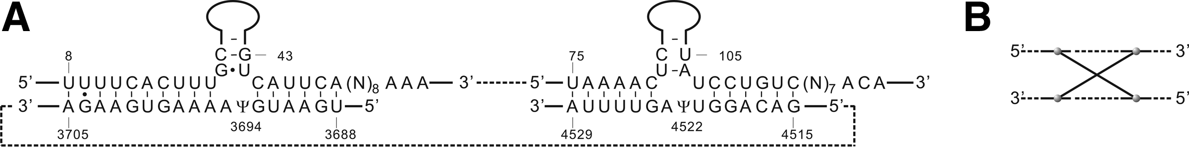
The simplest topological class of RNA interaction structures is that of 0-structures over two backbones. This is the two-backbone analogue of the classical RNA secondary structures. Despite their simple irreducible shadows (Corollary 2), 0-structures over two backbones exhibit features not present in the AP-structures of Pervouchine (2004) and Alkan et al. (2006). Namely, they allow for pseudoknots formed by exterior arcs as reported, for instance, in Homo sapiens ACA27 snoRNA, (Figs. 3 and 15).

FIG. 15.
(A) A 0-structure over two backbones that is not an AP-structure; the crossing hybrid. (B) An AP-structure that is not a 0-structure over two backbones; this structure contains an irreducible shadow over two backbones of genus 1.

Let us next compare AP-structures and 0-structures over two backbones in more detail. Recall that an AP-structure, J(R, S, I), is a graph such that:
1. R, S are secondary structures,

2. I is a set of exterior arcs without external pseudoknots,

3. J(R, S, I) contains no zig-zags.

A tight AP-structure (R(TS)) is a substructure that cannot be decomposed via block decomposition (Huang et al., 2009, 2010). Accordingly, the shadow of a R(TS) is connected and hence irreducibile. R(TS) and tight structures of 0-structures over two backbones are distinct concepts. We have already observed that 0-structures over two backbones are not contained in the set of AP-structures. Likewise, AP-structures are not contained in the set of 0-structures over two backbones, for example, consider a shadow of a 0-structure over two backbones which consist of 3 < x distinct, irreducible shadows over two backbones having genus 0. According to Lemma. 1, the genus of this diagram is x − 1. Drawing an interior arc covering the R-endpoints of these x shadows tightly, the resulting diagram is by construction a R(TS) as in Figure 15. As inserting a single arc changes the genus at most by one, the diagram, R(TS), has genus ≥1, has an irreducible shadow and is consequently not a 0-structure over two backbones.

Footnotes

Disclosure Statement

No competing financial interests exist.

1

with respect to the a priori specified energy function.

2

Which are well-known to be genus zero structures over one backbone.

3

which are in fact O(n¹⁶) for (3) and O(n⁸) for (4) time complexity as it stands.

References

Alkan

, Karakoc

, Nadeau

J.H.

et al. 2006. RNA-RNA interaction prediction and antisense RNA target search. J. Comput. Biol., 13:267–282.

Andronescu

, Zhang

Z.C.

, Condon

2005. Secondary structure prediction of interacting RNA molecules. J. Mol. Biol., 345:1101–1112.

Bachellerie

J.P.

, Cavaillé

, Hüttenhofer

2002. The expanding snoRNA world. Biochimie, 84:775–790.

Banerjee

, Slack

2002. Control of developmental timing by small temporal RNAs: a paradigm for RNA-mediated regulation of gene expression. Bioessays, 24:119–129.

Benne

1992. RNA editing in trypanosomes. the use of guide RNAs. Mol. Biol. Rep., 16:217–227.

Bernhart

, Tafer

, Mückstein

et al. 2006. Partition function and base pairing probabilities of RNA heterodimers. Algorithms Mol. Biol., 1:3.

Bon

, Vernizzi

, Orland

et al. 2008. Topological classification of RNA structures. J. Mol. Biol., 379:900–911.

Busch

, Richter

A.S.

, Backofen

2008. IntaRNA: efficient prediction of bacterial sRNA targets incorporating target site accessibility and seed regions. Bioinformatics, 24:2849–2856.

Chitsaz

, Backofen

, Sahinalp

S.C.

2009a. biRNA: Fast RNA-RNA binding sites prediction. Lect. Notes Comput. Sci., 5724:25–36.

10.

Chitsaz

, Salari

, Sahinalp

S.C.

et al. 2009b. A partition function algorithm for interacting nucleic acid strands. Bioinformatics, 25:i365–i373.

11.

Ding

, Lawrence

C.E.

2003. A statistical sampling algorithm for RNA secondary structure prediction. Nucleic Acids Res., 31:7280–7301.

12.

Dirks

R.M.

, Bois

J.S.

, Schaeffer

J.M.

et al. 2007. Thermodynamic analysis of interacting nucleic acid strands. SIAM Rev., 49:65–88.

13.

Dowell

R.D.

, Eddy

S.R.

2004. Evaluation of several lightweight stochastic context-free grammars for RNA secondary structure prediction. BMC Bioinform., 5:7.

14.

Hackermüller

, Meisner

N.C.

, Auer

et al. 2005. The effect of RNA secondary structures on RNA-ligand binding and the modifier RNA mechanism: a quantitative model. Gene, 345:3–12.

15.

Hofacker

I.L.

, Fontana

, Stadler

P.F.

et al. 1994. Fast folding and comparison of RNA secondary structures. Monatsh. Chem., 125:167–188.

16.

Huang

F.W.D.

, Qin

, Reidys

C.M.

et al. 2009. Partition function and base pairing probabilities for RNA-RNA interaction prediction. Bioinformatics, 25:2646–2654.

17.

Huang

F.W.D.

, Qin

, Reidys

C.M.

et al. 2010. Target prediction and a statistical sampling algorithm for RNA-RNA interaction. Bioinformatics, 26:175–181.

18.

Kiss

A.M.

, Jady

B.E.

, Bertrand

et al. 2004. Human box H/ACA pseudouridylation guide RNA machinery. Mol. Cell. Biol., 24:5797–5807.

19.

Kleitman

1970. Proportions of irreducible diagrams. Stud. Appl. Math., 49:297–299.

20.

Kugel

, Goodrich

2007. An RNA transcriptional regulator templates its own regulatory RNA. Nat. Struct. Mol. Biol., 3:89–90.

21.

, Xu

, Rivera

M.A.

et al. 2003. A role for a novel “trans-pseudoknot” RNA-RNA interaction in the functional dimerization of human telomerase. Genes Dev., 17:1078–1083.

22.

Majdalani

, Hernandez

, Gottesman

2002. Regulation and mode of action of the second small RNA activator of RpoS translation, RprA. Mol. Microbiol., 46:813–826.

23.

Massey

W.S.

1967. Algebraic Topology: An Introduction. Springer-Verlag: New York.

24.

McCaskill

J.S.

1990. The equilibrium partition function and base pair binding probabilities for RNA secondary structure. Biopolymers, 29:1105–1119.

25.

McManus

M.T.

, Sharp

P.A.

2002. Gene silencing in mammals by small interfering RNAs. Nat. Rev., 3:737–747.

26.

Meisner

N.C.

, Hackermüller

, Uhl

et al. 2004. mRNA openers and closers: modulating AU-rich element-controlled mRNA stability by a molecular switch in mRNA secondary structure. Chembiochem., 5:1432–1447.

27.

Mückstein

, Tafer

, Hackermüller

et al. 2006. Thermodynamics of RNA-RNA binding. Bioinformatics, 22:1177–1182.

28.

Mückstein

, Tafer

, Bernhard

S.H.

et al. 2008. Translational control by RNA-RNA interaction: improved computation of RNA-RNA binding thermodynamics. Commun Comput Inf. Sci., 13:114–127.

29.

Narberhaus

, Vogel

2007. Sensory and regulatory RNAs in prokaryotes: a new german research focus. RNA Biol., 4:160–164.

30.

Nussinov

, Pieczenik

G. R.

, Kleitman

D.J.

1978. Algorithms for loop matchings. SIAM J. Appl. Math., 35:68–82.

31.

Ofengand

, Bakin

1997. Mapping to nucleotide resolution of pseudouridine residues in large subunit ribosomal RNAs from representative eukaryotes, prokaryotes, archaebacteria, mitochondria and chloroplasts. J. Mol. Biol., 266:246–268.

32.

Orland

, Zee

2002. RNA folding and large n matrix theory. Nucl. Phys. B, 620:456–476.

33.

Penner

R.C.

2004. Cell decomposition and compactification of Riemann's moduli space in decorated Teichmüller theory, 263–301. Tongring

, Penner

R.C.

Woods Hole Mathematics—Perspectives in Math and Physics. World Scientific: Singapore.

34.

Penner

R.C.

2011. Decorated Teichmüller Theory. European Mathematical Society: Zürich.

35.

Penner

R.C.

, Knudsen

, Wiuf

et al. 2010. Fatgraph models of proteins. Commun. Pure Appl. Math., 63:1249–1297.

36.

Pervouchine

D.D.

2004. IRIS: intermolecular RNA interaction search. Proc. Genome Inform., 15:92–101.

37.

Qin

, Reidys

C. M.

2007. A combinatorial framework for RNA tertiary interaction [Technical Report 0710.3523] arXiv. http://arxiv.org/abs/0710.3523.

38.

Rehmsmeier

, Steffen

, Höchsmann

et al. 2004. Fast and effective prediction of microRNA/target duplexes. Gene, 10:1507–1517.

39.

Reidys

C.M.

et al. 2010. Modular, k-noncrossing diagrams. Electron. J. Comb., 17:R76.

40.

Reidys

C.M.

, Huang

F.W.D.

, Andersen

J.E.

et al. 2011. Topology and prediction of RNA pseudoknots. Bioinformatics, 27:1076–1085.

41.

Rivas

, Eddy

S.R.

1999. A dynamic programming algorithms for RNA structure prediction including pseudoknots. J. Mol. Biol., 285:2053–2068.

42.

Salari

, Backofen

, Sahinalp

S.C.

2009. Fast prediction of RNA-RNA interaction. Lect. Notes Comput. Sci., 5724:261–272.

43.

Sharma

C.M.

, Darfeuille

, Plantinga

T.H.

et al. 2007. A small RNA regulates multiple ABC transporter mRNAs by targeting C/A-rich elements inside and upstream of ribosome-binding sites. Genes Dev., 21:2804–2817.

44.

Tacker

, Stadler

P.F.

, Bornberg-Bauer

E.G.

et al. 1996. Algorithm independent properties of RNA structure prediction. Eur. Biophys. J., 25:115–130.

45.

Tafer

, Kehr

, Hertel

et al. 2010. RNAsnoop: efficient target prediction for box H/ACA snoRNAs. Bioinformatics, 26:610–616.

46.

Voß

, Giegerich

, Rehmsmeier

2006. Complete probabilistic analysis of RNA shapes. BMC Biol., 4:5.

47.

Waterman

M.S.

1979. Combinatorics of RNA hairpins and cloverleaves. Stud. Appl. Math., 60:91–96.

48.

Waterman

M.S.

, Smith

T.F.

1978. RNA secondary structure: a complete mathematical analysis. Math. Biosci., 42:257–266.

49.

Zagier

1995. On the distribution of the number of cycles of elements in symmetric groups. Nieuw Arch. Wisk. IV, 13:489–495.

50.

Zuker

, Sankoff

1984. RNA secondary structures and their prediction. Bull. Math. Biol., 46:591–621.