Combinatorics of the Breakage-Fusion-Bridge Mechanism

Abstract

The breakage-fusion-bridge (BFB) mechanism was proposed over seven decades ago and is a source of genomic variability and gene amplification in cancer. Here we formally model and analyze the BFB mechanism, to our knowledge the first time this has been undertaken. We show that BFB can be modeled as successive inverted prefix duplications of a string. Using this model, we show that BFB can achieve a surprisingly broad range of amplification patterns. We find that a sequence of BFB operations can be found that nearly fits most patterns of copy number increases along a chromosome. We conclude that this limits the usefulness of methods like array CGH for detecting BFB.

1. Introduction

The breakage-fusion-bridge (BFB) mechanism was first proposed by Barbara McClintock in 1938 to explain observations of chromosomes in maize (McClintock, 1938, 1941). BFB begins with a chromosome losing a telomere, perhaps through an unrepaired DNA break or through telomere shortening. As the chromosome replicates, the broken ends of each of its sister chromatids fuse together. During anaphase, as the centromeres of the chromosome migrate to opposite ends of the cell, the fused chromatids are torn apart. Each daughter cell receives a chromosome missing a telomere, and the cycle can begin again (Fig. 1A).

FIG. 1.

The Breakage-Fusion-Bridge (BFB) mechanism. (A) The BFB mechanism is a multiple step process. First, a chromosome loses a telomere (a). Then, the telomere-lacking chromosome (b) replicates. The sister chromatids lacking telomeres fuse together (c). During anaphase, the centromeres separate, forming a dicentric chromosome (d). As the centromeres migrate to opposite ends of the cell, the chromosome is torn apart, and each daughter cell gets a chromosome lacking a telomere (e). (B) After telomere loss (a), sister chromatid fusion (b), and centromere separation (c), the dicentric chromosome may not break in the center of the two centromeres (d). In this case, the break was between the green and cyan segments, so one daughter cell will have a a deletion of those segments while the other will have an inverted duplication. Multiple rounds of inversion and duplication can lead to amplification of chromosomal segments (e).

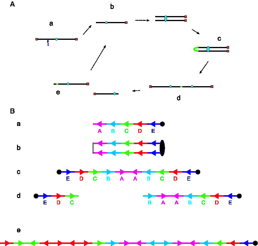
When the fused chromosome is torn apart during anaphase, it likely does not tear exactly in the middle of the two centromeres. As a result, one daughter cell receives a chromosome with a terminal inverted duplication while the other receives a chromosome with a terminal deletion. After many BFB cycles, repeated inverted duplications can result in a dramatic increase in the copy number of segments of the unstable chromosome (Fig. 1B).

BFB's ability to amplify chromosomal segments suggests a role for the mechanism in cancer. Gene amplification is common in tumors. A recent review identified 77 genes whose amplification is implicated in cancer development (Santarius et al., 2010). Multiple lines of evidence indicate that BFB may be responsible for much of this amplification. Telomere dysfunction and crisis is associated with tumorigenesis (Artandi and DePinho, 2010). Such dysfunction is consistent with the initiation and continuation of BFB cycles. Some tumors also display the cytogenetic hallmarks of BFB: chromosomes that stretch across spindle poles during anaphase, dicentric chromosomes, and homogeneously staining regions. Thus, an improved understanding of BFB may shed light on how genomic instability leads to tumor formation and progression.

Observing BFB through classical cytogenetic techniques can be difficult and only provides coarse detail. Recent studies have begun to apply modern methods to the problem of detecting BFB and elucidating its role in generating genomic aberrations. Kitada and Yamasaki performed FISH and array CGH on a lung cancer cell line and showed that the pattern of amplification and rearrangement they observed was consistent with BFB (Kitada and Yamasaki, 2008). Later, Bignell et al. sequenced breakpoints in a breast cancer cell line and confirmed that the copy count and breakpoint patterns on 17q were consistent with a BFB model, purportedly the first demonstration of a sequence-level hallmark of BFB in human cancer (Bignell et al., 2007).

These studies, among others, illustrate the promise of new methods for gaining a more complete understanding of BFB. However, making observations that are consistent with a model does not allow one to conclude that the model is correct. Moreover, without a precise definition of the model under consideration, an investigator cannot use data to refine the model and may succumb to bias when considering evidentiary support for the model.

To address these concerns, we present perhaps the first formal description of the BFB mechanism. We use this formalization to consider the range of amplification patterns that can be produced by BFB. The underlying algorithmic problems are challenging and of unknown complexity. We develop heuristic algorithms and rules to determine if a given pattern is consistent with BFB, based on, among other observations, a tight connection between BFB patterns and trees with certain symmetries. The methods make the problems tractable for practical instances.

Using these methods, we show that BFB-associated amplification patterns are common. In fact, if some imprecision is allowed, a majority of possible patterns are consistent with BFB. This suggests that observing that an amplification pattern could have been produced by BFB is not conclusive evidence that BFB produced the amplification.

2. Formalizing The BFB Schedule

Our first task is to describe a model of the breakage-fusion-bridge mechanism that is both consistent with its biological features and is amenable to computational techniques. We begin by considering a chromosome arm that has lost its telomere. Suppose we label potentially unequally sized intervals along this chromosome arm \documentclass{aastex}\usepackage{amsbsy}\usepackage{amsfonts}\usepackage{amssymb}\usepackage{bm}\usepackage{mathrsfs}\usepackage{pifont}\usepackage{stmaryrd}\usepackage{textcomp}\usepackage{portland, xspace}\usepackage{amsmath, amsxtra}\pagestyle{empty}\DeclareMathSizes{10}{9}{7}{6}\begin{document} $${\rm A} , {\rm B} , {\rm C} , \ldots$$ \end{document} from the telomeric end to the centromere. Then, we trace the fate of these intervals through a BFB cycle.

For illustration, suppose that the chromosome arm, after loss of the telomere, is composed of five intervals, ABCDE. Then, the chromosome is analogous to Figure 1Ba where A,B,C,D,E correspond to the magenta, cyan, green, red, and blue segments, respectively. After replication, fusion, and centromere separation, the whole arm has been duplicated to form a palindrome, EDCBAABCDE, as in Figure 1Bc. This palindromic stretch of DNA is then torn apart. Unless it breaks in the center, between the two A segments, one daughter cell will have a deletion and the other will have an inverted duplication. In Figure 1Bd, one daughter cell gets CDE while the other gets BAABCDE. Thus, BFB cycles can be thought of as operations on a string of chromosomal segments. The only significant restriction this creates is that breaks must occur at segment boundaries, but this is not a loss of generality since the segment boundaries can be defined freely. Moreover, BFB breakpoints may be reused in subsequent BFB cycles (Shimizu et al., 2005), so it is likely useful to keep track of candidate breakpoints.

We are now ready to describe our model. Let Σ (|Σ| = k) be an alphabet where each symbol corresponds to a chromosomal segment, and the ordering of Σ corresponds to the ordering of the segments from telomere to centromere. Let x^t denote the string representing chromosomal segments after t BFB operations. Before any BFB operation, the string is just the initial segments of the chromosome in order. Therefore, x⁰ consists of all k lexicographically ordered characters from Σ. Let x⁻¹ be the reverse of string x, pref(x) be a prefix of the string x, and suff(x) be a suffix of the string x. \documentclass{aastex}\usepackage{amsbsy}\usepackage{amsfonts}\usepackage{amssymb}\usepackage{bm}\usepackage{mathrsfs}\usepackage{pifont}\usepackage{stmaryrd}\usepackage{textcomp}\usepackage{portland, xspace}\usepackage{amsmath, amsxtra}\pagestyle{empty}\DeclareMathSizes{10}{9}{7}{6}\begin{document} \begin{align*} x^t = \begin{cases}{\rm pref} (x^{(t - 1)})^{- 1} x^{(t - 1)} \qquad \hbox{if inverted duplication} \\ \\ {\rm suff} (x^{(t - 1)}) \qquad \qquad \qquad \hbox {if deletion}\end{cases} \tag{1} \end{align*} \end{document}

Define a BFB-schedule as a specific sequence of BFB operations, that is, inverted prefix duplications and prefix deletions. Define x as a BFB(x⁰)-string if it can be generated from x⁰ through a series of BFB operations. For ease of notation, x⁰ is implied, and we refer to x being a BFB-string. The following simple lemmas establish basic properties and ensure that we do not need to worry about deletions.

Lemma 1

Let x be a BFB-string. If x ⁰ is a suffix of x, then x can be obtained from x ⁰ using only inverted prefix duplications.

Proof. Suppose x is produced by a BFB schedule that includes a prefix deletion. The deletion must not delete any characters from the original string x⁰ because if it did, there would be no way to subsequently generate those characters, and x⁰ would not be a suffix of x.

If a prefix deletion removes some of the characters produced by an inverted prefix deletion, then the deletion's affect can be achieved by making the inverted prefix shorter. If the deletion removes all of the characters produced by an inverted prefix deletion, its affect can be achieved by omitting the inverted prefix deletion.

A prefix deletion will remove all or some of the characters produced by at least one previous prefix inverted duplication and all of the characters produced by any duplications after that inverted prefix duplication but before the prefix deletion. If the deletion is removed from the BFB schedule and the appropriate inverted duplications are removed or shortened, then the final string produced will remain the same. ▪

Lemma 2

Suffix Lemma: Any suffix of a BFB-string is itself a BFB-string.

Proof. A suffix of x can be made by a prefix deletion, which is a BFB operation. Since x can be achieved via BFB operations than so can a suffix of x. ▪

3. Algorithms for BFB

We begin with a simple problem: Given string x of length n, determine if x is a BFB-string. This can be solved in O(n) time using the following algorithm:

Algorithm 1
CheckBFB(x)

Input: String x (|x| = n) containing suffix x⁰ (|x⁰| = k)

Output: True if x is a BFB-string

1. (* Find the longest even palindrome beginning at each character in x )

2. for (1 ≤ i < n − k)*

3. \documentclass{aastex}\usepackage{amsbsy}\usepackage{amsfonts}\usepackage{amssymb}\usepackage{bm}\usepackage{mathrsfs}\usepackage{pifont}\usepackage{stmaryrd}\usepackage{textcomp}\usepackage{portland, xspace}\usepackage{amsmath, amsxtra}\pagestyle{empty}\DeclareMathSizes{10}{9}{7}{6}\begin{document} $${\rm P} [{\rm i}] = \max \{\ell \mid x [i \ldots i + 2 \ell] \hbox{\rm is palindromic} \})$$ \end{document}

4. i = 1

5. while (i < n − k)

6. if (P[i] = 0) return false

7. i = i+P[i]

8. return true

Theorem 3

Algorithm CheckBFB checks if x is a BFB-string in O(n) time.

Proof. (Sketch) A string is a BFB-string iff it can be formed by an inverted prefix duplication from another BFB-string or it is the original string, x⁰. An inverted prefix duplication forms an even palindrome at the beginning of a string. CheckBFB finds such a palindrome and then, in effect, recurses on the string that ends at that palindrome's center. Lemma 2 guarantees that that string must be a BFB-string if x is a BFB-string. If a string does not begin with a palindrome, and it is not x⁰, then it is not a BFB-string.

A linear time algorithm for finding maximum palindrome sizes is described in the appendix. The remainder of CheckBFB visits each character at most once, so CheckBFB is in O(n). ▪

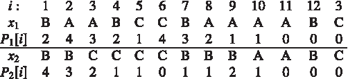
For illustration, consider the palindrome array P₁ for the string x₁ = BAABCCBAAAABC. Starting with i = 1, we can advance i as 1 → 3 → 6 → 10 → 11→ True. For x₂ = BBCCCCBBBAABC, we advance i as 1 → 5 → 6 → False.

Thus, if we are given the full ordering of segments of a chromosome arm, we can determine if BFB could have produced that ordering. However, such complete information is often not available from current technologies. For example, an array CGH or sequencing experiment may only give the count of each segment, not the order. So, we would like to determine if a pattern of copy counts of chromosomal segments could have been produced by BFB. Formally, we define a sequence of positive integer copy counts from telomere to centromere along a chromosome arm as a count-vector ( \documentclass{aastex}\usepackage{amsbsy}\usepackage{amsfonts}\usepackage{amssymb}\usepackage{bm}\usepackage{mathrsfs}\usepackage{pifont}\usepackage{stmaryrd}\usepackage{textcomp}\usepackage{portland, xspace}\usepackage{amsmath, amsxtra}\pagestyle{empty}\DeclareMathSizes{10}{9}{7}{6}\begin{document} $$\vec{n} = [n_1 , n_2 , \ldots , n_k]$$ \end{document} ). We say \documentclass{aastex}\usepackage{amsbsy}\usepackage{amsfonts}\usepackage{amssymb}\usepackage{bm}\usepackage{mathrsfs}\usepackage{pifont}\usepackage{stmaryrd}\usepackage{textcomp}\usepackage{portland, xspace}\usepackage{amsmath, amsxtra}\pagestyle{empty}\DeclareMathSizes{10}{9}{7}{6}\begin{document} $$\vec{n}$$ \end{document} admits a BFB-schedule if there is some BFB-string x whose character counts equal \documentclass{aastex}\usepackage{amsbsy}\usepackage{amsfonts}\usepackage{amssymb}\usepackage{bm}\usepackage{mathrsfs}\usepackage{pifont}\usepackage{stmaryrd}\usepackage{textcomp}\usepackage{portland, xspace}\usepackage{amsmath, amsxtra}\pagestyle{empty}\DeclareMathSizes{10}{9}{7}{6}\begin{document} $$\vec{n}$$ \end{document} . For example, the count vector [6, 3, 5] admits the BFB schedule \documentclass{aastex}\usepackage{amsbsy}\usepackage{amsfonts}\usepackage{amssymb}\usepackage{bm}\usepackage{mathrsfs}\usepackage{pifont}\usepackage{stmaryrd}\usepackage{textcomp}\usepackage{portland, xspace}\usepackage{amsmath, amsxtra}\pagestyle{empty}\DeclareMathSizes{10}{9}{7}{6}\begin{document} \begin{align} \underline{ABC} \rightarrow \underline{C}BAABC \rightarrow \underline{CCBAA}BC \rightarrow \underline{AA}BCCCCBAABC \rightarrow AAAABCCCCBAABC \end{align} \end{document}

In this case, x⁴ has 6, 3, and 5 of characters A, B, and C. We now define our problem:

The BFB-count-vector Problem: Given a count vector \documentclass{aastex}\usepackage{amsbsy}\usepackage{amsfonts}\usepackage{amssymb}\usepackage{bm}\usepackage{mathrsfs}\usepackage{pifont}\usepackage{stmaryrd}\usepackage{textcomp}\usepackage{portland, xspace}\usepackage{amsmath, amsxtra}\pagestyle{empty}\DeclareMathSizes{10}{9}{7}{6}\begin{document} $$\vec{n}$$ \end{document} , does \documentclass{aastex}\usepackage{amsbsy}\usepackage{amsfonts}\usepackage{amssymb}\usepackage{bm}\usepackage{mathrsfs}\usepackage{pifont}\usepackage{stmaryrd}\usepackage{textcomp}\usepackage{portland, xspace}\usepackage{amsmath, amsxtra}\pagestyle{empty}\DeclareMathSizes{10}{9}{7}{6}\begin{document} $$\vec{n}$$ \end{document} admit a BFB schedule

BFB-Pivot Algorithm. Each inverted prefix duplication reverses the order in which characters in the BFB-string appear. Consider the BFB schedule ABC → CBAABC → BCCBAABC. From left to right, the characters appear in proper lexicographical order, then reversed, then proper again. And each character is preceded by either itself or the next character higher or lower depending on whether the string is increasing or decreasing. With this knowledge, we can create a simple algorithm that adds single characters to the beginning of a candidate BFB-string until either a string with character counts satisfying \documentclass{aastex}\usepackage{amsbsy}\usepackage{amsfonts}\usepackage{amssymb}\usepackage{bm}\usepackage{mathrsfs}\usepackage{pifont}\usepackage{stmaryrd}\usepackage{textcomp}\usepackage{portland, xspace}\usepackage{amsmath, amsxtra}\pagestyle{empty}\DeclareMathSizes{10}{9}{7}{6}\begin{document} $$\vec{n}$$ \end{document} is found or one is shown not to exist.

Algorithm 2
BFB-Pivot

Input: A count vector \documentclass{aastex}\usepackage{amsbsy}\usepackage{amsfonts}\usepackage{amssymb}\usepackage{bm}\usepackage{mathrsfs}\usepackage{pifont}\usepackage{stmaryrd}\usepackage{textcomp}\usepackage{portland, xspace}\usepackage{amsmath, amsxtra}\pagestyle{empty}\DeclareMathSizes{10}{9}{7}{6}\begin{document} $$\vec{n}$$ \end{document} , string s

Output: True if s can be extended via BFB operations to satisfy \documentclass{aastex}\usepackage{amsbsy}\usepackage{amsfonts}\usepackage{amssymb}\usepackage{bm}\usepackage{mathrsfs}\usepackage{pifont}\usepackage{stmaryrd}\usepackage{textcomp}\usepackage{portland, xspace}\usepackage{amsmath, amsxtra}\pagestyle{empty}\DeclareMathSizes{10}{9}{7}{6}\begin{document} $$\vec{n}$$ \end{document} .

1. if not CheckBFB(s)

2. then return false

3. if s satisfies \documentclass{aastex}\usepackage{amsbsy}\usepackage{amsfonts}\usepackage{amssymb}\usepackage{bm}\usepackage{mathrsfs}\usepackage{pifont}\usepackage{stmaryrd}\usepackage{textcomp}\usepackage{portland, xspace}\usepackage{amsmath, amsxtra}\pagestyle{empty}\DeclareMathSizes{10}{9}{7}{6}\begin{document} $$\vec{n}$$ \end{document}

4. then return true

5. if count of firstChar(s) in s is even

6. then nextChar ← nextLetter(firstChar)

7. else nextChar ← prevLetter(firstChar)

8. for \documentclass{aastex}\usepackage{amsbsy}\usepackage{amsfonts}\usepackage{amssymb}\usepackage{bm}\usepackage{mathrsfs}\usepackage{pifont}\usepackage{stmaryrd}\usepackage{textcomp}\usepackage{portland, xspace}\usepackage{amsmath, amsxtra}\pagestyle{empty}\DeclareMathSizes{10}{9}{7}{6}\begin{document} $$char \in \{{nextChar , firstChar\}}$$ \end{document}

9. if count of char in s ≠ n[char]

10. then s′ = char + s

11. if BFB-Pivot( \documentclass{aastex}\usepackage{amsbsy}\usepackage{amsfonts}\usepackage{amssymb}\usepackage{bm}\usepackage{mathrsfs}\usepackage{pifont}\usepackage{stmaryrd}\usepackage{textcomp}\usepackage{portland, xspace}\usepackage{amsmath, amsxtra}\pagestyle{empty}\DeclareMathSizes{10}{9}{7}{6}\begin{document} $$\vec{n}$$ \end{document} , s′ )

12. then return true

13. else continue

14. return false

Lemma 4

BFB-Pivot( \documentclass{aastex}\usepackage{amsbsy}\usepackage{amsfonts}\usepackage{amssymb}\usepackage{bm}\usepackage{mathrsfs}\usepackage{pifont}\usepackage{stmaryrd}\usepackage{textcomp}\usepackage{portland, xspace}\usepackage{amsmath, amsxtra}\pagestyle{empty}\DeclareMathSizes{10}{9}{7}{6}\begin{document} $$\vec{n}$$ \end{document} , x) returns True if and only if x can be extended via BFB operations to a string with counts satisfying \documentclass{aastex}\usepackage{amsbsy}\usepackage{amsfonts}\usepackage{amssymb}\usepackage{bm}\usepackage{mathrsfs}\usepackage{pifont}\usepackage{stmaryrd}\usepackage{textcomp}\usepackage{portland, xspace}\usepackage{amsmath, amsxtra}\pagestyle{empty}\DeclareMathSizes{10}{9}{7}{6}\begin{document} $$\vec{n}$$ \end{document} .

Proof. (Sketch) As we note above, segments of a BFB-string oscillate between “increasing” and “decreasing”. So, when a character is prepended to an existing candidate BFB-string, it must either follow the existing trend, or it can be the beginning of a new inverted prefix duplication. In the latter case, another instance of the current first character of the string will be prepended.

BFB-Pivot attempts to prepend both eligible characters to the existing string until either an acceptable string is found or the current string fails because it is not a BFB-string or the count of a character exceeds the count in the count vector. By checking all such candidate BFB-strings, BFB-Pivot is guaranteed to find a BFB-string satisfying \documentclass{aastex}\usepackage{amsbsy}\usepackage{amsfonts}\usepackage{amssymb}\usepackage{bm}\usepackage{mathrsfs}\usepackage{pifont}\usepackage{stmaryrd}\usepackage{textcomp}\usepackage{portland, xspace}\usepackage{amsmath, amsxtra}\pagestyle{empty}\DeclareMathSizes{10}{9}{7}{6}\begin{document} $$\vec{n}$$ \end{document} if such a string exists. ▪

It is useful to consider a graphical representation of BFB-Pivot, shown in Fig. 2. As nodes of the same character are added, the color of the added node oscillates. For each leftmost node, two possible edges are considered, a left edge ( ← ) and either an up ( \documentclass{aastex}\usepackage{amsbsy}\usepackage{amsfonts}\usepackage{amssymb}\usepackage{bm}\usepackage{mathrsfs}\usepackage{pifont}\usepackage{stmaryrd}\usepackage{textcomp}\usepackage{portland, xspace}\usepackage{amsmath, amsxtra}\pagestyle{empty}\DeclareMathSizes{10}{9}{7}{6}\begin{document} $$\nwarrow$$ \end{document} ) or down ( \documentclass{aastex}\usepackage{amsbsy}\usepackage{amsfonts}\usepackage{amssymb}\usepackage{bm}\usepackage{mathrsfs}\usepackage{pifont}\usepackage{stmaryrd}\usepackage{textcomp}\usepackage{portland, xspace}\usepackage{amsmath, amsxtra}\pagestyle{empty}\DeclareMathSizes{10}{9}{7}{6}\begin{document} $$\swarrow$$ \end{document} ) edge, depending on the color of the node. Therefore, the worst case complexity of BFB-Pivot is O(2ⁿ) where n = Σn_i. Note that the input size of the problem is only O(klogn), so the output of a consistent BFB string as a certificate of correctness is already exponential in the input size.

FIG. 2.
An illustration of BFB-Pivot searching for candidate BFB strings. (nextLetter and prevLetter return the character immediately lower or higher lexicographically, and firstChar returns the leftmost character of a string.) See The BFB-Pivot algorithm in the text.

BFB-trees. We will now develop a second algorithm for solving the BFB-count-vector problem based on the equivalence between BFB-strings and trees with special symmetries. This new algorithm will have running times orders of magnitude lower than those of BFB-pivot in practice. First, we will prove some properties of BFB-strings.

Each BFB-string has a “lowest” character. For example, in the BFB-string CCCBBCCBAAAAAABC, that character is C. We will call this the base character. Base characters appear in pairs within a BFB-string, with all other characters appearing within these pairs. For example, the above BFB-string can be broken into CC, CBBC, and CBAAAAAABC. We will call these substrings bounded by base characters return-blocks. If the count of the base character of a BFB-string is even, then the entire BFB-string will be composed of return-blocks.

Lemma 5

Every return-block is a palindrome.

Proof. First, we will show that the first/rightmost return-block (RB) is a palindrome. Then, we will show that if all RBs to the right of a given RB are palindromes, then that RB is a palindrome as well, and we will have our result by induction.

BFB-strings are produced by inverted prefix duplications. As a result, they are composed of palindromes such that the left edge of one palindrome is the center of a subsequent palindrome. Consider the rightmost RB of a BFB-string. It is flanked by two base characters. The only palindrome these characters could be a part of is one centered between them, so the rightmost RB is a palindrome.

Now consider an RB where all RBs to the right are palindromes. Either a palindrome center lies within the RB or no centers lie within the RB. In the latter case, the RB is the reverse of a palindromic RB to the right, and hence a palindrome. In the former case, we have a situation similar to that of the rightmost RB: the left base character can only be part of a palindrome centered at the center of the RB. Thus, the RB is a palindrome. ▪

Lemma 6

Every return-block is a BFB-string.

Proof. The rightmost return-block is a BFB-string by the Suffix Lemma. Now suppose we have an RB such that all RBs to the right are BFB-strings. Either a palindrome center lies within the RB or no centers lie within the RB. In the latter case, the RB is the reverse of an RB to the right. By Lemma 5, that RB is a palindrome, and by assumption, it is a BFB-string. So, the RB must be a BFB-string as well.

If there are palindrome centers within the RB, then there is a palindrome with a left edge within the RB. The portion of that palindrome that lies within this RB is a suffix of an RB to the right, and hence is a BFB-string. Subsequent BFB operations that extend this suffix to the full RB still results in a BFB-string. ▪

Now consider a count-vector \documentclass{aastex}\usepackage{amsbsy}\usepackage{amsfonts}\usepackage{amssymb}\usepackage{bm}\usepackage{mathrsfs}\usepackage{pifont}\usepackage{stmaryrd}\usepackage{textcomp}\usepackage{portland, xspace}\usepackage{amsmath, amsxtra}\pagestyle{empty}\DeclareMathSizes{10}{9}{7}{6}\begin{document} $$\vec{n}$$ \end{document} that admits a BFB-schedule and the graph representation of the resulting BFB-string, as in Figure 2B. Denote the layers of the graph corresponding to the characters as \documentclass{aastex}\usepackage{amsbsy}\usepackage{amsfonts}\usepackage{amssymb}\usepackage{bm}\usepackage{mathrsfs}\usepackage{pifont}\usepackage{stmaryrd}\usepackage{textcomp}\usepackage{portland, xspace}\usepackage{amsmath, amsxtra}\pagestyle{empty}\DeclareMathSizes{10}{9}{7}{6}\begin{document} $$\sigma_1 , \sigma_2 , \ldots , \sigma_k$$ \end{document} . A count-vector \documentclass{aastex}\usepackage{amsbsy}\usepackage{amsfonts}\usepackage{amssymb}\usepackage{bm}\usepackage{mathrsfs}\usepackage{pifont}\usepackage{stmaryrd}\usepackage{textcomp}\usepackage{portland, xspace}\usepackage{amsmath, amsxtra}\pagestyle{empty}\DeclareMathSizes{10}{9}{7}{6}\begin{document} $$\vec{n}$$ \end{document} that admits a BFB-schedule and has a final count of 2 yields a return-block; we denote this an RB-BFB-schedule. A given count-vector may not end in a 2 and thus may not yield a BFB-string that is a single return-block. But, we can transform the BFB-string into a return-block through a single BFB operation: ▪

Lemma 7

The count-vector \documentclass{aastex}\usepackage{amsbsy}\usepackage{amsfonts}\usepackage{amssymb}\usepackage{bm}\usepackage{mathrsfs}\usepackage{pifont}\usepackage{stmaryrd}\usepackage{textcomp}\usepackage{portland, xspace}\usepackage{amsmath, amsxtra}\pagestyle{empty}\DeclareMathSizes{10}{9}{7}{6}\begin{document} $$\vec{n} = [n_1 , n_2 , \ldots , n_k]$$ \end{document} admits a BFB schedule iff \documentclass{aastex}\usepackage{amsbsy}\usepackage{amsfonts}\usepackage{amssymb}\usepackage{bm}\usepackage{mathrsfs}\usepackage{pifont}\usepackage{stmaryrd}\usepackage{textcomp}\usepackage{portland, xspace}\usepackage{amsmath, amsxtra}\pagestyle{empty}\DeclareMathSizes{10}{9}{7}{6}\begin{document} $$[2n_1 , 2n_2 , \ldots , 2n_k , n_{k + 1} = 2]$$ \end{document} admits a BFB-schedule.

Proof. If \documentclass{aastex}\usepackage{amsbsy}\usepackage{amsfonts}\usepackage{amssymb}\usepackage{bm}\usepackage{mathrsfs}\usepackage{pifont}\usepackage{stmaryrd}\usepackage{textcomp}\usepackage{portland, xspace}\usepackage{amsmath, amsxtra}\pagestyle{empty}\DeclareMathSizes{10}{9}{7}{6}\begin{document} $$[n_1 , n_2 , \ldots , n_k]$$ \end{document} admits a BFB-schedule, then adding a final inverted duplication of the entire string will achieve \documentclass{aastex}\usepackage{amsbsy}\usepackage{amsfonts}\usepackage{amssymb}\usepackage{bm}\usepackage{mathrsfs}\usepackage{pifont}\usepackage{stmaryrd}\usepackage{textcomp}\usepackage{portland, xspace}\usepackage{amsmath, amsxtra}\pagestyle{empty}\DeclareMathSizes{10}{9}{7}{6}\begin{document} $$[2n_1 , 2n_2 , \ldots , 2n_k , 2]$$ \end{document} . If \documentclass{aastex}\usepackage{amsbsy}\usepackage{amsfonts}\usepackage{amssymb}\usepackage{bm}\usepackage{mathrsfs}\usepackage{pifont}\usepackage{stmaryrd}\usepackage{textcomp}\usepackage{portland, xspace}\usepackage{amsmath, amsxtra}\pagestyle{empty}\DeclareMathSizes{10}{9}{7}{6}\begin{document} $$[2n_1 , 2n_2 , \ldots , 2n_k , 2]$$ \end{document} admits a BFB-schedule, the corresponding BFB-string is composed of one return block and is thus a palindrome. Therefore, it has a suffix with counts \documentclass{aastex}\usepackage{amsbsy}\usepackage{amsfonts}\usepackage{amssymb}\usepackage{bm}\usepackage{mathrsfs}\usepackage{pifont}\usepackage{stmaryrd}\usepackage{textcomp}\usepackage{portland, xspace}\usepackage{amsmath, amsxtra}\pagestyle{empty}\DeclareMathSizes{10}{9}{7}{6}\begin{document} $$[n_1 , n_2 , \ldots , n_k]$$ \end{document} , which by the Suffix Lemma is a BFB-string. ▪

As a result, we can focus on RB-BFB-schedules without loss of generality. Lemma 6 shows that BFB-strings have a recursive structure that allows us to represent them as trees (Fig. 3b,c), Consider a BFB-string for a count-vector \documentclass{aastex}\usepackage{amsbsy}\usepackage{amsfonts}\usepackage{amssymb}\usepackage{bm}\usepackage{mathrsfs}\usepackage{pifont}\usepackage{stmaryrd}\usepackage{textcomp}\usepackage{portland, xspace}\usepackage{amsmath, amsxtra}\pagestyle{empty}\DeclareMathSizes{10}{9}{7}{6}\begin{document} $$\vec{n} = [n_1 , n_2 , \ldots , n_k]$$ \end{document} , converted into an RB-BFB-string for \documentclass{aastex}\usepackage{amsbsy}\usepackage{amsfonts}\usepackage{amssymb}\usepackage{bm}\usepackage{mathrsfs}\usepackage{pifont}\usepackage{stmaryrd}\usepackage{textcomp}\usepackage{portland, xspace}\usepackage{amsmath, amsxtra}\pagestyle{empty}\DeclareMathSizes{10}{9}{7}{6}\begin{document} $$[2n_1 , 2n_2 , \ldots , 2n_k , n_{k + 1} = 2]$$ \end{document} (Fig. 3b). Create a root r of the tree (with label corresponding to σ_k+1). The path through the BFB graph starts at σ_k+1, traverses other return-blocks at level k, and finally returns to σ_k+1. Each return-block at level k is the root of a subtree with r as its parent.

FIG. 3.
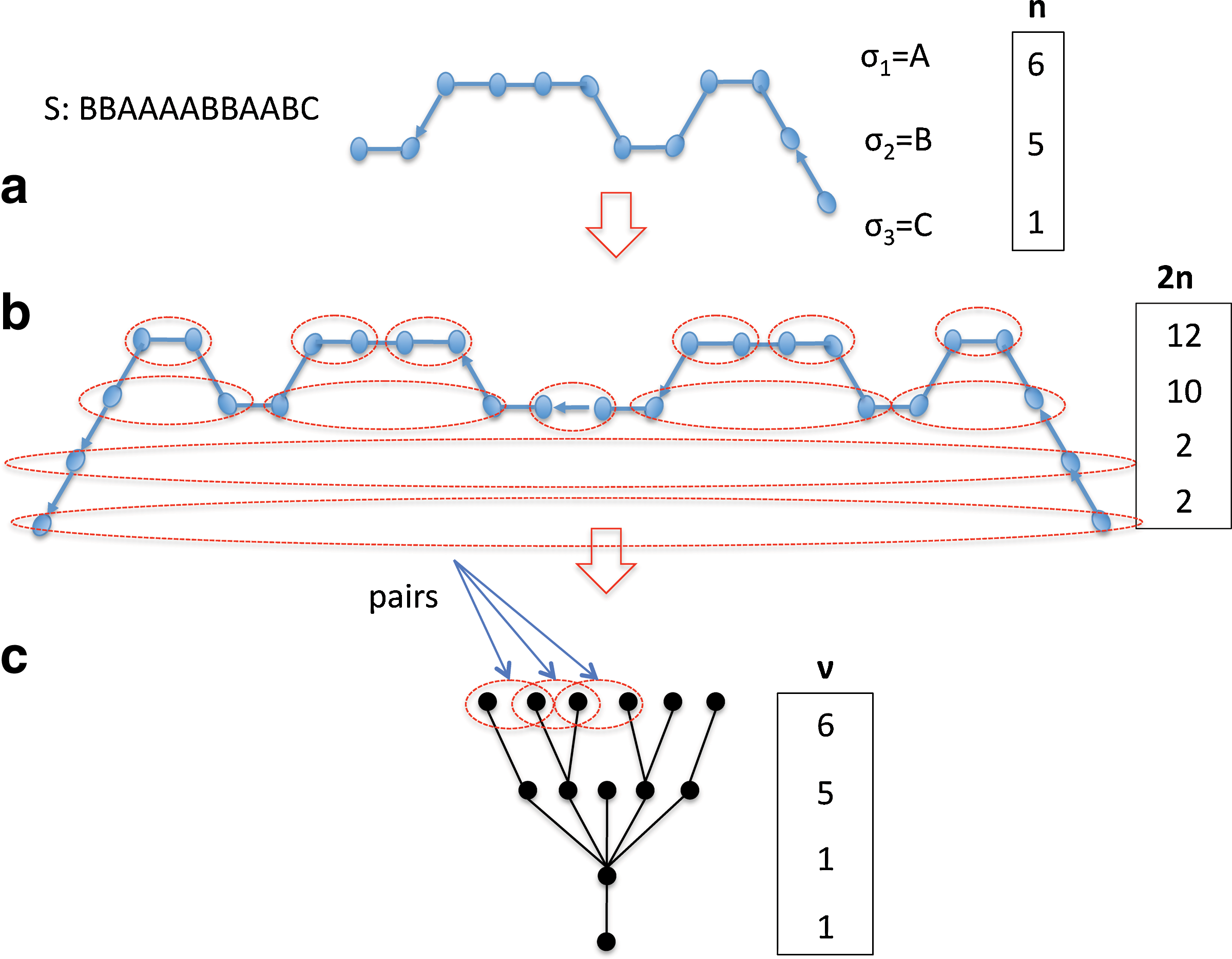
BFB-tree generated from an RB-BFB-schedule. (a) A graph for BBAAAABBAABC that supports [6, 5, 1]. (b) A single BFB operation begets an RB-BFB graph for [12, 10, 2, 2]. Dotted ellipses denote the nodes of a BFB-tree. (c) A BFB-tree for the BFB-string, with 3 levels. The single node at level 3 has 5 children, ordered as {−2,−1,0,1,2}. Pairs are illustrated at levels 1 and 2.

We use this idea to define rooted labeled trees. Each node is labeled so all nodes an identical distance from the root have the same label. For a node v with 2ℓ + 1 (odd) children, number the child nodes as \documentclass{aastex}\usepackage{amsbsy}\usepackage{amsfonts}\usepackage{amssymb}\usepackage{bm}\usepackage{mathrsfs}\usepackage{pifont}\usepackage{stmaryrd}\usepackage{textcomp}\usepackage{portland, xspace}\usepackage{amsmath, amsxtra}\pagestyle{empty}\DeclareMathSizes{10}{9}{7}{6}\begin{document} $$v_{- \ell} , \ldots v_0 , \dots , v_{\ell}$$ \end{document} . For a node with 2ℓ children the child nodes are labeled \documentclass{aastex}\usepackage{amsbsy}\usepackage{amsfonts}\usepackage{amssymb}\usepackage{bm}\usepackage{mathrsfs}\usepackage{pifont}\usepackage{stmaryrd}\usepackage{textcomp}\usepackage{portland, xspace}\usepackage{amsmath, amsxtra}\pagestyle{empty}\DeclareMathSizes{10}{9}{7}{6}\begin{document} $$v_{- \ell} , \ldots , v_{- 1} , v_1 , \ldots , v_{\ell}$$ \end{document} ; there is no v₀ node. T(v) denotes the subtree rooted at v. Define a labeled-traversal of T(r), as the string obtained by traversing the labels in an ordered, depth-first-search as given below: ▪

Algorithm 3
LabelTraverse(T(r))

Input: A labeled tree rooted at r

Output: The string given by a labeled traversal

1. Let σ = Label(r)

2. Let S₁ = ɛ

3. for (each child r_j ordered from least to max)

4. S₁ = S₁ · LabelTraverse(T (r_j))

5. return σS₁σ

A labeled tree is mirror-symmetric if for all nodes v, LabelTraverse(T(v)) = LabelTraverse(T(v))⁻¹. In other words, ‘rotation’ at v results in the same tree. The labeled traversal of a tree T visits each node exactly twice, outputting its label each time. Define a partial order on the nodes of T in which u < v if the last appearance of u precedes the first appearance of v in the labeled traversal. For any u < v, let T < (u, v) denote the subtree of T containing the LCA of u, v and all nodes w s.t. u < w < v. We call (u, v), with u < v, a label-pair if u and v have the same label σ, and no node in T < (u, v) has label σ. A labeled tree is pair-symmetric if for all label-pairs (u, v), T < (u, v) is mirror-symmetric. Finally, we say a labeled tree has long-ends if starting from the root, and following the least numbered node at each step, we can reach each layer k, \documentclass{aastex}\usepackage{amsbsy}\usepackage{amsfonts}\usepackage{amssymb}\usepackage{bm}\usepackage{mathrsfs}\usepackage{pifont}\usepackage{stmaryrd}\usepackage{textcomp}\usepackage{portland, xspace}\usepackage{amsmath, amsxtra}\pagestyle{empty}\DeclareMathSizes{10}{9}{7}{6}\begin{document} $$k - 1 , \ldots , 2 , 1$$ \end{document} .

Definition 1

A BFB-tree is a labeled tree with long-ends, mirror-symmetry, and pair-symmetry.

Theorem 8

Let T(r) be a BFB-tree rooted at r. Then LabeledTraversal (T(r)) is an RB-BFB-string.

Proof. Recall that a BFB-string is a string composed of overlapping palindromes such that the left edge of one palindrome is the center of the subsequent palindrome. Because T(r) is a BFB-tree, it is mirror-symmetric. Thus, the label traversal beginning from r will yield a string composed of nested palindromes. And, at any level of the tree, the label traversal will yield a set of concatenated palindromic return-blocks.

Because T(r) has long-ends, we know that the label traversal of each return-block does not contain any characters lexicographically higher than its initial ordered substring. For example, the return-block DCBBCCBBCD begins with BCD and hence cannot contain any A's. So, if there are two consecutive return-blocks such that the highest character in the return-block on the left is not higher than the highest character in the return-block on the right, there is a palindrome centered between the two return-blocks that extends to another palindrome center on the left. For example, if we have DCBBCCBBCDDCBAABCD, we have two return-blocks: DCBBCCBBCD and DCBAABCD. And, between them, there is the palindrome BCDDCB whose left edge is the center of the palindrome CBBC. So, we are able to find a set of appropriately overlapping palindromes.

On the other hand, if there are two consecutive return blocks such that the highest character in the return-block on the left is higher than the highest character in the return-block on the right, pair-symmetry guarantees that there is still a palindrome that extends left to another palindrome center. For example, the string CBAABCCBBCCBAABC is composed of three return-blocks: CBAABC, CBBC, and CBAABC. Pair-symmetry ensures that there is a palindrome that reaches to the center of the leftmost return-block, in this case ABCCBBCCBA.

Thus, the structure of T(r) guarantees that its label traversal is composed of overlapping palindromes and is thus a BFB-string. ▪

Theorem 9

The tree T _S derived from an RB-BFB-string S is a BFB-tree.

Proof. By Lemma 5, we have that each return-block is palindromic. This ensures that the label traversal of the tree rooted at any node is palindromic, and thus the T_S has mirror-symmetry. By Lemma 6, we have that each return-block is a BFB-string. By definition, a BFB-string begins with all characters that appear in the string in lexicographical order. Thus, from any node v in T_S, we can follow edges to the least-numbered child to reach the deepest node in T_S(v). Hence, T_S has long-ends. Finally, if there are whole return-blocks between two consecutive instances of the same character in S, then the concatenation of those return-blocks must be palindromic. Otherwise, no palindrome could include both instances of the character. Thus, T_S has pair-symmetry. ▪

The BFB-Tree Algorithm. Given a count-vector \documentclass{aastex}\usepackage{amsbsy}\usepackage{amsfonts}\usepackage{amssymb}\usepackage{bm}\usepackage{mathrsfs}\usepackage{pifont}\usepackage{stmaryrd}\usepackage{textcomp}\usepackage{portland, xspace}\usepackage{amsmath, amsxtra}\pagestyle{empty}\DeclareMathSizes{10}{9}{7}{6}\begin{document} $$\vec{n} = [n_1 , n_2 , \ldots , n_k] \ (\sum\nolimits_{i}n_i = n)$$ \end{document} , the BFB-Tree algorithm builds a BFB-tree on n + 1 nodes, with the count of nodes in each layer given by \documentclass{aastex}\usepackage{amsbsy}\usepackage{amsfonts}\usepackage{amssymb}\usepackage{bm}\usepackage{mathrsfs}\usepackage{pifont}\usepackage{stmaryrd}\usepackage{textcomp}\usepackage{portland, xspace}\usepackage{amsmath, amsxtra}\pagestyle{empty}\DeclareMathSizes{10}{9}{7}{6}\begin{document} $$\vec{\nu} = [n_1 , n_2 , \ldots , n_k , 1]$$ \end{document} . We start with the single node BFB-tree T at level k + 1, and extend it layer by layer. In each step j, 1 ≤ j ≤ k, we assign n_j children to the leaves of the current tree T , maintaining BFB-properties.

Denote the children of node v by the set \documentclass{aastex}\usepackage{amsbsy}\usepackage{amsfonts}\usepackage{amssymb}\usepackage{bm}\usepackage{mathrsfs}\usepackage{pifont}\usepackage{stmaryrd}\usepackage{textcomp}\usepackage{portland, xspace}\usepackage{amsmath, amsxtra}\pagestyle{empty}\DeclareMathSizes{10}{9}{7}{6}\begin{document} $$C_v = \{v_{- \ell} , \ldots , v_{\ell} \}$$ \end{document} . Mirror-symmetry ensures that for each 0 ≤ i ≤ ℓ , the subtrees T(v_−i) and T(v_i) are identical. Thus, it can be said the subtree T (v_−i) is dependent on the subtree T (v_i). We maintain this information by defining multiplicity, I(v), for each node as follows: I(r) = 1 for the root node r. For nodes v with children \documentclass{aastex}\usepackage{amsbsy}\usepackage{amsfonts}\usepackage{amssymb}\usepackage{bm}\usepackage{mathrsfs}\usepackage{pifont}\usepackage{stmaryrd}\usepackage{textcomp}\usepackage{portland, xspace}\usepackage{amsmath, amsxtra}\pagestyle{empty}\DeclareMathSizes{10}{9}{7}{6}\begin{document} $$v_{- \ell} , \ldots , v_{\ell}$$ \end{document} , set I(v_j) = 2I(v) for ℓ ≥ j > 0, I(v₀) = I(v), I(v_j) = 0 otherwise. That is, for child nodes v_j with a corresponding dependent child v_−j we assign a multiplicity of double the parent's multiplicity. For nodes with an odd number of children, there will be a child v₀ without a corresponding dependant child node. This node is assigned the same multiplicity as the parent node. Finally, for each dependent node pair, one is assigned a multiplicity of zero since, by mirror-symmetry, it is completely defined by its dependent whose multiplicity has doubled. Valid assignments at level j must then satisfy the diophantine equations Σ_vI_v = n_j+1, and Σ_vI(v)|C_v| = n_j.

Algorithm 3
BFB-Tree(T, j, I)

1. if j = 0, return CheckBFB(LabeledTraversal(T))

2. for each assignment C_v s.t. Σ_vI(v)|C_v| = n_j

3. Extend T according to the assignment

4. Adjust I

5. if (Construct_BFB_tree(T, j − 1, I)) return true

6. return false

Note that once a node is dependent (I(v) = 0), its descendants remain dependent. Further, the multiplicity of the node is a power of 2, and is doubled each time an independent node is a non-central child of its parent. As the multiplicities increase, the number of valid assignments decreases quickly, improving the running time in practice. Further analysis of the algorithm is presented in the appendix.

Rules for BFB. In addition to the two algorithms for solving the BFB count-vector problem presented above, it is also possible that some combinatorial rules completely define the set of count-vectors that admit a BFB schedule. We present seven conditions below that can guarantee that a BFB-schedule exists or does not exist for a subset of possible count-vectors.

Consider a count-vector \documentclass{aastex}\usepackage{amsbsy}\usepackage{amsfonts}\usepackage{amssymb}\usepackage{bm}\usepackage{mathrsfs}\usepackage{pifont}\usepackage{stmaryrd}\usepackage{textcomp}\usepackage{portland, xspace}\usepackage{amsmath, amsxtra}\pagestyle{empty}\DeclareMathSizes{10}{9}{7}{6}\begin{document} $$\vec{n} = [n_1 , n_2 , \ldots , n_k]$$ \end{document} . We use \documentclass{aastex}\usepackage{amsbsy}\usepackage{amsfonts}\usepackage{amssymb}\usepackage{bm}\usepackage{mathrsfs}\usepackage{pifont}\usepackage{stmaryrd}\usepackage{textcomp}\usepackage{portland, xspace}\usepackage{amsmath, amsxtra}\pagestyle{empty}\DeclareMathSizes{10}{9}{7}{6}\begin{document} $$BFB (\vec{n})$$ \end{document} to denote that \documentclass{aastex}\usepackage{amsbsy}\usepackage{amsfonts}\usepackage{amssymb}\usepackage{bm}\usepackage{mathrsfs}\usepackage{pifont}\usepackage{stmaryrd}\usepackage{textcomp}\usepackage{portland, xspace}\usepackage{amsmath, amsxtra}\pagestyle{empty}\DeclareMathSizes{10}{9}{7}{6}\begin{document} $$\vec{n}$$ \end{document} admits a BFB schedule.

Lemma 10

[Subsequence Rule] Let \documentclass{aastex}\usepackage{amsbsy}\usepackage{amsfonts}\usepackage{amssymb}\usepackage{bm}\usepackage{mathrsfs}\usepackage{pifont}\usepackage{stmaryrd}\usepackage{textcomp}\usepackage{portland, xspace}\usepackage{amsmath, amsxtra}\pagestyle{empty}\DeclareMathSizes{10}{9}{7}{6}\begin{document} $$\vec{n}^{\prime}$$ \end{document} be a subsequence of \documentclass{aastex}\usepackage{amsbsy}\usepackage{amsfonts}\usepackage{amssymb}\usepackage{bm}\usepackage{mathrsfs}\usepackage{pifont}\usepackage{stmaryrd}\usepackage{textcomp}\usepackage{portland, xspace}\usepackage{amsmath, amsxtra}\pagestyle{empty}\DeclareMathSizes{10}{9}{7}{6}\begin{document} $$\vec{n}. \ BFB (\vec{n}) \Rightarrow BFB (\vec{n}^{\prime})$$ \end{document} .

For example, if (6,4,6,8) admits a BFB schedule, then so must (6,4,6), (6,6,8), (6,4,8), (4,6,8), etc.

Proof. As discussed above, a BFB string is composed of palindromes that overlap so that the end of one palindrome is the center of the next palindrome. If all instances of a particular character are removed, the palindromes will still exist and have this property. So, the string will still be a BFB string. And, the character counts associated with the string will be a subsequence of the counts of the original string. ▪

Lemma 11

[Rule of One] If ∃ i < j ≤ k such that n_i = 1, n_j > 1, then \documentclass{aastex}\usepackage{amsbsy}\usepackage{amsfonts}\usepackage{amssymb}\usepackage{bm}\usepackage{mathrsfs}\usepackage{pifont}\usepackage{stmaryrd}\usepackage{textcomp}\usepackage{portland, xspace}\usepackage{amsmath, amsxtra}\pagestyle{empty}\DeclareMathSizes{10}{9}{7}{6}\begin{document} $$\lnot{BFB} (\vec{n})$$ \end{document} .

Proof. In order for the j^th character to achieve a count greater than one, it must be part of a prefix inversion/duplication. If the j^th character is in the prefix, then so is the i^th. But, the i^th character has a count of one, so it can never be part of a prefix inversion/duplication. ▪

Lemma 12

[Odd-Even Rule] If ∃i ≤ j ≤ k such that n_i is odd and n_j is even, then \documentclass{aastex}\usepackage{amsbsy}\usepackage{amsfonts}\usepackage{amssymb}\usepackage{bm}\usepackage{mathrsfs}\usepackage{pifont}\usepackage{stmaryrd}\usepackage{textcomp}\usepackage{portland, xspace}\usepackage{amsmath, amsxtra}\pagestyle{empty}\DeclareMathSizes{10}{9}{7}{6}\begin{document} $$\lnot{BFB} (\vec{n})$$ \end{document} .

Proof. We will consider the case where k = 2 and n₁ is odd and n₂ is even. So, we start with AB and need to get an odd count of As and an even count of B's.

We will show that, in a string yielded by any BFB schedule, the number of A's to the right of any B is even. First consider the trivial case where the B in question is the rightmost B. Then the number of A's to the right of that B is zero, which is even.

Now, suppose there is only one run A's to the right of the B in question, B₁. Then the string is \documentclass{aastex}\usepackage{amsbsy}\usepackage{amsfonts}\usepackage{amssymb}\usepackage{bm}\usepackage{mathrsfs}\usepackage{pifont}\usepackage{stmaryrd}\usepackage{textcomp}\usepackage{portland, xspace}\usepackage{amsmath, amsxtra}\pagestyle{empty}\DeclareMathSizes{10}{9}{7}{6}\begin{document} \begin{align} B_1 (B)_m (A)_nB_2 \end{align} \end{document}

where m > = 0 and (A)_n means a string of n A's.

In this case, B₁ can only have been generated after a copying of B₂. When B₂ was copied, it doubled the count of A's before B₂. So, n must be even.

Finally consider the case when there are arbitrarily many runs of A's after the given B, and all but the leftmost run contain an even number of A's \documentclass{aastex}\usepackage{amsbsy}\usepackage{amsfonts}\usepackage{amssymb}\usepackage{bm}\usepackage{mathrsfs}\usepackage{pifont}\usepackage{stmaryrd}\usepackage{textcomp}\usepackage{portland, xspace}\usepackage{amsmath, amsxtra}\pagestyle{empty}\DeclareMathSizes{10}{9}{7}{6}\begin{document} \begin{align} \ldots B_1 (B)_n (A)_k (B)_n (A)_{2i} (B)_{\ell} \ldots (A)_{2j}B_2 \end{align} \end{document}

In this case B₁ could only have been generated after a copying of a run of B's to the right of ( A )_k . This copying doubled the previous number of A's, so k is even. Since k is even and the counts of all other runs of A's are even, then the total count of A's to the right of B₁ is even. The result that the number of A's to the right of any B is even then follows by induction.

Similar reasoning can establish that the count of B's to the right of any A is odd. When a BFB schedule begins, A can be duplicated arbitrarily many times before B is duplicated for the first time, yielding \documentclass{aastex}\usepackage{amsbsy}\usepackage{amsfonts}\usepackage{amssymb}\usepackage{bm}\usepackage{mathrsfs}\usepackage{pifont}\usepackage{stmaryrd}\usepackage{textcomp}\usepackage{portland, xspace}\usepackage{amsmath, amsxtra}\pagestyle{empty}\DeclareMathSizes{10}{9}{7}{6}\begin{document} \begin{align} B (A)_m B \end{align} \end{document}

In this case, the count of B's to the right of any A is 1, which is odd. Now, consider the case where there are only two runs of B's after a given A. One of those runs must be the original B, so we have \documentclass{aastex}\usepackage{amsbsy}\usepackage{amsfonts}\usepackage{amssymb}\usepackage{bm}\usepackage{mathrsfs}\usepackage{pifont}\usepackage{stmaryrd}\usepackage{textcomp}\usepackage{portland, xspace}\usepackage{amsmath, amsxtra}\pagestyle{empty}\DeclareMathSizes{10}{9}{7}{6}\begin{document} \begin{align} \ldots A_1 (A)_k (B)_n (A)_m B \end{align} \end{document}

Using the reasoning above, n must be even because A₁ could only have been generated after a copying of an A from (A)_m, which would have doubled the B's leading to the run (B)_n.

In the case where there are arbitrarily many runs of B's after an A, and all of the runs have an even number of B's except the leftmost run and the rightmost run of length 1. Then, the count of B's to the right of every A is odd.

Now, return to the question of whether a BFB schedule can create a final string with an odd number of A's and and even number of B's. The final string ends in either A or B. If it ends in A, then the count of B's is odd because the count of B's to the right of the last A must be odd. But, we want the count of B's to be even, so the string cannot end in A. If the string ends in B, then the total count of A's must be even, but we want the count of A's to be odd. So, there is no string resulting from a BFB schedule where the count of A is odd and the count of B is even.

By using the Subsequence Rule, we can extend this result to conclude that no odd count can precede an even count in a count-vector achievable by BFB. ▪

Lemma 13

[Rule of Four] Suppose, all counts in \documentclass{aastex}\usepackage{amsbsy}\usepackage{amsfonts}\usepackage{amssymb}\usepackage{bm}\usepackage{mathrsfs}\usepackage{pifont}\usepackage{stmaryrd}\usepackage{textcomp}\usepackage{portland, xspace}\usepackage{amsmath, amsxtra}\pagestyle{empty}\DeclareMathSizes{10}{9}{7}{6}\begin{document} $$\vec{n}$$ \end{document} are even. Let i be the index of the first count that is not divisible by four, that is \documentclass{aastex}\usepackage{amsbsy}\usepackage{amsfonts}\usepackage{amssymb}\usepackage{bm}\usepackage{mathrsfs}\usepackage{pifont}\usepackage{stmaryrd}\usepackage{textcomp}\usepackage{portland, xspace}\usepackage{amsmath, amsxtra}\pagestyle{empty}\DeclareMathSizes{10}{9}{7}{6}\begin{document} $$4 \ n_i$$ \end{document} and ∀ j < i 4|j. Let f_ℓ be the number of times that divisibility by four changes in \documentclass{aastex}\usepackage{amsbsy}\usepackage{amsfonts}\usepackage{amssymb}\usepackage{bm}\usepackage{mathrsfs}\usepackage{pifont}\usepackage{stmaryrd}\usepackage{textcomp}\usepackage{portland, xspace}\usepackage{amsmath, amsxtra}\pagestyle{empty}\DeclareMathSizes{10}{9}{7}{6}\begin{document} $$n_i , \ldots , n_{\ell}$$ \end{document} . If \documentclass{aastex}\usepackage{amsbsy}\usepackage{amsfonts}\usepackage{amssymb}\usepackage{bm}\usepackage{mathrsfs}\usepackage{pifont}\usepackage{stmaryrd}\usepackage{textcomp}\usepackage{portland, xspace}\usepackage{amsmath, amsxtra}\pagestyle{empty}\DeclareMathSizes{10}{9}{7}{6}\begin{document} $$f_{\ell} > \frac {n_{\ell}} {2}$$ \end{document} then \documentclass{aastex}\usepackage{amsbsy}\usepackage{amsfonts}\usepackage{amssymb}\usepackage{bm}\usepackage{mathrsfs}\usepackage{pifont}\usepackage{stmaryrd}\usepackage{textcomp}\usepackage{portland, xspace}\usepackage{amsmath, amsxtra}\pagestyle{empty}\DeclareMathSizes{10}{9}{7}{6}\begin{document} $$\lnot BFB (\vec{n})$$ \end{document} .

Proof. Suppose that \documentclass{aastex}\usepackage{amsbsy}\usepackage{amsfonts}\usepackage{amssymb}\usepackage{bm}\usepackage{mathrsfs}\usepackage{pifont}\usepackage{stmaryrd}\usepackage{textcomp}\usepackage{portland, xspace}\usepackage{amsmath, amsxtra}\pagestyle{empty}\DeclareMathSizes{10}{9}{7}{6}\begin{document} $$f_{\ell} > \frac {n_{\ell}} {2}$$ \end{document} . Consider only counts that come before n_ℓ so that the character corresponding to n_ℓ is the base character. Then, the corresponding BFB-string will be composed of \documentclass{aastex}\usepackage{amsbsy}\usepackage{amsfonts}\usepackage{amssymb}\usepackage{bm}\usepackage{mathrsfs}\usepackage{pifont}\usepackage{stmaryrd}\usepackage{textcomp}\usepackage{portland, xspace}\usepackage{amsmath, amsxtra}\pagestyle{empty}\DeclareMathSizes{10}{9}{7}{6}\begin{document} $$\frac {n_{\ell}} {2}$$ \end{document} return-blocks. By Lemmas 5 and 6, each return-block is a palindrome and a BFB-string. By the Suffix Lemma, the right half of each return-block is also a BFB-string. The Odd-Even Rule tells us that no odd count precedes an even count in each half-return-block. So, no count not divisible by four precedes a count divisible by four within a return-block. Thus, after each return-block, the number of times that divisibility by four changes in the remaining counts can be decremented by at most one. ▪

Lemma 14

[Two Reduction] If n_i = 2 for some i. Then, \documentclass{aastex}\usepackage{amsbsy}\usepackage{amsfonts}\usepackage{amssymb}\usepackage{bm}\usepackage{mathrsfs}\usepackage{pifont}\usepackage{stmaryrd}\usepackage{textcomp}\usepackage{portland, xspace}\usepackage{amsmath, amsxtra}\pagestyle{empty}\DeclareMathSizes{10}{9}{7}{6}\begin{document} \begin{align} BFB (\vec {n}) \Leftrightarrow BFB ([\frac {1} {2} n_1 , \ldots , \frac {1} {2} n_{i - 1}]) \bigwedge BFB ([n_k - 1 , n_{k - 1} - 1, \ldots , n_i - 1]) \end{align} \end{document}

Proof. Consider a set of counts a, b, 2, d, e that starts with the string ABCDE. At some point, the C must be part of a prefix inversion/duplication so that it can achieve a count of 2. After that, no C can be part of any subsequent prefix inversion/duplication, as that would increase its count above 2. At that point, all A's and B's will be after a C, so no A or B can be part of a subsequent prefix inversion/duplication either. And, the duplication of the C would have also duplicated all existing A's and B's. So, a BFB schedule yielding \documentclass{aastex}\usepackage{amsbsy}\usepackage{amsfonts}\usepackage{amssymb}\usepackage{bm}\usepackage{mathrsfs}\usepackage{pifont}\usepackage{stmaryrd}\usepackage{textcomp}\usepackage{portland, xspace}\usepackage{amsmath, amsxtra}\pagestyle{empty}\DeclareMathSizes{10}{9}{7}{6}\begin{document} $$\frac {a} {2}$$ \end{document} , \documentclass{aastex}\usepackage{amsbsy}\usepackage{amsfonts}\usepackage{amssymb}\usepackage{bm}\usepackage{mathrsfs}\usepackage{pifont}\usepackage{stmaryrd}\usepackage{textcomp}\usepackage{portland, xspace}\usepackage{amsmath, amsxtra}\pagestyle{empty}\DeclareMathSizes{10}{9}{7}{6}\begin{document} $$\frac {b} {2}$$ \end{document} must be part of the overall BFB schedule yielding a, b, 2, d, e.

Now, if d > 1 or e > 1, then D and E must also be duplicated the first time C is duplicated. If they were not, then the string after the C duplication would be C[AB]CDE, and all D's and E's would be after a C and therefore ineligible to be part of any prefix inversion/duplication. So, the string must be EDC[AB]CDE, and subsequent prefix inversion/duplications will not extend past the final ED. The subsequent BFB schedule must achieve counts of e − 1 and d − 1 for E and D, respectively. ▪

Lemma 15

[Four Reduction] If ∃ i < j < k s.t. n_i = 4, n_k = 4, and n_j > 4. Then \documentclass{aastex}\usepackage{amsbsy}\usepackage{amsfonts}\usepackage{amssymb}\usepackage{bm}\usepackage{mathrsfs}\usepackage{pifont}\usepackage{stmaryrd}\usepackage{textcomp}\usepackage{portland, xspace}\usepackage{amsmath, amsxtra}\pagestyle{empty}\DeclareMathSizes{10}{9}{7}{6}\begin{document} $$BFB (\vec {n}) \Rightarrow BFB (\frac {n_1} {2} , \frac {n_2} {2} , \ldots , \frac {n_i} {2})$$ \end{document} .

Lemma 16

[Odd Reduction] Suppose all counts in \documentclass{aastex}\usepackage{amsbsy}\usepackage{amsfonts}\usepackage{amssymb}\usepackage{bm}\usepackage{mathrsfs}\usepackage{pifont}\usepackage{stmaryrd}\usepackage{textcomp}\usepackage{portland, xspace}\usepackage{amsmath, amsxtra}\pagestyle{empty}\DeclareMathSizes{10}{9}{7}{6}\begin{document} $$\vec{n}$$ \end{document} are odd. Then, \documentclass{aastex}\usepackage{amsbsy}\usepackage{amsfonts}\usepackage{amssymb}\usepackage{bm}\usepackage{mathrsfs}\usepackage{pifont}\usepackage{stmaryrd}\usepackage{textcomp}\usepackage{portland, xspace}\usepackage{amsmath, amsxtra}\pagestyle{empty}\DeclareMathSizes{10}{9}{7}{6}\begin{document} $$BFB (\vec{n}) \Rightarrow BFB (reverse (\vec{n} - \vec{1}))$$ \end{document} .

We also have a sufficient condition for BFB( \documentclass{aastex}\usepackage{amsbsy}\usepackage{amsfonts}\usepackage{amssymb}\usepackage{bm}\usepackage{mathrsfs}\usepackage{pifont}\usepackage{stmaryrd}\usepackage{textcomp}\usepackage{portland, xspace}\usepackage{amsmath, amsxtra}\pagestyle{empty}\DeclareMathSizes{10}{9}{7}{6}\begin{document} $$\vec{n}$$ \end{document} ).

Lemma 17

[Count Threshold Rule] BFB ( \documentclass{aastex}\usepackage{amsbsy}\usepackage{amsfonts}\usepackage{amssymb}\usepackage{bm}\usepackage{mathrsfs}\usepackage{pifont}\usepackage{stmaryrd}\usepackage{textcomp}\usepackage{portland, xspace}\usepackage{amsmath, amsxtra}\pagestyle{empty}\DeclareMathSizes{10}{9}{7}{6}\begin{document} $$\vec{n}$$ \end{document} ) if for all i n_i is even, and n_i > 2(i − 1).

Once the rules have been applied, we apply BFB-Pivot or BFB-Tree. Note that some of these rules are reductions, that is, they reduce an instance of the count-vector problem to simpler instances. These can be applied multiple times. More detail is available in the appendix.

4. Results

Performance on realistic data-sets. Using practical sized examples, we investigated the performance of the 3 approaches to checking BFB: rules, BFB-Pivot, and BFB-Tree. We applied the BFB rules to all \documentclass{aastex}\usepackage{amsbsy}\usepackage{amsfonts}\usepackage{amssymb}\usepackage{bm}\usepackage{mathrsfs}\usepackage{pifont}\usepackage{stmaryrd}\usepackage{textcomp}\usepackage{portland, xspace}\usepackage{amsmath, amsxtra}\pagestyle{empty}\DeclareMathSizes{10}{9}{7}{6}\begin{document} $$\sum\nolimits_{i = 1}^5 20^i = 3 , 368 , 420$$ \end{document} count-vectors with k ≤ 5 and each n_i ≤ 20. Remarkably, the rules were able to resolve 3,034,440, or 90%, of the count-vectors. As BFB-Pivot and BFB-Tree are both exponential time procedures, this check helped speed up the entire study.

Nearly all of the count-vectors that the rules could not resolve admitted a BFB schedule (Table 1), so BFB-Pivot and BFB-Tree could usually halt once an acceptable BFB string was found rather than exhausting all possible paths or trees.

Table 1.
Method and Result for the Count-Vectors Used to Analyze Algorithm Speed

Rules Tree/pivot Total

Admits BFB 170,576 333,840 504,416 (15.0%)

Not BFB 2,863,864 140 2,864,004 (85.0%)

Total 3,034,440 333,980 3,368,420

Fraction (90.1%) (9.9%)

We ran BFB-Pivot and BFB-Tree on each of the 333,980 count-vectors that could not be resolved by rules. The running times plotted against n for each algorithm is shown in Figure 4. As expected, both algorithms' worst-case running times grew exponentially with n. However, the worst case running times for BFB-Tree were orders of magnitude lower than for BFB-Pivot. For example, the longest running count-vector for BFB-Tree was [20,3,19,19,19] which took 10 seconds to complete. The longest running count-vector for BFB-Pivot was [20,18,20,20,6] which took 23,790 seconds to complete.

FIG. 4.
Pivot (left) and tree (right) algorithm running time. Each point refers to the size and running time of a specific example. The line represents median running time. Note that since the rules excluded nearly all count-vectors that did not admit a BFB schedule, almost all points are blue.

Consequences for experimental interpretation. Consider experimental data, such as array CGH or read mapping depth of coverage, that reveal the copy counts of segments of a chromosome arm, or in the terminology of this article, a count-vector. If this count-vector admits a BFB schedule, one might infer from this observation that BFB occurred.

On its face, this is a reasonable conclusion. Only 15% of the count-vectors with k ≤ 5 admit a BFB schedule. If we expand that analysis to the 64,000,000 count-vectors with k = 6 and n_i ≤ 20, only 7.3% admit a BFB schedule. So, it is plausible that observing a count-vector that admits a BFB schedule is much more likely if BFB did in fact occur. However, using our model of BFB, we show that this inference is usually incorrect.

Note first that experimentally derived count-vectors are often imprecise. Experiment typically provides a small range of values for each element in the count-vector rather than a single definite value. This is a result of the imprecision of the experimental method as well as potentially high levels of structural variation or aneuploidy in the genome being studied. Therefore, the observation made about the data may not be that a particular count-vector admits a BFB schedule but that there is a count-vector that admits a BFB schedule “nearby,” that is, within experimental precision of the observed count-vector.

Further, the uncertainty in a count tends to increase with the magnitude of the count. It is easier to distinguish between copy counts 1 versus 2 than between 32 versus 33. For simplicity, we assume that the relationship between uncertainty and magnitude is linear and use the Canberra distance (Deza and Deza, 2009) to compare count-vectors: \documentclass{aastex}\usepackage{amsbsy}\usepackage{amsfonts}\usepackage{amssymb}\usepackage{bm}\usepackage{mathrsfs}\usepackage{pifont}\usepackage{stmaryrd}\usepackage{textcomp}\usepackage{portland, xspace}\usepackage{amsmath, amsxtra}\pagestyle{empty}\DeclareMathSizes{10}{9}{7}{6}\begin{document} \begin{align} d (x , y) = \sum_{i} {\frac {\mid x_i - y_i \mid} {\mid x_i \mid + \mid y_i \mid}} \tag {2} \end{align} \end{document}

For each of the 64,000,000 count-vectors with 6 segments, we searched for the nearest count-vector that admits a BFB schedule and recorded the distance to that count-vector. For the 7.2% of count-vectors that admit a BFB schedule, the distance was, of course, zero. The distribution of distances is shown in Figure 5.

FIG. 5.
(Left) Distribution of distances to nearest count-vector admitting a BFB schedule. (Right) Percentage of count-vectors at least as close to a count-vector admitting a BFB schedule as the shown count-vector pair.

The results are striking. Consider the count-vector [14, 7, 18, 16, 9, 12], which does not admit a BFB-schedule. The nearest count-vector that does is [14, 7, 19, 17, 9, 13], at a distance of .097. Half of all count-vectors tested were at least this close to a count-vector admitting a BFB-schedule. So, if the precision of the experimental method employed is such that it can not reliably discern between a copy count of 12 and a copy count of 13 or a copy count of 18 and a copy count of 19, then half of the count-vectors we examined would appear to admit a BFB schedule. Similarly, if the method can not reliably discern a copy count of 9 and and 8 or 7 and 8, then 70% of count-vectors will appear to admit a BFB schedule. Fig. 5 has distances and and example vector pairs for additional percentiles.

Thus, even with small amounts experimental uncertainty, a majority of count-vectors admit a BFB schedule, so mechanisms other than BFB are likely to produce count-vectors that look like they were created by BFB. Therefore, finding a count-vector consistent with BFB should only slightly increase one's belief that BFB occurred.

On the other hand, observing a count-vector that is distant from any BFB admitting count-vector, provides strong evidence that BFB was not the cause of the amplification. The likelihood of observing a count-vector that is distant from a count-vector that admits a BFB schedule is low in any case, and is surely even lower if the chromosome arm underwent BFB.

5. Discussion

We present perhaps the first formalization of the BFB mechanism. Our main result is that BFB can result in a surprisingly broad range of amplification patterns along a chromosome arm. Indeed, for most contiguous patterns of amplification, it is possible to find a BFB schedule that yields either the given pattern or one that is very similar. As a result, one must be cautious when interpreting copy count data as evidence for BFB. The presence of amplification at all, or the presence of a terminal deletion from a chromosome arm can both suggest the occurrence of BFB, though they may not distinguish well between BFB and other amplification hypotheses. However, unless the counts are known precisely, a specific pattern of copy counts along the chromosome arm cannot offer compelling support for BFB.

This study suggests several avenues for future work. There are other types of evidence that can be deployed to argue that BFB has occurred. FISH can reveal, to some extent, the arrangement of segments along a chromosome arm. Next-generation sequencing can reveal the copy counts of breakpoints between rearranged chromosomal segments and may allow for a fuller characterization of a chromosome arm. Methods similar to those presented in this paper may prove useful for evaluating and interpreting these different types of evidence. Modeling may also be helpful for evaluating proposed refinements to models of BFB.

Finally, we have outlined two algorithms for determining whether a count-vector admits a BFB schedule, but neither is polynomial in reasonable measures of the input size. This problem, along with related problems, is interesting as computational problems per se. We hope in the future to have either faster solutions to these problems or proofs of hardness.

6. Appendix

A. Proofs

Theorem 3

Algorithm CheckBFB checks if x is a BFB-string in O(n) time.

Proof. (Maximal Palindromes) A string is a BFB-string if and only if it can be formed by an inverted prefix duplication from another BFB-string or it is the original string, x⁰. An inverted prefix duplication forms an even palindrome at the beginning of a string. CheckBFB finds such a palindrome and then, in effect, recurses on the string that ends at that palindrome's center. The Suffix Lemma guarantees that that string must be a BFB-string if x is a BFB-string. If a string does not begin with a palindrome, and it is not x⁰, then it is not a BFB-string.

We would like to describe an algorithm that finds the radius of the largest palindrome centered at each interstice in a string in linear time. We will, in fact, describe two. The first lends itself to clear exposition and establishes that the problem can be solved in linear time. The second lends itself to easier implementation and is the method we used for results in this paper.

Our first algorithm has three steps and is similar to the algorithm described by Gusfield (1997).
1. Build a generalized suffix tree from the string and the reverse of the string, that is, a suffix tree that contains both suffixes and prefixes of the string. As usual, each leaf corresponding to a suffix beginning at position i is labeled i. Each leaf corresponding to a prefix ending at i is labeled −i. It is well known this can be done in linear time.

2. For each position in the string, i, find the lowest common ancestor of i and −i. Using Tarjan's algorithm, this can be done with linear preprocessing time and constant query time (Harel and Tarjan, 1984).

3. Find the distance from the root to the LCA. This is the size of the largest common prefix ending and i and suffix starting at i and hence radius of the largest palindrome.

While this is indeed a linear time algorithm to find maximal palindromes, Tarjan's algorithm is not considered to be particularly implementable. So, we implemented another linear time algorithm that is similar to Manacher's algorithm (Manacher, 1975). This algorithm proceeds through each interstice in the string, from left to right. As each interstice, is visited, pairs of characters at the boundary of the current known palindrome are tested to see if that palindrome can be expanded. If it cannot, then the palindrome radius is appended to the R array. Then, for each interstice to the right lying in the radius of this palindrome, the corresponding maximal palindrome size for the interstice lying to the left is checked. If the maximal palindrome to the left lies completely within the radius of the current palindrome, then we know that the radius of the maximal palindrome to the right is equal to the radius of the maximal palindrome on the left. If the maximal palindrome on the left is a proper prefix of the current palindrome or it extends beyond the radius of the current palindrome, then the corresponding palindrome on the right has a radius that extends at least to the current palindrome's radius.

Algorithm 5
MaximalPalindromes

Input: String s

Output: Array of integers R, the maximal palindrome radii.

1. i = 0

2. ℓ = 0

3. n = len(s)

4. while i + ℓ < n − 1

5. do if s[i−ℓ] = s[i+ℓ+1]

6. then ℓ++

7. continue

8. R.append(ℓ)

9. c = 0

10. foundSuffix = False

11. for 0 ≤ i′ < ℓ − 1

12. do if ℓ − i′ − 1 ≤ R(i − i′ − 1)

13. then ℓ = ℓ − i′ − 1

14. foundSuffix = True

15. break

16. R.append(min(ℓ − i′ − 1,R(i − i′ − 1))

17. c ++

18. if not foundSuffix

19. then ℓ = 0

20. i + = c + 1

21. return R

Note that if the first if clause is true, then ℓ is incremented by one. If the inner loop iterates all ℓ times, then ℓ is set to zero and i is increased by ℓ + 1. If the inner loop finds a palindromic suffix and breaks, then ℓ is set to ℓ − i′ − 1 and i is set to i + i′ + 2. In all three cases, i + ℓ is incremented by one in each iteration of the outer loop. Therefore the outer loop only iterates n times. The inner loop appends a value to R in iteration and thus is called at most n − 1 times. Thus, MaximalPalindromes is in O(n).

Finally, note that both algorithms presented above give us the radius of largest palindrome measured from the center of the palindrome. The algorithm CheckBFB uses the length of largest palindrome measured from its leftmost character to its center, so we need to convert the R array we get from MaximalPalindromes to the P array used by CheckBFB. This can easily be done in linear time:

Algorithm 6
RtoP

Input: R array (palindrome radii)

Output: P array (palindrome lengths from left)

1. ( * Instantiate P array to all zeroes * )

2. P = [0](R.length() + 1)

3. for 0 < i ≤ R.length()

4. do P[i − R[i] + 1] = max(P[i − R[i] + 1], R[i])

5. pal_counter = 0

6. for 0 < i < P.length()

7. do pal_counter = max(P[i], pal_counter − 1, 0)

8. P[i] = max(P[i], pal_counter)

9. return P

RtoP reads through the R array once. Each time it finds a nonzero palindrome radius, it updates the appropriate element in the P array. Then, it reads through the P array once and updates each value so it is the maximum of its current value or the appropriately decremented value for a palindrome that contains the element. ▪

B. Applying BFB rules

Some of the rules are “reductions” rather than simple tests if a count-vector admits a BFB schedule. This means that they show that a count-vector admits a BFB schedule if (and sometimes only if ) some set of simpler count-vectors all admit a BFB schedule. We therefore apply these rules in a recursive fashion outlined below:

Algorithm 7
ApplyRules*

Input: \documentclass{aastex}\usepackage{amsbsy}\usepackage{amsfonts}\usepackage{amssymb}\usepackage{bm}\usepackage{mathrsfs}\usepackage{pifont}\usepackage{stmaryrd}\usepackage{textcomp}\usepackage{portland, xspace}\usepackage{amsmath, amsxtra}\pagestyle{empty}\DeclareMathSizes{10}{9}{7}{6}\begin{document} $$\vec{n}$$ \end{document} a count-vector

Output: true if \documentclass{aastex}\usepackage{amsbsy}\usepackage{amsfonts}\usepackage{amssymb}\usepackage{bm}\usepackage{mathrsfs}\usepackage{pifont}\usepackage{stmaryrd}\usepackage{textcomp}\usepackage{portland, xspace}\usepackage{amsmath, amsxtra}\pagestyle{empty}\DeclareMathSizes{10}{9}{7}{6}\begin{document} $$\vec{n}$$ \end{document} admits a BFB schedule, false if \documentclass{aastex}\usepackage{amsbsy}\usepackage{amsfonts}\usepackage{amssymb}\usepackage{bm}\usepackage{mathrsfs}\usepackage{pifont}\usepackage{stmaryrd}\usepackage{textcomp}\usepackage{portland, xspace}\usepackage{amsmath, amsxtra}\pagestyle{empty}\DeclareMathSizes{10}{9}{7}{6}\begin{document} $$\vec{n}$$ \end{document} does not admit a BFB schedule, or R a set of count-vectors such that \documentclass{aastex}\usepackage{amsbsy}\usepackage{amsfonts}\usepackage{amssymb}\usepackage{bm}\usepackage{mathrsfs}\usepackage{pifont}\usepackage{stmaryrd}\usepackage{textcomp}\usepackage{portland, xspace}\usepackage{amsmath, amsxtra}\pagestyle{empty}\DeclareMathSizes{10}{9}{7}{6}\begin{document} $$\vec{n}$$ \end{document} admits a BFB schedule iff every count-vector in R does

1. if \documentclass{aastex}\usepackage{amsbsy}\usepackage{amsfonts}\usepackage{amssymb}\usepackage{bm}\usepackage{mathrsfs}\usepackage{pifont}\usepackage{stmaryrd}\usepackage{textcomp}\usepackage{portland, xspace}\usepackage{amsmath, amsxtra}\pagestyle{empty}\DeclareMathSizes{10}{9}{7}{6}\begin{document} $$\vec{n}$$ \end{document} passes CountThresholdRule return true

2. if \documentclass{aastex}\usepackage{amsbsy}\usepackage{amsfonts}\usepackage{amssymb}\usepackage{bm}\usepackage{mathrsfs}\usepackage{pifont}\usepackage{stmaryrd}\usepackage{textcomp}\usepackage{portland, xspace}\usepackage{amsmath, amsxtra}\pagestyle{empty}\DeclareMathSizes{10}{9}{7}{6}\begin{document} $$\vec{n}$$ \end{document} fails RuleOfOne, OddEvenRule, or DivByFourRule return false

3. \documentclass{aastex}\usepackage{amsbsy}\usepackage{amsfonts}\usepackage{amssymb}\usepackage{bm}\usepackage{mathrsfs}\usepackage{pifont}\usepackage{stmaryrd}\usepackage{textcomp}\usepackage{portland, xspace}\usepackage{amsmath, amsxtra}\pagestyle{empty}\DeclareMathSizes{10}{9}{7}{6}\begin{document} $$\vec{o} = OddReduction (\vec{n})$$ \end{document}

4. if \documentclass{aastex}\usepackage{amsbsy}\usepackage{amsfonts}\usepackage{amssymb}\usepackage{bm}\usepackage{mathrsfs}\usepackage{pifont}\usepackage{stmaryrd}\usepackage{textcomp}\usepackage{portland, xspace}\usepackage{amsmath, amsxtra}\pagestyle{empty}\DeclareMathSizes{10}{9}{7}{6}\begin{document} $$\vec{o}.length () = \vec{n}.length ()$$ \end{document}

5. ( * If the whole count-vector is odd * )

6. then return ApplyRules( \documentclass{aastex}\usepackage{amsbsy}\usepackage{amsfonts}\usepackage{amssymb}\usepackage{bm}\usepackage{mathrsfs}\usepackage{pifont}\usepackage{stmaryrd}\usepackage{textcomp}\usepackage{portland, xspace}\usepackage{amsmath, amsxtra}\pagestyle{empty}\DeclareMathSizes{10}{9}{7}{6}\begin{document} $$\vec{o}$$ \end{document} )

7. else if not ApplyRules( \documentclass{aastex}\usepackage{amsbsy}\usepackage{amsfonts}\usepackage{amssymb}\usepackage{bm}\usepackage{mathrsfs}\usepackage{pifont}\usepackage{stmaryrd}\usepackage{textcomp}\usepackage{portland, xspace}\usepackage{amsmath, amsxtra}\pagestyle{empty}\DeclareMathSizes{10}{9}{7}{6}\begin{document} $$\vec{o}$$ \end{document} )

8. then return false

9. \documentclass{aastex}\usepackage{amsbsy}\usepackage{amsfonts}\usepackage{amssymb}\usepackage{bm}\usepackage{mathrsfs}\usepackage{pifont}\usepackage{stmaryrd}\usepackage{textcomp}\usepackage{portland, xspace}\usepackage{amsmath, amsxtra}\pagestyle{empty}\DeclareMathSizes{10}{9}{7}{6}\begin{document} $$\vec{f} = FourReduction (\vec{n})$$ \end{document}

10. if not ApplyRules( \documentclass{aastex}\usepackage{amsbsy}\usepackage{amsfonts}\usepackage{amssymb}\usepackage{bm}\usepackage{mathrsfs}\usepackage{pifont}\usepackage{stmaryrd}\usepackage{textcomp}\usepackage{portland, xspace}\usepackage{amsmath, amsxtra}\pagestyle{empty}\DeclareMathSizes{10}{9}{7}{6}\begin{document} $$\vec{f}$$ \end{document} ) return false

11. \documentclass{aastex}\usepackage{amsbsy}\usepackage{amsfonts}\usepackage{amssymb}\usepackage{bm}\usepackage{mathrsfs}\usepackage{pifont}\usepackage{stmaryrd}\usepackage{textcomp}\usepackage{portland, xspace}\usepackage{amsmath, amsxtra}\pagestyle{empty}\DeclareMathSizes{10}{9}{7}{6}\begin{document} $$\vec{p} , \vec{s} = TwoReduction (\vec{n})$$ \end{document}

12. if \documentclass{aastex}\usepackage{amsbsy}\usepackage{amsfonts}\usepackage{amssymb}\usepackage{bm}\usepackage{mathrsfs}\usepackage{pifont}\usepackage{stmaryrd}\usepackage{textcomp}\usepackage{portland, xspace}\usepackage{amsmath, amsxtra}\pagestyle{empty}\DeclareMathSizes{10}{9}{7}{6}\begin{document} $$\vec{p}$$ \end{document} or \documentclass{aastex}\usepackage{amsbsy}\usepackage{amsfonts}\usepackage{amssymb}\usepackage{bm}\usepackage{mathrsfs}\usepackage{pifont}\usepackage{stmaryrd}\usepackage{textcomp}\usepackage{portland, xspace}\usepackage{amsmath, amsxtra}\pagestyle{empty}\DeclareMathSizes{10}{9}{7}{6}\begin{document} $$\vec{s}$$ \end{document} not empty

13. then if not ApplyRules( \documentclass{aastex}\usepackage{amsbsy}\usepackage{amsfonts}\usepackage{amssymb}\usepackage{bm}\usepackage{mathrsfs}\usepackage{pifont}\usepackage{stmaryrd}\usepackage{textcomp}\usepackage{portland, xspace}\usepackage{amsmath, amsxtra}\pagestyle{empty}\DeclareMathSizes{10}{9}{7}{6}\begin{document} $$\vec{p}$$ \end{document} ) or not ApplyRules( \documentclass{aastex}\usepackage{amsbsy}\usepackage{amsfonts}\usepackage{amssymb}\usepackage{bm}\usepackage{mathrsfs}\usepackage{pifont}\usepackage{stmaryrd}\usepackage{textcomp}\usepackage{portland, xspace}\usepackage{amsmath, amsxtra}\pagestyle{empty}\DeclareMathSizes{10}{9}{7}{6}\begin{document} $$\vec{s}$$ \end{document} ) return false

14. if ApplyRules( \documentclass{aastex}\usepackage{amsbsy}\usepackage{amsfonts}\usepackage{amssymb}\usepackage{bm}\usepackage{mathrsfs}\usepackage{pifont}\usepackage{stmaryrd}\usepackage{textcomp}\usepackage{portland, xspace}\usepackage{amsmath, amsxtra}\pagestyle{empty}\DeclareMathSizes{10}{9}{7}{6}\begin{document} $$\vec{p}$$ \end{document} ) and ApplyRules( \documentclass{aastex}\usepackage{amsbsy}\usepackage{amsfonts}\usepackage{amssymb}\usepackage{bm}\usepackage{mathrsfs}\usepackage{pifont}\usepackage{stmaryrd}\usepackage{textcomp}\usepackage{portland, xspace}\usepackage{amsmath, amsxtra}\pagestyle{empty}\DeclareMathSizes{10}{9}{7}{6}\begin{document} $$\vec{s}$$ \end{document} ) return true

15. else return ApplyRules( \documentclass{aastex}\usepackage{amsbsy}\usepackage{amsfonts}\usepackage{amssymb}\usepackage{bm}\usepackage{mathrsfs}\usepackage{pifont}\usepackage{stmaryrd}\usepackage{textcomp}\usepackage{portland, xspace}\usepackage{amsmath, amsxtra}\pagestyle{empty}\DeclareMathSizes{10}{9}{7}{6}\begin{document} $$\vec{p}$$ \end{document} ) ∪ ApplyRules( \documentclass{aastex}\usepackage{amsbsy}\usepackage{amsfonts}\usepackage{amssymb}\usepackage{bm}\usepackage{mathrsfs}\usepackage{pifont}\usepackage{stmaryrd}\usepackage{textcomp}\usepackage{portland, xspace}\usepackage{amsmath, amsxtra}\pagestyle{empty}\DeclareMathSizes{10}{9}{7}{6}\begin{document} $$\vec{s}$$ \end{document} )

16. return \documentclass{aastex}\usepackage{amsbsy}\usepackage{amsfonts}\usepackage{amssymb}\usepackage{bm}\usepackage{mathrsfs}\usepackage{pifont}\usepackage{stmaryrd}\usepackage{textcomp}\usepackage{portland, xspace}\usepackage{amsmath, amsxtra}\pagestyle{empty}\DeclareMathSizes{10}{9}{7}{6}\begin{document} $$\vec{n}$$ \end{document}

C. Analysis of BFB_tree

Let I(v) denote the multiplicity of a node v that is independent, and 0 otherwise. At step j of the algorithm, we must assign the n_j nodes at the current level to the independent nodes at level j − 1. Let n_jv be the nodes assigned to node v. Then, all assignments must satisfy \documentclass{aastex}\usepackage{amsbsy}\usepackage{amsfonts}\usepackage{amssymb}\usepackage{bm}\usepackage{mathrsfs}\usepackage{pifont}\usepackage{stmaryrd}\usepackage{textcomp}\usepackage{portland, xspace}\usepackage{amsmath, amsxtra}\pagestyle{empty}\DeclareMathSizes{10}{9}{7}{6}\begin{document} $$\sum\nolimits_v I (v) n_{jv} = n_j$$ \end{document} . We start with n_k = 1, and continue to the first level where the number of nodes is more than one. Upto this point, there is a unique assignment. For all subsequent levels j, the number of independent nodes at level j is at most \documentclass{aastex}\usepackage{amsbsy}\usepackage{amsfonts}\usepackage{amssymb}\usepackage{bm}\usepackage{mathrsfs}\usepackage{pifont}\usepackage{stmaryrd}\usepackage{textcomp}\usepackage{portland, xspace}\usepackage{amsmath, amsxtra}\pagestyle{empty}\DeclareMathSizes{10}{9}{7}{6}\begin{document} $$\lceil \frac {n_j} {2} \rceil$$ \end{document} , and except for the center node, each has a multiplicity of at least 2. The total number of assignments at the level is bounded by \documentclass{aastex}\usepackage{amsbsy}\usepackage{amsfonts}\usepackage{amssymb}\usepackage{bm}\usepackage{mathrsfs}\usepackage{pifont}\usepackage{stmaryrd}\usepackage{textcomp}\usepackage{portland, xspace}\usepackage{amsmath, amsxtra}\pagestyle{empty}\DeclareMathSizes{10}{9}{7}{6}\begin{document} \begin{align} {\lceil \frac {n_j} {2} \rceil + \lfloor \frac {n_{j - 1}} {2} \rfloor - 1 \choose \lfloor \frac {n_{j - 1}} {2} \rfloor} \le 2^{\frac {1} {2} (n_{j - 1} + n_{j})} \end{align} \end{document}

And the total number of trees considered is bounded by \documentclass{aastex}\usepackage{amsbsy}\usepackage{amsfonts}\usepackage{amssymb}\usepackage{bm}\usepackage{mathrsfs}\usepackage{pifont}\usepackage{stmaryrd}\usepackage{textcomp}\usepackage{portland, xspace}\usepackage{amsmath, amsxtra}\pagestyle{empty}\DeclareMathSizes{10}{9}{7}{6}\begin{document} \begin{align} \prod_j 2^{\frac {1} {2} (n_{j - 1} + n_{j})} \le 2^{\Sigma_j n_j} = 2^n \end{align} \end{document}

By definition, these assignments will satisfy mirror-symmetry, and the long-end property is easily checked as well. However, checking all pair-symmetry constraints at level j requires a single traversal of the tree.

However, the actual performance should be superior. The algorithm also requires maintaining the count-vector I. Note that I(r) = 1 for the root node r. For other nodes v with children \documentclass{aastex}\usepackage{amsbsy}\usepackage{amsfonts}\usepackage{amssymb}\usepackage{bm}\usepackage{mathrsfs}\usepackage{pifont}\usepackage{stmaryrd}\usepackage{textcomp}\usepackage{portland, xspace}\usepackage{amsmath, amsxtra}\pagestyle{empty}\DeclareMathSizes{10}{9}{7}{6}\begin{document} $$v_{- \ell} , \ldots , v_{\ell}$$ \end{document} \documentclass{aastex}\usepackage{amsbsy}\usepackage{amsfonts}\usepackage{amssymb}\usepackage{bm}\usepackage{mathrsfs}\usepackage{pifont}\usepackage{stmaryrd}\usepackage{textcomp}\usepackage{portland, xspace}\usepackage{amsmath, amsxtra}\pagestyle{empty}\DeclareMathSizes{10}{9}{7}{6}\begin{document} \begin{align} I (v_j) = \begin{cases}2I (v) \quad - \ell \le j < 0 \\ \\ I (v) \qquad j = 0 \\ \\ 0 \qquad \quad \hbox{otherwise}\end{cases} \end{align} \end{document}

Note that once a node is dependent (I(v) = 0), its descendants remain dependent. Further, the multiplicity of the node is a power of 2, and is doubled each time an independent node is a non-central child of its parent. As the multiplicities increase, the number of assignments decreases quickly, so that in practice, there will be very few valid assignments after the first few levels.

Specifically, consider an input data-set with k + 1 levels, a single node at level k + 1, and a maximum of m nodes at each of the k levels.

let I_t be the multiplicity of the left-most node at level t from a random assignment. The long-ends property ensures that I_t ≠ 0, Then, \documentclass{aastex}\usepackage{amsbsy}\usepackage{amsfonts}\usepackage{amssymb}\usepackage{bm}\usepackage{mathrsfs}\usepackage{pifont}\usepackage{stmaryrd}\usepackage{textcomp}\usepackage{portland, xspace}\usepackage{amsmath, amsxtra}\pagestyle{empty}\DeclareMathSizes{10}{9}{7}{6}\begin{document} \begin{align} I_t = \begin{cases}I_{t + 1} \quad \hbox{( v is the only child of its parent)} \\ \\ 2I_{t + 1} \ \ \hbox{( otherwise)}\end{cases} \end{align} \end{document}

It is not hard to show that I_t almost doubles with each round, and reaches the maximum value m after log₂(m) rounds. Once I_t = n, for some t there is only one assignment possible. Prior to that, the maximum number of assignments at each level is O(2^m). Therefore, the number of labeled trees with long-ends and mirror symmetry is bounded by \documentclass{aastex}\usepackage{amsbsy}\usepackage{amsfonts}\usepackage{amssymb}\usepackage{bm}\usepackage{mathrsfs}\usepackage{pifont}\usepackage{stmaryrd}\usepackage{textcomp}\usepackage{portland, xspace}\usepackage{amsmath, amsxtra}\pagestyle{empty}\DeclareMathSizes{10}{9}{7}{6}\begin{document} $$O (2^{m \log_2m})$$ \end{document} .

	Rules	Tree/pivot	Total
Admits BFB	170,576	333,840	504,416	(15.0%)
Not BFB	2,863,864	140	2,864,004	(85.0%)
Total	3,034,440	333,980	3,368,420
Fraction	(90.1%)	(9.9%)

Footnotes

Acknowledgments

This research was supported in part by grants from the NIH (5RO1-HG004962) and the NSF (CCF-1115206).

Disclosure Statement

No competing financial interests exist.

References

Artandi

S.E.

, DePinho

R.A.

2010. Telomeres and telomerase in cancer. Carcinogenesis, 31:9–18.

Bignell

G.R.

, Santarius

, Pole

J.C.

et al. 2007. Architectures of somatic genomic rearrangement in human cancer amplicons at sequence-level resolution. Genome Res., 17:1296–1303.

Deza

M.M.

, Deza

2009. Encyclopedia of Distances. Springer: New York.

Gusfield

1997. Algorithms on Strings, Trees and Sequences: Computer Science and Computational Biology. Cambridge University Press: New York.

Harel

, Tarjan

R.E.

1984. Fast algorithms for finding nearest common ancestors. SIAM J. Comput., 13:338–355.

Kitada

, Yamasaki

2008. The complicated copy number alterations in chromosome 7 of a lung cancer cell line is explained by a model based on repeated breakage-fusion-bridge cycles. Cancer Genet. Cytogenet., 185:11–19.

Manacher

1975. A new linear time on-line algorithm for finding the smallest initial palindrome of a string. J. Assoc. Comput. Mach., 22:346–351.

McClintock

1938. The production of homozygous deficient tissues with mutant characteristics by means of the aberrant mitotic behavior of ring-shaped chromosomes. Genetics, 23:315–376.

McClintock

1941. The stability of broken ends of chromosomes in Zea mays. Genetics, 26:234–282.

10.

Santarius

, Shipley

, Brewer

et al. 2010. A census of amplified and overexpressed human cancer genes. Nat. Rev. Cancer, 10:59–64.

11.

Shimizu

, Shingaki

, Kaneko-Sasaguri

et al. 2005. When, where and how the bridge breaks: anaphase bridge breakage plays a crucial role in gene amplification and HSR generation. Exp. Cell Res., 302:233–243.