SPAdes: A New Genome Assembly Algorithm and Its Applications to Single-Cell Sequencing

Abstract

The lion's share of bacteria in various environments cannot be cloned in the laboratory and thus cannot be sequenced using existing technologies. A major goal of single-cell genomics is to complement gene-centric metagenomic data with whole-genome assemblies of uncultivated organisms. Assembly of single-cell data is challenging because of highly non-uniform read coverage as well as elevated levels of sequencing errors and chimeric reads. We describe SPAdes, a new assembler for both single-cell and standard (multicell) assembly, and demonstrate that it improves on the recently released E+V−SC assembler (specialized for single-cell data) and on popular assemblers Velvet and SoapDeNovo (for multicell data). SPAdes generates single-cell assemblies, providing information about genomes of uncultivatable bacteria that vastly exceeds what may be obtained via traditional metagenomics studies. SPAdes is available online (http://bioinf.spbau.ru/spades). It is distributed as open source software.

1. Introduction

Most bacteria in environments ranging from the human body to the ocean cannot be cloned in the laboratory and thus cannot be sequenced using existing Next Generation Sequencing (NGS) technologies. This represents the key bottleneck for various projects ranging from the Human Microbiome Project (HMP) (Gill et al., 2006) to antibiotics discovery (Li and Vederas, 2009). For example, the key question in the HMP is how bacteria interact with each other. These interactions are often conducted by various peptides that are produced either for communication with other bacteria or for killing them. However, peptidomics studies of the human microbiome are now limited since mass spectrometry (the key technology for such studies) requires knowledge of fairly complete proteomes. On the other hand, while studies of new peptide antibiotics would greatly benefit from DNA sequencing of genes coding for Non-Ribosomal Peptide Syntetases (NRPS) (Sieber and Marahiel, 2005), existing metagenomics approaches are unable to sequence these exceptionally long genes (over 60,000 nucleotides).

HMP and discovery of new antibiotics are just two examples of many projects that would be revolutionized by Single-Cell Sequencing (SCS). Recent improvements in both experimental (Ishoey et al., 2008; Navin et al., 2011; Islam et al., 2011) and computational (Chitsaz et al., 2011) aspects of SCS have opened the possibility of sequencing bacterial genomes from single cells. In particular, Chitsaz et al. (2011) demonstrated that SCS can capture a large number of genes, sufficient for inferring the organism's metabolism. In many applications (including proteomics and antibiotics discovery), having a great majority of genes captured is almost as useful as having complete genomes.

Currently, Multiple Displacement Amplification (MDA) is the dominant technology for single-cell amplification (Dean et al., 2001). However, MDA introduces extreme amplification bias (orders-of-magnitude difference in coverage between different regions) and gives rise to chimeric reads and read-pairs that complicate the ensuing assembly.1 Acknowledging the fact that existing assemblers were not designed to handle these complications, Rodrigue et al. (2009) remarked that the challenges facing SCS are increasingly computational rather than experimental. Recent articles (Marcy et al., 2007; Woyke et al., 2010; Youssef et al., 2011; Blainey et al., 2011; Grindberg et al., 2011) illustrate the challenges of fragment assembly in SCS.

Chitsaz et al. (2011) introduced the E+V-SC assembler, combining a modified EULER-SR with a modified Velvet, and achieved a significant improvement in fragment assembly for SCS data. However, we (G.T. and P.A.P.), as coauthors of Chitsaz et al. (2011), realized that one needs to change algorithmic design (rather than just modify existing tools) to fully utilize the potential of SCS.

We present the SPAdes assembler, introducing a number of new algorithmic solutions and improving on state-of-the-art assemblers for both SCS and standard (multicell) bacterial datasets. Fragment assembly is often abstracted as the problem of reconstructing a string from the set of its k-mers. This abstraction naturally leads to the de Bruijn approach to assembly, the basis of many fragment assembly algorithms. However, a more advanced abstraction of NGS data considers the problem of reconstructing a string from a set of pairs of k-mers (called k-bimers below) at a distance ≈ d in a string. Unfortunately, while there is a simple algorithm for the former abstraction, analysis of the latter abstraction has mainly amounted to post-processing heuristics on de Bruijn graphs. While many heuristics for analysis of read-pairs (called bireads2 below) have been proposed (Pevzner et al., 2001; Pevzner and Tang, 2001; Zerbino and Birney, 2008; Butler et al., 2008; Simpson et al., 2009; Chaisson et al., 2009; Li et al., 2010), proper utilization of bireads remains, arguably, the most poorly explored stage of assembly. Medvedev et al. (2011a) recently introduced Paired de Bruijn graphs (PDBGs), a new approach better suited for the latter abstraction and having important advantages over standard de Bruijn graphs. However, PDBGs were introduced as a theoretical rather than practical idea, aimed mainly at the unrealistic case of a fixed distance between reads.

When Idury and Waterman (1995) introduced de Bruijn graphs for fragment assembly, many viewed this approach as impractical due to high error rates in Sanger reads.3 Pevzner et al. (2001) removed this bottleneck by introducing an error correction procedure that made the vast majority of reads error-free. Similarly, PDBGs may appear impractical due to variation in biread (and thus k-bimer) distances characteristic of NGS. SPAdes addresses this bottleneck by introducing k-bimer adjustment, which reveals exact distances for the vast majority of the adjusted k-bimers, and by introducing paired assembly graphs inspired by PDBGs. In particular, SPAdes is able to utilize read-pairs; E+V-SC used the reads but ignored the pairing in read-pairs to avoid misassembles caused by an elevated level of chimeric read-pairs.

We assume that the reader is familiar with the concept of A-Bruijn graphs introduced in Pevzner et al. (2004). De Bruijn graphs, PDBGs, and several other graphs in this paper are special cases of A-Bruijn graphs. SPAdes is a universal A-Bruijn assembler in the sense that it uses k-mers only for building the initial de Bruijn graph and “forgets” about them afterwards; on subsequent stages it only performs graph-theoretical operations on graphs that need not be labeled by k-mers. The operations are based on graph topology, coverage, and sequence lengths, but not the sequences themselves. At the last stage, the consensus DNA sequence is restored. We designed a universal assembler to implement several variations of A-Bruijn graphs (e.g., paired and multisized de Bruijn graphs) in the same framework, and to apply it to other applications where these graphs have proven to be useful (Bandeira et al., 2007, 2008; Pham and Pevzner, 2010).

In Section 2, we give an overview of the stages of SPAdes. In Section 3, we define de Bruijn graphs, multisized de Bruijn graphs, and PDBGs. Sections 4 –6 cover different stages of SPAdes. In Section 7, we benchmark SPAdes and other assemblers on single-cell and cultured E. coli datasets. In Section 8, we give additional details about assembly graph construction and data structures. In Section 9, we give a detailed example of constructing a paired assembly graph. In Section 10, we further discuss the concept of a universal assembler.

2. Assembly in SPAdes: An Outline

Below we outline the four stages of SPAdes, which deal with issues that are particularly troublesome in SCS: sequencing errors; non-uniform coverage; insert size variation; and chimeric reads and bireads:

(1) Stage 1 (assembly graph construction) is addressed by every NGS assembler and is often referred to as de Bruijn graph simplification (e.g., bulge/bubble removal in EULER/Velvet). We propose a new approach to assembly graph construction that uses the multisized de Bruijn graph, implements new bulge/tip removal algorithms, detects and removes chimeric reads, aggregates biread information into distance histograms, and allows one to backtrack the performed graph operations.

(2) Stage 2 (k-bimer adjustment) derives accurate distance estimates between k-mers in the genome (edges in the assembly graph) using joint analysis of distance histograms and paths in the assembly graph.

(3) Stage 3 constructs the paired assembly graph, inspired by the PDBG approach.

(4) Stage 4 (contig construction) was well studied in the context of Sanger sequencing (Ewing et al., 1998). Since NGS projects typically feature high coverage, NGS assemblers generate rather accurate contigs (although the accuracy deteriorates for SCS). SPAdes constructs DNA sequences of contigs and the mapping of reads to contigs by backtracking graph simplifications (see Section 8.6).

Previous studies demonstrated that coupling various assemblers with error correction tools improves their performance (Pevzner et al., 2001; Kelley et al., 2010; Ilie et al., 2010; Gnerre et al., 2011).4 However, most error correction tools (e.g., Quake [Kelley et al., 2010]) perform poorly on single-cell data since they implicitly assume nearly uniform read coverage. Chitsaz et al. (2011) coupled Velvet-SC with the error-correction in EULER (Chaisson and Pevzner, 2008), resulting in the tool E+V-SC. In this article, SPAdes uses a modification of Hammer (Medvedev et al., 2011b) (aimed at SCS) for error correction and quality trimming prior to assembly.5

Our paired assembly graph approach differs from existing approaches to assembly and dictates new algorithmic solutions for various stages of SPAdes. Thus, we will describe several variations of de Bruijn graphs, leading to construction of the paired assembly graph (covering stages 2 and 3), before describing Stage 1. Stage 4 will be presented in Section 8.6.

3. De Bruijn Graphs: Standard, Multisized, and Paired

3.1. Terminology

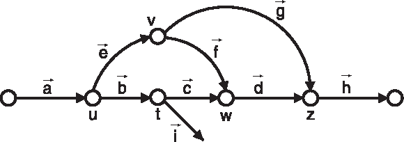
Since various assembly articles use widely different terminology, below we specify a terminology that is well suited for PDBGs. All graphs considered below are directed graphs. A vertex w precedes (follows) vertex v in a graph G if there exists an edge from w to v (from v to w) in G. indegree(v) (outdegree(v)) is the the number of vertices preceding (following) v. A vertex v in a graph G is called a hub if indegree(v) ≠ 1 or outdegree(v) ≠ 1. A directed path in G is called a hub-path (abbreviated h-path) if its starting and ending vertices are hubs and its intermediate vertices are not hubs. Obviously, each edge in the graph belongs to a unique h-path. An edge is called a hub-edge (abbreviated h-edge) if it starts at a hub. There is a correspondence between h-paths and h-edges: the first edge on each h-path is an h-edge, and the h-edge is unique to that h-path.6 Given an h-edge α, we define the h-path starting at α as path(α) and denote the number of edges in this h-path (h-path length) as |path(α)|. If a is the i-th edge in an h-path (1 ≤ i ≤ |path(α)|) starting from an h-edge α, we define h-edge(a) = α and offset(a) = i (Fig. 1).

FIG. 1.

Notation for decomposing a de Bruijn graph into non-branching paths (h-paths). A de Bruijn graph on reads ACCGT C AGAAT and ACCGT G AGAAT with edge size k = 4, vertex size k − 1 = 3. Hubs are shown as solid vertices, while vertices with indegree 1, outdegree 1 are hollow. An h-path CGT → GTG → TGA → GAG → AGA (shown in red with h-edge denoted α) defines an h-read CGTGAGA. The whole path is denoted path(α), and consists of |path(α)| = 4 edges. The edges on this path have offsets 1, 2, 3, 4, as indicated. Each edge can be addressed by its path's h-edge and its offset.

3.2. Standard de Bruijn graphs

An n-mer is a string of length n. Given an n-mer \documentclass{aastex}\usepackage{amsbsy}\usepackage{amsfonts}\usepackage{amssymb}\usepackage{bm}\usepackage{mathrsfs}\usepackage{pifont}\usepackage{stmaryrd}\usepackage{textcomp}\usepackage{portland, xspace}\usepackage{amsmath, amsxtra}\pagestyle{empty}\DeclareMathSizes{10}{9}{7}{6}\begin{document} $$a = (a_1, \ldots, a_n)$$ \end{document} , we define prefix \documentclass{aastex}\usepackage{amsbsy}\usepackage{amsfonts}\usepackage{amssymb}\usepackage{bm}\usepackage{mathrsfs}\usepackage{pifont}\usepackage{stmaryrd}\usepackage{textcomp}\usepackage{portland, xspace}\usepackage{amsmath, amsxtra}\pagestyle{empty}\DeclareMathSizes{10}{9}{7}{6}\begin{document} $$(a) = (a_1, \ldots, a_{n - 1})$$ \end{document} and suffix \documentclass{aastex}\usepackage{amsbsy}\usepackage{amsfonts}\usepackage{amssymb}\usepackage{bm}\usepackage{mathrsfs}\usepackage{pifont}\usepackage{stmaryrd}\usepackage{textcomp}\usepackage{portland, xspace}\usepackage{amsmath, amsxtra}\pagestyle{empty}\DeclareMathSizes{10}{9}{7}{6}\begin{document} $$(a) = (a_2, \ldots, a_n)$$ \end{document} .

For the rest of the paper, we fix a positive integer k. For a set Reads of strings (thought of as the DNA sequencing reads over the alphabet {A, C, G, T}), let N be the number of k-mers that occur in strings in Reads as substrings. We define the de Bruijn graph DB(Reads, k) as follows (Fig. 2):

D1. Define an initial graph G₀ on 2N vertices. For each k-mer a that occurs in strings in Reads as a substring, introduce two new vertices u, v and form an edge u → v. Label the new edge by a, u by prefix(a), and v by suffix(a). Note that we label edges by k-mers and vertices by (k − 1)-mers.

D2. Glue vertices of G₀ together if they have the same label.

FIG. 2.

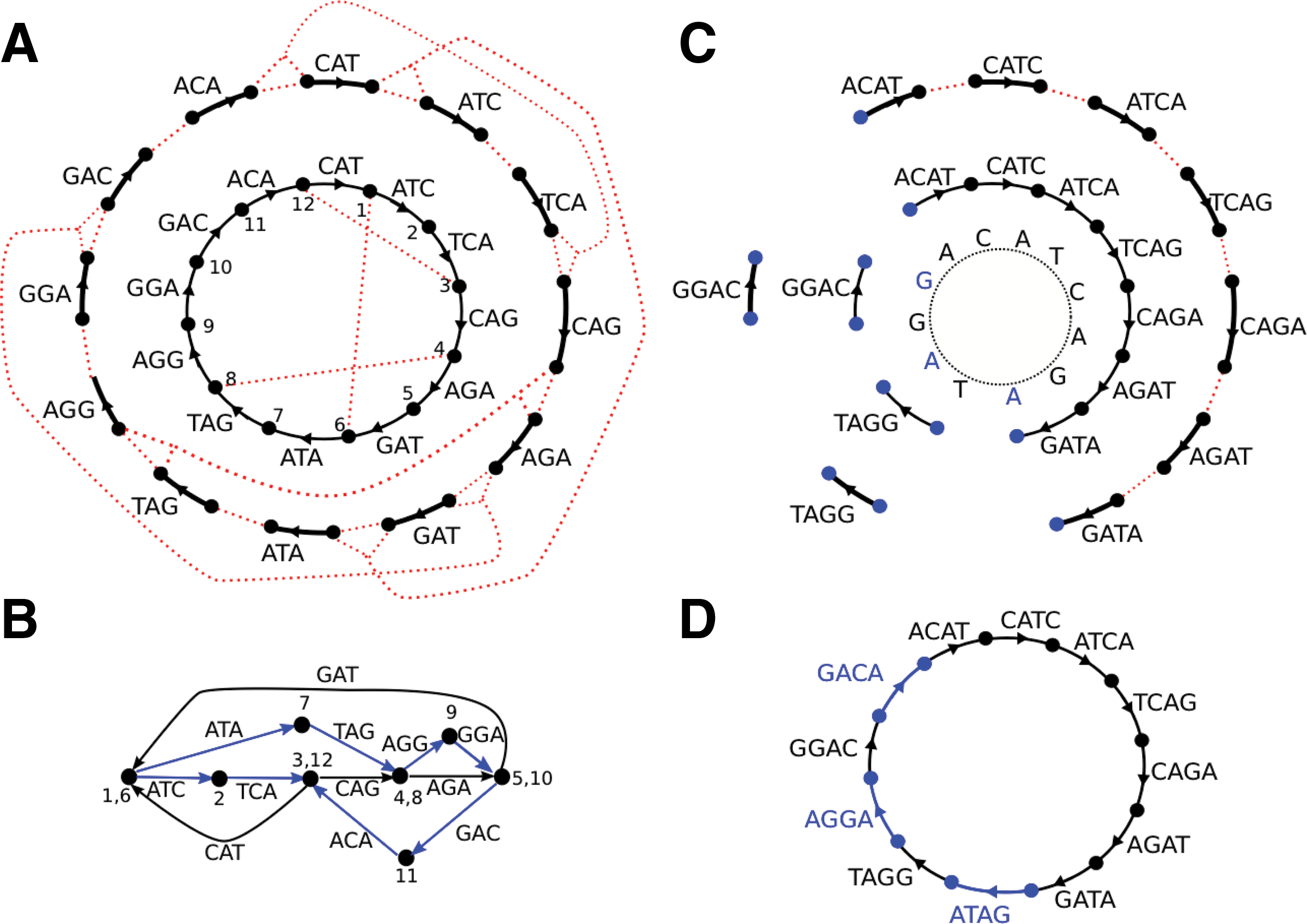
Standard and multisized de Bruijn graph. A circular Genome CATCAGATAGGA is covered by a set Reads consisting of nine 4-mers, {ACAT, CATC, ATCA, TCAG, CAGA, AGAT, GATA, TAGG, GGAC}. Three out of 12 possible 4-mers from Genome are missing from Reads (namely {ATAG,AGGA,GACA}), but all 3-mers from Genome are present in Reads. (A) The outside circle shows a separate black edge for each 3-mer from Reads. Dotted red lines indicate vertices that will be glued. The inner circle shows the result of applying some of the glues. (B) The graph DB(Reads, 3) resulting from all the glues is tangled. The three h-paths of length 2 in this graph (shown in blue) correspond to h-reads ATAG, AGGA, and GACA. Thus Reads_3,4 contains all 4-mers from Genome. (C) The outside circle shows a separate edge for each of the nine 4-mer reads. The next inner circle shows the graph DB(Reads, 4), and the innermost circle represents the Genome. The graph DB(Reads, 4) is fragmented into 3 connected components. (D) The multisized de Bruijn graph DB(Reads, 3, 4).

In the de Bruijn graph DB(Reads, k), an h-path passing through n vertices \documentclass{aastex}\usepackage{amsbsy}\usepackage{amsfonts}\usepackage{amssymb}\usepackage{bm}\usepackage{mathrsfs}\usepackage{pifont}\usepackage{stmaryrd}\usepackage{textcomp}\usepackage{portland, xspace}\usepackage{amsmath, amsxtra}\pagestyle{empty}\DeclareMathSizes{10}{9}{7}{6}\begin{document} $$(a_1, \ldots, a_{k - 1}) \rightarrow (a_2, \ldots, a_k) \rightarrow \ldots \rightarrow (a_n, \ldots, a_{n + k - 2})$$ \end{document} defines an (n + k − 2)-mer \documentclass{aastex}\usepackage{amsbsy}\usepackage{amsfonts}\usepackage{amssymb}\usepackage{bm}\usepackage{mathrsfs}\usepackage{pifont}\usepackage{stmaryrd}\usepackage{textcomp}\usepackage{portland, xspace}\usepackage{amsmath, amsxtra}\pagestyle{empty}\DeclareMathSizes{10}{9}{7}{6}\begin{document} $$(a_1, \ldots, a_{n + k - 2})$$ \end{document} called a hub-read (abbreviated h-read) (Fig. 1). Substituting every h-path in DB(Reads, k) by a single edge labeled by its h-read results in a condensed de Bruijn graph.

We define Reads_k as the set of all h-reads in DB(Reads, k). Obviously, DB(Reads, k) = DB(Reads_k, k).

We define the coverage of an edge in the de Bruijn graph DB(Reads, k) as the number of reads that contain the corresponding k-mer. The coverage of a path is defined as the average coverage of its edges.

3.3. Multisized de Bruijn graphs

The choice of k affects the construction of the de Bruijn graph. Smaller values of k collapse more repeats together, making the graph more tangled. Larger values of k may fail to detect overlaps between reads, particularly in low coverage regions, making the graph more fragmented. Since low coverage regions are typical for SCS data, the choice of k greatly affects the quality of single-cell assembly. Ideally, one should use smaller values of k in low-coverage regions (to reduce fragmentation) and larger values of k in high-coverage regions (to reduce repeat collapsing). The multisized de Bruijn graph (compare with Peng et al. [2010] and Gnerre et al. [2011]) allows us to vary k in this manner.

Given a positive integer δ < k, we define Reads_k-δ,k as the union of δ + 1 sets: \documentclass{aastex}\usepackage{amsbsy}\usepackage{amsfonts}\usepackage{amssymb}\usepackage{bm}\usepackage{mathrsfs}\usepackage{pifont}\usepackage{stmaryrd}\usepackage{textcomp}\usepackage{portland, xspace}\usepackage{amsmath, amsxtra}\pagestyle{empty}\DeclareMathSizes{10}{9}{7}{6}\begin{document} $$\textsc{Reads}_k \cup \textsc{Reads}_{k - 1} \cup\ldots \cup \textsc{Reads}_{k - \delta}$$ \end{document} . The multisized de Bruijn graph, DB(Reads, k−δ, k) is defined as DB(Reads_k-δ,k, k). Figure 2 shows the standard de Bruijn graphs DB(Reads, 3) (tangled) and DB(Reads, 4) (fragmented) as well as the multisized de Bruijn graph DB(Reads, 3, 4), which is neither tangled nor fragmented.

3.4. Practical paired de Bruijn graphs: k-bimer adjustment

In this presentation, we focus on a library with bireads having insert sizes in the range d_insert ± Δ. The genomic distance between two positions in a circular genome (and k-mers starting at these positions) is the difference of their coordinates modulo the genome length. For example, the genomic distance between a pair of reads of length ℓ oriented in the same direction with insert size d_insert is d_insert − ℓ. In the ensuing discussion, we will work with genomic distances between k-mers rather than insert sizes.

Medvedev et al. (2011a) introduced paired de Bruijn graphs (PDBG), a new approach to assembling bireads; similar approaches were recently proposed in Donmez and Brudno (2011) and Chikhi and Lavenier (2011). While PDBGs have advantages over standard de Bruijn graphs when the exact insert size is fixed, Medvedev et al. (2011a) acknowledged that PDBG-based assemblies deteriorate in practice for bireads with variable insert sizes and raised the problem of making PDBGs practical for insert size variations characteristic of current sequencing technologies.

Since it is still impractical to experimentally generate bireads with exact (or nearly exact) distances, we describe a computational approach that addresses the same goal. A k-bimer is a triple (a|b, d) consisting of k-mers a and b together with an integer d (estimated distance between particular instances of a and b in a genome). SPAdes first extracts k-bimers from bireads, resulting in k-bimers with inexact distance estimates (inherited from biread distance estimates). The k-bimer adjustment approach transforms this set of k-bimers (with rather inaccurate distance estimates) into a set of adjusted k-bimers with exact or nearly exact distance estimates. Similarly to error correction, which replaces original reads with virtual error-corrected reads (Pevzner et al., 2001), k-bimer adjustment substitutes original k-bimers by adjusted k-bimers. The adjusted k-bimer can be formed by two k-mers that were not parts of a single biread in the input data. We show that k-bimer adjustment improves accuracy of distance estimates and the resulting assembly.

4. Stage 2: Utilization of Read-Pairs in Spades

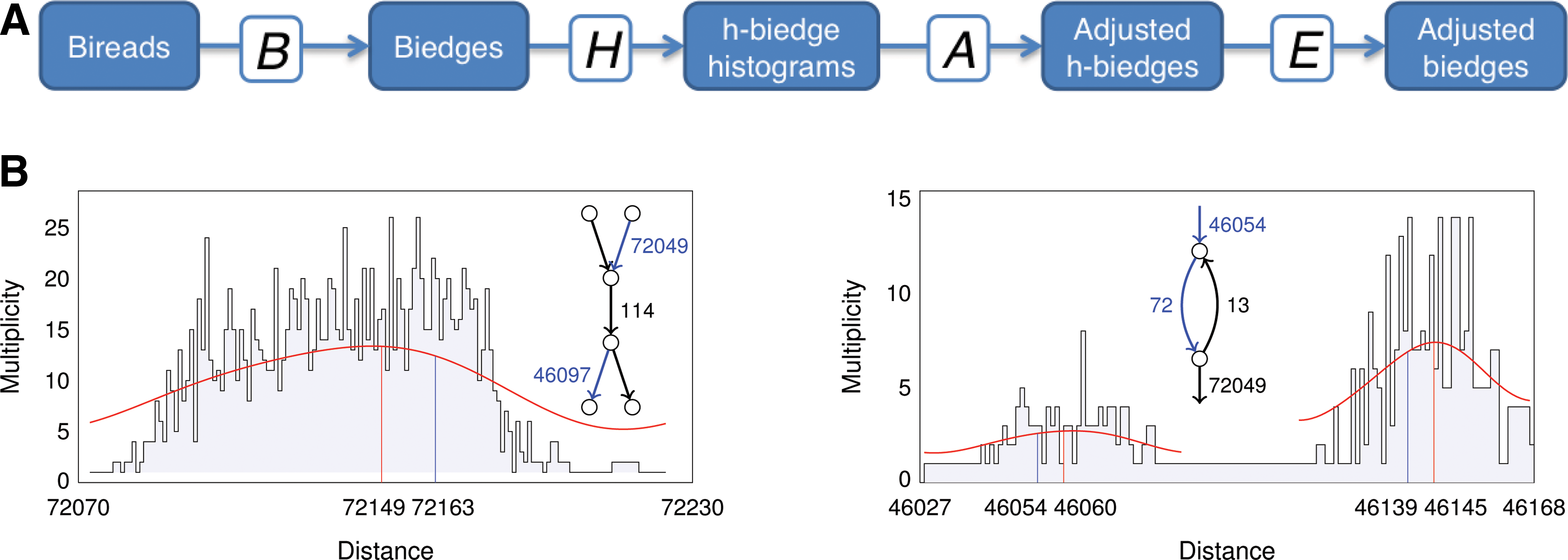
Let C be an Eulerian cycle7 in a multigraph G. The distance between edges a and b in cycle C is defined as the number of edges between Start(a) and Start(b) in the cycle C (Start(e) and End(e) refer to starting and ending vertices of an edge e). We define the distance between a pair of h-paths as the distance between their h-edges. When cycle C (in a de Bruijn graph) corresponds to a genome, the distance between edges corresponds to the genomic distance.

Below we assume that reads within bireads are separated by genomic distance ≈ d₀ (d₀ is fixed throughout the article). The genomic distance between a pair of h-paths (i.e., strings corresponding to these h-paths) can be estimated when they are linked by bireads (that is, the first read maps to the first h-path and the second read maps to the second h-path). The estimated genomic distances between the two reads in a biread are aggregated over all bireads connecting a given pair of h-paths, through a series of transformations (Fig. 3A). The B-transformation breaks bireads into k-bimers; the H-transformation shifts the genomic distance estimate of a k-bimer connecting two h-paths to a distance estimate for the pair of h-edges representing those two h-paths, and collects this into a histogram; the A-transformation analyzes the histogram of (imprecise) distance estimates between two h-paths to determine more precise distance estimates; and the E-transformation transforms the genomic distance estimate for a given pair of h-paths into a set of k-bimers. Applying these transformations to the initial set of bireads Bireads transforms it into a set of adjusted k-bimers E(A(H(B(Bireads)))). We give further details on these transformations as follows:

FIG. 3.

Stage 2 of SPAdes. (A) Bireads are decomposed into pairs of k-mers with estimated genomic distances (B-transformation). These are tabulated into histograms of estimated genomic distances between pairs of h-edges (H-transformation), and peaks in the histograms and paths in the graph are used to reveal the actual genomic distances between h-edges (A-transformation). This may be converted back to genomic distances between k-mers on pairs of h-paths (E-transformation, used for presentation purposes but not needed in the implementation). (B) The h-biedge histogram (α|β,*) corresponding to the exact h-biedge (α|β, 72163) in the assembly graph. path(α) is an h-path (condensed edge representing 72049 edges) in the upper right, and path(β) is an h-path (representing 46097 edges) at the lower left. The histogram collects all distance estimates between α and β derived from bireads. The h-biedge histogram was smoothed using the Fast Fourier Transform (red curve). The peak in the smoothed histogram (marked red) well approximates the actual distance (marked blue). (C) The h-biedge histogram (α|β,*) estimates the distance between h-edges α and β (|path(α)| = 46054, |path(β)| = 72). Because of the directed cycle formed by the two h-paths of lengths 72 and 13, there may be multiple walks through the graph between α and β. The h-biedge histogram has been divided into clusters with centers at 46060 and 46145. Thus SPAdes transforms the entire histogram into two h-biedges: (α|β, 46054) and (α|β, 46139).

4.1. B-transformation

Consider a pair of reads r₁ and r₂ at approximate genomic distance d₀ (inferred from the nominal insert length) and their mapping (described in Sec. 8.6) to paths p₁ and p₂ in the assembly graph. If p₁ and p₂ are subpaths of single h-paths in the assembly graph, we sample pairs of k-mers from these subpaths. If a k-mer a₁ (resp., a₂) is sampled from the read r₁ (resp., r₂), we form a k-bimer (a₁|a₂, d₀ − i₁ + i₂), where i₁ and i₂ are the starting positions of a₁ and a₂ in reads r₁ and r₂. If read r₁ (resp., r₂) is mapped to a path overlapping with n₁ (resp., n₂) h-paths in the assembly graph, we sample pairs of k-mers a₁ and a₂ from all n₁ × n₂ pairs of h-paths and form k-bimers (a₁|a₂, d₀ − i₁ + i₂) where i₁ and i₂ are the starting positions of a₁ and a₂ in reads r₁ and r₂.

Each k-bimer formed by applying the B-transformation to bireads defines a pair of edges in the de Bruijn graph, which we refer to as a biedge. Each biedge formed by edges residing on h-paths path(α) and path(β) implies a distance estimate D between h-edges α and β. This yields an h-biedge (α|β, D), constructed as follows:

4.2. H-transformation

Given a biedge (a|b, d), we define an h-biedge H(a|b, d) = (h-edge(a)|h-edge(b), D), where D = d + offset(a) - offset(b) represents the corresponding distance estimate between particular instances of k-mers h-edge(a) and h-edge(b) in the genome.

4.3. A-transformation

An h-biedge histogram (α|β,*) is a multiset of h-biedges with fixed h-edges α and β and variable distance estimates. Such histograms are generated by applying H-transformations to various biedges (a|b, d) with \documentclass{aastex}\usepackage{amsbsy}\usepackage{amsfonts}\usepackage{amssymb}\usepackage{bm}\usepackage{mathrsfs}\usepackage{pifont}\usepackage{stmaryrd}\usepackage{textcomp}\usepackage{portland, xspace}\usepackage{amsmath, amsxtra}\pagestyle{empty}\DeclareMathSizes{10}{9}{7}{6}\begin{document} $$a \in \textsc{path} (\alpha)$$ \end{document} and \documentclass{aastex}\usepackage{amsbsy}\usepackage{amsfonts}\usepackage{amssymb}\usepackage{bm}\usepackage{mathrsfs}\usepackage{pifont}\usepackage{stmaryrd}\usepackage{textcomp}\usepackage{portland, xspace}\usepackage{amsmath, amsxtra}\pagestyle{empty}\DeclareMathSizes{10}{9}{7}{6}\begin{document} $$b \in \textsc{path} (\beta)$$ \end{document} . SPAdes analyzes h-biedge histograms and also paths in the graph to derive accurate distance estimates between h-edges. Given an h-biedge histogram (α|β,*), we define the adjustment operation A(α|β,*), which transforms the histogram into a single adjusted h-biedge (α|β, D) or a small number of adjusted h- biedges (Fig. 3B,C). More details are below.

4.4. E-transformation

Given an h-biedge (α|β, D), we define E(α|β, D) as the set of all biedges (a|b, d) such that \documentclass{aastex}\usepackage{amsbsy}\usepackage{amsfonts}\usepackage{amssymb}\usepackage{bm}\usepackage{mathrsfs}\usepackage{pifont}\usepackage{stmaryrd}\usepackage{textcomp}\usepackage{portland, xspace}\usepackage{amsmath, amsxtra}\pagestyle{empty}\DeclareMathSizes{10}{9}{7}{6}\begin{document} $$a \in \textsc{path} (\alpha)$$ \end{document} , \documentclass{aastex}\usepackage{amsbsy}\usepackage{amsfonts}\usepackage{amssymb}\usepackage{bm}\usepackage{mathrsfs}\usepackage{pifont}\usepackage{stmaryrd}\usepackage{textcomp}\usepackage{portland, xspace}\usepackage{amsmath, amsxtra}\pagestyle{empty}\DeclareMathSizes{10}{9}{7}{6}\begin{document} $$b \in \textsc{path} (\beta)$$ \end{document} and d + offset(a) - offset(b) = D.

Given a set Bireads with exact distance d₀ between reads within bireads, one can transform it into a set H(B(Bireads)) of h-biedges with exact distances and further transform the resulting set into a set E(H(B(Bireads))) of k-bimers (the A-transformation is skipped since distances are exact). One can construct the PDBG of h-biedges in H(B(Bireads)) by simply constructing the PDBG of E(H(B(Bireads))) (Medvedev et al., 2011a).

When the distance estimate d₀ between reads within bireads (and between k-mers) is exact, the transformation of bireads (and k-bimers) into h-biedges yields an equivalent representation that has no advantages. However, h-biedges have an important advantage in the case of inexact distance estimates. In this case, h-edges provide a way to adjust k-bimers and thus reveal k-mers with an exact (or nearly exact) distance estimate, making the construction of PDBGs practical. An h-biedge may aggregate distance estimates from many k-bimers into an h-biedge histogram, providing an accurate estimate for h-biedge distances. Indeed, while the number of edges (k-mers) in the de Bruijn graph is huge (millions for E. coli assembly data), the number of h-edges is rather small (a few thousand for E. coli assembly data). Huson et al. (2002), Hossain et al. (2009), and Gnerre et al. (2011) explored this aggregation to derive more accurate distance estimates in the context of scaffolding. SPAdes transforms the entire h-biedge histogram into a single adjusted h-biedge (α|β, D) (if there is a single peak in the histogram) or a small number of adjusted h-biedges (if there are multiple peaks); SPAdes further extends this approach from scaffolding (i.e., spanning gaps in coverage as in Huson et al. [2002]) to analyzing paths between h-biedges in the same connected component of the assembly graph. This analysis makes h-biedge distance estimates extremely accurate (exact for ≈ 92% of h-biedges in our single-cell E. coli dataset) and makes the PDBG framework practical.

Below, we describe further details of the A-transformation, used for analyzing h-biedge histograms.

SPAdes complements analysis of an h-biedge histogram (α|β,*) by analysis of paths between α and β in the graph to derive an accurate estimate of the distance between α and β (Fig. 3B). For example, if the analysis of the h-biedge histogram reveals a peak at distance 72149 suggesting an h-edge (α|β, 72149) but all paths between α and β have length 72163, SPAdes assigns an h-biedge (α|β, 72163) rather than (α|β, 72149). The estimation strategy must deal with cases when different paths between α and β have different lengths, when there are two or more peaks in the histogram, and when multiple paths of similar length are combined together into one peak instead of distinguishable peaks. For example, Figure 3C shows an h-biedge histogram (α|β,*) that reveals peaks at positions close to 46060 and 46146. SPAdes transforms the large multiset of individual h-biedges contributing to the histogram (α|β,*) into a single h-biedge or a small set of h-biedges. To achieve this goal, SPAdes computes the set PathLengths, consisting of the lengths of all paths starting at α and ending at β with the length x satisfying the condition8 d – |path(β)| − Δ ≤ x ≤ d + |path(α)| + Δ. It further uses the set PathLengths to modify the multiset (α|β,*) as follows. For each h-biedge (α|β, D) from the multiset, we find a closest element \documentclass{aastex}\usepackage{amsbsy}\usepackage{amsfonts}\usepackage{amssymb}\usepackage{bm}\usepackage{mathrsfs}\usepackage{pifont}\usepackage{stmaryrd}\usepackage{textcomp}\usepackage{portland, xspace}\usepackage{amsmath, amsxtra}\pagestyle{empty}\DeclareMathSizes{10}{9}{7}{6}\begin{document} $$L \in \textsc{PathLengths}$$ \end{document} to D and replace (α|β, D) with (α|β, L). This operation forms a multiset of h-biedges with distances from the set PathLengths, typically much smaller than the multiset of all distance estimates from (α|β,*).9 For example, the entire histogram in Figure 3C is transformed into two h-biedges with distances 46054 and 46139. We further remove h-biedges with low multiplicities from the resulting set of h-biedges (since they are often incorrect and may represent chimeric read-pairs) and use single linkage clustering of distances from the remaining h-biedges. Finally, SPAdes outputs a single h-biedge of maximal multiplicity from each cluster as the final set of h-biedges; the number of h-biedges output equals the number of clusters.

5. Stage 3: From PDBGs to Paired Assembly Graphs

5.1. Biedge consistent Eulerian cycles

Let C be an (unknown) Eulerian cycle in a multigraph G. A biedge is a triple (a|b, d) where a and b are edges in G and d is an estimated distance between a and b in the cycle C. Biedges correspond to k-bimers, but this definition is sequence-independent. Given a biedge (a|b, d), we define Start(a|b, d) = (Start(a)|Start(b)) and End(a|b, d) = (End(a)|End(b)). Start(a|b, d) and End(a|b, d) define pairs of vertices (referred to as bivertices) in the graph G.

A cycle C is consistent with a biedge (a|b, d) if there exist instances of edges a and b at distance d in C. Given a set BE of biedges, a cycle C is BE-consistent if it is consistent with all biedges in BE. We are interested in the following problem:

Biedge Consistent Eulerian Cycle (BCEC) Problem: Given an Eulerian multigraph G and a set of biedges BE, find a BE-consistent Eulerian cycle in G.

5.2. Biedge graphs

To explain the logic of constructing the paired assembly graph from the set of adjusted h-biedges A(H(B(Bireads))), we first describe the simpler biedge graph construction on the set of adjusted biedges E(A(H(B(Bireads)))).10

For a set BE of biedges (a|b, d) with the same exact distance d, the algorithm in Medvedev et al. (2011a) for PDBGs translates into the following A-Bruijn approach to the BCEC problem:

P1. Define an initial graph G₀ on 2 · |BE| vertices. For each biedge \documentclass{aastex}\usepackage{amsbsy}\usepackage{amsfonts}\usepackage{amssymb}\usepackage{bm}\usepackage{mathrsfs}\usepackage{pifont}\usepackage{stmaryrd}\usepackage{textcomp}\usepackage{portland, xspace}\usepackage{amsmath, amsxtra}\pagestyle{empty}\DeclareMathSizes{10}{9}{7}{6}\begin{document} $$(a \mid b, d) \in {\rm BE}$$ \end{document} , introduce two new vertices u, v and form an edge u → v. Label the resulting edge by biedge (a|b, d), label u by bivertex Start(a|b, d), and label v by bivertex End(a|b, d).

P2. Glue vertices of G₀ together if they have the same label.

Similarly to PDBGs, h-paths in the resulting biedge graph “spell out” paths in G shared by all BE-consistent cycles; these are typically longer than h-paths in G (as reported in Medvedev et al. [2011a], contig sizes in PDBGs significantly increase as compared to contigs in standard de Bruijn graphs).

Given a circular string Genome and a fixed parameter d, let Bimers_k,d(Genome) be the set of all k-bimers (a|b, d) from Genome separated by exact distance d. Every such k-bimer corresponds to a biedge in DB(Genome, k). The graph DB(Genome, k) and the biedge set BE = Bimers_k,d(Genome) define a BCEC problem. Genome defines a BE-consistent Eulerian cycle in DB(Genome, k) and thus represents a solution of this BCEC problem.

5.3. Assembling genomes using exact h-biedges

SPAdes does not explicitly generate adjusted biedges E(A(H(B(Bireads)))) but instead mimics the construction of the biedge graph on the set of adjusted h-biedges A(H(B(Bireads))). This results in a significant speed-up, since the number of h-biedges is small compared to the number of biedges.

• If d ≥ D then offset(a) = 1 and offset(b) = d − D + 1;

• otherwise, offset(a) = D − d + 1 and offset(b) = 1.

One can derive similar conditions for Last(α|β, D).

For a given h-biedge (α|β, D), consider all edges in the biedge graph labeled by biedges from E(α|β, D). These edges form a subpath of an h-path in the biedge graph. This subpath starts with an edge First(α|β, D) and ends with an edge Last(α|β, D). Such subpaths for different h-biedges do not share edges since E(α|β, D) ≠ E(α|β, D′) for D ≠ D′. Therefore, they partition the biedge graph into edge-disjoint subpaths. An h-biedge graph is obtained by substituting each such subpath by a single edge labeled by the corresponding h-biedge (α|β, D) (the labels of vertices are inherited from the biedge graph). Obviously, an h-biedge (α|β, D) in the h-biedge graph connects vertices Start(First(α|β, D)) and End(Last(α|β, D)). Therefore, the h-biedge graph for a graph G and a set of h-biedges HBE can be constructed directly from h-biedges as follows.

H1. Define an initial graph G₀ on 2 · |HBE| vertices. For each h-biedge \documentclass{aastex}\usepackage{amsbsy}\usepackage{amsfonts}\usepackage{amssymb}\usepackage{bm}\usepackage{mathrsfs}\usepackage{pifont}\usepackage{stmaryrd}\usepackage{textcomp}\usepackage{portland, xspace}\usepackage{amsmath, amsxtra}\pagestyle{empty}\DeclareMathSizes{10}{9}{7}{6}\begin{document} $$(\alpha \mid \beta, D) \in {\rm HBE}$$ \end{document} , introduce two new vertices u, v and form an edge u → v. Label the resulting edge by (α|β, D), label u by bivertex Start(First(α|β, D)) and label v by bivertex End(Last(α|β, D)).

H2. Glue vertices of G₀ together if they have the same label.

An illustration of this construction is shown in Figure 4, with additional details in Section 9.

FIG. 4.

Construction of the paired assembly graph for bireads sampled from a circular 24 bp genome Genome = ACGTCAAGTTCTGACGTGGGTTCT (single reads referred to as Reads). The de Bruijn graph DB(Reads, 4) has four hubs (ACG, CGT, GTT, and TCT) (A) and six h-paths \documentclass{aastex}\usepackage{amsbsy}\usepackage{amsfonts}\usepackage{amssymb}\usepackage{bm}\usepackage{mathrsfs}\usepackage{pifont}\usepackage{stmaryrd}\usepackage{textcomp}\usepackage{portland, xspace}\usepackage{amsmath, amsxtra}\pagestyle{empty}\DeclareMathSizes{10}{9}{7}{6}\begin{document} $$P_1, \ldots, P_6$$ \end{document} , with lengths \documentclass{aastex}\usepackage{amsbsy}\usepackage{amsfonts}\usepackage{amssymb}\usepackage{bm}\usepackage{mathrsfs}\usepackage{pifont}\usepackage{stmaryrd}\usepackage{textcomp}\usepackage{portland, xspace}\usepackage{amsmath, amsxtra}\pagestyle{empty}\DeclareMathSizes{10}{9}{7}{6}\begin{document} $$1, \ldots, 6$$ \end{document} respectively (B). The h-edge of path P_i, denoted α_i, is its first edge. The cycle C in DB(Reads, 4) that spells Genome passes through the h-paths in order P₁, P₆, P₂, P₄, P₁, P₅, P₂, P₃ (P₁ and P₂ represent repeats). (B) Reads are paired with separation d = 5, yielding estimated distances D between various h-edges α_i and α_j, denoted as the h-biedge (α_i|α_j, D). The 13 h-biedges constructed from all bireads are listed as \documentclass{aastex}\usepackage{amsbsy}\usepackage{amsfonts}\usepackage{amssymb}\usepackage{bm}\usepackage{mathrsfs}\usepackage{pifont}\usepackage{stmaryrd}\usepackage{textcomp}\usepackage{portland, xspace}\usepackage{amsmath, amsxtra}\pagestyle{empty}\DeclareMathSizes{10}{9}{7}{6}\begin{document} $$R_1, \ldots, R_{13}$$ \end{document} . (C) The rectangle diagram of h-biedge (α₆|α₂, 6) is a rectangle (R₃) with sides P₆ and P₂ and 45^° line segment y = x + (d − 4) = x − 1, from (1, 0) to (3, 2). Point (1, 0) is labeled by bivertex (GTC|GTT) formed by vertex 1 (GTC) in path P₆ and vertex 0 (GTT) in path P₂. Point (3, 2) is labeled by bivertex (CAA|TCT) formed by vertex 3 (CAA) in path P₃ and vertex 2 (TCT) in path P₂. (D) Vertices to glue together from different rectangle diagrams are indicated by dotted red lines. (E) Rectangles glued into a 24 × 24 grid, yielding a cycle (blue path) through the genome.

Two h-edges α and α′ in graph G are called successive if either α = α′ or α′ starts at a vertex where path(α) ends. For every two consecutive edges (α|β, D) and (α′|β′, D′) in the h-biedge graph, α and α′ are successive. Therefore, a path \documentclass{aastex}\usepackage{amsbsy}\usepackage{amsfonts}\usepackage{amssymb}\usepackage{bm}\usepackage{mathrsfs}\usepackage{pifont}\usepackage{stmaryrd}\usepackage{textcomp}\usepackage{portland, xspace}\usepackage{amsmath, amsxtra}\pagestyle{empty}\DeclareMathSizes{10}{9}{7}{6}\begin{document} $$(\alpha_1 \mid \beta_1, D_1), \ldots, (\alpha_n \mid \beta_n, D_n)$$ \end{document} in the h-biedge graph corresponds to a sequence of successive h-edges \documentclass{aastex}\usepackage{amsbsy}\usepackage{amsfonts}\usepackage{amssymb}\usepackage{bm}\usepackage{mathrsfs}\usepackage{pifont}\usepackage{stmaryrd}\usepackage{textcomp}\usepackage{portland, xspace}\usepackage{amsmath, amsxtra}\pagestyle{empty}\DeclareMathSizes{10}{9}{7}{6}\begin{document} $$\alpha_1, \ldots, \alpha_n$$ \end{document} . By substituting every run of identical h-edges by a single h-edge, this sequence of h-edges is converted into a path in a graph G. This conversion describes the correspondence between contigs (h-paths) in the h-biedge graph and paths in graph G.

While the biedge and h-biedge graphs generate long contigs for the BCEC problem with exact distance estimates, biread data generated by NGS technologies have inexact distance estimates. As Medvedev et al. (2011a) acknowledged, the advantages of PDBGs over the standard de Bruijn graphs disappear with increasing distance error Δ. Below we define a paired assembly graph addressing the case of inexact distance estimates.

5.4. Assembling genomes using inexact h-biedges

For an h-edge α, we enumerate the |path(α)| + 1 vertices of path(α) as \documentclass{aastex}\usepackage{amsbsy}\usepackage{amsfonts}\usepackage{amssymb}\usepackage{bm}\usepackage{mathrsfs}\usepackage{pifont}\usepackage{stmaryrd}\usepackage{textcomp}\usepackage{portland, xspace}\usepackage{amsmath, amsxtra}\pagestyle{empty}\DeclareMathSizes{10}{9}{7}{6}\begin{document} $$0, \ldots, \mid \textsc{path} (\alpha) \mid$$ \end{document} . We will find it convenient to represent an h-biedge (α|β, D) as a rectangle with horizontal dimension |path(α)| and vertical dimension |path(β)|.11 Every integer coordinate (x, y) within a rectangle corresponds to a bivertex formed by the x-th vertex on the h-path path(α) and by the y-th vertex on the h-path path(β).

If the distance estimate D is precise, the integer points on the 45^° line y = x + (d − D) define all bivertices with genomic distance d within the rectangle. The bivertex Start(First(α|β, D)) defines a point where this line crosses the bottom or left sides of the rectangle, while bivertex End(Last(α|β, D)) defines a point where this line crosses the upper or right sides of the rectangle (Fig. 4).

If for each h-biedge (α|β, D) the distance estimate D is exact, one only needs to construct the h-biedge graph as described above. However, while the vast majority of adjusted h-biedges are characterized by exact distance estimates, inexact distance estimates appear in ≈ 7% of h-biedges in our single-cell E. coli assembly and ≈ 4% of h-biedges in our multicell E. coli assembly; see Section 7.

In the case of inexact distance estimate D, the constructed 45^° line shifts as compared to the correct 45^° line y = x + d − D + δ (where δ is an error in D). As a result, bivertices Start(First(α|β, D)) and End(Last(α|β, D)) end up at incorrect positions (which are not coordinated between different rectangles), thus preventing gluing described in condition H2. Below we describe how to modify conditions H1 and H2 to address this complication.

We define the shift between points (x₁, y₁) and (x₂, y₂) in the rectangle as |(x₁ − y₁) − (x₂ − y₂)|. This gives a distance between the 45^° lines containing these points.

Consider an h-biedge (α|β, D) where the distance estimate D has a maximal error12 δ. The incorrect distance estimate D defines an incorrect 45^° line shifted by at most δ units as compared to the correct (unknown) 45^° line. Therefore, the incorrect bivertices Start(First(α|β, D)) and End(Last(α|β, D)) are shifted by at most δ from the unknown positions of the correct bivertices (see condition H1). We define StartSet_δ(First(α|β, D)) as the set of all points on the bottom or left sides of the rectangle shifted by at most δ from Start(First(α|β, D)). Similarly, we define EndSet_δ(Last(α|β, D)) as the set of all points on the upper or right sides shifted by at most δ from End(Last(α|β, D)). By definition, StartSet_δ(First(α|β, D)) and EndSet_δ(Last(α|β, D)) include the correct bivertices within each rectangle. Therefore, if gluing is applied to all bivertices in these two sets, the correct bivertices specified by conditions H1 and H2 will be glued.

Conditions H1′ and H2′ below define the paired assembly graph for a set of approximate h-biedges HBE with maximal distance estimate error δ. The vertices of the paired assembly graph are multilabeled: each vertex is assigned a set of labels.

H1′. Define an initial graph G₀ on 2 · |HBE| vertices. For each h-biedge \documentclass{aastex}\usepackage{amsbsy}\usepackage{amsfonts}\usepackage{amssymb}\usepackage{bm}\usepackage{mathrsfs}\usepackage{pifont}\usepackage{stmaryrd}\usepackage{textcomp}\usepackage{portland, xspace}\usepackage{amsmath, amsxtra}\pagestyle{empty}\DeclareMathSizes{10}{9}{7}{6}\begin{document} $$(\alpha \mid \beta, D) \in {\rm HBE}$$ \end{document} , introduce two new vertices u, v and form an edge u → v. Label the resulting edge by (α|β, D), multilabel u by a set of bivertices StartSet_δ(First(α|β, D)) and multilabel v by a set of bivertices EndSet_δ(Last(α|β, D)).

H2′. Glue vertices of G₀ together whenever they share at least one label. Note that we may glue vertices v₁ and v₂, and also glue v₂ and v₃, resulting in gluing all three of v₁, v₂, v₃ together, even if v₁ and v₃ do not directly share a label.

The contigs (h-paths) in the paired assembly graph are spelled out similarly to the contigs in the h-biedge graph.

6. Stage 1: Assembly Graph Construction

With respect to assembly graph construction, SPAdes develops a new idea (“bulge corremoval”) as well as modifies the gradual bulge removal approach from Chitsaz et al. (2011) and iterative de Bruijn graph approach from Peng et al. (2010).

Given a set of error corrected bireads, SPAdes starts by constructing the multisized de Bruijn graph from individual reads and computes coverage for each h-path in this graph. Using the transformation of bireads into h-biedges, SPAdes also constructs h-biedge histograms. Then SPAdes simplifies the graph by performing bulge/tip/chimeric read removals and updates the histograms to reflect all simplifications.

6.1. Multisized assembly graphs

While multisized de Bruijn graphs improve on standard de Bruijn graphs for assembly of error-free reads, they need to be modified and combined with removal of bulges/tips for assembling error-prone reads. Similarly to other assemblers, SPAdes removes bulges, chimeric reads, and tips, resulting in a simplified de Bruijn graph that we refer to as the assembly graph DB*(Reads, k). Below we modify the concept of multisized graphs to apply it to assembly graphs rather than de Bruijn graphs. A similar approach was first introduced in the IDBA assembler (Peng et al., 2010).13

We define H-Reads(G) as the set of h-reads associated with all h-paths in G. For a parameter k′ smaller than k, the graph DB*(Reads ∪ H-Reads(DB*(Reads, k′)), k) combines the advantages of DB*(Reads, k′) (less fragmented than DB*(Reads, k)) and DB*(Reads, k) (less tangled than DB*(Reads, k′)) by simply mixing contigs from DB*(Reads, k′) with Reads prior to construction of the de Bruijn graph on k-mers. In difference from IDBA (Peng et al., 2010), SPAdes assigns minimal coverage 1 to contigs in DB*(Reads, k′) before mixing them with Reads. This is important to ensure that erroneous (low coverage) k-mers from contigs in DB*(Reads, k′) can be corrected by (high coverage) k-mers from Reads during graph simplification.

While one can iterate this process by taking k′ = k − 1 and increasing k by 1 at every iteration, the resulting algorithm becomes too slow. Given a set Reads of reads, SPAdes iterates over a small list of values \documentclass{aastex}\usepackage{amsbsy}\usepackage{amsfonts}\usepackage{amssymb}\usepackage{bm}\usepackage{mathrsfs}\usepackage{pifont}\usepackage{stmaryrd}\usepackage{textcomp}\usepackage{portland, xspace}\usepackage{amsmath, amsxtra}\pagestyle{empty}\DeclareMathSizes{10}{9}{7}{6}\begin{document} $$k_0 < k_1 < \ldots < k_t = k$$ \end{document} by constructing graphs: \documentclass{aastex}\usepackage{amsbsy}\usepackage{amsfonts}\usepackage{amssymb}\usepackage{bm}\usepackage{mathrsfs}\usepackage{pifont}\usepackage{stmaryrd}\usepackage{textcomp}\usepackage{portland, xspace}\usepackage{amsmath, amsxtra}\pagestyle{empty}\DeclareMathSizes{10}{9}{7}{6}\begin{document} \begin{align*} {\rm DB}^* (\textsc{Reads}, k_0, \ldots, k_i) = {\rm DB}^* (\textsc{Reads} \cup {\rm H} - \textsc{Reads} ({\rm DB}^* (\textsc{Reads}, k_0, \ldots, k_{i - 1})), k_i) \end{align*} \end{document}

for \documentclass{aastex}\usepackage{amsbsy}\usepackage{amsfonts}\usepackage{amssymb}\usepackage{bm}\usepackage{mathrsfs}\usepackage{pifont}\usepackage{stmaryrd}\usepackage{textcomp}\usepackage{portland, xspace}\usepackage{amsmath, amsxtra}\pagestyle{empty}\DeclareMathSizes{10}{9}{7}{6}\begin{document} $$i = 1, 2, \ldots, t$$ \end{document} to arrive at the multisized assembly graph DB*(Reads, k₀ \documentclass{aastex}\usepackage{amsbsy}\usepackage{amsfonts}\usepackage{amssymb}\usepackage{bm}\usepackage{mathrsfs}\usepackage{pifont}\usepackage{stmaryrd}\usepackage{textcomp}\usepackage{portland, xspace}\usepackage{amsmath, amsxtra}\pagestyle{empty}\DeclareMathSizes{10}{9}{7}{6}\begin{document} $$k_1, \ldots, k_t$$ \end{document} ).

6.2. Correction of errors in assembly graphs

Errors in reads may lead to several types of structures in the de Bruijn graph:

• Miscalled bases and indels in the middle of a read typically lead to bulges (Fig. 5A). Bulges also arise from small variations between repeats in the genome.

• Errors near the ends of reads may lead to tips (Fig. 5B): short, stray h-paths, with one end having total degree 1.

• Chimeric reads may lead to erroneous connections in the graph, called chimeric h-paths (Fig. 5C). Chimeric h-paths may also arise from identical errors near the start of one read and near the end of another.

• Input data often contains low quality reads that don't map to the genome and which may result in short, low coverage, isolated h-paths. Other assemblers may remove these based on their low coverage. We remove them after all other graph simplification procedures (since isolated h-paths are topologically distinct from bulges, tips, and chimeric h-paths, and thus may survive those steps).

Fig. 5.

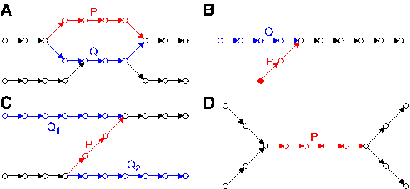
Topology of selected features within a de Bruijn graph. The red h-path, P, is the current h-path under consideration for deletion (tip removal, chimeric h-path removal) or projection to another path (bulge corremoval). The blue path(s), Q, are alternative paths. Note that other factors such as lengths and coverage are considered in addition to topology, and that the graphs continue past the regions shown. (A) A potential bulge. Q may contain hubs within it, though P does not. (B) A potential tip; h-path P starts or ends at a vertex of total degree 1 (represented as solid), and there is an alternative h-path Q. (C) A potential chimeric h-path. There must be alternative h-paths Q₁, Q₂ both for the entrance and the exit to P. (D) h-path is a repeat. Note that P starts with a vertex of outdegree one and ends with a vertex of indegree one and has no alternative h-path. These degree conditions differentiate it from (A,B,C).

SPAdes improves detection of these structures based on graph topology and the length and coverage of the h-paths comprising them. We also improve on how these structures are removed from the graph, and on bookkeeping that allows us to backtrack how reads map to paths in the assembly graph as a result of graph simplification.

6.3. Bulge corremoval versus bulge removal

Existing assembers often use two complementary approaches to deal with errors in reads: error correction in reads (Pevzner et al., 2001; Chaisson and Pevzner, 2008; Kelley et al., 2010; Ilie et al., 2010; Medvedev et al., 2011b) and bulge/bubble removal in de Bruijn graphs (Pevzner et al., 2004; Chaisson and Pevzner, 2008; Zerbino and Birney, 2008; Butler et al., 2008; Simpson et al., 2009; Li et al., 2010). Note the surprising contrast between these two approaches, both aimed at the same goal: the former approach corrects rather than removes erroneous k-mers in reads, while the latter approach removes rather than corrects erroneous k-mers in de Bruijn graphs. Removal (rather than correction) of bulges leads to deterioration of assemblies, since important information (particularly in the case of SCS) may be lost. SPAdes, unlike other NGS assemblers, records information about removed edges from bulges for later use before discarding them. We thus call this procedure “bulge correction and removal” (or bulge corremoval).

SPAdes uses the following algorithm for bulge corremoval. Paths P and Q connecting the same hubs form a simple bulge if (i) P is an h-path and (ii) the lengths of P and Q are small and similar. Note that Q is permitted to have intermediate vertices that are hubs, so it is not necessarily an h-path. Given a simple bulge formed by P and Q, SPAdes maps every edge a in P to an edge projection(a) in Q, Afterwards, it removes P from the graph. SPAdes further increases the coverage of Q to reflect the coverage of the corrected h-path P. See Section 8.4 for exact definitions of “small,” “similar,” and “projection(a).”

SPAdes maintains a data structure (see Section 8.6) allowing one to backtrack all bulge corremovals. This is used in later stages of SPAdes to map reads to the assembly graph. For example, in Stage 2, SPAdes may correct a biedge (a|b, d) associated with an erroneous edge a by changing it into the more reliable biedge (a′|b, d) (where a was replaced by a′ through a series of projections), thus preserving (rather than removing) information about distance estimates contributed by read-pairs.

Additional conditions for removing bulges, tips, and chimeric h-paths are given in Section 8.

6.4. Gradual h-path removal

Velvet and some other assemblers use a fixed coverage cutoff threshold for h-paths in the de Bruijn graph to prune out low-coverage (and likely erroneous) h-paths. This operation dramatically reduces the complexity of the underlying de Bruijn graph and makes these algorithms practical. Since SCS projects have highly variable coverage, a fixed coverage cutoff either prevents assembly of a substantial portion of the genome or fails to cut off a significant number of erroneous h-paths. Indeed, while a short low-coverage h-path in a de Bruijn graph may appear to be a good candidate for removal if the coverage is uniform, it may represent a correct path from a low coverage region in SCS.

To deal with this problem, Chitsaz et al. (2011) proposed a specific scheduling of h-path removals that uses a progressively increasing coverage threshold. To figure out whether a low-coverage h-path is correct, E+V-SC removes some other h-paths with even lower coverage first and checks whether the h-path of interest merges into a longer h-path with an increased average coverage. This “rescuing” of lower coverage paths by higher coverage paths is a feature of SCS, since low-coverage regions are often followed by high-coverage regions.

Inspired by this approach, we implemented the even more careful gradual h-path removal strategy to improve on the algorithm from Chitsaz et al. (2011) in several respects. First, unlike E+V-SC, SPAdes iterates through the list of all h-paths in increasing order of coverage (for bulge corremoval and chimeric h-path removal) or increasing order of length (for tip removal), and updates this list as h-paths are deleted or projected (instead of deleting all edges with coverage below some threshold simultaneously as in Chitsaz et al. [2011]). This allows SPAdes to “rescue” more h-paths in the graph. Second, at some points in this process, we suspend it to run only bulge corremovals, trying to process as many simple bulges as possible. Unlike a deletion of an h-path, projection of a simple bulge is a “safer” operation because it always preserves an alternative path (of similar length) in the graph, thus allowing reads to be remapped contiguously. After a series of projections, the final contigs will correspond to the paths with highest coverage in this process. Third, SPAdes introduces an important additional restriction on h-paths that are removed that ensures that no new sources/sinks are introduced to the graph: an h-path is deleted (in chimeric h-path removal) or projected (in bulge corremoval) only if its start vertex has at least two outgoing edges and its end vertex has at least two incoming edges. (For tip removal, this only applies to the hub that is not a source or sink.) This topological condition helps to eliminate low coverage h-paths arising from sequencing errors and chimeric reads (elevated in SCS), while preserving h-paths arising from repeats (Fig. 5D). See Section 8 for additional details.

6.5. Review of all stages of SPAdes

We now briefly review all stages of SPAdes. In Stage 1, given a set of bireads, denoted Bireads, SPAdes constructs the (multisized) assembly graph while maintaining data structures to map the original reads to the assembly graph. In Stage 2, we compute A(H(B(Bireads))) to generate the set of adjusted h-biedges. In Stage 3, we use the resulting accurate h-biedges for the paired assembly graph construction. In Stage 4, we output the contigs of the paired assembly graph.

7. Results

7.1. Assembly datasets

We used three datasets from Chitsaz et al. (2011). A single E. coli cell and a single marine cell (Deltaproteobacterum SAR324) were isolated by micromanipulation as described in Ishoey et al. (2008). Paired-end libraries were generated on an Illumina Genome Analyzer IIx from MDA-amplified single-cell DNA and from standard (multicell) genomic DNA prepared from cultured E. coli. We call these datasets SAR324, ECOLI-SC, and ECOLI-MC. ECOLI-SC and ECOLI-MC are called “E. coli lane 1” and “E. coli lane normal” in Chitsaz et al. (2011). They consist of 100 bp paired-end reads with average insert sizes 266 bp for ECOLI-SC, 215 bp for ECOLI-MC, and 240 bp for SAR324. Both E. coli datasets have 600 × coverage.

7.2. How accurate are the distance estimates for h-biedges?

The E. coli genome defines a walk in the assembly graph and a sequence of h-edges \documentclass{aastex}\usepackage{amsbsy}\usepackage{amsfonts}\usepackage{amssymb}\usepackage{bm}\usepackage{mathrsfs}\usepackage{pifont}\usepackage{stmaryrd}\usepackage{textcomp}\usepackage{portland, xspace}\usepackage{amsmath, amsxtra}\pagestyle{empty}\DeclareMathSizes{10}{9}{7}{6}\begin{document} $$\alpha_1, \ldots, \alpha_n$$ \end{document} . We define Gap_i as the length of a gap between path(α_i) and path(α_i₊₁). For most h-edges we actually have Gap_i = 0 (i.e., there is no gap between path(α_i) and path(α_i₊₁); in other words, path(α_i) ends at the same hub where path(α_i₊₁) starts) but ≈ 5% of h-edges have Gap_i > 0 in the ECOLI-MC dataset. We further define \documentclass{aastex}\usepackage{amsbsy}\usepackage{amsfonts}\usepackage{amssymb}\usepackage{bm}\usepackage{mathrsfs}\usepackage{pifont}\usepackage{stmaryrd}\usepackage{textcomp}\usepackage{portland, xspace}\usepackage{amsmath, amsxtra}\pagestyle{empty}\DeclareMathSizes{10}{9}{7}{6}\begin{document} $$D_{ij} = \sum\nolimits_{m = i}^{j - 1} \mid \textsc{path} (\alpha_m) \mid + \textsc{Gap}_m$$ \end{document} as the distance between the starting points of edges α_i and α_j in this walk (accounting for gaps). These distances define true h-biedges (α_i|α_j, D_ij), and we limit our attention to true h-biedges that are d-bounded (e.g., d = 166 ± 56 for the ECOLI-SC dataset).

Given a set of correct h-biedges, HBE, one can construct the h-biedge graph as described above. In practice, the set HBE is unknown and is approximated from the h-biedge histograms, resulting in the set HBE′. Below we demonstrate that HBE′ approximates the set of true h-biedges HBE well.

An h-biedge in HBE (resp., HBE′) is called a false negative (resp., false positive) if it is not present in HBE′ (resp., HBE). The false positive (negative) rate is defined as the ratio of number of false positives (negatives) to number of h-biedges in HBE′ (HBE). The false positive and false negative rates are 0.8% and 3% for the ECOLI-MC dataset and 7% and 0.7% for the ECOLI-SC dataset. Thus, SPAdes derives extremely accurate distance estimates, making the PDBG approach practical.

7.3. Benchmarking SPAdes

We benchmarked seven assemblers on three datasets (ECOLI-SC, ECOLI-MC, and SAR324). The assemblers are EULER-SR (Chaisson and Pevzner, 2008), IDBA (Peng et al., 2010), SOAPdenovo (Li et al., 2010), Velvet (Zerbino and Birney, 2008), Velvet-SC (Chitsaz et al., 2011), E+V-;SC (Chitsaz et al., 2011), and SPAdes (with and without using paired-read information). To provide unbiased benchmarking, we used the assembly evaluation tool Plantagora (http://www.plantagora.org). See Table 1.

Table 1.

Comparison of Assemblies for Single-Cell (ECOLI-SC) and Standard (ECOLI-MC) Datasets

Assembler ^a	# contigs	N50 (bp)	Largest (bp) ^b	Total (bp) ^c	Covered (%) ^d	MA ^e	MM ^f	CG ^g
Single-cell E. coli (ECOLI-SC)
EULER-SR	1344	26662	126616	4369634	87.8	21	11.0	3457
SOAPdenovo	1240	18468	87533	4237595	82.5	13	99.5	3059
Velvet	428	22648	132865	3533351	75.8	2	1.9	3117
Velvet-SC	872	19791	121367	4589603	93.8	2	1.9	3654
E+ V−SC	501	32051	132865	4570583	93.8	2	6.7	3809
SPAdes-single	1164	42492	166117	4781576	96.1	1	6.2	3888
SPAdes	1024	49623	177944	4790509	96.1	1	5.2	3911
Normal multicell sample of E. coli (ECOLI-MC)
EULER-SR	295	110153	221409	4598020	99.5	10	5.2	4232
IDBA	191	50818	164392	4566786	99.5	4	1.0	4201
SOAPdenovo	192	62512	172567	4529677	97.7	1	26.1	4141
Velvet	198	78602	196677	4570131	99.9	4	1.2	4223
Velvet-SC	350	52522	166115	4571760	99.9	0	1.3	4165
E+V-SC	339	54856	166115	4571406	99.9	0	2.9	4172
SPAdes-single	445	59666	166117	4578486	99.9	0	0.7	4246
SPAdes	195	86590	222950	4608505	99.9	2	3.7	4268

The best assembler by each criteria is indicated in bold. EULER-SR 2.0.1, Velvet 0.7.60, Velvet-SC, and E+V-SC were run with vertex size 55. SOAPdenovo 1.0.4 was run with vertex size 27–31. IDBA was run in its default iterative mode; IDBA crashed on ECOLI-SC, so IDBA results are only shown for ECOLI-MC. SPAdes-single refers to SPAdes without Stages 2 and 3, for comparison with E+V-SC, which does not use read-pair information. SPAdes and SPAdes-single iterated over edge sizes k = 22,34,56. Statistics in this table differ slightly from statistics presented in Chitsaz et al. (2011) due to the specific criteria used in Plantagora.

Length of the largest contig without a misassembly.

The total assembly size may increase (and in some cases exceeds the genome size) due to contaminants (see Chitsaz et al. (2011)), misassembled contigs, repeats, and hubs that contribute to multiple contigs. The percentage of the E. coli genome covered filters out these issues.

Percent of genome covered is the ratio of total number of aligned bases in the assembly to the genome size.

MA: Misassemblies are locations on an assembled contig where the left flanking sequence aligns over 1 kb away from the right flanking sequence on the reference.

MM: Mismatch (substitution) error rate per 100 kbp is measured in the correctly assembled contigs.

CG: Complete genes out of 4,324 genes annotated elsewhere (http://www.ecogene.org).

Table 1 illustrates that SPAdes compares well to other assemblers on multicell and, particularly, single-cell datasets. SPAdes assembled ≈ 96.1% of the E. coli genome from the ECOLI-SC dataset, with an N50 of 49623 bp and a single misassembly. E+V-SC assembled ≈ 93.8% of the E. coli genome with an N50 of 32051 and two misassemblies. SPAdes captured ≈ 100 more E. coli genes than E+V-SC, ≈800 more than Velvet, and ≈ 900 more than SOAPdenovo.

On the ECOLI-MC dataset, the EULER-SR assembly featured the largest N50 (110,153 bp) but was compromised by 10 misassemblies. All other assemblers generated a small number of misassembled contigs, ranging from 4 (IDBA and Velvet) to 0 (Velvet-SC, E+V-SC, and SPAdes-single reads). SPAdes and Velvet also had larger N50 (86,590 and 78,602 bp) than other assemblers except for EULER-SR. All assemblers but SOAPdenovo produced nearly 100% coverage of the genome. Table 1 reveals that the substitution error rate ranges over an order of magnitude for different assemblers, with Velvet (for ECOLI-SC) and SPAdes-single reads (for ECOLI-MC) the most accurate.

We further compared E+V-SC and SPAdes on the SAR324 dataset. SPAdes assembled contigs totaling 5,129,304 bp (vs. 4,255,983 bp for E+V-SC) and an N50 of 75,366 bp (as compared to 30,293 bp for E+V-SC). Since the complete genome of Deltaproteobacterium SAR324 is unknown, we used long ORFs to estimate the number of genes longer than 600 bp, as a proxy for assembly quality (see Chitsaz et al. (2011)). There are 2603 long ORFs in the SPAdes assembly versus 2377 for E+V-SC.

7.4. Running time and memory requirements of SPAdes

Since this paper focuses on assembly (rather than error correction), below we focus on time and memory requirements of SPAdes on the ECOLI-SC reads corrected by the modified Hammer.

The running time of Stage 1 is roughly proportional to the number of iterations in the construction of multisized assembly graph. We used three iterations (k = 22, 34, 56). The time per iteration varied between 30 to 40 minutes, slightly exceeding the running time for Velvet. Stage 2 (k-bimer adjustment) took 42 minutes. Stage 3 (paired assembly graph) took 9 minutes. Stage 4 (outputting contigs) took under a minute. The total time was approximately 3 hours. Peak memory was 1.5 Gb. All benchmarking was done on a 32 CPU (Intel Xeon X7560 2.27GHz) computer.

8. Additional Details on Assembly Graph Construction

8.1. Double strandedness

To account for double-strandedness, we assemble all reads and their reverse complements together. Every edge in the graph has a reverse complementary edge, although a small number of edges may be their own reverse complement. These dual pairs of edges are kept in sync through all graph transformations.

8.2. Tip removal

Errors in the start or end of a read may lead to a chain of stray edges protruding from the assembly graph but not connecting to other reads; this is called a tip (Fig. 5B). To determine if an h-path P from hub u to hub v is a tip, we consider its topology, length, and coverage:

• Topologically, an h-path that starts with a source vertex u of outdegree 1 or ends in a sink vertex v of indegree 1 may be a tip if there is an alternative h-path Q connected to the other end. If u is a source of outdegree 1 and v has indegree at least 2, one of the other h-paths ending at v (usually there is just one other) is chosen as the alternative h-path Q. Similarly, if v is a sink of indegree 1 and u has outdegree at least 2, one of the other h-paths starting at u is chosen as the alternative h-path Q.

• The length of P must be below a specified threshold, usually based on read length. For Illumina reads of length 100, we use a maximum tip length of 100. This filters out stray h-paths from bad read ends while retaining long contigs that terminate in a source or sink.

• There are two coverage thresholds, one absolute, the other relative. The average coverage of P must be below a specified threshold; we used ∞ for the datasets in this paper to disable it. The ratio of the coverage of P divided by the coverage of Q must be below a threshold; we used ∞ for the ECOLI-SC dataset to disable it, and 2.5 for ECOLI-MC.

SPAdes iterates through all h-paths of the graph in order of increasing length (terminating at the maximum tip length threshold). an h-path satisfying the above criteria to be a tip (short, has an alternative h-path, and satisfies the coverage thresholds) will be deleted from the graph. When it's deleted, the hub to which it was joined may become a vertex with indegree 1 and outdegree 1, requiring us to recompute the h-paths in that portion of the graph. As with other graph simplification procedures, we update the list of h-paths on the spot. This allows us to remove all tips from the graph in one pass, while removing as few nucleotides as possible.

8.3. Gradual chimeric h-path removal

Chimeric h-paths arise from chimeric reads and from chance short overlaps between reads.

We use a variety of tests to determine if an h-path P from hub u to hub v may be chimeric. Basic gradual h-path removal considers three criteria:

• Topologically, an h-path may be chimeric if outdegree(u) ≥ 2 and indegree(v) ≤ 2.

• The length of P must be below a specified threshold. For k = 56, we used maximum path length 150.

• The coverage should be below a threshold, based on the library. We used 30 for ECOLI-SC and 50 for ECOLI-MC.

Since coverage varies widely within SCS datasets, some chimeric junctions may be amplified in the reads. We thus developed additional heuristics to delete some chimeric junctions with high coverage, based only on topology and length rather than coverage. (However, there may still be chimeric junctions not detected by these heuristics.) Most chimeric h-paths are observed to be smaller than ≈ k + 10. Bacterial genomes typically have a small number of long repeats (several kb long). As an example, consider a vertex v with two incoming h-paths (P₀ of length ≈ k and P₁ of length ≈ 3k), and one outgoing h-path (P₂ of length several thousand bases); these are the only h-paths incident with v. If all three h-paths are correct, then P₂ must be a long repeat of multiplicity at least 2. However, P₀ satisfies the topology and length conditions for a chimeric h-path, and it is more likely that P₀ is chimeric but the chimeric junction was amplified, so we delete P₀.

8.4. Gradual bulge corremoval

Paths P and Q connecting the same hubs form a simple bulge if (i) P is an h-path and (ii) the lengths of P and Q are small and similar. Note that Q may have additional hubs along the path, so Q is a path but not necessarily an h-path.

By default, the length of P (and Q) is small if it is at most 150 and the lengths |P|,|Q| are similar if either \documentclass{aastex}\usepackage{amsbsy}\usepackage{amsfonts}\usepackage{amssymb}\usepackage{bm}\usepackage{mathrsfs}\usepackage{pifont}\usepackage{stmaryrd}\usepackage{textcomp}\usepackage{portland, xspace}\usepackage{amsmath, amsxtra}\pagestyle{empty}\DeclareMathSizes{10}{9}{7}{6}\begin{document} $$\big| \mid P \mid - \mid Q \mid \big| \leq 3$$ \end{document} or \documentclass{aastex}\usepackage{amsbsy}\usepackage{amsfonts}\usepackage{amssymb}\usepackage{bm}\usepackage{mathrsfs}\usepackage{pifont}\usepackage{stmaryrd}\usepackage{textcomp}\usepackage{portland, xspace}\usepackage{amsmath, amsxtra}\pagestyle{empty}\DeclareMathSizes{10}{9}{7}{6}\begin{document} $$\big| \mid P \mid - \mid Q \mid \big| \leq 0.05 \mid P \mid$$ \end{document} . The numeric values are parameters that can be changed.

To correct a bulge, SPAdes removes path P from the graph, and substitutes each edge a of P by an edge projection(a) in Q. If a is at offset i in P, then projection(a) is in Q at offset \documentclass{aastex}\usepackage{amsbsy}\usepackage{amsfonts}\usepackage{amssymb}\usepackage{bm}\usepackage{mathrsfs}\usepackage{pifont}\usepackage{stmaryrd}\usepackage{textcomp}\usepackage{portland, xspace}\usepackage{amsmath, amsxtra}\pagestyle{empty}\DeclareMathSizes{10}{9}{7}{6}\begin{document} \begin{align*} 1 + \textsc{round} \left(\frac {(i - 1) \cdot (\mid Q \mid - 1)} {\mid P \mid - 1} \right). \end{align*} \end{document}

8.5. Isolated h-path removal

After all other graph simplification procedures, we remove isolated h-paths with length below 200.

8.6. Backtracking edges relocated during graph simplification

Although the graph simplification algorithm is universal, bookkeeping operations are performed that allow us to map reads back to their positions in the assembly graph after graph simplification. This is used in Stage 2 to map bireads to the simplified graph, and may be output in Stage 4 for downstream applications. The bookkeeping details presented here are specific for assembling a de Bruijn graph from reads and simplifying the graph. The details may change for other A-Bruijn graph applications.

For a de Bruijn graph with k-mer edges, the graph editing operations can be described as either projecting one k-mer x onto another, y, or deleting x. We keep track of this through functions Map(x) and Map*(x) on k-mers. Let S be the set of all k-mers (edge labels) in the de Bruijn graph.

• Initially, we set Map(x) = x for all \documentclass{aastex}\usepackage{amsbsy}\usepackage{amsfonts}\usepackage{amssymb}\usepackage{bm}\usepackage{mathrsfs}\usepackage{pifont}\usepackage{stmaryrd}\usepackage{textcomp}\usepackage{portland, xspace}\usepackage{amsmath, amsxtra}\pagestyle{empty}\DeclareMathSizes{10}{9}{7}{6}\begin{document} $$x \in S$$ \end{document} .

• To project edge x to edge y, where y has not yet been remapped (that is, Map(y) = y), we set Map(x) = y.

• To delete edge x, we set Map(x) = DEL, which is a code indicating deletion.

• A series of projections during graph simplification may result in Map(x) = y, Map(y) = z, and so on. We define \documentclass{aastex}\usepackage{amsbsy}\usepackage{amsfonts}\usepackage{amssymb}\usepackage{bm}\usepackage{mathrsfs}\usepackage{pifont}\usepackage{stmaryrd}\usepackage{textcomp}\usepackage{portland, xspace}\usepackage{amsmath, amsxtra}\pagestyle{empty}\DeclareMathSizes{10}{9}{7}{6}\begin{document} $$\textsc{MAP}^* (x) = \textsc{MAP} (\textsc{MAP} (\ldots (x)))$$ \end{document} , where we repeatedly apply the Map function until the value stabilizes. We directly implement Map* (rather than Map) by using a union-find data structure.

While the presentation in this article used edges representing k-mers, many steps in the assembler are implemented in terms of condensed edges representing sequences of varying length. Each h-path in the assembly graph (consisting of many vertices and edges) is represented as one condensed edge. As the graph is simplified, some condensed edges need to be combined into longer condensed edges.

The “universal graph” properties associated with condensed edge e include a numeric edge ID; the edge ID of the conjugate edge (for double-stranded assembly); the length (number of edges in the standard de Bruijn graph that were condensed to give this one edge; this is equivalent to length in nucleotides, ignoring the length of the terminal vertex); average coverage along e; and h-biedge histograms.

Each condensed edge e has a numeric edge ID and a string EdgeString(e) of the DNA sequence along the edge. Note that no k-mer is ever contained in more than one condensed edge. Bookkeeping with the condensed edge representation of the assembly graph is implemented as follows.

(1) Build the de Bruijn graph and compute the set S of all k-mers.

(2) Build the condensed de Bruijn graph. While forming the h-paths, we create bookkeeping structures Map/Map*, EdgeIndex, and EdgeString:

• Define Map(x) = x for all \documentclass{aastex}\usepackage{amsbsy}\usepackage{amsfonts}\usepackage{amssymb}\usepackage{bm}\usepackage{mathrsfs}\usepackage{pifont}\usepackage{stmaryrd}\usepackage{textcomp}\usepackage{portland, xspace}\usepackage{amsmath, amsxtra}\pagestyle{empty}\DeclareMathSizes{10}{9}{7}{6}\begin{document} $$x \in S$$ \end{document} .

• Define EdgeIndex(x) = (e, i) where e is the condensed edge containing x, and i is the offset of x along it.

• Set EdgeString(e) to the nucleotide sequence on condensed edge e.

(3) For bulge corremoval, k-mer x is projected to k-mer y by setting Map(x) = y.

(4) Condensed edge e is deleted by setting EdgeIndex(x) = (DEL, 0) for all k-mers x in EdgeString(e).

(5) After projection and deletion operations, vertices previously classified as hubs may change to non-hubs (indegree(v) = outdegree(v) = 1), requiring us to combine a sequence of condensed edges into one condensed edge. To recombine a path comprised of segments \documentclass{aastex}\usepackage{amsbsy}\usepackage{amsfonts}\usepackage{amssymb}\usepackage{bm}\usepackage{mathrsfs}\usepackage{pifont}\usepackage{stmaryrd}\usepackage{textcomp}\usepackage{portland, xspace}\usepackage{amsmath, amsxtra}\pagestyle{empty}\DeclareMathSizes{10}{9}{7}{6}\begin{document} $$e_1, \ldots, e_n$$ \end{document} into a single new condensed edge e:

• For \documentclass{aastex}\usepackage{amsbsy}\usepackage{amsfonts}\usepackage{amssymb}\usepackage{bm}\usepackage{mathrsfs}\usepackage{pifont}\usepackage{stmaryrd}\usepackage{textcomp}\usepackage{portland, xspace}\usepackage{amsmath, amsxtra}\pagestyle{empty}\DeclareMathSizes{10}{9}{7}{6}\begin{document} $$j = 1, \ldots, n - 1$$ \end{document} , note that End(e_j) and Start(e_j₊₁) are the same vertex and represent the same (k − 1)-mer. This vertex was previously a hub but is no longer a hub.

• Define EdgeString(e) by concatenating \documentclass{aastex}\usepackage{amsbsy}\usepackage{amsfonts}\usepackage{amssymb}\usepackage{bm}\usepackage{mathrsfs}\usepackage{pifont}\usepackage{stmaryrd}\usepackage{textcomp}\usepackage{portland, xspace}\usepackage{amsmath, amsxtra}\pagestyle{empty}\DeclareMathSizes{10}{9}{7}{6}\begin{document} \begin{align*} \textsc{EdgeString} (e_1), \ldots, \textsc{EdgeString} (e_n) \end{align*} \end{document}

but overlap the final (k − 1)-mer of each string with the initial (k − 1)-mer of the next string.

• For each k-mer x in EdgeString(e), set EdgeIndex(x) to (e, i), where i is the offset of x on e.

(6) After all graph simplifications, \documentclass{aastex}\usepackage{amsbsy}\usepackage{amsfonts}\usepackage{amssymb}\usepackage{bm}\usepackage{mathrsfs}\usepackage{pifont}\usepackage{stmaryrd}\usepackage{textcomp}\usepackage{portland, xspace}\usepackage{amsmath, amsxtra}\pagestyle{empty}\DeclareMathSizes{10}{9}{7}{6}\begin{document} $$x \in S$$ \end{document} may be located in the graph as follows:

• Compute Map*(x) = y.

• Compute EdgeIndex(y) = (e, i).

• If y is deleted (e = DEL) then return that x is deleted.

• Otherwise, return that x is represented by k-mer y, located on edge e at offset i.

After graph simplification, we can locate where any read is represented in the graph by breaking it into its k-mers and applying the Map* and EdgeIndex functions. The positions of the k-mers are sufficient to compute the h-biedge histograms described in Stage 2. For downstream applications, a more detailed alignment of reads to contigs may be required. Before graph simplification, the list of k-mers in a read maps to a sequence of edges forming a path in the de Bruijn graph. After graph simplification, there may be some disruptions in continuity of the path, due to deletion of edges and due to bulge corremovals involving paths of slightly different lengths (arising from indels). However, the approximate positions in the graph are sufficient to realign the read to the contigs (EdgeString of each condensed edge) in the graph.

9. Example of Constructing Paired Assembly Graph

We illustrate the construction of the paired assembly graph in Figure 4. We treat the case of all reads at a fixed genomic distance. This small example illustrates the definitions, rather than covering all the complexities that may arise.

Read-pairs sampled from a circular 24 bp genome \documentclass{aastex}\usepackage{amsbsy}\usepackage{amsfonts}\usepackage{amssymb}\usepackage{bm}\usepackage{mathrsfs}\usepackage{pifont}\usepackage{stmaryrd}\usepackage{textcomp}\usepackage{portland, xspace}\usepackage{amsmath, amsxtra}\pagestyle{empty}\DeclareMathSizes{10}{9}{7}{6}\begin{document} \begin{align*} \textsc{Genome} = {\rm ACGTCAAGTTCTGACGTGGGTTCT} \end{align*} \end{document}

form a set of single reads referred to as Reads. We take all pairs of reads (bireads) of length 6 with insert size 11; this translates into pairs of reads of length 6 whose starting positions are separated by d = 11 − 6 = 5. In the general case, distances would vary in each biread, and the reads in a biread would not overlap, but such an example is too large to show.

For k = 4, read ACGTCA contributes vertices ACG, CGT, GTC, TCA and edges ACGT, CGTC, GTCA to the de Bruijn graph DB(Reads, 4) (Fig. 4A).

The de Bruijn graph DB(Reads, 4) has four hubs (ACG, CGT, GTT, and TCT) and six h-paths \documentclass{aastex}\usepackage{amsbsy}\usepackage{amsfonts}\usepackage{amssymb}\usepackage{bm}\usepackage{mathrsfs}\usepackage{pifont}\usepackage{stmaryrd}\usepackage{textcomp}\usepackage{portland, xspace}\usepackage{amsmath, amsxtra}\pagestyle{empty}\DeclareMathSizes{10}{9}{7}{6}\begin{document} $$P_1, \ldots, P_6$$ \end{document} , with path lengths \documentclass{aastex}\usepackage{amsbsy}\usepackage{amsfonts}\usepackage{amssymb}\usepackage{bm}\usepackage{mathrsfs}\usepackage{pifont}\usepackage{stmaryrd}\usepackage{textcomp}\usepackage{portland, xspace}\usepackage{amsmath, amsxtra}\pagestyle{empty}\DeclareMathSizes{10}{9}{7}{6}\begin{document} $$1, \ldots, 6$$ \end{document} respectively. Note that path length is measured in edges; the string spelled by path P_i is k − 1 symbols longer than the path length. The h-edge of path P_i is denoted α_i. The cycle C in DB(Reads, 4) that spells Genome passes through the h-paths in order P₁, P₆, P₂, P₄, P₁, P₅, P₂, P₃. Note that P₁ and P₂ represent repeats (ACGT and GTTCT, respectively); these arise because the de Bruijn graph glues together repeats of size at least k − 1 = 3.

Each biread from Genome contributes information about genomic distances that is collected on h-biedges. For example, the biread (ACGTCA, AAGTTC) contributes 4-bimers (ACGT|AAGT, 5), (CGTC|AGTT, 5), (GTCA|GTTC, 5) to the paired assembly graph, which in turn yield h-biedges (α₁|α₆, 1), (α₆|α₆, 0), (α₆|α₂, 6). In Figure 4B, 13 h-biedges constructed from all bireads are shown as rectangles numbered as \documentclass{aastex}\usepackage{amsbsy}\usepackage{amsfonts}\usepackage{amssymb}\usepackage{bm}\usepackage{mathrsfs}\usepackage{pifont}\usepackage{stmaryrd}\usepackage{textcomp}\usepackage{portland, xspace}\usepackage{amsmath, amsxtra}\pagestyle{empty}\DeclareMathSizes{10}{9}{7}{6}\begin{document} $$R_1, \ldots, R_{13}$$ \end{document} . For the reader's convenience, these are listed and numbered in the order traversed by the cycle C, although it is not known in advance. Since this example has fixed distance d = 5, distinct values of D let us separate different instances of the same pairs α_i, α_j (in this case, separating (α₂|α₁, 5) and (α₂|α₁, 6)).

The h-biedge (α₆|α₂, 6) results in rectangle R₃ (Fig. 4C) with sides P₆ and P₂ and 45^° line segment y = x + (d − 6) = x + (5 − 6) = x − 1 from point (1, 0) to (3, 2). Point (1, 0) in R₁₃ is labeled by bivertex (GTC|GTT) formed by vertex 1 in path P₆ and vertex 0 in path P₂. Formally, it is computed as Start(First(α₆|α₂, 6)) = Start(CGTC|GTTC) = (CGT|GTT). Point (3, 2) in R₃ is labeled by bivertex (CAA|TCT) formed by vertex 3 in path P₆ and vertex 2 in path P₂. Formally, it is computed as End(Last(α₆|α₂, 6)) = End(AGTT|TTCT) = (GTT|TCT).

Applying gluing rule H2 to the 26 bivertices arising from these 13 rectangles (h-biedges) forms a single cycle that reconstructs Genome. The resulting paired assembly graph is comprised of the blue edges (45^° segments within rectangles) and blue vertices (labeled by bivertices); the dotted red lines show vertices that are pasted together to form a single vertex. Edges (resp., vertices) of the paired assembly graph are labeled by h-biedges (resp., bivertices) of G.

In Figure 4C, all possible h-biedges are represented as rectangles on a 24 × 24 grid, with x- and y-axes corresponding to Genome. In this example, the distance between reads within read-pairs is d = 5. The blue 45^° line y = x + d crosses 13 rectangles revealed by read-pairs; since the genome is circular, the 45^° line is broken into two segments.

10. Universal Genome Assembly

In this section, we present an abstraction for assembly graphs (and other A-Bruijn graphs) for which edge labels (e.g., substrings of the genome) are hidden and only lengths and/or coverages of the edges are given. For the sake of simplicity, we address the case of a unichromosomal circular genome corresponding to a cycle in the graph. The goal is reconstruct the cycle (without using edge labels) and afterwards “translate” this cycle into a genome (by recalling edge labels).

A weighted directed graph G = (V, A, ℓ) consists of the set of vertices V, the set of (directed) edges A ⊂ V × V, and a function \documentclass{aastex}\usepackage{amsbsy}\usepackage{amsfonts}\usepackage{amssymb}\usepackage{bm}\usepackage{mathrsfs}\usepackage{pifont}\usepackage{stmaryrd}\usepackage{textcomp}\usepackage{portland, xspace}\usepackage{amsmath, amsxtra}\pagestyle{empty}\DeclareMathSizes{10}{9}{7}{6}\begin{document} $$\ell : A \rightarrow {\mathbb N}$$ \end{document} specifying the length (weight) of each edge. We extend function ℓ to measure the length of any path/cycle in G as the total length of its edges.

Definition 1. The distance d_G(u, v) between vertices \documentclass{aastex}\usepackage{amsbsy}\usepackage{amsfonts}\usepackage{amssymb}\usepackage{bm}\usepackage{mathrsfs}\usepackage{pifont}\usepackage{stmaryrd}\usepackage{textcomp}\usepackage{portland, xspace}\usepackage{amsmath, amsxtra}\pagestyle{empty}\DeclareMathSizes{10}{9}{7}{6}\begin{document} $$u, v \in V$$ \end{document} is the length of a shortest (directed) path starting at u and ending at v. If there is no such path, we let d_G(u, v) = ∞.

Definition 2. The distance d_G(a, b) between edges a = (u₁, u₂) and b = (v₁, v₂) is ℓ(u₁, u₂) + d_G(u₂, v₁) + ℓ(v₁, v₂) (the length of a shortest path starting at a and ending at b).

Definition 3. The distance d_G(a, v) between an edge a = (u₁, u₂) and a vertex v is defined as ℓ(u₁, u₂) + d_G(u₂,v). Similarly, d_G(v, a) = d_G(v, u₁) + ℓ(u₁, u₂).

Notice that a vertex/edge may appear multiple times in a path/cycle. Hence, here we distinguish vertices/edges and their instances. Depending on the context, we will treat a path/cycle as a linear/cyclic sequence of vertex/edge instances visited by the path/cycle in order.

Definition 4. For a cycle C and any vertex/edge instances \documentclass{aastex}\usepackage{amsbsy}\usepackage{amsfonts}\usepackage{amssymb}\usepackage{bm}\usepackage{mathrsfs}\usepackage{pifont}\usepackage{stmaryrd}\usepackage{textcomp}\usepackage{portland, xspace}\usepackage{amsmath, amsxtra}\pagestyle{empty}\DeclareMathSizes{10}{9}{7}{6}\begin{document} $$x, y \in C$$ \end{document} , we define

• the subpath Subpath_C(x, y) of C, starting at x and ending at y; if there is no such subpath, Subpath_C(x, y) = ∅

• the C-distance d_C(x, y) as the length of Subpath_C(x, y); if there is no such subpath, d_C(x, y) = ∞ .

Let β,γ ≥ 0 be parameters specifying constraints on parallel paths and bulges in graph G.

Definition 5. A cycle C′ is called (β, γ)-embedded into a cycle C (denoted C′ ⊂ _β,γC) if for every edge \documentclass{aastex}\usepackage{amsbsy}\usepackage{amsfonts}\usepackage{amssymb}\usepackage{bm}\usepackage{mathrsfs}\usepackage{pifont}\usepackage{stmaryrd}\usepackage{textcomp}\usepackage{portland, xspace}\usepackage{amsmath, amsxtra}\pagestyle{empty}\DeclareMathSizes{10}{9}{7}{6}\begin{document} $$a \in (C^{\prime} \setminus C)$$ \end{document} , there exist two vertex instances u₁, u₂ in both C and C′ such that \documentclass{aastex}\usepackage{amsbsy}\usepackage{amsfonts}\usepackage{amssymb}\usepackage{bm}\usepackage{mathrsfs}\usepackage{pifont}\usepackage{stmaryrd}\usepackage{textcomp}\usepackage{portland, xspace}\usepackage{amsmath, amsxtra}\pagestyle{empty}\DeclareMathSizes{10}{9}{7}{6}\begin{document} $$a \in \textsc{Subpath}_{C^{\prime}} (u_1, u_2)$$ \end{document} and \documentclass{aastex}\usepackage{amsbsy}\usepackage{amsfonts}\usepackage{amssymb}\usepackage{bm}\usepackage{mathrsfs}\usepackage{pifont}\usepackage{stmaryrd}\usepackage{textcomp}\usepackage{portland, xspace}\usepackage{amsmath, amsxtra}\pagestyle{empty}\DeclareMathSizes{10}{9}{7}{6}\begin{document} \begin{align*} & \max \{d_C (u_1, u_2), d_{C^{\prime}} (u_1, u_2) \} \leq \beta, \\ & \mid d_C (u_1, u_2) - d_{C^{\prime}} (u_1, u_2) \mid \leq \gamma. \end{align*} \end{document}

Definition 6. A cycle C′ is called telescopically (β,γ)-embedded into a cycle C (denoted \documentclass{aastex}\usepackage{amsbsy}\usepackage{amsfonts}\usepackage{amssymb}\usepackage{bm}\usepackage{mathrsfs}\usepackage{pifont}\usepackage{stmaryrd}\usepackage{textcomp}\usepackage{portland, xspace}\usepackage{amsmath, amsxtra}\pagestyle{empty}\DeclareMathSizes{10}{9}{7}{6}\begin{document} $$C^{\prime} \subset_{\beta, \gamma}^* C$$ \end{document} ) if there exists a sequence of (β,γ)-embedded cycles starting with C′ and ending with C: \documentclass{aastex}\usepackage{amsbsy}\usepackage{amsfonts}\usepackage{amssymb}\usepackage{bm}\usepackage{mathrsfs}\usepackage{pifont}\usepackage{stmaryrd}\usepackage{textcomp}\usepackage{portland, xspace}\usepackage{amsmath, amsxtra}\pagestyle{empty}\DeclareMathSizes{10}{9}{7}{6}\begin{document} \begin{align*} C^{\prime} \subset_{\beta, \gamma} C_1 \subset_{\beta, \gamma} C_2 \subset_{\beta, \gamma} \cdots \subset_{\beta, \gamma} C_k \subset_{\beta, \gamma}C. \end{align*} \end{document}

The Universal Genome Assembly Problem (UGAP) can be formulated as follows.

Input.

• a weighted directed graph G = (V, A, ℓ);

• a set BE of biedges (a|b, D), where a and b are edges in G and D is the estimated genomic distance between them;

• a parameter δ ≥ 0 (maximal relative variation in distance estimates);

• parameters β, γ ≥ 0 (specifying constraints on parallel paths and bulges).

Output. A shortest cycle C in G such that

• for any edge \documentclass{aastex}\usepackage{amsbsy}\usepackage{amsfonts}\usepackage{amssymb}\usepackage{bm}\usepackage{mathrsfs}\usepackage{pifont}\usepackage{stmaryrd}\usepackage{textcomp}\usepackage{portland, xspace}\usepackage{amsmath, amsxtra}\pagestyle{empty}\DeclareMathSizes{10}{9}{7}{6}\begin{document} $$a \in A$$ \end{document} , there exists a cycle C′ such that \documentclass{aastex}\usepackage{amsbsy}\usepackage{amsfonts}\usepackage{amssymb}\usepackage{bm}\usepackage{mathrsfs}\usepackage{pifont}\usepackage{stmaryrd}\usepackage{textcomp}\usepackage{portland, xspace}\usepackage{amsmath, amsxtra}\pagestyle{empty}\DeclareMathSizes{10}{9}{7}{6}\begin{document} $$a \in C^{\prime}$$ \end{document} and \documentclass{aastex}\usepackage{amsbsy}\usepackage{amsfonts}\usepackage{amssymb}\usepackage{bm}\usepackage{mathrsfs}\usepackage{pifont}\usepackage{stmaryrd}\usepackage{textcomp}\usepackage{portland, xspace}\usepackage{amsmath, amsxtra}\pagestyle{empty}\DeclareMathSizes{10}{9}{7}{6}\begin{document} $$C^{\prime} \subset_{\beta, \gamma}^* C$$ \end{document} ;

• for any biedge \documentclass{aastex}\usepackage{amsbsy}\usepackage{amsfonts}\usepackage{amssymb}\usepackage{bm}\usepackage{mathrsfs}\usepackage{pifont}\usepackage{stmaryrd}\usepackage{textcomp}\usepackage{portland, xspace}\usepackage{amsmath, amsxtra}\pagestyle{empty}\DeclareMathSizes{10}{9}{7}{6}\begin{document} $$(a \mid b, D) \in {\rm BE}$$ \end{document} , there exists a cycle \documentclass{aastex}\usepackage{amsbsy}\usepackage{amsfonts}\usepackage{amssymb}\usepackage{bm}\usepackage{mathrsfs}\usepackage{pifont}\usepackage{stmaryrd}\usepackage{textcomp}\usepackage{portland, xspace}\usepackage{amsmath, amsxtra}\pagestyle{empty}\DeclareMathSizes{10}{9}{7}{6}\begin{document} $$C^{\prime} \subset_{\beta, \gamma}^* C$$ \end{document} having a subpath \documentclass{aastex}\usepackage{amsbsy}\usepackage{amsfonts}\usepackage{amssymb}\usepackage{bm}\usepackage{mathrsfs}\usepackage{pifont}\usepackage{stmaryrd}\usepackage{textcomp}\usepackage{portland, xspace}\usepackage{amsmath, amsxtra}\pagestyle{empty}\DeclareMathSizes{10}{9}{7}{6}\begin{document} $$\textsc{Subpath}_{C^{\prime}} (a, b)$$ \end{document} (for some instances of a and b in C′) of length in the interval D · (1 ± δ).

Below we describe some properties of an (unknown) cycle C representing a solution to the UGAP problem that naturally guides its reconstruction; the proofs are omitted.

Property 1. For every edge \documentclass{aastex}\usepackage{amsbsy}\usepackage{amsfonts}\usepackage{amssymb}\usepackage{bm}\usepackage{mathrsfs}\usepackage{pifont}\usepackage{stmaryrd}\usepackage{textcomp}\usepackage{portland, xspace}\usepackage{amsmath, amsxtra}\pagestyle{empty}\DeclareMathSizes{10}{9}{7}{6}\begin{document} $$a = (v_1, v_2) \,\notin\, C$$ \end{document} , there exist vertex instances \documentclass{aastex}\usepackage{amsbsy}\usepackage{amsfonts}\usepackage{amssymb}\usepackage{bm}\usepackage{mathrsfs}\usepackage{pifont}\usepackage{stmaryrd}\usepackage{textcomp}\usepackage{portland, xspace}\usepackage{amsmath, amsxtra}\pagestyle{empty}\DeclareMathSizes{10}{9}{7}{6}\begin{document} $$u_1, u_2 \in C$$ \end{document} such that \documentclass{aastex}\usepackage{amsbsy}\usepackage{amsfonts}\usepackage{amssymb}\usepackage{bm}\usepackage{mathrsfs}\usepackage{pifont}\usepackage{stmaryrd}\usepackage{textcomp}\usepackage{portland, xspace}\usepackage{amsmath, amsxtra}\pagestyle{empty}\DeclareMathSizes{10}{9}{7}{6}\begin{document} \begin{align*} & \max \{d_c (u_1, u_2), d_G (u_1, v_1) + \ell (v_1, v_2) + d_G (v_2, u_2) \} \leq \beta, \\ & \mid d_G (u_1, v_1) + \ell (v_1, v_2) + d_G (v_2, u_2) - d_C (u_1, u_2) \mid \leq \gamma. \end{align*} \end{document}

We define Left(a) and Right(a) as arbitrary vertex instances \documentclass{aastex}\usepackage{amsbsy}\usepackage{amsfonts}\usepackage{amssymb}\usepackage{bm}\usepackage{mathrsfs}\usepackage{pifont}\usepackage{stmaryrd}\usepackage{textcomp}\usepackage{portland, xspace}\usepackage{amsmath, amsxtra}\pagestyle{empty}\DeclareMathSizes{10}{9}{7}{6}\begin{document} $$u_1, u_2 \in C$$ \end{document} satisfying Property 1. For example, in Figure 6, if cycle C passes through edges \documentclass{aastex}\usepackage{amsbsy}\usepackage{amsfonts}\usepackage{amssymb}\usepackage{bm}\usepackage{mathrsfs}\usepackage{pifont}\usepackage{stmaryrd}\usepackage{textcomp}\usepackage{portland, xspace}\usepackage{amsmath, amsxtra}\pagestyle{empty}\DeclareMathSizes{10}{9}{7}{6}\begin{document} $$\vec{a}, \vec{b}, \vec{c}, \vec{d}, \vec{h}$$ \end{document} but not \documentclass{aastex}\usepackage{amsbsy}\usepackage{amsfonts}\usepackage{amssymb}\usepackage{bm}\usepackage{mathrsfs}\usepackage{pifont}\usepackage{stmaryrd}\usepackage{textcomp}\usepackage{portland, xspace}\usepackage{amsmath, amsxtra}\pagestyle{empty}\DeclareMathSizes{10}{9}{7}{6}\begin{document} $$\vec{e}$$ \end{document} , then for the edge \documentclass{aastex}\usepackage{amsbsy}\usepackage{amsfonts}\usepackage{amssymb}\usepackage{bm}\usepackage{mathrsfs}\usepackage{pifont}\usepackage{stmaryrd}\usepackage{textcomp}\usepackage{portland, xspace}\usepackage{amsmath, amsxtra}\pagestyle{empty}\DeclareMathSizes{10}{9}{7}{6}\begin{document} $$\vec{e}$$ \end{document} candidate vertices satisfying Property 1 would be Left( \documentclass{aastex}\usepackage{amsbsy}\usepackage{amsfonts}\usepackage{amssymb}\usepackage{bm}\usepackage{mathrsfs}\usepackage{pifont}\usepackage{stmaryrd}\usepackage{textcomp}\usepackage{portland, xspace}\usepackage{amsmath, amsxtra}\pagestyle{empty}\DeclareMathSizes{10}{9}{7}{6}\begin{document} $$\vec{e}$$ \end{document} ) = u and Right( \documentclass{aastex}\usepackage{amsbsy}\usepackage{amsfonts}\usepackage{amssymb}\usepackage{bm}\usepackage{mathrsfs}\usepackage{pifont}\usepackage{stmaryrd}\usepackage{textcomp}\usepackage{portland, xspace}\usepackage{amsmath, amsxtra}\pagestyle{empty}\DeclareMathSizes{10}{9}{7}{6}\begin{document} $$\vec{e}$$ \end{document} ) = w.

FIG. 6.

Example of parallel paths and bulges. Edges are labeled as vectors and vertices are labeled as scalars.

The second property ensures that the cycle C cannot be shortened by rerouting some of its subpaths:

Property 2. There exist no two distinct subpaths P₁, P₂ ⊂ C, both starting and ending at the same two vertices, such that \documentclass{aastex}\usepackage{amsbsy}\usepackage{amsfonts}\usepackage{amssymb}\usepackage{bm}\usepackage{mathrsfs}\usepackage{pifont}\usepackage{stmaryrd}\usepackage{textcomp}\usepackage{portland, xspace}\usepackage{amsmath, amsxtra}\pagestyle{empty}\DeclareMathSizes{10}{9}{7}{6}\begin{document} \begin{align*} \max \{\ell (P_1), \ell (P_2) \} \leq \beta \quad and \quad \mid \ell (P_1) - \ell (P_2) \mid \leq \gamma. \end{align*} \end{document}

For example, in Figure 6, if C passes through edges \documentclass{aastex}\usepackage{amsbsy}\usepackage{amsfonts}\usepackage{amssymb}\usepackage{bm}\usepackage{mathrsfs}\usepackage{pifont}\usepackage{stmaryrd}\usepackage{textcomp}\usepackage{portland, xspace}\usepackage{amsmath, amsxtra}\pagestyle{empty}\DeclareMathSizes{10}{9}{7}{6}\begin{document} $$\vec{b}, \vec{c}$$ \end{document} , as well as through \documentclass{aastex}\usepackage{amsbsy}\usepackage{amsfonts}\usepackage{amssymb}\usepackage{bm}\usepackage{mathrsfs}\usepackage{pifont}\usepackage{stmaryrd}\usepackage{textcomp}\usepackage{portland, xspace}\usepackage{amsmath, amsxtra}\pagestyle{empty}\DeclareMathSizes{10}{9}{7}{6}\begin{document} $$\vec{e}, \vec{f}$$ \end{document} , then it would violate Property 2 unless \documentclass{aastex}\usepackage{amsbsy}\usepackage{amsfonts}\usepackage{amssymb}\usepackage{bm}\usepackage{mathrsfs}\usepackage{pifont}\usepackage{stmaryrd}\usepackage{textcomp}\usepackage{portland, xspace}\usepackage{amsmath, amsxtra}\pagestyle{empty}\DeclareMathSizes{10}{9}{7}{6}\begin{document} $$\max \{\ell (\vec{b}) + \ell (\vec{c}), \ell (\vec{e}) + \ell (\vec{f}) \} > \beta$$ \end{document} or \documentclass{aastex}\usepackage{amsbsy}\usepackage{amsfonts}\usepackage{amssymb}\usepackage{bm}\usepackage{mathrsfs}\usepackage{pifont}\usepackage{stmaryrd}\usepackage{textcomp}\usepackage{portland, xspace}\usepackage{amsmath, amsxtra}\pagestyle{empty}\DeclareMathSizes{10}{9}{7}{6}\begin{document} $$\mid \ell (\vec{b}) + \ell (\vec{c}) - \ell (\vec{e}) - \ell (\vec{f}) \mid > \gamma.$$ \end{document}

The third property ensures that cycle C obeys the prescribed distances for biedges in BE:

Property 3. For any biedge \documentclass{aastex}\usepackage{amsbsy}\usepackage{amsfonts}\usepackage{amssymb}\usepackage{bm}\usepackage{mathrsfs}\usepackage{pifont}\usepackage{stmaryrd}\usepackage{textcomp}\usepackage{portland, xspace}\usepackage{amsmath, amsxtra}\pagestyle{empty}\DeclareMathSizes{10}{9}{7}{6}\begin{document} $$(a \mid b, D) \in {\rm BE}$$ \end{document} ,

• if \documentclass{aastex}\usepackage{amsbsy}\usepackage{amsfonts}\usepackage{amssymb}\usepackage{bm}\usepackage{mathrsfs}\usepackage{pifont}\usepackage{stmaryrd}\usepackage{textcomp}\usepackage{portland, xspace}\usepackage{amsmath, amsxtra}\pagestyle{empty}\DeclareMathSizes{10}{9}{7}{6}\begin{document} $$a \in C$$ \end{document} and \documentclass{aastex}\usepackage{amsbsy}\usepackage{amsfonts}\usepackage{amssymb}\usepackage{bm}\usepackage{mathrsfs}\usepackage{pifont}\usepackage{stmaryrd}\usepackage{textcomp}\usepackage{portland, xspace}\usepackage{amsmath, amsxtra}\pagestyle{empty}\DeclareMathSizes{10}{9}{7}{6}\begin{document} $$b \,\notin\, C$$ \end{document} C, then there exists an instance of a in C with \documentclass{aastex}\usepackage{amsbsy}\usepackage{amsfonts}\usepackage{amssymb}\usepackage{bm}\usepackage{mathrsfs}\usepackage{pifont}\usepackage{stmaryrd}\usepackage{textcomp}\usepackage{portland, xspace}\usepackage{amsmath, amsxtra}\pagestyle{empty}\DeclareMathSizes{10}{9}{7}{6}\begin{document} \begin{align*} \mid d_C (a, \textsc{Left} (b)) + d_G (\textsc{Left} (b), b) - D \mid \leq \delta; \end{align*} \end{document}

if \documentclass{aastex}\usepackage{amsbsy}\usepackage{amsfonts}\usepackage{amssymb}\usepackage{bm}\usepackage{mathrsfs}\usepackage{pifont}\usepackage{stmaryrd}\usepackage{textcomp}\usepackage{portland, xspace}\usepackage{amsmath, amsxtra}\pagestyle{empty}\DeclareMathSizes{10}{9}{7}{6}\begin{document} $$a \, \notin \,C$$ \end{document} and \documentclass{aastex}\usepackage{amsbsy}\usepackage{amsfonts}\usepackage{amssymb}\usepackage{bm}\usepackage{mathrsfs}\usepackage{pifont}\usepackage{stmaryrd}\usepackage{textcomp}\usepackage{portland, xspace}\usepackage{amsmath, amsxtra}\pagestyle{empty}\DeclareMathSizes{10}{9}{7}{6}\begin{document} $$b \in C$$ \end{document} , then there exists an instance of b in C with \documentclass{aastex}\usepackage{amsbsy}\usepackage{amsfonts}\usepackage{amssymb}\usepackage{bm}\usepackage{mathrsfs}\usepackage{pifont}\usepackage{stmaryrd}\usepackage{textcomp}\usepackage{portland, xspace}\usepackage{amsmath, amsxtra}\pagestyle{empty}\DeclareMathSizes{10}{9}{7}{6}\begin{document} \begin{align*} \mid d_G (a, \textsc{Right} (a)) + d_C (\textsc{Right} (a), b) - D \mid \leq \delta; \end{align*} \end{document}

if \documentclass{aastex}\usepackage{amsbsy}\usepackage{amsfonts}\usepackage{amssymb}\usepackage{bm}\usepackage{mathrsfs}\usepackage{pifont}\usepackage{stmaryrd}\usepackage{textcomp}\usepackage{portland, xspace}\usepackage{amsmath, amsxtra}\pagestyle{empty}\DeclareMathSizes{10}{9}{7}{6}\begin{document} $$a, b \,\notin \,C$$ \end{document} , then \documentclass{aastex}\usepackage{amsbsy}\usepackage{amsfonts}\usepackage{amssymb}\usepackage{bm}\usepackage{mathrsfs}\usepackage{pifont}\usepackage{stmaryrd}\usepackage{textcomp}\usepackage{portland, xspace}\usepackage{amsmath, amsxtra}\pagestyle{empty}\DeclareMathSizes{10}{9}{7}{6}\begin{document} \begin{align*} \mid d_G (a, \textsc{Right} (a)) + d_C (\textsc{Right} (a), \textsc{Left} (b)) + d_G (\textsc{Left} (b), b) - D \mid \leq \delta. \end{align*} \end{document}

11. Conclusion

Our results demonstrate that while SCS fragment assembly has great promise, the potential of NGS data for SCS has not yet been fully utilized. While SPAdes improves on the state-of-the-art E+V-SC assembler for SCS, it is just an initial step towards analyzing more complex SCS datasets. Several breakthroughs in single-cell genomics in 2011 have opened the possibilities of performing genome-wide haplotyping (Fan et al., 2011), studying heterogeneity within stem cell and tumor populations (Dalerba et al., 2011), tracing tumor evolution (Navin et al., 2011), and characterizing a single-cell transcriptome (Islam et al., 2011). While this article is limited to bacterial sequencing, the goal is to extend SPAdes for assembling structural variations in human SCS projects.

Footnotes

Acknowledgements

This work was supported by the Government of the Russian Federation (grant 11.G34.31.0018). S.P., G.T., and P.P. were partially supported by a grant from the National Institutes of Health (grant 3P41RR024851-02S1).

Disclosure Statement

No competing financial interests exist.

1

Chimeric reads are formed by concatenation of distant substrings of the genome, and chimeric read-pairs are formed by reads at a distance significantly different from the insert length, as well as by read pairs with an incorrect orientation.

2

This is a generic term that includes mate-pairs and paired-end reads.

3

Without error correction, de Bruijn graphs for low-coverage assembly projects with Sanger reads were too fragmented.

4

While some assemblers have built-in error correction procedures (e.g., ALLPATHS [Butler et al., ]), others do not (e.g., Velvet [Zerbino and Birney, 2008]).

5

For single-cell datasets, coupling Hammer with SPAdes resulted in an improved assembly as compared to coupling EULER error correction with SPAdes. For multicell datasets, Quake and Hammer produce similar results.

6

Internally, SPAdes condenses h-paths into single edges at some stages; for presentation purposes, however, we use the uncondensed de Bruijn graph.

7

Since multiplicity of edges in graphs arising from assembly data is often unknown, assembly algorithms do not explicitly find Eulerian cycles. However, we use the Eulerian assembly framework (Idury and Waterman, 1995; Pevzner et al., ) for simplicity. An alternative formulation is to consider Chinese Postman cycles.

8

This condition is satisfied if path(α) and path(β) are linked by a pair of reads separated by distance in the range d ± Δ.

9

If all paths between α and β have the same length L, SPAdes transforms the entire histogram into a single h-biedge (α|β, L). Compare with Pevzner and Tang ().

10

While SPAdes does not explicitly compute the E-transformation, it is useful for presenting the idea of the paired assembly graph; otherwise, the logic of the paired assembly graph construction may appear cryptic.

11

h-biedges (α|β, D) and (α|β, D′) with the same α and β but different distances correspond to different rectangles. If D and D′ are very close, the corresponding h-biedges will form parallel edges in the paired assembly graph.

12

After Stage 2 of SPAdes, the h-biedge distance estimate errors δ are greatly reduced as compared to the biread distance estimate errors Δ. For the vast majority of h-biedges, δ = 0. Moreover, the maximal error in distance estimate for each individual h-biedge can be bounded and these bounds may vary across various h-biedges. However, for the sake of simplicity, we describe the paired assembly graph for the case when δ is the same for all h-biedges.

13

IDBA incorporates each h-read (contig) for smaller k-mer sizes into a final assembly without any changes. SPAdes, in contrast, does not consider such contigs as the final truth and uses all reads at each iteration of the multisized assembly graph construction. This is important since contigs for smaller k have an elevated number of local misassemblies (usually manifested as small indels) as compared to contigs for larger k. For example, reducing vertex size from 55 to 31 (default parameter) in Velvet significantly increases the number of erroneous indels. See the section for IDBA benchmarking.

References

Bandeira

, Clauser

, Pevzner

2007. Shotgun protein sequencing: assembly of peptide tandem mass spectra from mixtures of modified proteins. Mol. Cell Proteomics, 6:1123–1134.

Bandeira

, Pham

, Pevzner

et al. 2008. Automated de novo protein sequencing of monoclonal antibodies. Nat. Biotechnol., 26:1336–1338.

Blainey

, Mosier

, Potanina

et al. 2011. Genome of a low-salinity ammonia-oxidizing archaeon determined by single-cell and metagenomic analysis. PLoS One, 6:e16626.

Butler

, MacCallum

, Kleber

et al. 2008. ALLPATHS: de novo assembly of whole-genome shotgun microreads. Genome Res., 18:810–820.

Chaisson

, Brinza

, Pevzner

2009. De novo fragment assembly with short mate-paired reads: does the read length matter? Genome Res., 19:336–346.

Chaisson

, Pevzner

2008. Short read fragment assembly of bacterial genomes. Genome Res., 18:324–330.

Chikhi

, Lavenier

2011. Localized genome assembly from reads to scaffolds: practical traversal of the paired string graph. Lect. Notes Comput. Sci., 6833:39–48.

Chitsaz

, Yee-Greenbaum

, Tesler

et al. 2011. Efficient de novo assembly of single-cell bacterial genomes from short-read data sets. Nat. Biotechnol., 29:915–921.

Dalerba

, Kalisky

, Sahoo

et al. 2011. Single-cell dissection of transcriptional heterogeneity in human colon tumors. Nat. Biotechnol., 29:1120–1127.

10.

Dean

, Nelson

, Giesler

et al. 2001. Rapid amplification of plasmid and phage DNA using Phi 29 DNA polymerase and multiply-primed rolling circle amplification. Genome Res., 11:1095–1099.

11.

Donmez

, Brudno

2011. Hapsembler: an assembler for highly polymorphic genomes. Lect. Notes Comput. Sci., 6577:38–52.

12.

Ewing

, Hillier

, Wendl

et al. 1998. Base-calling of automated sequencer traces using phred. I. Accuracy assessment. Genome Res., 8:175–185.

13.

Fan

, Wang

, Potanina

et al. 2011. Whole-genome molecular haplotyping of single cells. Nat. Biotechnol., 29:51–57.

14.

Gill

, Pop

, Deboy

et al. 2006. Metagenomic analysis of the human distal gut microbiome. Science, 312:1355–1359.

15.

Gnerre

, Maccallum

, Przybylski

et al. 2011. High-quality draft assemblies of mammalian genomes from massively parallel sequence data. Proc. Natl. Acad. Sci. USA, 108:1513–1518.

16.

Grindberg

, Ishoey

, Brinza

et al. 2011. Single cell genome amplification accelerates identification of the apratoxin biosynthetic pathway from a complex microbial assemblage. PLoS One, 6:e18565.

17.

Hossain

, Azimi

, Skiena

2009. Crystallizing short-read assemblies around seeds. BMC Bioinform., 10,Suppl 1:S16.

18.

Huson

, Reinert

, Myers

2002. The greedy path-merging algorithm for contig scaffolding. J. ACM, 49:603–615.

19.

Idury

, Waterman

1995. A new algorithm for DNA sequence assembly. J. Comput. Biol., 2:291–306.

20.

Ilie

, Fazayeli

, Ilie

2010. Hitec: accurate error correction in high-throughput sequencing data. Bioinformatics, 27:295–302.

21.

Ishoey

, Woyke

, Stepanauskas

et al. 2008. Genomic sequencing of single microbial cells from environmental samples. Curr. Opin. Microbiol., 11:198–204.

22.

Islam

, Kjallquist

, Moliner

et al. 2011. Characterization of the single-cell transcriptional landscape by highly multiplex RNA-seq. Genome Res., 21:1160–1167.

23.

Kelley

, Schatz

, Salzberg

2010. Quake: quality-aware detection and correction of sequencing errors. Genome Biol., 11:R116.

24.

, Vederas

2009. Drug discovery and natural products: end of an era or an endless frontier? Science, 325:161–165.

25.

, Zhu

, Ruan

et al. 2010. De novo assembly of human genomes with massively parallel short read sequencing. Genome Res., 20:265–272.

26.

Marcy

, Ouverney

, Bik

et al. 2007. Dissecting biological “dark matter” with single-cell genetic analysis of rare and uncultivated tm7 microbes from the human mouth. Proc. Natl. Acad. Sci. USA, 104:11889–11894.

27.

Medvedev

, Pham

, Chaisson

et al. 2011a. Paired de Bruijn graphs: a novel approach for incorporating mate pair information into genome assemblers. Lect. Notes Comput. Sci., 6577:238–251.

28.

Medvedev

, Scott

, Kakaradov

et al. 2011b. Error correction of high-throughput sequencing datasets with non-uniform coverage. Bioinformatics, 27:i137–i141.

29.

Navin

, Kendall

, Troge

et al. 2011. Tumour evolution inferred by single-cell sequencing. Nature, 472:90–94.

30.

Peng

, Leung

H.C.M.

, Yiu

S.-M.

et al. 2010. IDBA—a practical iterative de Bruijn graph de novo assembler. Lect. Notes Comput. Sci., 6044:426–440.

31.

Pevzner

, Tang

2001. Fragment assembly with double-barreled data. Bioinformatics, 17,Suppl 1:S225–S233.

32.

Pevzner

, Tang

, Tesler

2004. De novo repeat classification and fragment assembly. Genome Res., 14:1786–1796.

33.

Pevzner

, Tang

, Waterman

2001. An Eulerian path approach to DNA fragment assembly. Proc. Natl. Acad. Sci. USA, 98:9748–9753.

34.

Pham

, Pevzner

2010. DRIMM-synteny: decomposing genomes into evolutionary conserved segments. Bioinformatics, 26:2509–2516.

35.

Rodrigue

, Malmstrom

, Berlin

et al. 2009. Whole genome amplification and de novo assembly of single bacterial cells. PLoS One, 4:e6864.

36.

Sieber

, Marahiel

2005. Molecular mechanisms underlying nonribosomal peptide synthesis: approaches to new antibiotics. Chem. Rev., 105:715–738.

37.

Simpson

, Wong

, Jackman

et al. 2009. ABySS: a parallel assembler for short read sequence data. Genome Res., 19:1117–1123.

38.

Woyke

, Tighe

, Mavromatis

et al. 2010. One bacterial cell, one complete genome. PLoS One, 5:e10314.

39.

Youssef

, Blainey

, Quake

et al. 2011. Partial genome assembly for a candidate division op11 single cell from an anoxic spring (Zodletone Spring, Oklahoma) Appl. Environ. Microbiol., 77:7804–7814.

40.

Zerbino

, Birney

2008. Velvet: algorithms for de novo short read assembly using de Bruijn graphs. Genome Res., 18:821–829.