Phylogeographic Ancestral Inference Using the Coalescent Model on Haplotype Trees

1. Introduction

Phylogeographic ancestral inference is a question frequently arising in population ecology that is concerved with the geographical roots and structure of species. While many of the cutting-edge approaches (Bloomquist et al., 2010; Lemey et al., 2010, 2009) can provide powerful inferences using sophisticated evolutionary models, the amount of data (especially when sampling resources are limited) naturally leads to high levels of uncertainty. At the same time, although parsimonious approaches (Swofford and Berlocher, 1987), typically represented by gene trees, are computationally efficient, it is well-known that they can misrepresent evolution, leading to biased inferences (Felsenstein, 1978). Here, we specifically address relatively small scale mtDNA datasets (typically less than 500 sequences with fewer than 1000 nucleotides), focusing on ancestral location inference.

Our approach uses a coalescent modelling framework projected onto haplotype trees in order to reduce computational complexity, but adhering to complex evolutionary processes. Statistical innovations of the last few years have allowed for computationally feasible yet accurate inferences in phylogenetic frameworks. Although our approach does not employ a rigorous geographical migration model, analysis of synthetic datasets shows that our methods can provide valid and computationally efficient results. Despite high uncertainty in terms of identifying the root node, estimation of the ancestral location naturally encompasses lower uncertainty, allowing us to pinpoint the Maximum A Posteriori estimates for ancestral locations. We combine our inferences with the phylogeographic clustering methods presented in Manolopoulou et al. (2011) on a real dataset from weevils in the Iberian peninsula in order to infer ancestral locations as well as population substructure.

The article is organized in the following sections: Section 1 presents the core of the evolutionary model used and its projection onto haplotype trees, and Section 2 proceeds to incorporate ancestral location inference. Section 3 presents analysis of a set of synthetic datasets, which is followed by the analysis of a real dataset in Section 4.

2. Haplotype Tree Model

Coalescent theory (Kingman, 1982), in its basic form, retrospectively relates a set of sequences back to their Most Recent Common Ancestor (MRCA) through a series of coalescence events, based on the assumptions of constant population and random mating. In a sample of N sequences viewed backwards into the past, the length of time to the latest coalescence event is proportional to \documentclass{aastex}\usepackage{amsbsy}\usepackage{amsfonts}\usepackage{amssymb}\usepackage{bm}\usepackage{mathrsfs}\usepackage{pifont}\usepackage{stmaryrd}\usepackage{textcomp}\usepackage{portland, xspace}\usepackage{amsmath, amsxtra}\pagestyle{empty}\DeclareMathSizes {10} {9} {7} {6} \begin{document} $${N} \choose{2}$$\end{document} . The limited size of the datasets at hand imply that multiple sampled individuals may correspond to the same haplotype, so that some individuals may only be identifiable in terms of their sampling location. In order to use haplotype trees as a representation of evolution faithful to the coalescent model (Wakeley, 2008; Kingman, 1982), we describe a theoretical framework whereby haplotype trees are translated into sets of coalescent trees.

Assuming that mutations occur independently as a Poisson process at rate θ/2, they can be thought of as being poured down the coalescent tree (Tavaré, 1986, 2003) resulting in a combined Markov process involving both coalescence and mutation events. A rooted haplotype tree only partially determines a set of mutation and coalescence events which occurred in history, and places restrictions on their ordering (see Appendix A). Calculating probabilities over rooted haplotype trees therefore requires summing over all possibilities and orderings of past events. We denote the temporal order of mutation and split events with \documentclass{aastex}\usepackage{amsbsy}\usepackage{amsfonts}\usepackage{amssymb}\usepackage{bm}\usepackage{mathrsfs}\usepackage{pifont}\usepackage{stmaryrd}\usepackage{textcomp}\usepackage{portland, xspace}\usepackage{amsmath, amsxtra}\pagestyle{empty}\DeclareMathSizes {10} {9} {7} {6} \begin{document} $${\cal H}$$\end{document} , with \documentclass{aastex}\usepackage{amsbsy}\usepackage{amsfonts}\usepackage{amssymb}\usepackage{bm}\usepackage{mathrsfs}\usepackage{pifont}\usepackage{stmaryrd}\usepackage{textcomp}\usepackage{portland, xspace}\usepackage{amsmath, amsxtra}\pagestyle{empty}\DeclareMathSizes {10} {9} {7} {6} \begin{document} $${\cal H}^t$$\end{document} being the t^th event and H the total number of events. We use a simple evolutionary model with equal exponential mutation process rates across all nucleotide sites and between all possible mutations, but the flexibility of our methods easily extends to more complex evolutionary processes. Conditional on the root r and the total number of events H we have \documentclass{aastex}\usepackage{amsbsy}\usepackage{amsfonts}\usepackage{amssymb}\usepackage{bm}\usepackage{mathrsfs}\usepackage{pifont}\usepackage{stmaryrd}\usepackage{textcomp}\usepackage{portland,xspace}\usepackage{amsmath,amsxtra}\pagestyle{empty}\DeclareMathSizes{10}{9}{7}{6} \begin{document} \begin{align*} {\mathbb P} ({\cal H} \mid H, r) = \prod_t {\mathbb P} ({\cal H}^t \mid r), \tag{1} \end{align*}\end{document}

where the events, forwards in time (Ethier and Griffiths, 1987; Stephens and Donnelly, 2000; Tavaré, 2003), are independent and have probabilities given by the ratios of the underlying exponential rates \documentclass{aastex}\usepackage{amsbsy}\usepackage{amsfonts}\usepackage{amssymb}\usepackage{bm}\usepackage{mathrsfs}\usepackage{pifont}\usepackage{stmaryrd}\usepackage{textcomp}\usepackage{portland, xspace}\usepackage{amsmath, amsxtra}\pagestyle{empty}\DeclareMathSizes {10} {9} {7} {6} \begin{document} $${N_t} \choose{2}$$\end{document} and \documentclass{aastex}\usepackage{amsbsy}\usepackage{amsfonts}\usepackage{amssymb}\usepackage{bm}\usepackage{mathrsfs}\usepackage{pifont}\usepackage{stmaryrd}\usepackage{textcomp}\usepackage{portland, xspace}\usepackage{amsmath, amsxtra}\pagestyle{empty}\DeclareMathSizes {10} {9} {7} {6} \begin{document} $$\frac {\theta N_t} {2}$$\end{document} (N_t being the number of sequences present at time t), so that \documentclass{aastex}\usepackage{amsbsy}\usepackage{amsfonts}\usepackage{amssymb}\usepackage{bm}\usepackage{mathrsfs}\usepackage{pifont}\usepackage{stmaryrd}\usepackage{textcomp}\usepackage{portland,xspace}\usepackage{amsmath,amsxtra}\pagestyle{empty}\DeclareMathSizes{10}{9}{7}{6} \begin{document} \begin{align*} \begin{split} {\mathbb P} (\hbox {a given sequence splits}) & = \frac {1} {N_{t}} \frac {N_{t} - 1} {(N_t - 1 + \theta)}, \\ {\mathbb P} (\hbox {a given sequence mutates at any of its sites}) & = \frac {1} {N_t} \frac {\theta} {(N_t - 1 + \theta)} . \end{split} \tag {2} \end{align*}\end{document}

This implies that the probability of a haplotype tree, denoted by T, given the root r, can be calculated by summing over the probabilities (1) of all temporal orderings \documentclass{aastex}\usepackage{amsbsy}\usepackage{amsfonts}\usepackage{amssymb}\usepackage{bm}\usepackage{mathrsfs}\usepackage{pifont}\usepackage{stmaryrd}\usepackage{textcomp}\usepackage{portland, xspace}\usepackage{amsmath, amsxtra}\pagestyle{empty}\DeclareMathSizes {10} {9} {7} {6} \begin{document} $${\cal H}_j$$\end{document} which are consistent with the tree. In other words, \documentclass{aastex}\usepackage{amsbsy}\usepackage{amsfonts}\usepackage{amssymb}\usepackage{bm}\usepackage{mathrsfs}\usepackage{pifont}\usepackage{stmaryrd}\usepackage{textcomp}\usepackage{portland,xspace}\usepackage{amsmath,amsxtra}\pagestyle{empty}\DeclareMathSizes{10}{9}{7}{6} \begin{document} \begin{align*} {\mathbb P} (T \mid r) = \sum_j {\mathbb P} ({\cal H}_j \mid H_j, r), \tag{3} \end{align*}\end{document}

where \documentclass{aastex}\usepackage{amsbsy}\usepackage{amsfonts}\usepackage{amssymb}\usepackage{bm}\usepackage{mathrsfs}\usepackage{pifont}\usepackage{stmaryrd}\usepackage{textcomp}\usepackage{portland, xspace}\usepackage{amsmath, amsxtra}\pagestyle{empty}\DeclareMathSizes {10} {9} {7} {6} \begin{document} $${\cal H}_j$$\end{document} is consistent with T. This model implicitly incorporates information about the number of copies of each haplotype within the sample.

We begin by assuming that, in the absence of any information about the mutation process, any haplotype tree T is equiprobable, and place an Inverse-Gamma prior on the mutation rate θ ∼ IG(a_θ, b_θ). Similarly to the haplotype tree, we assume that all tree topologies are equally likely a priori given the root, so that p(T|r) ∝ 1, and any sequence (as opposed to haplotype) is equally likely to be the root, so that p(r) ∝ 1. The distribution of the sequence data \documentclass{aastex}\usepackage{amsbsy}\usepackage{amsfonts}\usepackage{amssymb}\usepackage{bm}\usepackage{mathrsfs}\usepackage{pifont}\usepackage{stmaryrd}\usepackage{textcomp}\usepackage{portland, xspace}\usepackage{amsmath, amsxtra}\pagestyle{empty}\DeclareMathSizes {10} {9} {7} {6} \begin{document} $${\cal S}$$\end{document} becomes \documentclass{aastex}\usepackage{amsbsy}\usepackage{amsfonts}\usepackage{amssymb}\usepackage{bm}\usepackage{mathrsfs}\usepackage{pifont}\usepackage{stmaryrd}\usepackage{textcomp}\usepackage{portland,xspace}\usepackage{amsmath,amsxtra}\pagestyle{empty}\DeclareMathSizes{10}{9}{7}{6} \begin{document} \begin{align*} P ({\cal S} \mid T, r) = \begin{cases}1 \quad {\rm if} \; T \ \hbox{consistent with} \ {\cal S} \\ 0 \quad \hbox{otherwise}\end{cases} \end{align*}\end{document}

Although only one sequence set \documentclass{aastex}\usepackage{amsbsy}\usepackage{amsfonts}\usepackage{amssymb}\usepackage{bm}\usepackage{mathrsfs}\usepackage{pifont}\usepackage{stmaryrd}\usepackage{textcomp}\usepackage{portland, xspace}\usepackage{amsmath, amsxtra}\pagestyle{empty}\DeclareMathSizes {10} {9} {7} {6} \begin{document} $${\cal S}$$\end{document} is consistent with the fully specified haplotype tree T, there are several haplotype trees represented by the set Ω consistent with the sequences. The posterior distribution of the haplotype tree then becomes \documentclass{aastex}\usepackage{amsbsy}\usepackage{amsfonts}\usepackage{amssymb}\usepackage{bm}\usepackage{mathrsfs}\usepackage{pifont}\usepackage{stmaryrd}\usepackage{textcomp}\usepackage{portland,xspace}\usepackage{amsmath,amsxtra}\pagestyle{empty}\DeclareMathSizes{10}{9}{7}{6} \begin{document} \begin{align*} P (T \mid {\cal S}, r) \propto \begin{cases}{\mathbb P} (T \mid r) \quad \ {\rm if} \ T \in \Omega \\ 0 \qquad \qquad {\rm otherwise,}\end{cases} \end{align*}\end{document}

where the normalization constant may be calculated as \documentclass{aastex}\usepackage{amsbsy}\usepackage{amsfonts}\usepackage{amssymb}\usepackage{bm}\usepackage{mathrsfs}\usepackage{pifont}\usepackage{stmaryrd}\usepackage{textcomp}\usepackage{portland, xspace}\usepackage{amsmath, amsxtra}\pagestyle{empty}\DeclareMathSizes {10} {9} {7} {6} \begin{document} $$\sum\nolimits_{T_i \in \Omega} {\mathbb P} (T_i \mid r)$$\end{document} . Similarly, we can calculate the posterior distribution for the root \documentclass{aastex}\usepackage{amsbsy}\usepackage{amsfonts}\usepackage{amssymb}\usepackage{bm}\usepackage{mathrsfs}\usepackage{pifont}\usepackage{stmaryrd}\usepackage{textcomp}\usepackage{portland,xspace}\usepackage{amsmath,amsxtra}\pagestyle{empty}\DeclareMathSizes{10}{9}{7}{6} \begin{document} \begin{align*} P (r \mid {\cal S}, T) \propto P (T \mid r). \end{align*}\end{document}

Calculation and exploration of the infinite state space Ω which is consistent with \documentclass{aastex}\usepackage{amsbsy}\usepackage{amsfonts}\usepackage{amssymb}\usepackage{bm}\usepackage{mathrsfs}\usepackage{pifont}\usepackage{stmaryrd}\usepackage{textcomp}\usepackage{portland, xspace}\usepackage{amsmath, amsxtra}\pagestyle{empty}\DeclareMathSizes {10} {9} {7} {6} \begin{document} $${\cal S}$$\end{document} is computationally challenging. We contend that, under an argument of relaxed parsimony, it is possible to reduce the state space to a finite (but vast) set \documentclass{aastex}\usepackage{amsbsy}\usepackage{amsfonts}\usepackage{amssymb}\usepackage{bm}\usepackage{mathrsfs}\usepackage{pifont}\usepackage{stmaryrd}\usepackage{textcomp}\usepackage{portland, xspace}\usepackage{amsmath, amsxtra}\pagestyle{empty}\DeclareMathSizes {10} {9} {7} {6} \begin{document} $$\Omega : = \Omega ({\cal S})$$\end{document} of realistic haplotype trees (Manolopoulou et al., 2011).

Finally, the probability of a tree can only be calculated conditional on the total number of mutation and split events, here denoted by H. However, the set Ω may contain trees involving a different number of events. In order to calculate the probability of any one of those trees, we require \documentclass{aastex}\usepackage{amsbsy}\usepackage{amsfonts}\usepackage{amssymb}\usepackage{bm}\usepackage{mathrsfs}\usepackage{pifont}\usepackage{stmaryrd}\usepackage{textcomp}\usepackage{portland,xspace}\usepackage{amsmath,amsxtra}\pagestyle{empty}\DeclareMathSizes{10}{9}{7}{6} \begin{document} \begin{align*} {\mathbb P} (T \mid r) \propto {\mathbb P} (T \mid H, r) \times {\mathbb P} (H \mid r). \end{align*}\end{document}

Assuming a uniform prior on H such that \documentclass{aastex}\usepackage{amsbsy}\usepackage{amsfonts}\usepackage{amssymb}\usepackage{bm}\usepackage{mathrsfs}\usepackage{pifont}\usepackage{stmaryrd}\usepackage{textcomp}\usepackage{portland,xspace}\usepackage{amsmath,amsxtra}\pagestyle{empty}\DeclareMathSizes{10}{9}{7}{6} \begin{document} \begin{align*} {\mathbb P} (H \mid r) \propto 1, \end{align*}\end{document}

we see that \documentclass{aastex}\usepackage{amsbsy}\usepackage{amsfonts}\usepackage{amssymb}\usepackage{bm}\usepackage{mathrsfs}\usepackage{pifont}\usepackage{stmaryrd}\usepackage{textcomp}\usepackage{portland, xspace}\usepackage{amsmath, amsxtra}\pagestyle{empty}\DeclareMathSizes {10} {9} {7} {6} \begin{document} $${\mathbb P} (T \mid r)$$\end{document} can be calculated using (3) and simply multiplying over all the events for any size of tree H. Although this prior distribution is improper since it covers an infinite number of trees, the posterior distribution is guaranteed to be proper because the set \documentclass{aastex}\usepackage{amsbsy}\usepackage{amsfonts}\usepackage{amssymb}\usepackage{bm}\usepackage{mathrsfs}\usepackage{pifont}\usepackage{stmaryrd}\usepackage{textcomp}\usepackage{portland, xspace}\usepackage{amsmath, amsxtra}\pagestyle{empty}\DeclareMathSizes {10} {9} {7} {6} \begin{document} $$\Omega : = \Omega ({\cal S})$$\end{document} of haplotype trees is finite.

This model provides several contributions to inference on the rooted haplotype tree. Based on explicit distributions about haplotype trees, it supplies a rigorous mathematical framework for estimation. It is consistent with many of the theoretical properties of ancestral inference developed by Griffiths and Tavaré (1994), and empirical predictions on haplotype trees raised by Crandall and Templeton (1993) and Posada and Crandall (2001). For example, older alleles have a greater probability of becoming interior (as opposed to leaf) haplotypes: this may be directly derived from (3), since interior haplotypes naturally allow a much larger number of orderings in which events may have occurred. Furthermore, haplotypes of greater frequency are more likely to have a higher degree (i.e., more mutational connections in the tree): the probability of a mutation increases according to frequency of the haplotype. Perhaps the most important advantage of this model is that the posterior probability of a haplotype tree (1) can be explicitly expressed, which allows for backward rather than forward inference. Finally, although the estimates for the root are inherently unreliable because of the variation in the model, the synthetic data analysis in Section 3 shows that when the sequence data \documentclass{aastex}\usepackage{amsbsy}\usepackage{amsfonts}\usepackage{amssymb}\usepackage{bm}\usepackage{mathrsfs}\usepackage{pifont}\usepackage{stmaryrd}\usepackage{textcomp}\usepackage{portland, xspace}\usepackage{amsmath, amsxtra}\pagestyle{empty}\DeclareMathSizes {10} {9} {7} {6} \begin{document} $${\cal S}$$\end{document} are combined with geographical data for each individual, ancestral locations may be estimated with a much higher probability of success.

In order to draw inferences about the haplotype tree under this model, calculation of \documentclass{aastex}\usepackage{amsbsy}\usepackage{amsfonts}\usepackage{amssymb}\usepackage{bm}\usepackage{mathrsfs}\usepackage{pifont}\usepackage{stmaryrd}\usepackage{textcomp}\usepackage{portland, xspace}\usepackage{amsmath, amsxtra}\pagestyle{empty}\DeclareMathSizes {10} {9} {7} {6} \begin{document} $${\mathbb P} (T \mid {\cal S}, r)$$\end{document} is required. We employ an auxiliary variable approach following Beaumont (2003), whereby a single temporal ordering of haplotype tree events is considered an auxiliary variable in our inferences, allowing for computational feasibility. An improved approach would allow a set of several temporal orderings (Beaumont, 2003) to be considered as latent in order to reduce Monte Carlo error; previous analyses (Manolopoulou, 2009) showed that, in our case, this was not necessary. Our framework then fully specifies the distribution \documentclass{aastex}\usepackage{amsbsy}\usepackage{amsfonts}\usepackage{amssymb}\usepackage{bm}\usepackage{mathrsfs}\usepackage{pifont}\usepackage{stmaryrd}\usepackage{textcomp}\usepackage{portland,xspace}\usepackage{amsmath,amsxtra}\pagestyle{empty}\DeclareMathSizes{10}{9}{7}{6} \begin{document} \begin{align*} p (r, {\cal H}, T \mid {\cal S}). \end{align*}\end{document}

In order to explore the space of temporal orderings of events, we describe Algorithm 1.1, similar to Ethier and Griffiths (1987), which generates temporal orderings consistent with a fixed haplotype tree T.

For each temporal ordering \documentclass{aastex}\usepackage{amsbsy}\usepackage{amsfonts}\usepackage{amssymb}\usepackage{bm}\usepackage{mathrsfs}\usepackage{pifont}\usepackage{stmaryrd}\usepackage{textcomp}\usepackage{portland, xspace}\usepackage{amsmath, amsxtra}\pagestyle{empty}\DeclareMathSizes {10} {9} {7} {6} \begin{document} $${\cal H}$$\end{document} generated from this algorithm, the proposal probability \documentclass{aastex}\usepackage{amsbsy}\usepackage{amsfonts}\usepackage{amssymb}\usepackage{bm}\usepackage{mathrsfs}\usepackage{pifont}\usepackage{stmaryrd}\usepackage{textcomp}\usepackage{portland, xspace}\usepackage{amsmath, amsxtra}\pagestyle{empty}\DeclareMathSizes {10} {9} {7} {6} \begin{document} $$q ({\cal H} \mid T, r)$$\end{document} can be calculated by multiplying the normalized terms in (2) over all events. By construction, any \documentclass{aastex}\usepackage{amsbsy}\usepackage{amsfonts}\usepackage{amssymb}\usepackage{bm}\usepackage{mathrsfs}\usepackage{pifont}\usepackage{stmaryrd}\usepackage{textcomp}\usepackage{portland, xspace}\usepackage{amsmath, amsxtra}\pagestyle{empty}\DeclareMathSizes {10} {9} {7} {6} \begin{document} $${\cal H}$$\end{document} consistent with T may be generated under Algorithm 1.1 because at all the steps, the consistent events have non-zero probability.

In order to simulate samples from the posterior distribution of (r, T), we run a Markov chain Monte Carlo sampler.

3. Ancestral Locations in Phylogeographic Analysis

One of the objectives of phylogeographic ancestral analysis is to identify the location(s) where a population originated. However, datasets at hand do not show enough structure in order to implement subdivided population and migration models such as found in Bahlo and Griffiths (2000) and De Iorio and Griffiths (2004), especially with small sample sizes and geographically neighboring locations. The analysis presented here does not assume a geographical model for the spread of populations in time, but allows for heuristically inferring ancestral locations (in terms of specific sampling points) by tracing the locations of the root haplotype, or, if extinct, the locations of its following descendants.

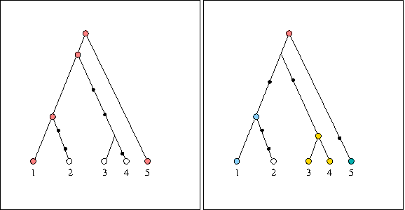
In cases where the root haplotype is not missing, as in the left-hand panel of Figure 1, we know that the ancestral location is more likely to contain that haplotype. For example, if a location contains both copies of the pink haplotype, it is more likely to be ancestral than a location which only contains younger haplotypes. If, on the other hand, the root haplotype is missing, as in the right-hand panel of Figure 1, then the ancestral location is more likely to contain immediate descendants. This approach is consistent with many descriptive characteristics of an ancestral area (Emerson and Hewitt, 2005).

OPEN IN VIEWER

FIG. 1.

Two possible genealogy scenarios, where terminal nodes represent observed sequences (with the color representing the haplotype), and small black circles are mutations. In the figure on the left, the oldest haplotype is the pink one at the top, which appears twice in the sample. In the figure on the right, the oldest haplotype is missing, and the next possible descendants are the blue, yellow, and green haplotypes.

Our heuristic approach calculates the contribution of each of the oldest observed haplotypes along all possible branches originating at the root (if the root haplotype is observed in our sample, then we simply have the root only), and then adds the contribution of each of those haplotypes for each location. For example, referring back to the right-hand panel of Figure 1, and assuming that the light blue and one of the yellow sequences appeared in location A, green in location B, and remaining yellow in location C, then the contribution of each of those haplotypes to each of the locations would be 1/4, so that the three probabilities for locations A, B, and C become 0.5, 0.25, and 0.25, respectively. If, on the other hand, the light blue sequence appeared in location A, the 2 yellow ones in location B, and green in location C, the three probabilities for locations A, B, and C become 0.33, 0.33, and 0.33, respectively. Although we do not take into account distance from the root, geographical location, or number of times each haplotype appears in a location, implicitly assuming standing variation in the population, our synthetic trials have shown that our approach provides valuable results in inferring ancestral locations.

4. Synthetic Data Analysis

We generate a set of 100 replicate synthetic datasets and assess the performance of our algorithm. Each dataset is initiated by a sequence of length l = 500, at an initial geographical location y₁₁=(0, 0) and with mutation rate \documentclass{aastex}\usepackage{amsbsy}\usepackage{amsfonts}\usepackage{amssymb}\usepackage{bm}\usepackage{mathrsfs}\usepackage{pifont}\usepackage{stmaryrd}\usepackage{textcomp}\usepackage{portland, xspace}\usepackage{amsmath, amsxtra}\pagestyle{empty}\DeclareMathSizes {10} {9} {7} {6} \begin{document} $$\frac {\theta} {2} = 1.8$$\end{document} . Each new sequence j of haplotype i then is assumed either to stay in its current location, or move to a new location: with probability 0.85 it stays in the geographical location of its ancestor a_ij such that y_ij = y_aij (implying a migration rate of 0.15); otherwise, it moves to a new location y_ij = N(y_aij, 0.1). The new sequence is forced to start a new location if the location of its ancestor contains 15 or more sequences. Extinction occurs when all of the branches of the gene tree carrying the same haplotype undergo a mutation. These tuning generative parameters were chosen in order for the synthetic datasets to match the real dataset at hand as much as possible. The iterative algorithm stops when it reaches 100 observed sequences (not including ones which are extinct in the process), corresponding to a variable number of haplotypes, locations and geographical clusters. Locations and haplotypes are ordered from oldest to most recent.

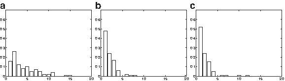
We assume both a known and an unknown tree, showing the results below. As expected, the lack of sufficient data results in weak performance at inferrring root haplotypes, as indicated by Figure 2a showing Maximum A Posteriori (MAP) estimates for the root haplotype. However, the methods are successful in inferring ancestral locations. In the case of a known haplotype tree shown in Figure 2b, the top three MAP ancestral locations cover over 90% of the cases and the corresponding percentage in the case of an unknown haplotype tree is roughly 85% (Fig. 2c). Although the data generative algorithm used here results in much stronger phylogeographic structure than observed in real datasets, it is nevetheless important to verify that our methods are able to successfully identify ancestral locations without the use of computationally expensive models.

OPEN IN VIEWER

FIG. 2.

(a) Histogram of Maximum A Posteriori (MAP) estimates for the root haplotype in the case of a known tree. (b, c) MAP estimates of ancestral locations for a known and unknown haplotype tree. Note that assessment of the ancestral haplotype inference in the case of an unknown tree is not possible, as haplotypes cannot always be uniquely identified.

We now depart from this initial set of parameters and investigate the effect of mutation and migration rates. Specifically, we set the mutation rate to θ/2 = 1.2 and θ/2 = 3 keeping all other parameters constant, with results shown in Figure 3a,b. As expected, higher mutation rates lead to higher haplotype variability and thus higher uncertainty in ancestral locations. We then fix θ/2 = 1.8 and use migration rates 0.8 and 0.9 respectively, with corresponding histograms shown in Figure 3c,d, revealing the intuitive fact that higher migration rates lead to higher ancestral location uncertainty. Note that, although the range of values for the mutation and migration rates is relatively narrow, it reflects a wide range of scenarios due to the sensitivity of the model on those parameters.

OPEN IN VIEWER

FIG. 3.

(a, b) Maximum A Posteriori histograms of the top 20 ancestral haplotypes with θ/2 = 1.2 and θ/2 = 3 respectively, migration rate 0.85. (c, d) show corresponding histograms for θ/2 = 1.8 and migration rates 0.8 and 0.9, respectively.

Finally, we use a Generalized Time-Reversible (GTR) mutation model (Tavaré, 1986) in order to address possible biases introduced by unequal mutation rates. Mutations occur as a Markov Process with generator Q-matrix \documentclass{aastex}\usepackage{amsbsy}\usepackage{amsfonts}\usepackage{amssymb}\usepackage{bm}\usepackage{mathrsfs}\usepackage{pifont}\usepackage{stmaryrd}\usepackage{textcomp}\usepackage{portland,xspace}\usepackage{amsmath,amsxtra}\pagestyle{empty}\DeclareMathSizes{10}{9}{7}{6} \begin{document} \begin{align*} Q = \phi_j \left(\begin{matrix} \cdot & v_1 \pi_G & v_2 \pi_C & v_3 \pi_T \\ v_1 \pi_A & \cdot & v_4 \pi_C & v_5 \pi_T \\ v_2 \pi_A & v_4 \pi_G & \cdot & v_6 \pi_T \\ v_3 \pi_A & v_5 \pi_G & v_6 \pi_C & \cdot\end{matrix} \right) \end{align*}\end{document}

where the π_is (i = A, G, C, T) represent the equilibrium probabilities of the nucleotides, the mutation coefficients \documentclass{aastex}\usepackage{amsbsy}\usepackage{amsfonts}\usepackage{amssymb}\usepackage{bm}\usepackage{mathrsfs}\usepackage{pifont}\usepackage{stmaryrd}\usepackage{textcomp}\usepackage{portland, xspace}\usepackage{amsmath, amsxtra}\pagestyle{empty}\DeclareMathSizes {10} {9} {7} {6} \begin{document} $$v_1, \ldots, v_6$$\end{document} the relative mutation probabilities and ϕ_j site-specific mutation coefficients. More information on the GTR mutation model can be found in Appendix C. We use the following distributions for the unknown parameters \documentclass{aastex}\usepackage{amsbsy}\usepackage{amsfonts}\usepackage{amssymb}\usepackage{bm}\usepackage{mathrsfs}\usepackage{pifont}\usepackage{stmaryrd}\usepackage{textcomp}\usepackage{portland,xspace}\usepackage{amsmath,amsxtra}\pagestyle{empty}\DeclareMathSizes{10}{9}{7}{6} \begin{document} \begin{align*} (\pi_1, \pi_2, \pi_3, \pi_4) & \sim {\cal D} (2, 2, 2, 2) \\ v_1, \ v_6 & \sim {\cal G} (1, 1) \\ v_2, \ v_3, \ v_4, \ v_5 & \sim {\cal G} (1, 7) \\ \phi_l & \sim {\cal G} (1, 0.2), \end{align*}\end{document}

so that the total migration rate θ/2 ≈ 1.8, but unevenly distributed and accounting for transition bias. Here \documentclass{aastex}\usepackage{amsbsy}\usepackage{amsfonts}\usepackage{amssymb}\usepackage{bm}\usepackage{mathrsfs}\usepackage{pifont}\usepackage{stmaryrd}\usepackage{textcomp}\usepackage{portland, xspace}\usepackage{amsmath, amsxtra}\pagestyle{empty}\DeclareMathSizes {10} {9} {7} {6} \begin{document} $${\cal G}$$\end{document} and \documentclass{aastex}\usepackage{amsbsy}\usepackage{amsfonts}\usepackage{amssymb}\usepackage{bm}\usepackage{mathrsfs}\usepackage{pifont}\usepackage{stmaryrd}\usepackage{textcomp}\usepackage{portland, xspace}\usepackage{amsmath, amsxtra}\pagestyle{empty}\DeclareMathSizes {10} {9} {7} {6} \begin{document} $${\cal D}$$\end{document} represent the Gamma and Dirichlet distributions respectively. The corresponding histogram of ancestral locations is shown in Figure 4. Despite the unequal mutation rates, results are very similar to the case of equal mutation rates. This is possibly due to the time span and size of dataset being too limited for the variable mutation rates to have a significant impact on the simulated datasets.

OPEN IN VIEWER

FIG. 4.

Histograms of Maximum A Posteriori estimates of the top 20 ancestral haplotypes using the GTR mutation model with total migration rate θ/2 = 1.8 and migration rate 0.85.

5. Real Dataset Implementation

We apply our algorithms to a mitochondrial DNA dataset of weevils in the Iberian peninsula. Rhinusa vestita is a seed parasite weevil feeding and reproducing on snapdragons. It is believed to have been present in Portugal, Spain, France, and Italy. The complete nucleotide sequence for the mitochondrial COII gene (722 bp) was obtained for 275 Rhinusa vestita individuals. Previous studies investigating the association of weevils with three host plant species, combined with knowledge about the glaciation history of the Iberian peninsula (Hewitt, 2000), led to the biological prediction that the species originated from the Rhône valley to the east and west.

We combine our methods with the analysis presented in Manolopoulou et al. (2011), in order to infer both ancestral locations but also population substructure. Manolopoulou et al. (2011) describe a model for inferring phylogeographic substructure by identifying population clusters consistent with individual migrations, but without providing temporal results such as ancestral locations. Here, we combine these methods with our ancestral inference within the same Markov chain Monte Carlo inference, in order to provide results both on population substructure as well as geographical origin.

The results confirm the biological hypothesis of the location of origin; the top four sampling locations, collecting 75% of posterior mass, are shown in Table 1. As in Manolopoulou et al. (2011), we plot what is now a rooted gene tree shown in Figure 5, using color to indicate geographical population cluster (in contrast to Fig. 1, where color represented haplotype). Here, each color represents a geographically relatively homogeneous population, and each new cluster (and corresponding color) is formed via migration. Figure 6 shows the corresponding geographical distribution of each of the population clusters, with the larger spot representing the most likely ancestral location. Combined with our ancestral location inference methods, it appears that weevils originated around the Rhône valley, migrating to the east and west, in agreement with biological predictions.

OPEN IN VIEWER

FIG. 5.

One of the non-unique MAP estimates of the haplotype tree using our approach, where color corresponds to cluster and size to the number of individuals sampled with each sequence.

OPEN IN VIEWER

FIG. 6.

Corresponding bivariate normal contour plots evaluated at the posterior means for the weevil dataset. The black dots indicate sampling locations, and colors correspond to the clusters shown in Figure 5. The largest dot corresponds to the MAP ancestral location.

6. Discussion

We have presented a statistical framework whereby the coalescent model is used in order to draw inferences about haplotype trees through Markov chain Monte Carlo. In addition, we have described methods for inferring ancestral locations in phylogeographic settings. Our results were validated by simulated synthetic datasets, and were successful in confirming the biological hypothesis in the real dataset.

Although more sophisticated evolutionary models may be used to account for a variable population size (Slatkin, 2001), selection (Neuhauser and Krone, 1997), and recombination (Hudson and Kaplan, 1988), prior implementations we ran showed that in small-scale datasets such as the one at hand, the data are very weakly informative about many of the additional evolutionary parameters. Perhaps the most valuable extension would allow for the coalescence rate to vary across population clusters, in order to represent local proliferations. Similarly, rigorous theoretical calculations relating ancestral haplotypes with geographical locations (Bloomquist et al., 2010; Lemey et al., 2010, 2009), perhaps through the use of an explicit migration model, can provide a solid basis for an improved estimator of ancestral locations.

Finally, our methods are freely available through an R package “Bayesian Phylogeographic Clustering” (available at www.stat.duke.edu/∼im30/software.html).

Appendix

A. Haplotype tree example

Suppose the haplotype tree is given by the top tree of Figure 7. For ease of exposition, the numbers on the nodes here represent the sample sizes of each haplotype rather than the label of each haplotype, and we represent each event by updating the numbers on each haplotype according to the number of times it is observed at each time-point in the sample.

OPEN IN VIEWER

FIG. 7.

(Top) In this tree the MRCA of the sample (top) is observed twice in the sample. Note that one of the intermediate haplotypes is not observed in the sample (and hence has zero sample size). (Bottom) A possible scenario for how the present sample came about. Nodes without a number represent haplotypes that have not arisen yet. At first one sequence is present, the ancestral sequence, which split into two (remember that the first event is always a split). Then one of those two identical sequences split again to give us a total of three. One of those three then mutates to give rise to the intermediate haplotype, which in turn splits and then mutates (and goes extinct) to give us the right-hand leaf. Finally, the intermediate haplotype mutates again to give us the left-hand leaf, which subsequently splits to give another copy of itself.

Simulating a temporal ordering implies that, starting with the ancestral sequence, we specify a series of split and mutation events which occurred by mimicking evolution, eventually resulting in the fixed haplotype tree. For example, the bottom panel of Figure 7 is a possible temporal ordering of the observed tree given in the top panel.

Observe now that, for example, the root node could not have split any further: this would result in three copies of the ancestral haplotype, which is inconsistent with the haplotype tree which specifies precisely two. In addition, it would not have been possible for the intermediate haplotype to mutate after Step 3 above, since then it would disappear from the ancestral sequences, and another mutation would not have been possible. In other words, consistent events are defined as follows.

• A split event is consistent with the haplotype tree, if it does not imply that the sample size of that haplotype will exceed the number of times it appears in the complete haplotype tree, plus the number of mutations that haplotype will be forced to undergo in following steps (so, in the example, the intermediate haplotype after Step 5 will be forced to undergo exactly one more mutation).

• Similarly, a mutation is possible if (a) is true, and (b) OR (c) are true:

(a) it is represented by an edge on the haplotype tree, where the ancestral sequence of the edge has already appeared in the ancestral sample;

(b) the ancestral sequence of the edge corresponding to that mutation does not go extinct;

(c) the ancestral sequence of the edge goes extinct, and there are not more events involving that sequence which have not yet occurred but are forced by the haplotype tree.

Disclosure Statement

No competing financial interests exist.