Finding Maximum Colorful Subtrees in Practice

Abstract

In metabolomics and other fields dealing with small compounds, mass spectrometry is applied as a sensitive high-throughput technique. Recently, fragmentation trees have been proposed to automatically analyze the fragmentation mass spectra recorded by such instruments. Computationally, this leads to the problem of finding a maximum weight subtree in an edge-weighted and vertex-colored graph, such that every color appears, at most once in the solution. We introduce new heuristics and an exact algorithm for this Maximum Colorful Subtree problem and evaluate them against existing algorithms on real-world and artificial datasets. Our tree completion heuristic consistently scores better than other heuristics, while the integer programming-based algorithm produces optimal trees with modest running times. Our fast and accurate heuristic can help determine molecular formulas based on fragmentation trees. On the other hand, optimal trees from the integer linear program are useful if structure is relevant, for example for tree alignments.

1. Introduction

Mass spectrometry is one of the prevalent technologies for the analysis of metabolites and other small compounds with mass below 1000 Da. The study of such compounds is, for example, relevant in drug design and the search for new signaling molecules and biomarkers (Li and Vederas, 2009). Typically, the analyte is fragmented in the mass spectrometer such that fragment masses and their intensities can be recorded in a fragmentation spectrum. Usually, this spectrum is then compared to a database of reference spectra (Oberacher et al., 2009). Unfortunately, such databases are vastly incomplete (Fernie et al., 2004). Thus, de novo approaches, which try to identify the compound based solely on its spectrum, are sought. Whereas de novo interpretation of protein spectra makes use of their specific structure, this is not possible for metabolites, as they are not structurally restricted.

Böcker and Rasche (2008) suggested fragmentation trees for the de novo interpretation of metabolite tandem mass spectrometry data. Fragmentation trees can be used to identify the molecular formula of a compound (Böcker and Rasche, 2008), as well as to describe the fragmentation process (Rasche et al., 2011). Fragmentation trees can also be used for the interpretation of gas chromatography (GC) mass spectrometry, where fragmentation is induced by electron ionization (EI) (Hufsky et al., 2012b), as well as multiple mass spectrometry (MSⁿ) (Scheubert et al., 2011). The automated alignment of such fragmentation trees (Hufsky, et al., 2012a; Rasche et al., 2012) seems to be a particularly promising approach, allowing a fully automated computational identification of small molecules that cannot be found in any database, and paving the way toward natural product discovery, searching for signaling molecules, biomarkers, novel or illegal drugs, or other “interesting” organic compounds.

It must be understood that, depending on the application at hand, different aspects of fragmentation tree computation are most relevant: In case we want to identify the molecular formula of an unknown (Böcker and Rasche, 2008; Hufsky, 2012b) then swift computations are mandatory, as we might have to compute hundreds of trees for a single compound. But if we want to (manually or automatically) interpret the structure of fragmentation trees (Rasche et al., 2011, 2012), then it is presumably beneficial to use optimal solutions. Calculating fragmentation trees leads to the Maximum Colorful Subtree problem (Böcker and Rasche, 2008).

Maximum Colorful Subtree Problem. Given a vertex-colored DAG G = (V, E) with colors and weights w : E → \documentclass{aastex}\usepackage{amsbsy}\usepackage{amsfonts}\usepackage{amssymb}\usepackage{bm}\usepackage{mathrsfs}\usepackage{pifont}\usepackage{stmaryrd}\usepackage{textcomp}\usepackage{portland, xspace}\usepackage{amsmath, amsxtra}\pagestyle{empty}\DeclareMathSizes{10}{9}{7}{6}\begin{document} $${\mathbb R}$$ \end{document} , find the induced colorful subtree T = (V_T, E_T) of G of maximum weight \documentclass{aastex}\usepackage{amsbsy}\usepackage{amsfonts}\usepackage{amssymb}\usepackage{bm}\usepackage{mathrsfs}\usepackage{pifont}\usepackage{stmaryrd}\usepackage{textcomp}\usepackage{portland, xspace}\usepackage{amsmath, amsxtra}\pagestyle{empty}\DeclareMathSizes{10}{9}{7}{6}\begin{document} $$w (T) : = \sum \nolimits_{e \in E_T}w (e)$$ \end{document} .

This is a special case of the edge-weighted Graph Motif problem (see Sikora, 2010, for an overview). Scheubert et al. (2011) present the related Colorful Subtree Closure problem for analyzing multiple mass spectrometry data. Ljubić et al. (2005) presented an integer linear program for the related Prize-Collecting Steiner Tree problem. The Maximum Colorful Subtree problem is NP-hard (Fellows et al., 2006) as well as APX-hard (Dondi et al., 2009) even on binary trees. Furthermore, on general trees it has no constant factor approximation (Dondi et al., 2009; Sikora, 2011).

This article presents an experimental study of various heuristics for the Maximum Colorful Subtree problem. We implement a new heuristic along with naive greedy approaches and three exact algorithms for the problem. The various algorithms are then compared with respect to their running times and quality of the generated trees. As a side result, we prove that even after relaxing the color constraints, the resulting Maximum Subtree problem remains inapproximable within O(|V|^1−ε) factor for any ε > 0, unless P = NP. Our proof is simpler and improves upon the previous APX-hardness result due to Dondi et al. (2009) under the same complexity hypothesis. Sikora (2011) showed a slightly weaker inapproximability result for unweighted graphs but maintained the color constraints.

The rest of the article is organized as follows: The next section defines the Maximum Colorful Subtree problem and describes how it is applied to analyze tandem mass spectra. In Section 3, we discuss the computational complexity of the closely related Maximum Subtree problem. Exact and heuristic algorithms for the Maximum Colorful Subtree problem are presented in Section 4. In Section 5, we evaluate these algorithms on three real-world and two artificial datasets.

2. Computing Fragmentation Trees

Here we outline our method of computing the fragmentation tree of a metabolite compound from its tandem mass spectrum. This leads to a formal definition of the Maximum Colorful Subtree problem. Let \documentclass{aastex}\usepackage{amsbsy}\usepackage{amsfonts}\usepackage{amssymb}\usepackage{bm}\usepackage{mathrsfs}\usepackage{pifont}\usepackage{stmaryrd}\usepackage{textcomp}\usepackage{portland, xspace}\usepackage{amsmath, amsxtra}\pagestyle{empty}\DeclareMathSizes{10}{9}{7}{6}\begin{document} $$m_1 , \ldots , m_p$$ \end{document} be the peak masses of a spectrum consisting of p peaks. We first compute a list of possible molecular formulas \documentclass{aastex}\usepackage{amsbsy}\usepackage{amsfonts}\usepackage{amssymb}\usepackage{bm}\usepackage{mathrsfs}\usepackage{pifont}\usepackage{stmaryrd}\usepackage{textcomp}\usepackage{portland, xspace}\usepackage{amsmath, amsxtra}\pagestyle{empty}\DeclareMathSizes{10}{9}{7}{6}\begin{document} $$\{F_i^1 , \ldots , F_i^{n_i} \} $$ \end{document} with mass close to m_i for each 1 ≤ i ≤ p. We then construct a directed acyclic graph G, where the set of vertices are the molecular formulas \documentclass{aastex}\usepackage{amsbsy}\usepackage{amsfonts}\usepackage{amssymb}\usepackage{bm}\usepackage{mathrsfs}\usepackage{pifont}\usepackage{stmaryrd}\usepackage{textcomp}\usepackage{portland, xspace}\usepackage{amsmath, amsxtra}\pagestyle{empty}\DeclareMathSizes{10}{9}{7}{6}\begin{document} $$F_i^j$$ \end{document} of the i-th peak, for 1 ≤ j ≤ n_i and 1 ≤ i ≤ p. Next, we label the vertices with colors from \documentclass{aastex}\usepackage{amsbsy}\usepackage{amsfonts}\usepackage{amssymb}\usepackage{bm}\usepackage{mathrsfs}\usepackage{pifont}\usepackage{stmaryrd}\usepackage{textcomp}\usepackage{portland, xspace}\usepackage{amsmath, amsxtra}\pagestyle{empty}\DeclareMathSizes{10}{9}{7}{6}\begin{document} $$\{1 , \ldots , p \} $$ \end{document} , where all vertices corresponding to the i-th peak are assigned color i. We connect two vertices u, v with a directed edge uv, if the molecular formula of v is a sub-formula of the formula of u, that is, v contains at most as many atoms of every chemical element as u. The edge uv thus represents a possible fragmentation step of the molecule associated with u, (see Fig. 1 for an example). Note that G is acyclic, since the subset relation used to define edges is a partial order.

FIG. 1.

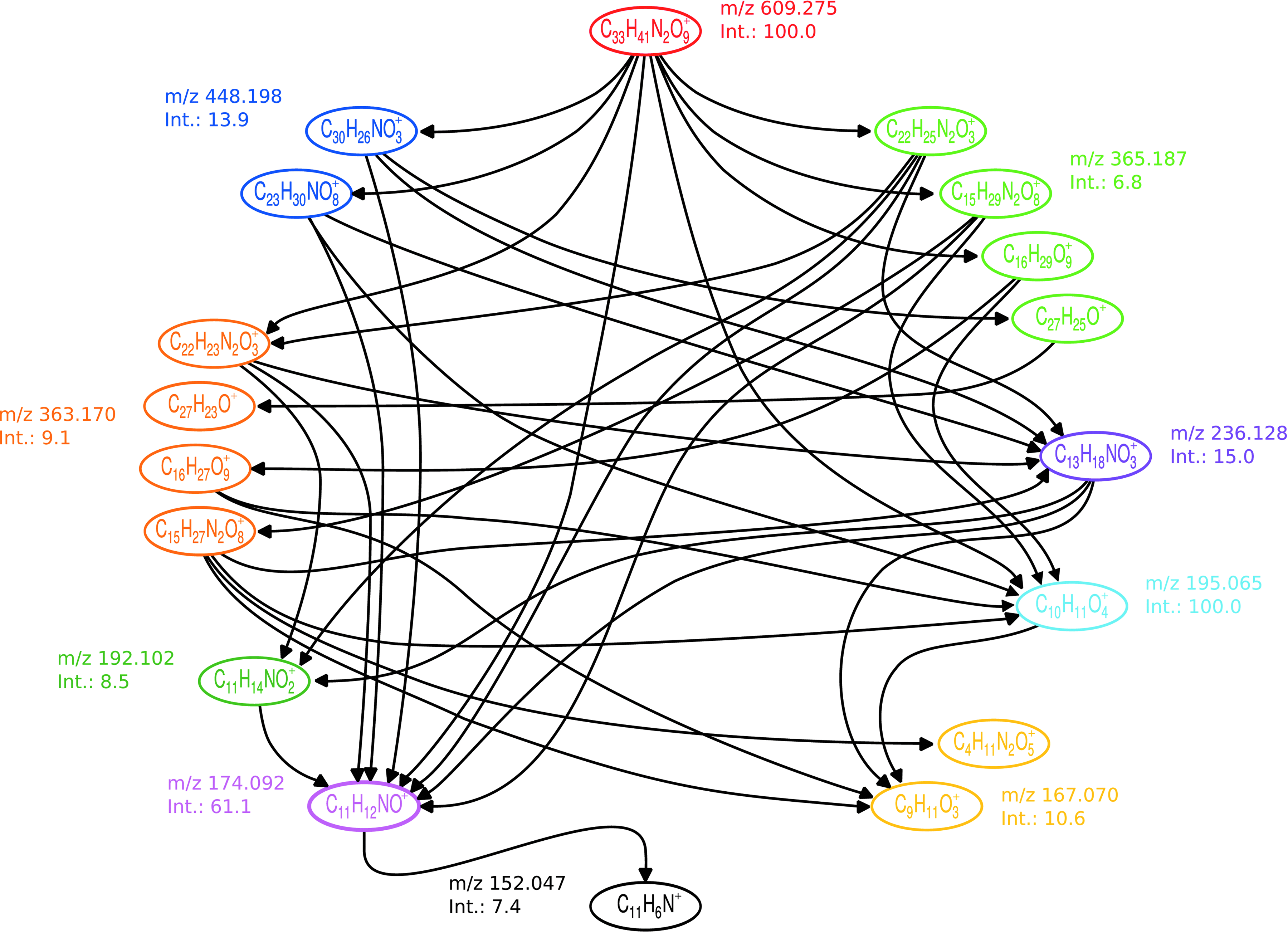
Input graph calculated from the spectrum of Reserpine (micromass dataset). Formulas of identically colored nodes have nearly identical masses. Edges are drawn between vertices if the molecular formula of one vertex is a subformula of the molecular formula of the other.

Let us assume that the largest peak mass is m₁, which corresponds to the unfragmented compound whose fragmentation tree we want to compute. We further assume without loss of generality that n₁ = 1, otherwise we can consider a separate graph for each molecular formula explaining the peak mass m₁. So, we may assume that there is only a single source vertex r associated with the unfragmented compound. We delete all other vertices without incoming edges from the graph, since they cannot be part of the fragmentation process. Consequently, G is a directed acyclic graph (DAG) with unique source r such that every other node is reachable from r.

A subtree of G is colorful if any two vertices in the tree have different colors. A colorful subtree of G rooted at r explains each peak in the input mass spectrum at most once. The approach of Rasche et al. (2011) works by scoring edges by log likelihoods of the fragmentation steps to which they correspond. Thus, edges may have negative weights. The maximum colorful subtree rooted at r will then be the most likely explanation of the given mass spectrum.

3. Complexity Results for the Maximum Subtree Problem

We now consider a relaxation of the maximum colorful subtree problem obtained by dropping the color constraints. The resulting Maximum Subtree problem asks to find a maximum weight tree rooted at a particular vertex in the given edge-weighted DAG G = (V, E). It turns out that this simpler problem is still NP-hard. In fact, this problem is NP-hard to approximate within O(|V|^1−ε) factor for any ε > 0.

Theorem 1. There is no O(|V|^1−ε) approximation algorithm for the Maximum Subtree problem for any ε > 0, unless P = NP.

Proof. The reduction is from the maximum independent set problem, which, for a given graph G′ = (V, E) and a positive integer k, asks to decide if there is a subset of vertices in V of size at least k such that it contains no edge from E. Let \documentclass{aastex}\usepackage{amsbsy}\usepackage{amsfonts}\usepackage{amssymb}\usepackage{bm}\usepackage{mathrsfs}\usepackage{pifont}\usepackage{stmaryrd}\usepackage{textcomp}\usepackage{portland, xspace}\usepackage{amsmath, amsxtra}\pagestyle{empty}\DeclareMathSizes{10}{9}{7}{6}\begin{document} $$V = \{v_1 , \ldots , v_n \} $$ \end{document} and \documentclass{aastex}\usepackage{amsbsy}\usepackage{amsfonts}\usepackage{amssymb}\usepackage{bm}\usepackage{mathrsfs}\usepackage{pifont}\usepackage{stmaryrd}\usepackage{textcomp}\usepackage{portland, xspace}\usepackage{amsmath, amsxtra}\pagestyle{empty}\DeclareMathSizes{10}{9}{7}{6}\begin{document} $$E = \{E_1 , \ldots , E_m \} $$ \end{document} where n = |V| and m = |E|. We construct a DAG G with four layers of vertices: The first layer consists of a single source s. The second layer consists of single vertex u connected with source s with an edge weighted −n(m − 1). The third layer consists of n vertices \documentclass{aastex}\usepackage{amsbsy}\usepackage{amsfonts}\usepackage{amssymb}\usepackage{bm}\usepackage{mathrsfs}\usepackage{pifont}\usepackage{stmaryrd}\usepackage{textcomp}\usepackage{portland, xspace}\usepackage{amsmath, amsxtra}\pagestyle{empty}\DeclareMathSizes{10}{9}{7}{6}\begin{document} $$x_1 , \ldots , x_n$$ \end{document} , each of which has an incoming edge from u with weight −1. The fourth layer consists of m vertices \documentclass{aastex}\usepackage{amsbsy}\usepackage{amsfonts}\usepackage{amssymb}\usepackage{bm}\usepackage{mathrsfs}\usepackage{pifont}\usepackage{stmaryrd}\usepackage{textcomp}\usepackage{portland, xspace}\usepackage{amsmath, amsxtra}\pagestyle{empty}\DeclareMathSizes{10}{9}{7}{6}\begin{document} $$y_1 , \ldots , y_m$$ \end{document} . The vertex y_i has an incoming edge from the vertex x_j with weight n whenever \documentclass{aastex}\usepackage{amsbsy}\usepackage{amsfonts}\usepackage{amssymb}\usepackage{bm}\usepackage{mathrsfs}\usepackage{pifont}\usepackage{stmaryrd}\usepackage{textcomp}\usepackage{portland, xspace}\usepackage{amsmath, amsxtra}\pagestyle{empty}\DeclareMathSizes{10}{9}{7}{6}\begin{document} $$v_j \in E_i$$ \end{document} (Fig. 2).

FIG. 2.

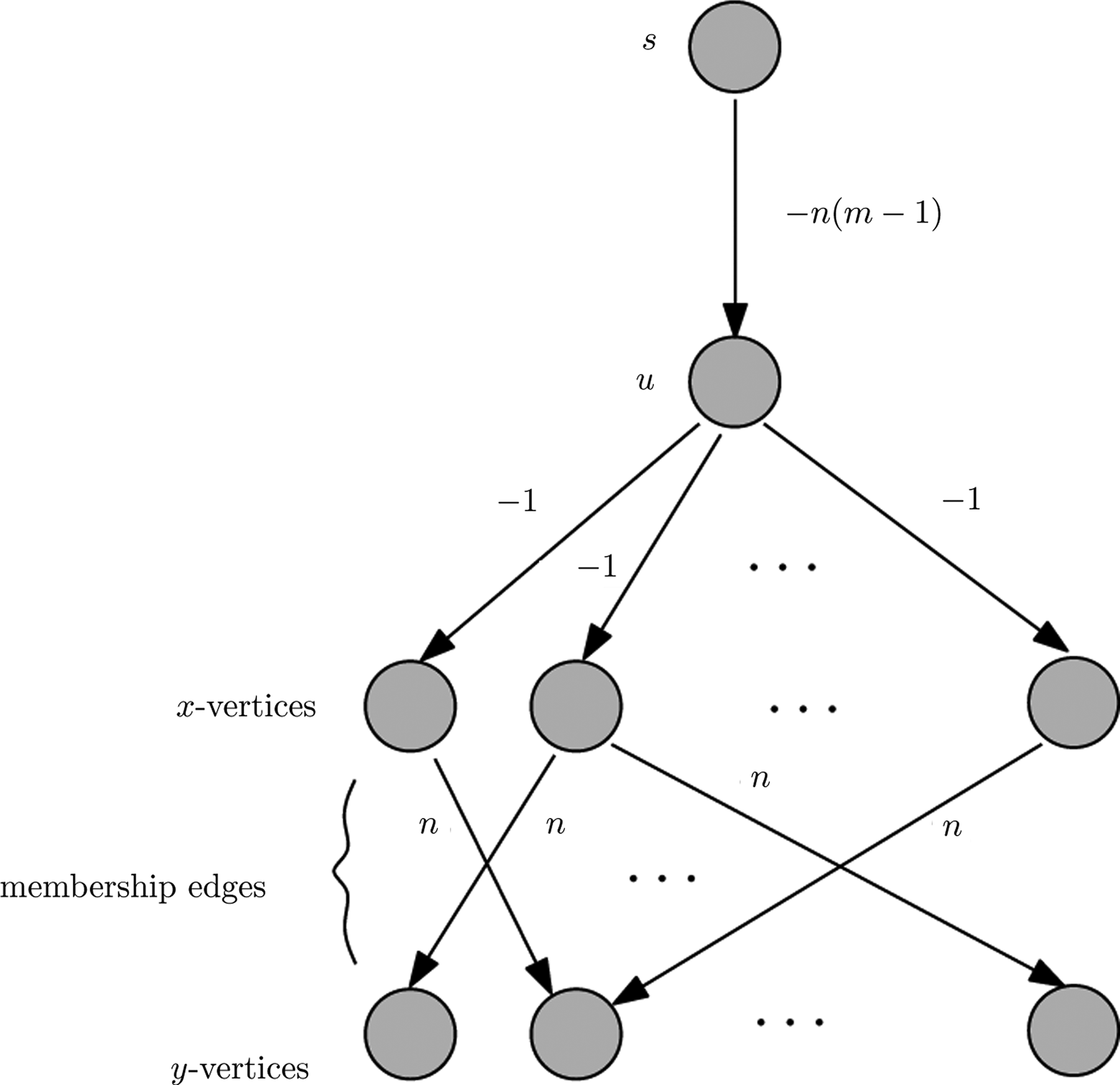
Proof of Theorem 1.

Given an independent set I ⊆ V of size k = |I| in G′, we construct a tree T of weight k as follows. The vertex set of T consists of vertices s, u, all of the y-vertices, and the subset from x-vertices of size k′ = n − k such that their corresponding vertex in G′ is not in I. Note that since I is an independent set in G′, the selected subset of x-vertices is connected with all y-vertices. The edge set of T consists of the edge (s, u), the k′ edges from u to the selected subset of x-vertices, and m edges from x-vertices to y-vertices such that each y-vertex has exactly one incoming edge. Clearly T is a connected tree and has total weight −n(m − 1) − k′ + mn = n − k′ = k.

Conversely, let T be an s-rooted subtree of G of weight k = n − k′ such that there is no other subtree of larger weight in G. Then it is easy to see that it necessarily contains all y-vertices from G since otherwise we can increase the weight of T by n by adding a y-vertex that was not present before in T (we may need to add an x-vertex to be able to connect to that y-vertex but this only incurs −1 cost). Also note that T must contain the edge (s, u) so that T is connected with the root s. Let us assume that T contains k′ x-vertices and let H be the corresponding set of vertices in G′. It follows that V\H is a maximum independent set in G′ since otherwise we again can increase the cost of T by choosing a smaller number of x-vertices in T. So the maximum independent set in G′ has to be of size n − k′ = k. ▪

Note that the inapproximability result from Theorem 1 also holds for the Maximum Colorful Subtree problem, since it is a generalization of the Maximum Subtree problem.

4. Algorithms for the Maximum Colorful Subtree Problem

In this section, we briefly review exact algorithms as well as heuristics for the Maximum Colorful Subtree problem. We conclude the section with two new heuristics for the problem.

For vertices u and v, let c(v) be the color assigned to v and \documentclass{aastex}\usepackage{amsbsy}\usepackage{amsfonts}\usepackage{amssymb}\usepackage{bm}\usepackage{mathrsfs}\usepackage{pifont}\usepackage{stmaryrd}\usepackage{textcomp}\usepackage{portland, xspace}\usepackage{amsmath, amsxtra}\pagestyle{empty}\DeclareMathSizes{10}{9}{7}{6}\begin{document} $$w (u , v) \in {\mathbb R}$$ \end{document} the weight of the edge uv. Throughout the rest of the article we denote the number of colors in G = (V, E) by k. Note that k ≤ p can be as large as the number of peaks in the spectrum, but we can also choose a smaller k to decrease running times, limiting our attention to, say, the k most intense peaks.

4.1. Exact methods

The problem can be solved exactly by using dynamic programming over vertices and color subsets (Dreyfus and Wagner, 1972). Let W(v, S) be the maximal score of a colorful tree with root v and color set S ⊆ C. Now, table W can be computed by the following recurrence (Böcker and Rasche, 2008): \documentclass{aastex}\usepackage{amsbsy}\usepackage{amsfonts}\usepackage{amssymb}\usepackage{bm}\usepackage{mathrsfs}\usepackage{pifont}\usepackage{stmaryrd}\usepackage{textcomp}\usepackage{portland, xspace}\usepackage{amsmath, amsxtra}\pagestyle{empty}\DeclareMathSizes{10}{9}{7}{6}\begin{document} \begin{align*}\openup5ptW (v , S) = \max \begin{cases} \max \limits_{u:c (u) \in S \setminus \{c (v) \} , vu \in E} W (u , S \setminus \{c (v) \}) + w (v , u) \\ \max \limits_{(S_1 , S_2) : S_1 \cap S_2 = \{c (v) \} , S_1 \cup S_2 = S} W (v , S_1) + W (v , S_2) \end{cases}\end{align*} \end{document}

where, obviously, we have to exclude the cases S₁ = {c(v)} and S₂ = {c(v)} from the computation of the second maximum. Using the above recurrence with the initial condition W(v,{c(v)}) = 0, we can compute a maximum colorful tree in O(3^kk|E|) time and O(2^k|V|) space. The exponential running time and space make the algorithm useful only for small size instances. The running time can be somewhat improved to O(2^k · poly(|V|, k)) by using the Möbius transform and the inversion technique of Björklund et al. (2007). However, the technique only works for suitably small integer weights.

Guillemot and Sikora (2010) suggest a different approach using multilinear detection (Koutis and Williams, 2009) for input graphs with unit weights. Their algorithm requires O(2^k · poly(|E|, k)) time and only polynomial space. The algorithm can be adopted to integer weight graphs in a straightforward manner but the resulting algorithm would be pseudo-polynomial; that is, its running time would depend polynomially on the integer weights, thus making it impractical for our purposes. To the best of our knowledge, neither the above algorithm nor the dynamic programming with Möbius transform have been used in implementations.

For small instances, a brute-force approach is suggested by Böcker and Rasche (2008). The idea is to find a maximum subtree for each possible combination of vertices forming a colorful set. We then search a maximum subtree in a colorful DAG. Clearly, when all edge weights are positive, then the maximum subtree is a spanning tree. This can be found by a simple greedy algorithm, choosing the maximum weight incoming edge for each vertex but the root. With arbitrary edge weights, the problem becomes NP-hard, as shown in Section 3. We solve the problem naively by iterating over all combinations of vertices whose best incoming edge has a negative weight. The brute-force approach is obviously not practical when either the number of combinations is large or when there are many vertices whose maximum incoming edge has negative weight.

Integer Linear Programming. Let us define a binary variable x_uv for each edge uv of the input graph. For each color \documentclass{aastex}\usepackage{amsbsy}\usepackage{amsfonts}\usepackage{amssymb}\usepackage{bm}\usepackage{mathrsfs}\usepackage{pifont}\usepackage{stmaryrd}\usepackage{textcomp}\usepackage{portland, xspace}\usepackage{amsmath, amsxtra}\pagestyle{empty}\DeclareMathSizes{10}{9}{7}{6}\begin{document} $$c \in C$$ \end{document} let V (c) be the set of all vertices in G = (V, E), which are colored with c. Then the following simple integer linear program (ILP) captures the maximum colorful subtree problem: \documentclass{aastex}\usepackage{amsbsy}\usepackage{amsfonts}\usepackage{amssymb}\usepackage{bm}\usepackage{mathrsfs}\usepackage{pifont}\usepackage{stmaryrd}\usepackage{textcomp}\usepackage{portland, xspace}\usepackage{amsmath, amsxtra}\pagestyle{empty}\DeclareMathSizes{10}{9}{7}{6}\begin{document} \begin{align*} \max \sum_{uv \in E} w(u, v) \cdot x_{uv} \tag{1}\end{align*} \end{document} \documentclass{aastex}\usepackage{amsbsy}\usepackage{amsfonts}\usepackage{amssymb}\usepackage{bm}\usepackage{mathrsfs}\usepackage{pifont}\usepackage{stmaryrd}\usepackage{textcomp}\usepackage{portland, xspace}\usepackage{amsmath, amsxtra}\pagestyle{empty}\DeclareMathSizes{10}{9}{7}{6}\begin{document} \begin{align*} {\rm s.t.} \sum_{u \ {\rm with} \ uv \in E} x_{uv} \leq 1 \qquad \qquad \qquad \qquad \qquad \qquad \qquad {\rm for \ all} \ v \in V \setminus \{r \} , \tag{2}\end{align*} \end{document} \documentclass{aastex}\usepackage{amsbsy}\usepackage{amsfonts}\usepackage{amssymb}\usepackage{bm}\usepackage{mathrsfs}\usepackage{pifont}\usepackage{stmaryrd}\usepackage{textcomp}\usepackage{portland, xspace}\usepackage{amsmath, amsxtra}\pagestyle{empty}\DeclareMathSizes{10}{9}{7}{6}\begin{document} \begin{align*}x_{vw} \leq \sum_{u \ {\rm with} \ uv \in E} x_{uv} \qquad {\rm for \ all} \ vw \in E \ {\rm with} \ v \neq r , \tag{3}\end{align*} \end{document} \documentclass{aastex}\usepackage{amsbsy}\usepackage{amsfonts}\usepackage{amssymb}\usepackage{bm}\usepackage{mathrsfs}\usepackage{pifont}\usepackage{stmaryrd}\usepackage{textcomp}\usepackage{portland, xspace}\usepackage{amsmath, amsxtra}\pagestyle{empty}\DeclareMathSizes{10}{9}{7}{6}\begin{document} \begin{align*} \sum_{uv \in E \ {\rm with} \ v \in V (c)} x_{uv} \leq 1 \qquad \qquad \qquad \qquad \qquad \qquad \qquad {\rm for \ all} \ c \in C , \tag{4}\end{align*} \end{document} \documentclass{aastex}\usepackage{amsbsy}\usepackage{amsfonts}\usepackage{amssymb}\usepackage{bm}\usepackage{mathrsfs}\usepackage{pifont}\usepackage{stmaryrd}\usepackage{textcomp}\usepackage{portland, xspace}\usepackage{amsmath, amsxtra}\pagestyle{empty}\DeclareMathSizes{10}{9}{7}{6}\begin{document} \begin{align*} x_{uv} \in \{0 , 1 \} \qquad \qquad \qquad \qquad \qquad \qquad {\rm for \ all} \ uv \in E. \tag{5} \end{align*} \end{document}

In the above integer program, the constraints set Equation (2) ensures that the feasible solution is a forest, whereas the constraints set Equation (4) makes sure that there is at most one vertex of each color present in the solution. Finally, Equation (3) requires the solution to be connected. Note that in general graphs, we would have to ensure for every cut of the graph to be connected to some parent vertex. That would require an exponential number of constraints (Ljubić et al., 2005). But since our graph is directed and acyclic, a linear number of constraints suffice.

4.2. Heuristics

A simple greedy heuristic has been proposed in Böcker and Rasche (2008). It works by considering the edges according to their weights in descending order. The edge being considered is added to the result, if it does not conflict with the previously picked edges. The algorithm continues until all positive edges are considered and the resulting graph is connected. Note that an edge conflicts with another if they are either incoming edges to the same vertex or are incident edges to different vertices of the same color. Finally, we prune the leaves that are attached by negative weight edges in the resulting spanning tree. We refer to the above heuristic as greedy in the rest of the article.

Another greedy strategy is to consider colors in some ordering and add a vertex of the current color that promises the maximum increase of the score and attaches it to the already calculated tree. The resulting heuristic, referred to as the insertion heuristic, begins with only the root as the current partial solution. The heuristic greedily attaches vertices labeled with unused colors. For every vertex u with unused color, and every vertex v already part of the solution, we calculate how much we gain by attaching u to v. To calculate the gain of attaching u to v, we take into account the score of the edge vu, as well as the possibility of rerouting other outgoing edges of v through u. The vertex with maximum gain is then attached to the solution and edges are rerouted as required. (See Algorithm 1 for details.) In our implementation, we choose the colors in Line 2 of the algorithm in descending order with respect to the intensities of their corresponding peaks in the real-world datasets.

Algorithm 1: Vertex insertion heuristic
Input: An edge-weighted and vertex-colored DAG G, \documentclass{aastex}\usepackage{amsbsy}\usepackage{amsfonts}\usepackage{amssymb}\usepackage{bm}\usepackage{mathrsfs}\usepackage{pifont}\usepackage{stmaryrd}\usepackage{textcomp}\usepackage{portland, xspace}\usepackage{amsmath, amsxtra}\pagestyle{empty}\DeclareMathSizes{10}{9}{7}{6}\begin{document} $$r \in V (G)$$ \end{document} , and color set C.
Output: A colorful subtree rooted at r.
1:	T := {r}.
2:	for all \documentclass{aastex}\usepackage{amsbsy}\usepackage{amsfonts}\usepackage{amssymb}\usepackage{bm}\usepackage{mathrsfs}\usepackage{pifont}\usepackage{stmaryrd}\usepackage{textcomp}\usepackage{portland, xspace}\usepackage{amsmath, amsxtra}\pagestyle{empty}\DeclareMathSizes{10}{9}{7}{6}\begin{document} $$c \in C$$ \end{document} such that c does not appear in T do
3:	Let v be a c-colored vertex that maximizes the quantity
	\documentclass{aastex}\usepackage{amsbsy}\usepackage{amsfonts}\usepackage{amssymb}\usepackage{bm}\usepackage{mathrsfs}\usepackage{pifont}\usepackage{stmaryrd}\usepackage{textcomp}\usepackage{portland, xspace}\usepackage{amsmath, amsxtra}\pagestyle{empty}\DeclareMathSizes{10}{9}{7}{6}\begin{document} $$w (u , v) + \displaystyle\sum_{w (v , x) > w (u , x)} (w (v , x) - w (u , x)) ,$$ \end{document}
	where u, x are vertices in T.
4:	Add uv to T.
5:	Add vx and remove ux for all \documentclass{aastex}\usepackage{amsbsy}\usepackage{amsfonts}\usepackage{amssymb}\usepackage{bm}\usepackage{mathrsfs}\usepackage{pifont}\usepackage{stmaryrd}\usepackage{textcomp}\usepackage{portland, xspace}\usepackage{amsmath, amsxtra}\pagestyle{empty}\DeclareMathSizes{10}{9}{7}{6}\begin{document} $$x \in T$$ \end{document} for which w(v, x) > w(u, x) holds.
6:	return T.

Tree Completion Heuristic. As noted before, the dynamic programming (DP) approach of Section 4.1 works only for small inputs. We now present a heuristic that combines DP with the greedy approaches. For a small enough constant b, the heuristic works by first computing the maximum colorful subtree consisting of at most b vertices, which we call backbone of a candidate solution. Next, we complete the backbone by using one of the greedy heuristics discussed above.

The tree completion heuristic works with Algorithm 1 by initializing T in Line 1 with the computed backbone. Similarly, the greedy heuristic can be used to complete the tree by starting with the backbone and applying the greedy heuristic on the remaining edges. In our experiments, we use the insertion heuristic for tree completion since it achieved consistently better scores. This heuristic is referred to as DP_b, where b is the size of the backbone computed exactly.

5. Evaluation Results

In our study, we analyze spectra from three real and two randomly generated datasets. The Orbitrap dataset consists of mass spectra of 38 compounds with a mass accuracy of 10 ppm. It includes the 37 compounds used for evaluating fragmentation trees in Rasche et al. (2011). The Micromass dataset (Hill et al., 2008) contains spectra of 100 compounds with an accuracy of 50 ppm, while the QSTAR dataset (Böcker and Rasche, 2008) consists of 36 mass spectra with 20 ppm accuracy. Note that the later dataset contains only 14.3 peaks per compound on average, whereas the average for Orbitrap and Micromass datasets is 75.4 and 51.6 peaks per compound, respectively. The Orbitrap dataset contains 1.03 vertices per color, the Hill dataset 1.7, and the QSTAR dataset has 1.1 vertices per color. Despite these low ratios, the number of colorful vertex sets grows as large as 10⁵⁵ for certain instances due to the combinatorial explosion. Experimental details can be found in the corresponding publications.

For each compound in the above three datasets, we assume that we know the correct molecular formula and construct a directed acyclic graph as described in Section 2. We use the scoring from Rasche et al. (2011) to weight the edges.

Our first randomly generated dataset, called Random, consists of 17 DAGs with the number of colors ranging from 20 to 100 in steps of five. We generate three vertices for every color except the root, which is a unique vertex with color 0. For k colors, our DAG consists of 3(k − 1) + 1 vertices and \documentclass{aastex}\usepackage{amsbsy}\usepackage{amsfonts}\usepackage{amssymb}\usepackage{bm}\usepackage{mathrsfs}\usepackage{pifont}\usepackage{stmaryrd}\usepackage{textcomp}\usepackage{portland, xspace}\usepackage{amsmath, amsxtra}\pagestyle{empty}\DeclareMathSizes{10}{9}{7}{6}\begin{document} $$ \frac {9} {2} k (k - 1) - 6 (k - 1)$$ \end{document} edges, where each vertex with color i is connected to all vertices colored \documentclass{aastex}\usepackage{amsbsy}\usepackage{amsfonts}\usepackage{amssymb}\usepackage{bm}\usepackage{mathrsfs}\usepackage{pifont}\usepackage{stmaryrd}\usepackage{textcomp}\usepackage{portland, xspace}\usepackage{amsmath, amsxtra}\pagestyle{empty}\DeclareMathSizes{10}{9}{7}{6}\begin{document} $$i + 1 , \ldots , k$$ \end{document} and has weight drawn from normal distribution with mean −8 and standard deviation 10. And finally the last dataset we consider is called Hard, which is generated with Model RB of Xu and Li (2006). It produces instances of constraint satisfaction problem (CSP) with exponential resolution proof complexity (with high probability). For each 10 < c ≤ 30, we generate a CSP instance with constraint sizes c and convert these CSP instances to the instances of Maximum Subtree problem using a standard reduction to the maximum independent set problem and the reduction of Section 3.

We implemented the exact algorithms based on the dynamic program, the integer linear program, and the brute-force approach of Section 4.1. We also implemented the greedy heuristic and the tree completion heuristic with backbone size 10 and 15 (DP₁₀, DP₁₅) that use insertion to complete the backbone. To evaluate a heuristic on an instance of the problem, we consider its performance ratio (i.e., the ratio of the weight of generated solutions versus the optimal).

The algorithms are implemented in Java 1.6 by using an adjacency list representation for graphs. In the DP algorithm, we use the Java long data type to represent sets of colors as bitsets. This limits the maximum possible size of the color set to 64. Memory usage of this algorithm becomes prohibitive long before this number is reached. The experiments were run on a Lenovo T400 laptop powered with dual core Intel P8600 at 2.40 GHz with 2 GB of RAM and running Ubuntu Lucid Lynx as the operating system. Our implementation is single threaded and does not exploit the availability of multiple cores in the system. The integer linear programming solvers, however, use multiple cores. We run the experiments with default heap size on a Sun Java server virtual machine.

For our applications, an algorithm is sufficiently fast if it runs in less than 10 seconds, since this is usually faster than the data can be acquired. Among the exact algorithms, only the ILP (Section 4.1) managed to solve all instances of our datasets. With the Gurobi Optimizer1, the running time stayed under 5.6 minutes per instance while for about 95% of the instances, it terminated in, at most, 5 seconds. With CPLEX,2 the running time was usually comparable and we were able to solve all datasets except one in under 7.5 minutes. The CPLEX solver was noticeably slow on the Hard dataset because it did not finish in 2 hours for larger instances in the dataset.

The brute force algorithm mentioned in Section 4.1 runs fast on most instances of the Orbitrap and QSTAR dataset. Due to the high mass accuracy and the small compound sizes in these datasets, there are only few explanations per peak and thus few vertices with the same color in the input graph. Edges with negative weights are rare. Therefore, only a few calls to the spanning tree algorithm are necessary, resulting in short running times (under 1 second for all but three instances in Orbitrap and QSTAR) and exact solutions. But for two compounds from the Orbitrap dataset and 37 compounds in the Micromass dataset, the algorithm does not terminate in 12 hours and 1 week, respectively.

DP algorithm (Section 4.1) was able to solve the QSTAR instances exactly, since the number of colors and vertices is small for this dataset. The algorithm failed on the other two datasets, since either the exponential memory usage became infeasible or running times exceeded several days.

In Figures 3 and 4, we present performance ratios achieved by several heuristics. The tree completion heuristics (DP₁₀ and DP₁₅) work very well on Micromass, Orbitrap, and Random datasets with an output tree of weight at least 80 percent of the optimal for the DP₁₅ variant. On the other hand, the greedy heuristic performs inferior to both DP₁₀ and DP₁₅.

FIG. 3.

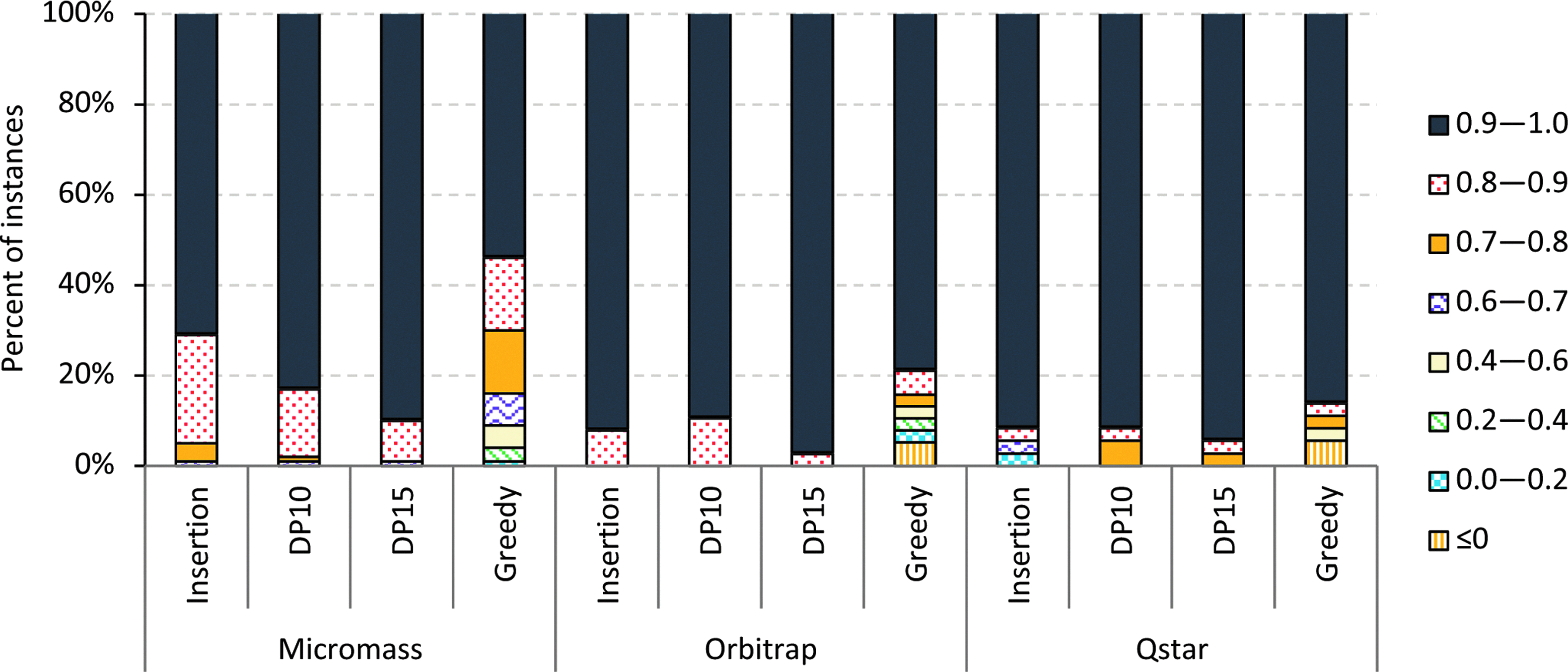
Performance ratios achieved by different heuristics on Micromass, Orbitrap, and QSTAR datasets.

FIG. 4.

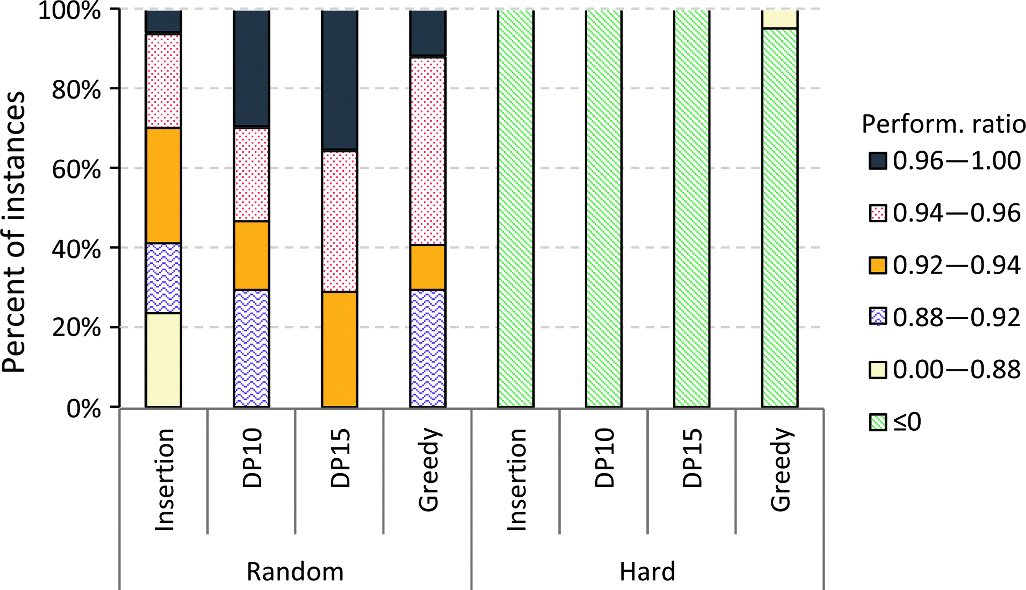
Performance ratios achieved by different heuristics on Random and Hard datasets.

The insertion heuristic performs better than the greedy heuristic in our experiments on real datasets, while on the Random dataset, the greedy heuristic generates trees with better scores. All heuristics completely fail on the Hard dataset, where most of the time they return the empty tree as output. We also observe improved performance in general for the tree completion heuristic as we increase the parameter (i. e., the size of the backbone computed exactly). But the performance increase is only marginal for real-world datasets, as can be seen in Figures 3 and 4. The tree completion heuristic becomes infeasible when the size of the backbone is 25. In this case, more than half of the instances from Orbitrap and Micromass datasets fail to terminate in less than a week.

The insertion, greedy, and DP₁₀ heuristics are fast with running times well under a second, whereas the DP₁₅ heuristic terminates in less than 8 seconds for all instances. The algorithm based on integer programmming also finished in, at most, 16 seconds for any instance, while it was actually faster on most of the instances. Both integer programming solvers showed comparable performance except on the Hard instances, where CPLEX was noticeably slower than the Gurobi solver. Figures 5 and 6 present the breakdown of datasets depending on how much time it took to solve them using different algorithms. Note that the running times mentioned do not include the time needed to construct the graph representations from MS data.

FIG. 5.

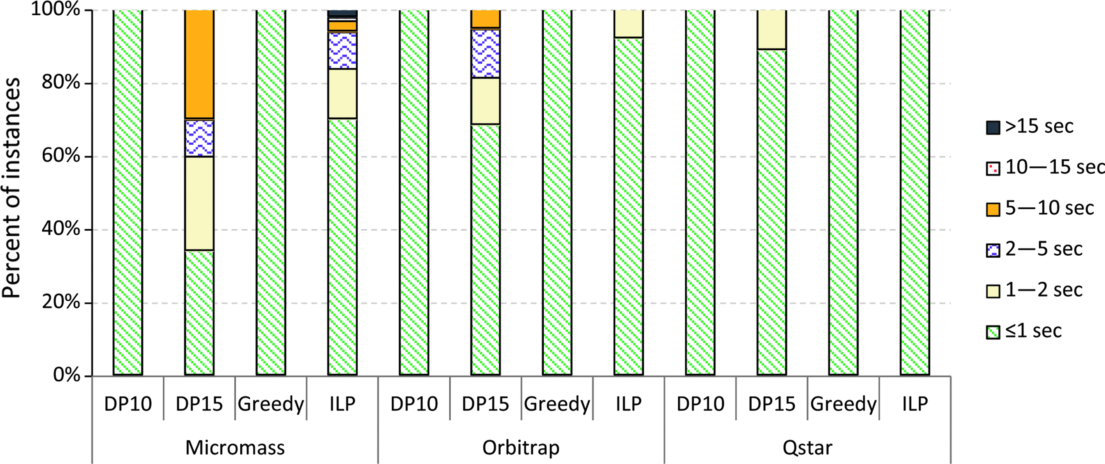
Running times taken by different heuristics on Micromass, Orbitrap, and QSTAR datasets, where (ILP) denotes the algorithm based on integer programming with Gurobi solver.

FIG. 6.

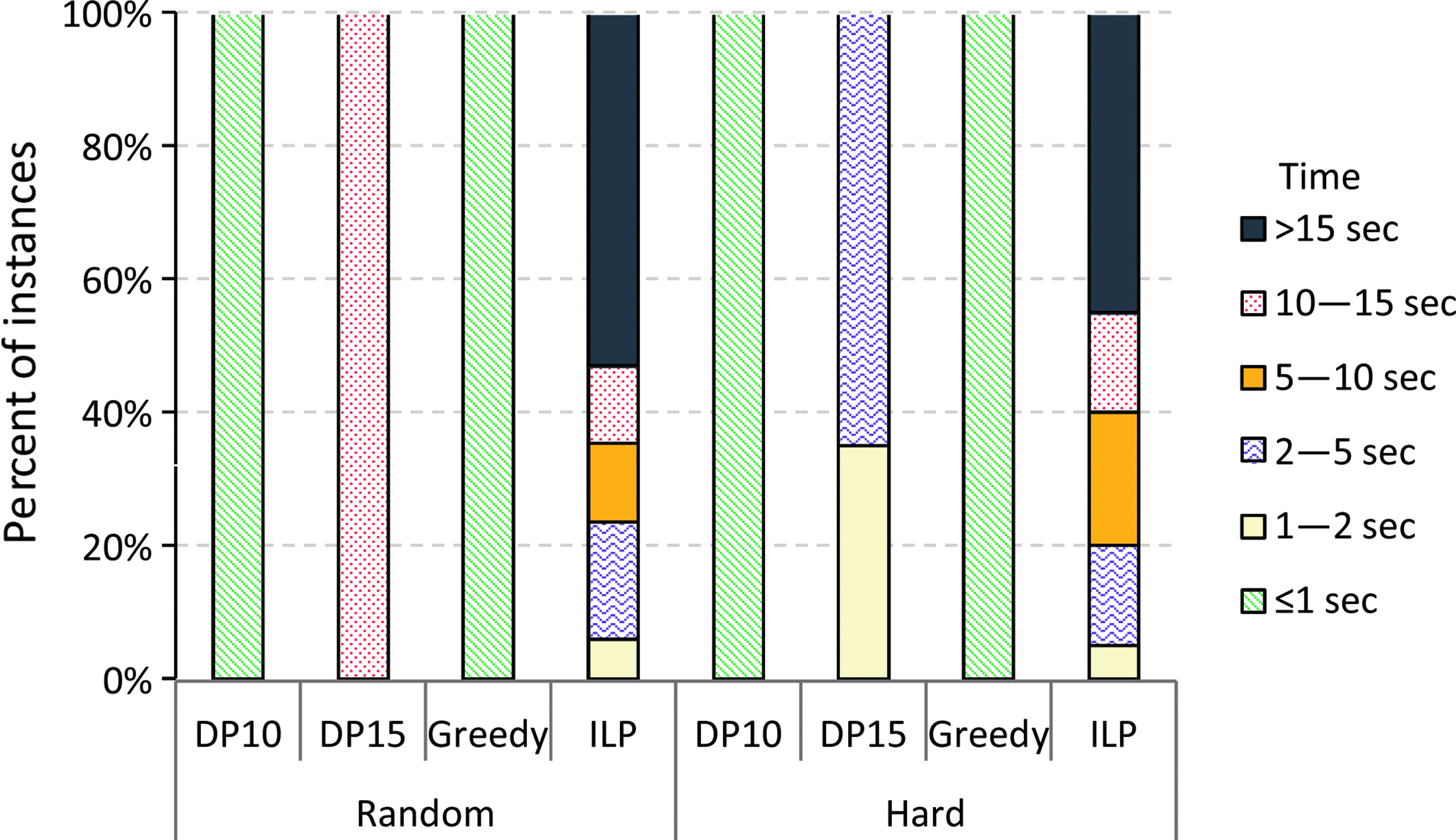
Running times taken by different algorithms on Random and Hard datasets, where ILP denotes the algorithm based on integer programming with Gurobi solver.

6. Conclusions

We have discussed several exact and heuristic algorithms for the Maximum Colorful Subtree problem, and also shown its inapproximability even for colorful input graphs. The Maximum Colorful Subtree problem is relevant for the de novo analysis of metabolite mass spectra.

Experiments on five different sets of graphs from actual metabolite spectra and randomly generated graphs reveal that, for smaller test instances, the brute force and dynamic programming-based algorithms can calculate the optimal solution quickly. When the structure of the fragmentation tree is of interest, for example, for tree alignment (Hufsky, 2012a; Rasche et al., 2012), it is most probably beneficial to find exact solutions. Our tests show that the integer linear program performs best on this task. When determining the sum formula, hundreds of instances have to be solved for a single compound, but only the scores are relevant. In this case, the tree completion heuristic with parameter 10 provides a good performance ratio of 95% on average, as well as very fast running times. Increasing the parameter did increase the quality of results, but at the price of highly increased running times.

Expert evaluations in Rasche et al. (2011) and Hufsky et al. (2012b) indicate that trees with optimal objective function are structurally reasonable. Thus, we conjecture that this is generally the case, but, of course, we cannot guarantee that the tree with optimal objective function is the “true” tree. This is true for most problems in computational biology, however, so we deliberately ignored this fact.

Fast calculation of fragmentation trees is a prerequisite for the identification of unknown metabolites from fragmentation mass spectra. It is required for molecular formula identification (Rasche et al., 2011) and the classification of unknowns using fragmentation tree alignment (Rasche et al., 2012). The algorithms presented here can play an integral role in this fully automated pipeline.

In the future, we intend to test whether “advanced” ILP techniques, such as branch-and-cut or column generation, will further decrease running times. It also remains open whether a modified version of the ILP can solve the (presumably even harder) Colorful Subtree Closure instances (Scheubert et al., 2011) in reasonable time.

Footnotes

Acknowledgments

I.R. thanks Tsuyoshi Ito for giving the first idea of the proof of Theorem 1 (Ito, ). Kerstin Scheubert suggested a simplification in the proof. We thank Aleš Svatoš (Max Planck Institute for Chemical Ecology in Jena, Germany), Christoph Böttcher (Institute for Plant Biochemistry in Halle, Germany), and David Grant (University of Connecticut in Storrs, Connecticut) for supplying us with the test data.

Author Disclosure Statement

S.B. and F.R. are co-inventors of an international patent concerning the comparison of fragmentation trees. The other co-authors declare that no competing financial interests exist.

1

Gurobi Optimizer 4.5. Houston, Texas: Gurobi Optimization Inc., April 2011.

2

IBM ILOG CPLEX Optimization Studio 12.3. Armonk, New York: IBM Corporation, June 2011.

References

Björklund

, Husfeldt

, Kaski

, Koivisto

2007. Fourier meets Möbius: fast subset convolution. Proc. of ACM Symposium on Theory of Computing (STOC 2007) ACM Press: New York, 67–74.

Böcker

, Rasche

2008. Towards de novo identification of metabolites by analyzing tandem mass spectra. Bioinformatics, 24:I49–I55.

Dondi

, Fertin

, Vialette

2009. Maximum motif problem in vertex-colored graphs. Proc. of Symposium on Combinatorial Pattern Matching (CPM 2009), Lect. Notes Comput. Sci., 5577. Springer: Berlin, 221–235.

Dreyfus

S.E.

, Wagner

R.A.

1972. The Steiner problem in graphs. Networks, 1:195–207.

Fellows

M.R.

, Gramm

, Niedermeier

2006. On the parameterized intractability of motif search problems. Combinatorica, 26:141–167.

Fernie

A.R.

, Trethewey

R.N.

, Krotzky

A.J.

, Willmitzer

2004. Metabolite profiling: from diagnostics to systems biology. Nat. Rev. Mol. Cell Biol., 5:763–769.

Guillemot

, Sikora

2010. Finding and counting vertex-colored subtrees. Proc. of Mathematical Foundations of Computer Science (MFCS 2010), Lect. Notes Comput. Sci., 6281. Springer: Berlin, 405–416.

Hill

D.W.

, Kertesz

T.M.

, Fontaine

et al. 2008. Mass spectral metabonomics beyond elemental formula: Chemical database querying by matching experimental with computational fragmentation spectra. Anal. Chem., 80:5574–5582.

Hufsky

, Dührkop

, Rasche

et al. 2012a. Fast alignment of fragmentation trees. Bioinformatics, 28:i265–i273Proc. of Intelligent Systems for Molecular Biology (ISMB 2012).

10.

Hufsky

, Rempt

, Rasche

et al. 2012. De novo analysis of electron impact mass spectra of metabolites using fragmentation trees. Anal. Chim Acta., 739:67–76.

11.

Ito

2011. Finding maximum weight arborescence in an edge-weighted DAG. http://cstheory.stackexchange.com/q/4088/189. 2011 Oct 12.

12.

Koutis

, Williams

2009. Limits and applications of group algebras for parameterized problems. Proc. of International Colloquium on Automata, Languages and Programming (ICALP 2009), Lect. Notes Comput. Sci., 5555. Springer: Berlin, 653–664.

13.

J.W.-H.

, Vederas

J.C.

2009. Drug discovery and natural products: end of an era or an endless frontier? Science, 325:161–165.

14.

Ljubić

, Weiskircher

, Pferschy

et al. 2005. Solving the prize-collecting steiner tree problem to optimality. Proc. of Algorithm Engineering and Experiments (ALENEX 2005) SIAM: Philadelphia, 68–76.

15.

Oberacher

, Pavlic

, Libiseller

et al. 2009. On the inter-instrument and inter-laboratory transferability of a tandem mass spectral reference library: 1. results of an Austrian multicenter study. J. Mass Spectrom., 44:485–493.

16.

Rasche

, Scheubert

, Hufsky

et al. 2012. Identifying the unknowns by aligning fragmentation trees. Anal. Chem., 84:3417–26.

17.

Rasche

, Svatoš

, Maddula

R.K.

et al. 2011. Computing fragmentation trees from tandem mass spectrometry data. Anal. Chem., 83:1243–1251.

18.

Scheubert

, Hufsky

, Rasche

, Böcker

2011. Computing fragmentation trees from metabolite multiple mass spectrometry data. J. Comput. Biol., 18:1383–1397.

19.

Sikora

2010. An (almost complete) state of the art around the graph motif problem. Technical report. Université Paris-Est: France www-igm.univ-mlv.fr/∼fsikora/pub/GraphMotif-Resume.pdf

20.

Sikora

2011. Aspects algorithmiques de la comparaison d'éléments biologiques. [PhD thesis] Université Paris-Est: France.

21.

, Li

2006. Many hard examples in exact phase transitions. Theor. Comput. Sci., 355:291–302.