Detecting Phylogenetic Signals in Eukaryotic Whole Genome Sequences

Abstract

Whole genome sequences are a rich source of molecular data, with a potential for the discovery of novel evolutionary information. Yet, many parts of these sequences are not known to be under evolutionary pressure and, thus, are not conserved. Furthermore, a good model for whole genome evolution does not exist. Consequently, it is not a priori clear if a meaningful phylogenetic signal exists and can be extracted from the sequences as a whole. Indeed, very few phylogenies were reconstructed based on these sequences. Prior to this work, only two reconstruction methods were applied to large eukaryotic genomes: the K_r method (Haubold et al., 2009), which was applied to genomes of rather small diversity (Drosophila species), and the feature frequency profile method (Sims et al., 2009a), which was applied to genomes of moderate diversity (mammals).

We investigate the whole genome-based phylogenetic reconstruction question with respect to a much wider taxonomic sample. We apply K_r, FFP, and an alternative alignment-free method, the average common subsequence (ACS) (Ulitsky et al., 2006), to 24 multicellular eukaryotes (vertebrates, invertebrates, and plants). We also apply ACS to the proteome sequences of these 24 taxa. We compare the resulting trees to a standard reference, the National Center for Biotechnology Information (NCBI) taxonomy tree. Trees produced by ACS_AA, based on proteomes, are in complete agreement with the NCBI tree. For the genome-based reconstruction, ACS_DNA produces trees whose agreement with the NCBI tree is excellent to very good for divergence times up to 800 million years ago, medium at 1 billion years ago, and poor at 1.6 billion years ago. We conclude that whole genomes do carry a clear phylogenetic signal, yet this signal “saturates” with longer divergence times. Furthermore, from the few existing methods, ACS is best capable of detecting this signal.

1. Introduction

Whole genome sequences are a rich source of molecular data, with a potential for the discovery of novel evolutionary information. Yet, so far they've hardly been used to reconstruct phylogenetic trees, especially for multicellular eukaryotes. Genomes of multicellular eukaryotes are mostly composed of sites not coding for proteins. It is not at all clear in advance if the genomes of a wide set of such species have not diverged too much to carry any detectable phylogenetic signal.

Sequencing technology has greatly improved over the last decade. As a result, we now have at our disposal over 1,500 complete genomic sequences, including 153 Eucaryotic genomes, according to GOLD on-line database (Liolios et al., 2010), accessed December, 2010. Complete genomes contain many evolutionary signals beyond those in protein coding genes, but for the most part we are either not aware of them or cannot detect them. Processing whole eukaryotic genomes, especially large ones, necessitates strong computers with large memory capacity. Such computers are now available at a moderate cost. Consequently, we are now in the unique position of having access to the genomic sequences and the computational infrastructure to process and analyze them.

Molecular sequence–based phylogenetic reconstruction is traditionally built upon small molecular sequences such as proteins or protein coding genes. Most reconstruction methods (both amino acid and DNA), like Maximum Likelihood (Felsenstein, 1981), Maximum Parsimony (Eck and Dayhoff, 1966; Fitch, 1977), and Minimum Evolution (Saitou and Imanishi, 1989), as well as the computation of pairwise distances among sequences, start by aligning the input sequences. This makes sense when they are short, homolog sequences. But when dealing with different types of biological sequences, especially whole genomes, alignment becomes problematic. Recombination, shuffling, and rearrangements, acting on medium and large scales, yield noncollinear genomes. Furthermore, substantial length differences between genomes of different species imply that any pairwise or multiple alignment will be dominated by noninformative gaps. The obstacles for alignment-based phylogenetic reconstruction motivated several alignment-free methods in recent years (Stuart et al., 2002a,b; Otu and Sayood, 2003; Qi et al., 2004; Ulitsky et al., 2006; Höhl et al., 2006; Apostolico and Denas, 2008; Haubold et al., 2009; Sims et al., 2009a,b; Apostolico et al., 2010). Still, the majority of these alignment-free methods were applied only to moderate-size sequences (a few hundred thousand bases)—either genomic or simulated—and seem not to be applicable to much longer sequences. The methods of Qi et al. (2004) and Apostolico et al. (2010) were applied to unicellular species with small genomes (including archaea, bacteria, and eukarya).

So far, the only method that was actually applied to the genomic sequences of diverged multicellular eukaryotes is the feature frequency profile (FFP) method (Sims et al., 2009a,b). In Sims et al. (2009b), FFP was applied to 10 different mammalian genomes, ranging from human to platypus. Whole genome sequences, intronic regions sequences, exonic regions sequences, and nongenic regions sequences were separately considered. The four resulting trees were slightly different, but essentially all were in good agreement with the “accepted tree” for these species (Murphy et al., 2001; Nikolaev et al., 2007; Prasad et al., 2008). The work of Sims et al. (2009a,b) has demonstrated, for the first time, the viability of the whole-genome approach for phylogenetic reconstruction in mammals.

Haubold et al. (2009) designed the K_r measure, which is closely related to the average common subsequences (ACS) measure (Ulitsky et al., 2006). K_r is primarily intended for alignment-free comparison of closely related sequences. It was successfully applied to the genome sequences of 12 Drosophila species. Haubold et al. (2009) report that the resulting tree fully agreed with the accepted reference tree of these 12 species and that ACS produces a different tree than the reference tree of the same 12 species. We ran our ACS implementation over the same dataset, and the outcome was in perfect agreement with the accepted reference tree. A possible source of the discrepancy is the use of single strand versions of the flies genome sequences by Haubold et al., vs. the use of both strands in our implementation.

In this work, we investigate this question with respect to a much wider taxonomic sample. We apply FFP, as well as the ACS method, to double-stranded, whole genome sequences of 24 multicellular eukaryotes, which include 12 vertebrates (9 tetrapods and 3 bony fish), 7 invertebrates (1 sea squirt, 4 insects, and 2 worms), and 5 plants. We also apply ACS to the proteome sequences of these 24 taxa. Both FFP and ACS methods can be applied to whole genomes (or to specific parts). The sequences need not share a common set of genes, and no syntenic map (Liao et al., 2004) or partial alignment is required. ACS has already been applied earlier to whole proteome sequences. For all these 24 species, we used the publicly available genome and proteome sequences.

We compare the resulting trees to a standard reference tree–the National Center for Biotechnology Information (NCBI) taxonomy tree (Sayers et al., 2009; Benson et al., 2009). We comment that there is no single, universally accepted reference tree, as there are some disputed clades. For example, an ongoing question is whether nematodes are an outgroup of the insects and chordata within the metazoa—the Coelomata hypothesis (Hyman, 1940), which was the dominant view for decades—or whether the nematodes and insects form a clade within the metazoa—the more recent Ecdysozoa hypothesis (Dunn et al., 2008; Holton and Pisani, 2010). We note that the NCBI tree supports the former hypothesis. Clearly, no tree, whole genome based or not, can be compatible with different, incompatible reference trees.

Our proteome-based ACS reconstruction for these 24 eukaryotes yields phylogenetic trees that are in perfect agreement with the NCBI taxonomy tree. For genome-based reconstruction, the extent of the agreement depends on the (estimated) divergence times within the set of taxa. When the divergence time is less than 800 million years ago, the resulting trees agree with the reference tree. When the divergence time exceeds one billion years ago, the resulting trees deviate substantially from the NCBI taxonomy tree and from the common views in general.

2. Methods

2.1. Data sources

We selected a group of eukaryotic species with large genome sequences, ranging from 87Million base pairs (Mbp) (Brugia malayi) to 3,500Mbp (Monodelphis domestica), such that both their genome and proteome are publicly available. These include 12 vertebrates (Anolis carolinensis, Danio rerio, Gallus gallus, Homo sapiens, Monodelphis domestica, Mus musculus, Ornithorhynchus anatinus, Oryzias latipes, Pan troglodytes, Rattus norvegicus, Taeniopygia guttata, and Takifugu rubripes), 1 urochordata (Ciona intestinalis), 4 insects (Anopheles gambiae, Apis mellifera, Drosophila melanogaster, and Tribolium castaneum), 2 nematodes (Brugia malayi and Caenorhabditis elegans), and 5 plants (Arabidopsis lyrata, Arabidopsis thaliana, Oryza sativa, Populus trichocarpa, and Zea mays). The two Arabidopsis species are included in the study as a “sanity check.” Since their divergence time is similar to the human–chimp, they are very close in evolutionary terms.

All the genomes and proteomes were downloaded from NCBI (Pruitt et al., 2007), except Anolis carolinensis, Oryzias latipes, and Takifugu rubripes, whose genomes were downloaded from UCSC (Kuhn et al., 2009), and whose proteomes were downloaded from ENSEMBL (Hubbard et al., 2009), and the genome of Arabidopsis lyrata, which was downloaded from JGI (Grigoriev et al., 2012). The four databases were accessed early in 2009.

For each species, we concatenated all the chromosomes using a special “stop character” between them. The gaps in the DNA sequences (a sequence of consecutive Ns) were replaced by the same “stop character.” In addition, we concatenated the reverse complement to form the reference DNA genome. Based on these references—four-state DNA genomes—we compiled the two-state purine-pyrimidine (RY) genomes of the 24 species. The proteome of each species was created by concatenating all its RefSeq proteins (Pruitt et al., 2009), where applicable, separated by a special “stop character.”

2.2. Algorithms and tools

ACS is a nonparametric method for alignment-free genome comparison. It is based on finding locally maximal common substrings among pairs of sequences, which could be over any alphabet, in particular four-state DNA, two-state RY, or twenty-state amino acid (AA) sequence. It employs suffix arrays and, unlike the parametric FFP, it does not filter out any low complexity (or other) portions of the input sequences. The ACS implementation requires substantial computational resources, both primary, high speed memory (RAM) and computation time. We used a Linux machine with 64GB RAM, and in our current implementation the comparison of two large genomes takes about two hours. Smaller amount of primary memory will result in a noticeable performance slowdown.

Our ACS implementation is a modification of the ACS original code, which was supplied by its authors. The modified code speeds up the running time of the suffix array search. We were not able to obtain a complete running code of FFP, so we have coded it ourselves, following the description in Sims et al. (2009a). We used the block FFP version of the algorithm, as the lengths' ratios between the longest and shortest genomes are up to thirty-five-fold. We used word filtering (respective to their complexity and frequency) and the word size that was recommended in Sims et al. (2009a,b). ACS was applied to the DNA genomic sequences, to the AA proteome sequences, and to the compiled RY genomic sequences. FFP was applied to the compiled RY genomic sequences, exactly as prescribed in Sims et al. (2009a,b).

In order to quantify the difference between a computed tree and our benchmark tree, the Robinson–Foulds (RF) (Robinson and Foulds, 1981) metric was used. The RF distance between two trees (with the same taxa set) is the number of bi-partitions of taxa implied by the first tree but not the second tree, plus the number of bi-partitions implied by the second tree but not the first tree.

In addition to the different variants of ACS and FFP, we have also tried computing pairwise distances using the K_r method. The published K_r code required memory exceeding the 64GB RAM on our machine. Employing a modification of our ACS implementation, together with parts of the original K_r code, resulted in an implementation that consumes less memory and converged with bounded values for most pairs of species. Yet in all clades we have considered (see Section 3), there was at least one pair of species for which the modified code did not converge to a bounded value. Therefore, it was not possible to reconstruct phylogenetic trees using our implementation of K_r for any set of taxa considered here.

We have used the following leave one out (LOO) stability measure for phylogenetic trees based on distance matrices. We are given an n species, n-by-n distance matrix, and a neighbor joining (NJ) tree (Saitou and Nei, 1987) resulting from it, which we term the original tree. The following process is repeated n times, once for each of the n species: We remove the row and column corresponding to this species from the n-by-n distance matrix. This results in a new, (n − 1)-by-(n − 1), distance submatrix. We run NJ on this submatrix and get an n − 1 species tree as a result, termed the query tree. Next, we remove the same species from the original tree and contract redundant edges. The resulting tree is termed the induced tree. We compute the RF score of the query tree vs. the induced tree. We average the resulting n RF scores. This average is defined as the LOO score of the n-by-n distance matrix. The lower this LOO score is, the more stable the distances with respect to NJ reconstruction.

We have used the Phylogeny Inference Package (PHYLIP) (Felsenstein, 1989) to compute the NJ trees, and the Interactive Tree Of Life (iTOL) web-based tool (Letunic and Bork, 2007) to plot the phylogenetic figures. Figure 1 shows the superposition of divergence times (based on the online database TIMETREE; Hedges et al., 2006) on the NCBI taxonomy tree. We remark that for the 24 species studied here, estimated divergence times (averages over several references) of the metazoa, the chordata and insects, and the insects and nematodes are all 1 billion years ago (bya).

FIG. 1.

Superimposing divergence times on NCBI taxonomy tree. The numbers indicate the divergence times in units of million years ago (mya). The divergence times are based on a simple average of several estimations which are usually ± 10% of the reported number.

Availability: The ACS code used in this work is available upon request. We note that running it on large eukaryotic genomes requires at least 50GB of available RAM.

3. Results

We used both FFP and ACS to compute distances, based on either the four-state DNA genome sequence, the reduced, two-state RY genome sequence, or the AA proteome sequence, as applicable. For FFP, only the RY sequences were used, following the specifications in Sims et al. (2009a,b). For ACS, we used four-state DNA, RY, and AA proteome sequences. The resulting combinations are denoted ACS_DNA, FFP_RY, ACS_RY, and ACS_AA, correspondingly. We applied NJ to construct trees from the resulting distance matrices, and then rooted the trees using accepted outgroups. For the ACS_DNA and the ACS_RY, the resulting edge weights were mostly not meaningful, thus, unweighted neighbor joining (UNJ) (Gascuel, 1997) was used. The reason for that stems from the small difference among the ACS_DNA and ACS_RY pairwise distances. For example, all the pairwise ACS_DNA distances are in the range 1.80–2.08, except for the human–chimp (0.39), the two arabidopsis (1.53), and the mouse–rat (1.63). By way of contrast, edge lengths produced by NJ on ACS_AA data were meaningful, thus, the tree in Figure 8 displays weighted edges.

We analyzed the results on the set of 24 taxa, as well as on different subsets that represent taxonomic clades. While most of these clades, such as plants, mammals, tetrapods, vertebrates, chordata, or metazoa, are commonly agreed upon, others are still a subject of debate. We performed our analysis on the set of all 24 species, on the 6 clades mentioned above, and on 2 disputed clades: insects and nematodes, and chordata and insects (Table 1).

Table 1.

Qualitative Description and Robinson-Foulds Score of the Agreement with the NCBI Taxonomy Tree for Each Reconstruction Method and Clade

			RF score with respect to benchmark				LOO score
Clade	No. of species	Div. time (mya)	ACS_AA	ACS_DNA	ACS_RY	FFP_RY	ACS_DNA
Plants	5	230	excellent	excellent	excellent	excellent	0.5
				0	0	0	0
Mammals	6	220	excellent	excellent	excellent	excellent	0/6 = 0
			0	0	0	0
Tetrapods	9	320	excellent	very good	very good	good	0/9 = 0
			0	2	2	4
Vertebrates	12	450	excellent	very good	very good	medium	0/12 = 0
			0	4	2	8
Chordata	13	800	excellent	very good	very good	poor	4/13 = 0.31
			0	4	4	10
Insects and nematodes^a	6	1000	excellent	excellent	poor	poor	4/6 = 0.67
			1^b	1^b	3	3
Chordata and Insects	17	1000	excellent	good	medium	poor	14/17 = 0.82
			0	9	11	17
Metazoa	19	1000	excellent	medium	poor	poor	2/19 = 0.11
			0	13	15	19
All	24	1600	excellent	poor	poor	poor	38/24 = 1.58
			0	23	23	23

Not a clade in the NCBI taxonomy tree.

RF score is 1 as the reference tree is not fully resolved; yet these fully resolved ACS trees are compatible with the reference tree.

Last column, “LOO Score,” describes the stability of the ACS_DNA trees.

NCBI, National Center for Biotechnology Information; Mya, million years ago; RF score, Robinson-Foulds score; LOO, leave one out.

The resulting ACS_DNA trees of two clades agree perfectly with the NCBI taxonomic tree. These clades are the five plants (Fig. 2, divergence time 230 million years ago [mya]), and six mammals (divergence time 220 mya). The ACS_DNA tree (Fig. 3) of the four insects and two nematodes (divergence time 1,000 mya) also agree. This species set is not a clade according to the NCBI taxonomy tree, but as we discussed above, it is considered a clade by the Ecdysozoa hypothesis.

FIG. 2.

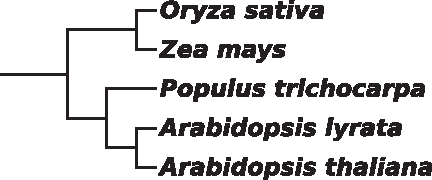
Unweighted NJ tree for ACS_DNA for the group of five plants.

FIG. 3.

Unweighted NJ tree for six invertebrates (insects and nematodes), based on ACS_DNA distances.

The ACS_DNA tree of the 12 vertebrates (Fig. 4, divergence time 450 mya) and the chordata clade Ciona intestinalis, plus the vertebrates (Fig. 5, divergence time 800 mya), are in very good agreement with the NCBI taxonomic tree. In both cases, Anolis carolinensis is misplaced as an outgroup of the tetrapods. This contradicts the modern view that birds and reptiles (diapsids) are a clade, and synapsids (mammals) versus diapsids is the basal divergence in amniotes (Kardong, 2009).

FIG. 4.

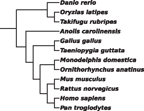
Unweighted NJ tree for the 12 vertebrates, based on ACS_DNA distances.

FIG. 5.

Unweighted NJ tree for the 13 taxa chordata clade, based on ACS_DNA distances.

Adding the two nematodes and four insects to the chordata clade gives us the metazoan clade. The resulting ACS_DNA tree (Fig. 6) deviates in several details from the NCBI taxonomy tree. The vertebrates are grouped as a separate clade, and their inner organization is good—only Danio rerio and Anolis carolinensis are misplaced. They were supposed to be an outgroup of the fish and birds, respectively.) However, Ciona intestinalis is placed among the insects instead of being an outgroup of the vertebrates. Moreover, the nematodes are placed among the insects instead of being an outgroup of them. The 24-species ACS_DNA tree, which includes the five plants in addition to the metazoan clade (Fig. 7, divergence time 1.6 bya), substantially deviates from all accepted trees. The plants are not clustered together, and, in particular, maze is placed among tetrapods and rice among vertebrates. For the mammals, tetrapods and chordata–insects clades, the corresponding trees produced by ACS_DNA are depicted in Supplementary Figs. S1–S3 (Supplementary Material is available online at www.liebertonline.com/cmb).

FIG. 6.

Unweighted NJ tree for 19 metazoan, based on ACS_DNA distances.

FIG. 7.

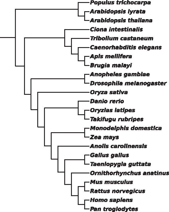
Unweighted NJ tree for the 24 species, based on ACS_DNA distances.

By way of contrast, the ACS_AA tree on all 24 taxa (Fig. 8), as well as the ACS_AA trees on all species sets mentioned earlier, fully agree with the NCBI taxonomy tree (the latter is not fully resolved, while the ACS_AA tree is, yet, they are compatible). Thus, the ACS_AA support the Coelomata theory.

FIG. 8.

Weighted NJ tree for all 24 species, based on ACS_AA distances.

For almost all subsets of species discussed above, the FFP_RY and ACS_RY trees demonstrate a smaller or equal agreement with the NCBI taxonomy tree than the ACS_DNA trees. The only exception is the vertebrates clade, where the tree produced by ACS_RY demonstrates a higher agreement than the trees produced by ACS_DNA and FFP_RY. The FFP_RY and ACS_RY trees are depicted in Supplementary Figs. S4–S21. Table 1 summarizes the results of each method and clade, describing them both verbally and quantitatively, using the Robinson-Foulds (RF) score with respect to the NCBI taxonomy tree.

We have checked the stability of the resulting ACS_DNA trees using the LOO score (see last column in Table 1). For the trees of plants, mammals, tetrapods, and vertebrates, the LOO score equals zero. The trees of chordata, insects and nematodes, chordata and insects, and metazoa have scores 4/13, 4/6, 14/17, and 2/19 respectively. The tree with all the 24 species has a LOO score of 38/24.

4. Discussion

The vast majority of sites in the genomes of multicellular eukaryotes are not coding for proteins. Even if known RNA genes, promotors, and other known functional elements are taken into account, they cover only a small fraction of the genome. Consequently, it is not clear what evolutionary constraints are imposed on most of the genome, if any, and to what extent it is free to evolve under weak or no constraints. Therefore, it is not at all obvious, a priori, if the genomes of a diverse set of multicellular eukaryotes have not diverged too much to carry any detectable phylogenetic signal. Sims et al. (2009a,b) showed that FFP_RY can detect such signal for a set of mammalian genomes. We showed that ACS_DNA can detect a strong signal over the vertebrate, chordata, and plant clades, producing unweighted trees of very good quality. This signal is not evident (and, for example, does not support the reconstruction of weighted trees), but it does exist, and ACS_DNA detects it. The signal, as detected by ACS_DNA, exists over the metazoan clade but it deteriorates, and it essentially fades over the set of 24 species that includes both metazoa and plants.

Both ACS_AA and ACS_DNA reconstruction methods work very well over the vertebrate, chordata, and plant clades. These clades are characterized by medium divergence times (450, 800, 230 mya, correspondingly) and by a substantial range of genome sizes (350 to 3,500 million bases for vertebrates, 113 to 3,500 for chordata, 120 to 1,900 for plants). However, the very good agreement with the accepted phylogenetic history deteriorates when applying ACS_DNA to metazoa (divergence time 1,000 mya and genome sizes from 87 to 3,500 million bases), and it completely breaks down when applied to the combined set of 24 species—vertebrates, invertebrates, and plants (divergence time of 1,600 mya). Interestingly, ACS_AA performs perfectly, relative to the NCBI tree1, for metazoa, all 24 species, and all other seven clades. We remark that neither FFP_RY nor ACS_RY fared any better with respect to either metazoa or all 24 species. Our results indicate that existing whole genome methods, those which can be applied to large eukaryotic genomes, yield trees that substantially deviate from the common evolutionary understanding when the taxa set includes both animals and plants. There is a clear relation between quality of the trees (agreement with the benchmark) and its stability score (by the LOO measure).

We do not expect whole genome reconstruction methods to produce trees that are in perfect agreement with the taxonomic tree. Genomes undergo processes that are not experienced at the protein coding gene or RNA gene levels. Yet, a tree interleaving plants and animals in the same clade is not acceptable. Since applying ACS_DNA to most clades separately produced good outcomes, we concluded that the intra clade distances give rise to correct trees via the NJ algorithm, and the inter clade distances cause the incorrect outcome.

One could conjecture that QC-content (Guyon et al., 2009) and/or genome length could bias the resulting tree. Figure 9 shows the GC content and genome lengths, superimposed over the ACS_DNA tree. Sister taxa in the tree differ substantially with respect to these two factors, and overall the tree is not correlated with them.

FIG. 9.

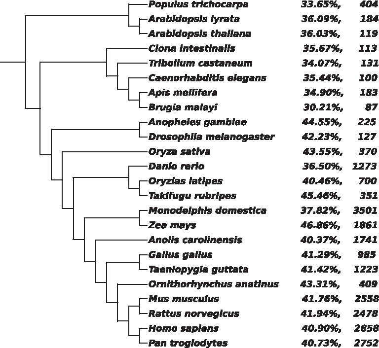
Superimposing QC-content and genome length on the ACS_DNA tree. Each label contains the percentage of GC content and the genome length (after omitting repeated Ns) in Mbp.

Clades with relatively recent divergence times were constructed well, while the set of all 24 species gave rise to a low-quality tree. This outcome is somewhat counterintuitive: We could expect interclade distances to be large enough to support distinct clustering of different clades, but this turned out not to be the case.

The ACS_AA-based tree represents, to some degree, the general “proteome view.” The fact that this coincides with the NCBI taxonomy tree indicates that the variety of criteria underlying its construction agree with this general “proteome view.”

5. Conclusion

For short homolog genomic sequences, such as genes, highly established methods for detecting phylogenetic signals and building trees exist. Whole genome sequences clearly contain all this information and much more. Still, whole genomes have gone through complex processes that are only partially understood, and it is not a priori clear if coherent phylogenetic signal can be extracted from them as a whole. Alignment-free methods for sequence comparison are attempting to achieve this goal. However, the search for a good alignment-free whole genome distance method is still in its infancy, with the FFP being the first and the present, ACS based work being just the second to tackle large genomes (K_r being inapplicable at these evolutionary ranges).

ACS and FFP already seem to affirmatively resolve the fundamental question, “Do whole genomes carry a detectable phylogenetic signal?” With the two existing reconstruction methods, the affirmative answer depends on estimated divergence times, and when it exceeds 800 mya, the signal seems to gradually degrade or become saturated. ACS seems to be the more accurate of the two methods for all clades but the one with the longest divergence times, where both methods do poorly. It is possible that future, more refined reconstruction methods will be able to recover the signal deeper into the past. Future research should also address additional issues, such as estimating branch lengths, devising accurate distance measures for close and distant species, and providing a good methodology to validate the outcomes.

Footnotes

Acknowledgments

Thanks to David Burstein for supplying the original ACS code and to Ilan Grunau, Micha Ilan, Shai Meiri, and Nimrod Rubinstein for helpful discussions. E.C. was supported in part by a fellowship from the Edmond J. Safra Bioinformatics program at Tel-Aviv University. The research of B.C. was not supported by the Israeli Science Foundation (ISF) or any other funding agency.

Disclosure Statement

No competing financial interests exist.

1

Thus, it is compatible with the Coelomata hypothesis.

References

Apostolico

, Denas

2008. Fast algorithms for computing sequence distances by exhaustive substring composition. Algorithms Mol. Biol., 3:13.

Apostolico

, Denas

, Dress

2010. Efficient tools for comparative substring analysis. J-Biotechnol., 149:120–126.

Benson

D.A.

, Karsch-Mizrachi

, Lipman

D.J.

et al. 2009. Genbank. Nucleic Acids Research, 37:D26–31.

Dunn

C.W.

, Hejnol

, Matus

D.Q.

et al. Broad phylogenomic sampling improves resolution of the animal tree of life. Nature, 452:745–749.

Eck

R.V.

, Dayhoff

M.O.

1966. Atlas of Protein Sequence and Structure. National Biomedical Research Foundation: Silver Spring, Maryland.

Felsenstein

1981. Evolutionary trees from dna sequences: a maximum likelihood approach. J. Mol. Evol., 17:368–376.

Felsenstein

1989. Phylip–phylogeny inference package. Cladistics, 5:164–166.

Fitch

1977. On the problem of discovering the most parsimonious tree. The American Naturalist, 111:223–257.

Gascuel

1997. Concerning the nj algorithm and its unweighted version, unj, 149–170. Mirkin

, McMorris

F.R.

, Roberts

F.S

et al. Mathematical Hierarchies and Biology, 37. American Mathematical Society and DIMACS Series in Discrete Mathematics and Theoretical Computer Science: Providence, RI.

10.

Gigoriev

I.V.

, Nordberg

, Shabalov

et al. 2012. The Genome Portal of the Department of Energy Joint Genome Institute. Nucleic Acids Res., 40:D26–32.

11.

Guyon

, Brochier-Armanet

, Guénoche

2009. Comparison of alignment free string distances for complete genome phylogeny. Advances in Data Analysis and Classification, 3:95–108.

12.

Haubold

, Pfaffelhuber

, Domazet-Loso

et al. 2009. Estimating mutation distances from unaligned genomes. J. Comput. Biol., 16:1487–500.

13.

Hedges

S.B.

, Dudley

, Kumar

2006. Timetree: a public knowledge-base of divergence times among organisms. Bioinformatics, 22:2971–2972.

14.

Höhl

, Rigoutsos

, Ragan

M.A.

2006. Pattern-based phylogenetic distance estimation and tree reconstruction. Evol. Bioinform. Online, 2:359–375.

15.

Holton

T.A.

, Pisani

2010. Deep genomic-scale analyses of the metazoa reject coelomata: evidence from single- and multigene families analyzed under a supertree and supermatrix paradigm. Genome Biol. Evol., 2:310–24.

16.

Hubbard

T.J.

, Aken

B.L.

, Ayling

, Ballester

et al. 2009. Ensembl 2009. Nucleic Acids Res., 37,Database:D690–7:D690–7.

17.

Hyman

L.H.

1940. The Invertebrates: McGraw Hill, New York.

18.

Kardong

K.V.

2009. Vertebrates: Comparative anatomy, function, evolution, 5th. McGraw-Hill, New York.

19.

Kuhn

R.M.

, Karolchik

, Zweig

A.S.

et al. 2009. The UCSC genome browser database: update 2009. Nucleic Acids Res., 37,Database:D755–61.

20.

Letunic

, Bork

2007. Interactive Tree of Life (iTOL): an online tool for phylogenetic tree display and annotation. Bioinformatics, 23:127–128.

21.

Liao

B.-Y.

, Chang

Y.-J.

, Ho

J.-M.

et al. 2004. The unimarker (um) method for synteny mapping of large genomes. Bioinformatics, 20:3156–3165.

22.

Liolios

, Chen

I.M.A.

, Mavrommatis

et al. 2010. The Genomes On Line Database (GOLD) in 2009: status of genomic and metagenomic projects and their associated metadata. Nucleic Acids Res., 38,Database:346–354.

23.

Murphy

W.J.

, Eizirik

, Johnson

W.E.

et al. 2001. Molecular phylogenetics and the origins of placental mammals. Nature, 409:614–618.

24.

Nikolaev

, Montoya-Burgos

J.I.

, Margulies

E.H.

et al. 2007. Early history of mammals is elucidated with the encode multiple species sequencing data. PLoS Genet, 3:e2.

25.

Otu

H.H.

, Sayood

2003. A new sequence distance measure for phylogenetic tree construction. Bioinformatics, 19:2122–2130.

26.

Prasad

A.B.

, Allard

M.W.

, NISC Comparative Sequencing

Program

et al. 2008. Confirming the phylogeny of mammals by use of large comparative sequence data sets. Mol. Biol. Evol., 25:1795–1808.

27.

Pruitt

K.D.

, Tatusova

, Maglott

D.R.

2007. NCBI reference sequences. RefSeq: a curated non-redundant sequence database of genomes, transcripts, and proteins. Nucleic Acids Res., 35,Database:D61–D65.

28.

Pruitt

K.D.

, Tatusova

, Klimke

et al. 2009. NCBI reference sequences: current status, policy and new initiatives. Nucleic Acids Res., 37:D32–6.

29.

, Wang

, Hao

B.-I.

2004. Whole proteome prokaryote phylogeny without sequence alignment: a k-string composition approach. J. Mol. Evol., 58:1–11.

30.

Robinson

D.F.

, Foulds

L.R.

1981. Comparison of phylogenetic trees. Mathematical biosciences, 53:131–147.

31.

Saitou

, Imanishi

1989. Relative efficiencies of the fitch-margoliash, maximum-parsimony, maximum-likelihood, minimum-evolution, and neighbor-joining methods of phylogenetic tree construction in obtaining the correct tree. Molecular Biology and Evolution, 6:514–525.

32.

Saitou

, Nei

1987. The neighbor-joining method: a new method for reconstructing phylogenetic trees. Mol. Biol. Evol., 4:406–425.

33.

Sayers

E.W.

, Barrett

, Benson

D.A.

et al. 2009. Database resources of the national center for biotechnology information. Nucleic Acids Res., 37:D5–15.

34.

Sims

G.E.

, Jun

S.-R.

, Wu

G.A.

et al. 2009a. Alignment-free genome comparison with feature frequency profiles (ffp) and optimal resolutions. Proc. Natl. Acad. Sci. U. S. A, 106:2677–2682.

35.

Sims

G.E.

, Jun

S.-R.

, Wu

G.A.

et al. 2009b. Whole-genome phylogeny of mammals: evolutionary information in genic and nongenic regions. Proc. Natl. Acad. Sci. U. S. A, 106:17077–17082.

36.

Stuart

, Moffett

, Leader

2002a. A comprehensive vertebrate phylogeny using vector representations of protein sequences from whole genomes. Mol. Biol. Evol., 19:554–562.

37.

Stuart

G.W.

, Moffett

, Baker

2002b. Integrated gene and species phylogenies from unaligned whole genome protein sequences. Bioinformatics, 18:100–108.

38.

Ulitsky

, Burstein

, Tuller

et al. 2006. The average common substring approach to phylogenomic reconstruction. J. Comput. Biol., 13:336–350.

Supplementary Material

Please find the following supplemental material available below.

For Open Access articles published under a Creative Commons License, all supplemental material carries the same license as the article it is associated with.

For non-Open Access articles published, all supplemental material carries a non-exclusive license, and permission requests for re-use of supplemental material or any part of supplemental material shall be sent directly to the copyright owner as specified in the copyright notice associated with the article.

0.00 MB

0.24 MB