In this article we study the effect of energy parameters on minimum free energy (mfe) RNA secondary structures. Employing a simplified combinatorial energy model that is only dependent on the diagram representation and is not sequence-specific, we prove the following dichotomy result. Mfe structures derived via the Turner energy parameters contain only finitely many complex irreducible substructures, and just minor parameter changes produce a class of mfe structures that contain a large number of small irreducibles. We localize the exact point at which the distribution of irreducibles experiences this phase transition from a discrete limit to a central limit distribution and, subsequently, put our result into the context of quantifying the effect of sparsification of the folding of these respective mfe structures. We show that the sparsification of realistic mfe structures leads to a constant time and space reduction, and that the sparsification of the folding of structures with modified parameters leads to a linear time and space reduction. We, furthermore, identify the limit distribution at the phase transition as a Rayleigh distribution.
1. Introduction
An RNA molecule is described by its primary structure, a linear string composed of the nucleotides A, G, U, and C, referred to as the backbone. Each nucleotide can form a base pair by interacting with, at most, one other nucleotide by establishing hydrogen bonds. Here we restrict ourselves to Watson-Crick base pairs GC and AU as well as the wobble base pairs GU. In the following, base triples as well as other types of more complex interactions are neglected. RNA structures can be presented as diagrams by drawing the backbone horizontally and all base pairs as arcs in the upper halfplane (Fig. 1). This set of arcs is tantamount to our notion of coarse-grained RNA structure. In particular, we shall ignore any spatial embedding or geometry of the molecule beyond its collection of base pairs. Accordingly, particular classes of base pairs translate into specific structure categories, the most prominent of which are secondary structures (Kleitman, 1970; Nussinov et al., 1978; Waterman, 1978, 1979). When represented as diagrams, secondary structures have only noncrossing base pairs (arcs). In the following, an RNA secondary structure is tantamount to a diagram without any crossing arcs. The combinatorics and prediction of RNA secondary from primary structure was pioneered three decades ago by Michael Waterman (Waterman, 1978, 1979; Howell et al., 1980; Waterman and Schmitt, 1994).
(a) An RNA secondary structure and (b) its diagram representation.
RNA structures are a result of a folding of the primary sequence. The folded configurations are energetically somewhat optimal. Here, energy means free energy, which is dominated by the loops forming between adjacent base pairs and not by the hydrogen bonds of the individual base pairs (Mathews et al., 1999). In addition, sterical constraints imply certain minimum arc-length conditions for minimum free energy configurations (Smith and Waterman, 1978).
For a given RNA sequence polynomial-time dynamic programming (DP) algorithms can be devised, finding such minimal energy configurations. The most commonly used tools predicting simple RNA secondary structure mfold (Zuker, 1989) and the Vienna RNA Package (Hofacker et al., 1994) are running at O(N2) space and O(N3) time solution.
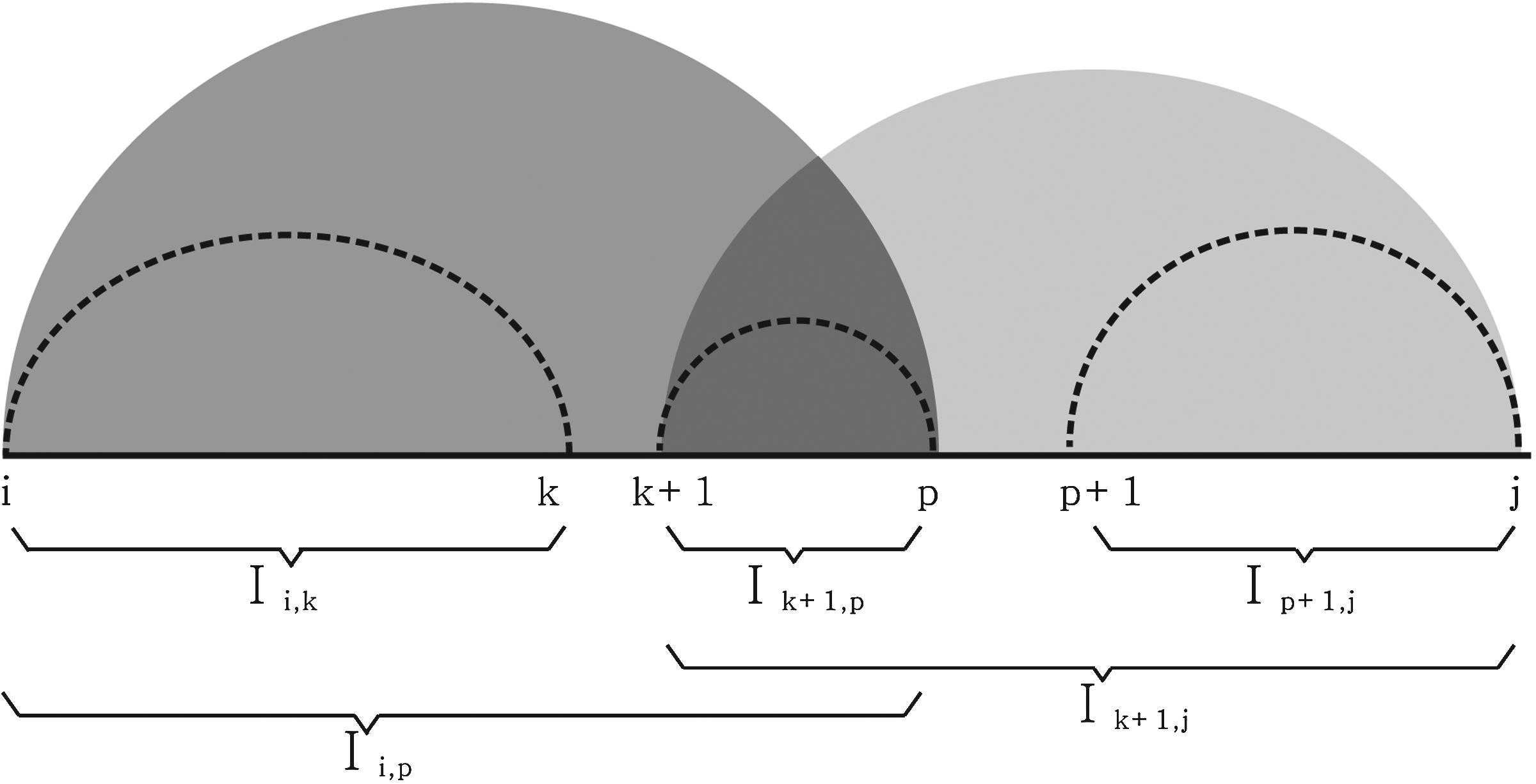
In the context of polynomial-time DP algorithms a particular method, the sparsification, has been devised. Sparsification is tailored to speed up DP-algorithms predicting minimum free energy (mfe)-secondary structures (Wexler et al., 2007; Backofen et al., 2011) by pruning certain computation paths encountered in the DP-recursions (Fig. 2). In the context of the folding of RNA secondary structures, sparsification reduces the DP-recursion paths to be based on so-called candidates. A candidate is in this case an interval, for which the optimal solution cannot be written as a sum of optimal solutions of subintervals. Tracing back these candidates gives rise to irreducible structures, and the crucial observation is here that these irreducibles appear only at a low frequency. This means that only relatively few candidates have to be considered, which in turn implies a significant reduction in time and space complexity.
Sparsification: suppose the optimal solution Ii,j is obtained from the optimal solutions Ii,k, Ik+1,p, and Ip+1,j. Based on the recursions of the secondary structures, Ii,k and Ik+1,p produce an optimal solution of Ii,p. Similarly, Ik+1,p and Ip+1,j produce an optimal solution of Ik+1,j. Now, in order to obtain an optimal solution of Ii,j, it is sufficient to consider either the grouping Ii,p and Ip+1,j or Ii,k and Ik+1,j.
In this paper, we study the effect of the particular choice of energy parameters on sparsification. In other words, we study what happens to RNA structures of a certain energy and quantify the effect of sparsification of their mfe-folding. We shall see that this energy filtration of secondary structures can have a dramatic effect on the structures having significant implication for the effect of sparsification.
The energy parameters are associated with the loops of a secondary structure; they are empirically measured enthalpic and entropic terms that depend on loop sequence, length, and type (Mathews et al., 1999). We shall restrict ourselves to a simplified notion of energy that does not take into account the specifics of nucleotides but only depends on the combinatorial representation of the secondary structure. For instance, the free energy of a hairpin loop H, GH, is given by
\documentclass{aastex}\usepackage{amsbsy}\usepackage{amsfonts}\usepackage{amssymb}\usepackage{bm}\usepackage{mathrsfs}\usepackage{pifont}\usepackage{stmaryrd}\usepackage{textcomp}\usepackage{portland, xspace}\usepackage{amsmath, amsxtra}\pagestyle{empty}\DeclareMathSizes{10}{9}{7}{6}\begin{document}
\begin{align*}G_H = \alpha_1 + \alpha_2 \ell_H + \alpha_3 \quad {
\rm and} \quad Q_H = v^{G_H} , \tag{1.1}\end{align*}
\end{document}
α1 being the penalty for forming H, α2 the penalty for an unpaired base, α3 the score associated with a tetra-loop, ℓH denoting the number of unpaired bases, and QH being the weight of H. The other two loop-types are treated along these lines.
Equipped with this notion of “combinatorial” energy, we study the energy filtration of RNA secondary structures. In light of the above discussion about the candidates and sparsification, we pay particular attention to irreducible RNA secondary structures. One key question here being: Under which conditions does the probability of finding an irreducible minimum-free energy structure tend to zero for larger and larger sequences?
The main results of this paper are as follows. We will show that
• for energy parameters mimicking the established Turner energy model (Mathews et al., 1999), sparsification implies a time and space reduction by a constant factor,
• there exists energy parameters close to those of the Turner energy model (Mathews et al., 1999) for which sparsification implies a linear time reduction,
• the effect of sparsification is closely connected to the distribution of irreducibles within secondary structures. To be precise, we prove that this distribution undergoes a phase transition from a discrete limit law to a central limit law,
• the limit distribution of irreducibles at the phase transition is a Rayleigh law, and a DP-folding in this regimen experiences a linear reduction in space and time.
2. Some Basic Facts
As mentioned above, we present an RNA secondary structure as a diagram by drawing its backbone as a horizontal line containing vertices corresponding to the labels of the nucleotides, and each Watson-Crick base pair as an arc or chord in the upper halfplane. Consequently, the diagram representation ignores the particular type of nucleotides. Any such pair may be inserted in two positions i, j incident to an arc, as long as it is compatible with the Watson-Crick and G-U base paring rules.
The length of one chord (i, j) is ℓ = j − i, and in this article, we only consider RNA secondary structure with chord length ≥4 (Fig. 3). A chord connecting the first and last vertices is called a rainbow, and a RNA secondary structure exhibiting a rainbow is an irreducible RNA secondary structure. This notion of irreducibility comes up naturally when one decomposes a structure by means of cutting the backbone in two positions without breaking any arcs. Let \documentclass{aastex}\usepackage{amsbsy}\usepackage{amsfonts}\usepackage{amssymb}\usepackage{bm}\usepackage{mathrsfs}\usepackage{pifont}\usepackage{stmaryrd}\usepackage{textcomp}\usepackage{portland, xspace}\usepackage{amsmath, amsxtra}\pagestyle{empty}\DeclareMathSizes{10}{9}{7}{6}\begin{document}
$${ \cal s} ( n )$$
\end{document} and \documentclass{aastex}\usepackage{amsbsy}\usepackage{amsfonts}\usepackage{amssymb}\usepackage{bm}\usepackage{mathrsfs}\usepackage{pifont}\usepackage{stmaryrd}\usepackage{textcomp}\usepackage{portland, xspace}\usepackage{amsmath, amsxtra}\pagestyle{empty}\DeclareMathSizes{10}{9}{7}{6}\begin{document}
$${ \cal c} ( n )$$
\end{document} denote the collections of all linear chord diagrams of RNA secondary structures and irreducible secondary structures on n vertices, respectively. Let s(n) and c(n) denote the cardinalities of these sets. Furthermore, setting \documentclass{aastex}\usepackage{amsbsy}\usepackage{amsfonts}\usepackage{amssymb}\usepackage{bm}\usepackage{mathrsfs}\usepackage{pifont}\usepackage{stmaryrd}\usepackage{textcomp}\usepackage{portland, xspace}\usepackage{amsmath, amsxtra}\pagestyle{empty}\DeclareMathSizes{10}{9}{7}{6}\begin{document}
$${ \cal S} = \cup_{n \geq 0} \ { \cal S} ( n )$$
\end{document} and \documentclass{aastex}\usepackage{amsbsy}\usepackage{amsfonts}\usepackage{amssymb}\usepackage{bm}\usepackage{mathrsfs}\usepackage{pifont}\usepackage{stmaryrd}\usepackage{textcomp}\usepackage{portland, xspace}\usepackage{amsmath, amsxtra}\pagestyle{empty}\DeclareMathSizes{10}{9}{7}{6}\begin{document}
$${ \cal C} = \cup_{n \geq 0} \ { \cal C} ( n )$$
\end{document} denote the set of all linear chord diagrams of RNA secondary structures and irreducible secondary structures, let \documentclass{aastex}\usepackage{amsbsy}\usepackage{amsfonts}\usepackage{amssymb}\usepackage{bm}\usepackage{mathrsfs}\usepackage{pifont}\usepackage{stmaryrd}\usepackage{textcomp}\usepackage{portland, xspace}\usepackage{amsmath, amsxtra}\pagestyle{empty}\DeclareMathSizes{10}{9}{7}{6}\begin{document}
$$s \in { \cal S}$$
\end{document} and \documentclass{aastex}\usepackage{amsbsy}\usepackage{amsfonts}\usepackage{amssymb}\usepackage{bm}\usepackage{mathrsfs}\usepackage{pifont}\usepackage{stmaryrd}\usepackage{textcomp}\usepackage{portland, xspace}\usepackage{amsmath, amsxtra}\pagestyle{empty}\DeclareMathSizes{10}{9}{7}{6}\begin{document}
$$c \in { \cal C}$$
\end{document} denote a \documentclass{aastex}\usepackage{amsbsy}\usepackage{amsfonts}\usepackage{amssymb}\usepackage{bm}\usepackage{mathrsfs}\usepackage{pifont}\usepackage{stmaryrd}\usepackage{textcomp}\usepackage{portland, xspace}\usepackage{amsmath, amsxtra}\pagestyle{empty}\DeclareMathSizes{10}{9}{7}{6}\begin{document}
$${ \cal S}$$
\end{document}- or \documentclass{aastex}\usepackage{amsbsy}\usepackage{amsfonts}\usepackage{amssymb}\usepackage{bm}\usepackage{mathrsfs}\usepackage{pifont}\usepackage{stmaryrd}\usepackage{textcomp}\usepackage{portland, xspace}\usepackage{amsmath, amsxtra}\pagestyle{empty}\DeclareMathSizes{10}{9}{7}{6}\begin{document}
$${ \cal C}$$
\end{document}-structure.
A diagram representation of secondary structure with ≥4.
Let \documentclass{aastex}\usepackage{amsbsy}\usepackage{amsfonts}\usepackage{amssymb}\usepackage{bm}\usepackage{mathrsfs}\usepackage{pifont}\usepackage{stmaryrd}\usepackage{textcomp}\usepackage{portland, xspace}\usepackage{amsmath, amsxtra}\pagestyle{empty}\DeclareMathSizes{10}{9}{7}{6}\begin{document}
$${ \cal S} ( n , j , i ) \supseteq \ { \cal C} ( n , j , i )$$
\end{document} denote the collections of RNA secondary structures and irreducible RNA secondary structures on n ≥ 0 vertices having length n, energy j, and weight i, then
\documentclass{aastex}\usepackage{amsbsy}\usepackage{amsfonts}\usepackage{amssymb}\usepackage{bm}\usepackage{mathrsfs}\usepackage{pifont}\usepackage{stmaryrd}\usepackage{textcomp}\usepackage{portland, xspace}\usepackage{amsmath, amsxtra}\pagestyle{empty}\DeclareMathSizes{10}{9}{7}{6}\begin{document}
\begin{align*} { \bf S} ( z , v , p ) = \sum_{n \geq
0} \sum_{j} \sum_{i \geq 0} { \bf s} ( n , j , i ) z^n v^j p^i
\tag {2.1}\end{align*}
\end{document}\documentclass{aastex}\usepackage{amsbsy}\usepackage{amsfonts}\usepackage{amssymb}\usepackage{bm}\usepackage{mathrsfs}\usepackage{pifont}\usepackage{stmaryrd}\usepackage{textcomp}\usepackage{portland, xspace}\usepackage{amsmath, amsxtra}\pagestyle{empty}\DeclareMathSizes{10}{9}{7}{6}\begin{document}
\begin{align*} { \bf C} ( z , v , p ) = \sum_{n \geq 0} \sum_{j}
\sum_{i \geq 0} { \bf c} ( n , j , i ) z^n v^j p^i.\end{align*}
\end{document}
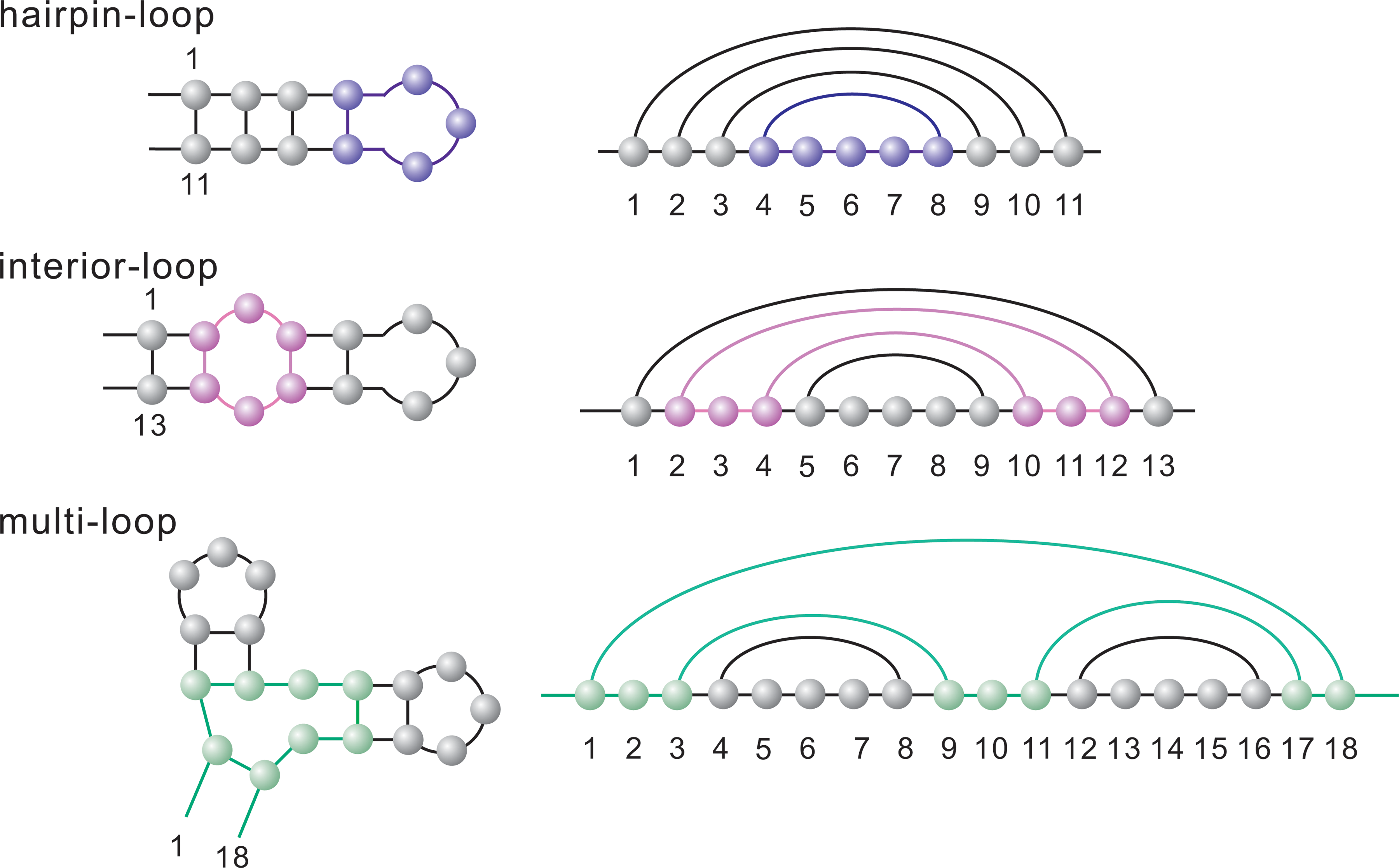
Thermodynamic models for nucleic acid secondary structure are based on a decomposition of the base-pairing diagram of structures into distinct loops that are associated with empirically measured enthalpic and entropic terms that depend on loop sequence, length, and type (SantaLucia, 1996; Mathews et al., 1999). To obtain a better idea about these loops, we give the diagram representations of three types of Loops L:
• a Hairpin-loop (H) consists of a chord (i, j) with a sequence of unpaired bases [i + 1, j − 1]. In particular, we have the restriction j − i ≥ 4; if j − i = 4 (tetra-loop);
• an interior-loop (I) consists of two base pairs (i, j) and (i1, j1) and three sequence of unpaired bases [i + 1, i1 − 1], [j1 + 1, j − 1] and [i1 − 1,j1 − 1]. The case of i + 1 = i1 − 1 and i1 − 1 = j1 − 1 is referred to as helix;
with sequences of unpaired bases [jk-1 + 1, ik − 1], for k ≥ 2 (Fig. 4).
This figure illustrates a hairpin-loop (H), interior-loop (I), and multi-loop (M).
The free energy Gs of a secondary structure s is the sum of the energies of its constituent Loops L (Mathews et al., 1999). Thus the total free energy Gs is given by \documentclass{aastex}\usepackage{amsbsy}\usepackage{amsfonts}\usepackage{amssymb}\usepackage{bm}\usepackage{mathrsfs}\usepackage{pifont}\usepackage{stmaryrd}\usepackage{textcomp}\usepackage{portland, xspace}\usepackage{amsmath, amsxtra}\pagestyle{empty}\DeclareMathSizes{10}{9}{7}{6}\begin{document}
$$G_s = \sum \nolimits_{L \in s} G_L$$
\end{document}. This notion of energy allows one to compute, by means of dynamic programming (Zuker and Stiegler, 1981, Hofacker et al., 1994) the minimum free energy configurations as well as the partition function (McCaskill, 1990) as a weighted sum \documentclass{aastex}\usepackage{amsbsy}\usepackage{amsfonts}\usepackage{amssymb}\usepackage{bm}\usepackage{mathrsfs}\usepackage{pifont}\usepackage{stmaryrd}\usepackage{textcomp}\usepackage{portland, xspace}\usepackage{amsmath, amsxtra}\pagestyle{empty}\DeclareMathSizes{10}{9}{7}{6}\begin{document}
$$Q = \sum \nolimits_{s \in { \cal S}} e^{G_s / RT}$$
\end{document}, where R is the universal gas constant, T is the temperature, and \documentclass{aastex}\usepackage{amsbsy}\usepackage{amsfonts}\usepackage{amssymb}\usepackage{bm}\usepackage{mathrsfs}\usepackage{pifont}\usepackage{stmaryrd}\usepackage{textcomp}\usepackage{portland, xspace}\usepackage{amsmath, amsxtra}\pagestyle{empty}\DeclareMathSizes{10}{9}{7}{6}\begin{document}
$$e^{G_s / RT}$$
\end{document} is the weight of sampling a secondary structure s with free energy Gs.
In the following, we consider a notion of energy that does not take into account the specifics of nucleotides and only depends on the combinatorial representation of the secondary structure. Our energy model is based on seven parameters \documentclass{aastex}\usepackage{amsbsy}\usepackage{amsfonts}\usepackage{amssymb}\usepackage{bm}\usepackage{mathrsfs}\usepackage{pifont}\usepackage{stmaryrd}\usepackage{textcomp}\usepackage{portland, xspace}\usepackage{amsmath, amsxtra}\pagestyle{empty}\DeclareMathSizes{10}{9}{7}{6}\begin{document}
$${\cal P} = \{\alpha_1, \alpha_2, \alpha_3, \beta_1, \beta_2, \gamma_1, \gamma_2 \}$$
\end{document} defined as follows:
where GH is the free energy of H, α1 is the penalty for forming H, α2 is the penalty for an unpaired base, and α3 is a score associated to a tetra-loop. Furthermore, ℓH denotes the number of unpaired bases, and QH is the weight of H.
where GI is free energy of I, β1 is a favorable bonus of a helix, and β2 is the penalty of an unpaired base of I. Furthermore, ℓI denotes the total number of unpaired bases of I, and QI is the weight of I.
• Multi-loop M:
\documentclass{aastex}\usepackage{amsbsy}\usepackage{amsfonts}\usepackage{amssymb}\usepackage{bm}\usepackage{mathrsfs}\usepackage{pifont}\usepackage{stmaryrd}\usepackage{textcomp}\usepackage{portland, xspace}\usepackage{amsmath, amsxtra}\pagestyle{empty}\DeclareMathSizes{10}{9}{7}{6}\begin{document}
\begin{align*}G_{M} \sim \gamma_1 + B \gamma_2 + U \times 0 \quad
and \quad Q_{M} = v^{G_{M}} \tag{2.4}\end{align*}
\end{document}
GM is the free energy of M, γ1 is the penalty for the formation of a multi-loop, B is the number of base pairs defining the multi-loop (including the closing pair i · j), and U is the number of unpaired bases in the multi-loop; γ2 is the penalty for the base pair defining the multi-loop, and QM is the weight of one M.
This energy model induces the partition function
\documentclass{aastex}\usepackage{amsbsy}\usepackage{amsfonts}\usepackage{amssymb}\usepackage{bm}\usepackage{mathrsfs}\usepackage{pifont}\usepackage{stmaryrd}\usepackage{textcomp}\usepackage{portland, xspace}\usepackage{amsmath, amsxtra}\pagestyle{empty}\DeclareMathSizes{10}{9}{7}{6}\begin{document}
\begin{align*}Q = \sum_{s \in \ { \cal S} ( n ) } v^{G_s} , \tag{2.5}\end{align*}
\end{document}
where \documentclass{aastex}\usepackage{amsbsy}\usepackage{amsfonts}\usepackage{amssymb}\usepackage{bm}\usepackage{mathrsfs}\usepackage{pifont}\usepackage{stmaryrd}\usepackage{textcomp}\usepackage{portland, xspace}\usepackage{amsmath, amsxtra}\pagestyle{empty}\DeclareMathSizes{10}{9}{7}{6}\begin{document}
$$v^{G_s}$$
\end{document} is the weight for sampling a secondary structure with free energy Gs.
3. Energy Filtration
Theorem 1.The trivariate generating functionC(z, v, p) counting RNA secondary structures having length n, energy i, and j arcs, satisfies the following recursion:\documentclass{aastex}\usepackage{amsbsy}\usepackage{amsfonts}\usepackage{amssymb}\usepackage{bm}\usepackage{mathrsfs}\usepackage{pifont}\usepackage{stmaryrd}\usepackage{textcomp}\usepackage{portland, xspace}\usepackage{amsmath, amsxtra}\pagestyle{empty}\DeclareMathSizes{10}{9}{7}{6}\begin{document}
\begin{align*} { \bf C } ( z , v , p ) & = p v^ { \alpha_1 } z^2
\bigg( \frac { ( zv^ { \alpha_2 } ) ^3 } { 1 - zv^ { \alpha_2
} } + z^4v^ { \alpha_3 } - z^4v^ { 4 \alpha_2 } \bigg) \\
&\quad+ p \frac { z^2v^ { \beta_1 } } { ( 1 - zv^ { \beta_2 } )
^2 } { \bf C } ( z , v , p ) + p \frac { v^ { \gamma_1 } ( z^2v^ {
\gamma_2 } ) ( { \bf C } ( z , v , p ) v^ { \gamma_2 } ) ^2 } { (
( 1 - z ) ^3 - { \bf C } ( z , v , p ) v^ { \gamma_2 } ( 1 - z )
^2 ) } . \tag{3.1} \end{align*}
\end{document}
The proof is a straightforward exercise in symbolic methods and will consequently be omitted.
We shall pass from the trivariate generating function to univariate ones by specifying the indeterminants v and p as follows: Since there are a total of four nucleotides A, G, U, and C and only six base pairs, namely GC, CG, AU, UA, UG, and GU, we set p = 6/16. This choice reflects the probability of randomly forming a (valid) base pair. We proceed similarly for the indeterminant v setting \documentclass{aastex}\usepackage{amsbsy}\usepackage{amsfonts}\usepackage{amssymb}\usepackage{bm}\usepackage{mathrsfs}\usepackage{pifont}\usepackage{stmaryrd}\usepackage{textcomp}\usepackage{portland, xspace}\usepackage{amsmath, amsxtra}\pagestyle{empty}\DeclareMathSizes{10}{9}{7}{6}\begin{document}
$$v = e^ { \frac { 1 } { RT } } \approx 1.843868184$$
\end{document}.
These two choices induce the univariate generating functions \documentclass{aastex}\usepackage{amsbsy}\usepackage{amsfonts}\usepackage{amssymb}\usepackage{bm}\usepackage{mathrsfs}\usepackage{pifont}\usepackage{stmaryrd}\usepackage{textcomp}\usepackage{portland, xspace}\usepackage{amsmath, amsxtra}\pagestyle{empty}\DeclareMathSizes{10}{9}{7}{6}\begin{document}
$${ \bf C}^{*} ( z ) = \sum \nolimits_{n \geq 0} { \bf c}^{*} ( n ) z^n$$
\end{document}, \documentclass{aastex}\usepackage{amsbsy}\usepackage{amsfonts}\usepackage{amssymb}\usepackage{bm}\usepackage{mathrsfs}\usepackage{pifont}\usepackage{stmaryrd}\usepackage{textcomp}\usepackage{portland, xspace}\usepackage{amsmath, amsxtra}\pagestyle{empty}\DeclareMathSizes{10}{9}{7}{6}\begin{document}
$${ \bf S}^{*} ( z ) = \sum \nolimits_{n \geq 0} { \bf s}^{*} ( n ) z^n$$
\end{document}, and the sets of \documentclass{aastex}\usepackage{amsbsy}\usepackage{amsfonts}\usepackage{amssymb}\usepackage{bm}\usepackage{mathrsfs}\usepackage{pifont}\usepackage{stmaryrd}\usepackage{textcomp}\usepackage{portland, xspace}\usepackage{amsmath, amsxtra}\pagestyle{empty}\DeclareMathSizes{10}{9}{7}{6}\begin{document}
$${ \cal S}^*$$
\end{document} and \documentclass{aastex}\usepackage{amsbsy}\usepackage{amsfonts}\usepackage{amssymb}\usepackage{bm}\usepackage{mathrsfs}\usepackage{pifont}\usepackage{stmaryrd}\usepackage{textcomp}\usepackage{portland, xspace}\usepackage{amsmath, amsxtra}\pagestyle{empty}\DeclareMathSizes{10}{9}{7}{6}\begin{document}
$${ \cal C}^*$$
\end{document}, which are weighted set of \documentclass{aastex}\usepackage{amsbsy}\usepackage{amsfonts}\usepackage{amssymb}\usepackage{bm}\usepackage{mathrsfs}\usepackage{pifont}\usepackage{stmaryrd}\usepackage{textcomp}\usepackage{portland, xspace}\usepackage{amsmath, amsxtra}\pagestyle{empty}\DeclareMathSizes{10}{9}{7}{6}\begin{document}
$${ \cal S}$$
\end{document} and \documentclass{aastex}\usepackage{amsbsy}\usepackage{amsfonts}\usepackage{amssymb}\usepackage{bm}\usepackage{mathrsfs}\usepackage{pifont}\usepackage{stmaryrd}\usepackage{textcomp}\usepackage{portland, xspace}\usepackage{amsmath, amsxtra}\pagestyle{empty}\DeclareMathSizes{10}{9}{7}{6}\begin{document}
$${ \cal C}$$
\end{document}, separately. Furthermore, c*(n) or s*(n) denotes the summation of energy weight of all the \documentclass{aastex}\usepackage{amsbsy}\usepackage{amsfonts}\usepackage{amssymb}\usepackage{bm}\usepackage{mathrsfs}\usepackage{pifont}\usepackage{stmaryrd}\usepackage{textcomp}\usepackage{portland, xspace}\usepackage{amsmath, amsxtra}\pagestyle{empty}\DeclareMathSizes{10}{9}{7}{6}\begin{document}
$${ \cal C}^*$$
\end{document}-structures or \documentclass{aastex}\usepackage{amsbsy}\usepackage{amsfonts}\usepackage{amssymb}\usepackage{bm}\usepackage{mathrsfs}\usepackage{pifont}\usepackage{stmaryrd}\usepackage{textcomp}\usepackage{portland, xspace}\usepackage{amsmath, amsxtra}\pagestyle{empty}\DeclareMathSizes{10}{9}{7}{6}\begin{document}
$${ \cal S}^*$$
\end{document}-structures with length n.
We have c*(n) = 0, s*(n) = 0, for \documentclass{aastex}\usepackage{amsbsy}\usepackage{amsfonts}\usepackage{amssymb}\usepackage{bm}\usepackage{mathrsfs}\usepackage{pifont}\usepackage{stmaryrd}\usepackage{textcomp}\usepackage{portland, xspace}\usepackage{amsmath, amsxtra}\pagestyle{empty}\DeclareMathSizes{10}{9}{7}{6}\begin{document}
$$n = 0 , \ldots , 4$$
\end{document}; and c*(n) > 0, s*(n) > 0, for n ≥ 5 (see Claim 0 of Lemma 2).
Symbolic methods immediately imply
Theorem 2.The bivariate generating functionS*(z) is given by:\documentclass{aastex}\usepackage{amsbsy}\usepackage{amsfonts}\usepackage{amssymb}\usepackage{bm}\usepackage{mathrsfs}\usepackage{pifont}\usepackage{stmaryrd}\usepackage{textcomp}\usepackage{portland, xspace}\usepackage{amsmath, amsxtra}\pagestyle{empty}\DeclareMathSizes{10}{9}{7}{6}\begin{document}
\begin{align*}{ \bf S}^* ( z ) = 1 / ( 1 - ( z + { \bf C}^* ( z )
) ) \tag{3.2}\end{align*}
\end{document}
and furthermore,S*(z, t) is\documentclass{aastex}\usepackage{amsbsy}\usepackage{amsfonts}\usepackage{amssymb}\usepackage{bm}\usepackage{mathrsfs}\usepackage{pifont}\usepackage{stmaryrd}\usepackage{textcomp}\usepackage{portland, xspace}\usepackage{amsmath, amsxtra}\pagestyle{empty}\DeclareMathSizes{10}{9}{7}{6}\begin{document}
\begin{align*}{ \bf S}^* ( z , t ) = 1 / ( 1 - ( z + t { \bf C}^*
( z ) ) ) . \tag{3.3}\end{align*}
\end{document}
The key for the following analysis is to study the dominant singularities of C*(z) and S*(z). It is their relative location and behavior that is responsible for the observed limit distributions as well as the effect of sparsification.
We begin our analysis by making the following observations. Theorem 1 implies
\documentclass{aastex}\usepackage{amsbsy}\usepackage{amsfonts}\usepackage{amssymb}\usepackage{bm}\usepackage{mathrsfs}\usepackage{pifont}\usepackage{stmaryrd}\usepackage{textcomp}\usepackage{portland, xspace}\usepackage{amsmath, amsxtra}\pagestyle{empty}\DeclareMathSizes{10}{9}{7}{6}\begin{document}
\begin{align*}w^*_2 ( z ) { \bf C}^{*} ( z ) ^2 + w^{*}_1 ( z ) {
\bf C}^{*} ( z ) + w^{*}_0 ( z ) = 0 , \tag{3.4}\end{align*}
\end{document}
We observe that only one solution of Equation (3.4) has the property c*(n) > 0, namely
\documentclass{aastex}\usepackage{amsbsy}\usepackage{amsfonts}\usepackage{amssymb}\usepackage{bm}\usepackage{mathrsfs}\usepackage{pifont}\usepackage{stmaryrd}\usepackage{textcomp}\usepackage{portland, xspace}\usepackage{amsmath, amsxtra}\pagestyle{empty}\DeclareMathSizes{10}{9}{7}{6}\begin{document}
\begin{align*}{ \bf C}^* ( z ) = N^* ( z ) / D^* ( z ) , \tag{3.5}\end{align*}
\end{document}
where \documentclass{aastex}\usepackage{amsbsy}\usepackage{amsfonts}\usepackage{amssymb}\usepackage{bm}\usepackage{mathrsfs}\usepackage{pifont}\usepackage{stmaryrd}\usepackage{textcomp}\usepackage{portland, xspace}\usepackage{amsmath, amsxtra}\pagestyle{empty}\DeclareMathSizes{10}{9}{7}{6}\begin{document}
$$N^{*} ( z ) = - w_1^{*} ( z ) + \sqrt{w^{*}_1 ( z ) ^2 - 4w_2^{*} ( z ) w_0^{*} ( z ) }$$
\end{document} and \documentclass{aastex}\usepackage{amsbsy}\usepackage{amsfonts}\usepackage{amssymb}\usepackage{bm}\usepackage{mathrsfs}\usepackage{pifont}\usepackage{stmaryrd}\usepackage{textcomp}\usepackage{portland, xspace}\usepackage{amsmath, amsxtra}\pagestyle{empty}\DeclareMathSizes{10}{9}{7}{6}\begin{document}
$$D^* ( z ) = 2w_2^* ( z )$$
\end{document}.
Let \documentclass{aastex}\usepackage{amsbsy}\usepackage{amsfonts}\usepackage{amssymb}\usepackage{bm}\usepackage{mathrsfs}\usepackage{pifont}\usepackage{stmaryrd}\usepackage{textcomp}\usepackage{portland, xspace}\usepackage{amsmath, amsxtra}\pagestyle{empty}\DeclareMathSizes{10}{9}{7}{6}\begin{document}
$$\rho_{c^{*}}$$
\end{document} denote the radius of convergence of C*(z) and \documentclass{aastex}\usepackage{amsbsy}\usepackage{amsfonts}\usepackage{amssymb}\usepackage{bm}\usepackage{mathrsfs}\usepackage{pifont}\usepackage{stmaryrd}\usepackage{textcomp}\usepackage{portland, xspace}\usepackage{amsmath, amsxtra}\pagestyle{empty}\DeclareMathSizes{10}{9}{7}{6}\begin{document}
$$\rho_{s^{*}}$$
\end{document} denote the radius of convergence of S*(z). Then, clearly, \documentclass{aastex}\usepackage{amsbsy}\usepackage{amsfonts}\usepackage{amssymb}\usepackage{bm}\usepackage{mathrsfs}\usepackage{pifont}\usepackage{stmaryrd}\usepackage{textcomp}\usepackage{portland, xspace}\usepackage{amsmath, amsxtra}\pagestyle{empty}\DeclareMathSizes{10}{9}{7}{6}\begin{document}
$$0 < \rho_{c^{*}} < 1$$
\end{document} and in view of \documentclass{aastex}\usepackage{amsbsy}\usepackage{amsfonts}\usepackage{amssymb}\usepackage{bm}\usepackage{mathrsfs}\usepackage{pifont}\usepackage{stmaryrd}\usepackage{textcomp}\usepackage{portland, xspace}\usepackage{amsmath, amsxtra}\pagestyle{empty}\DeclareMathSizes{10}{9}{7}{6}\begin{document}
$${ \cal C}^* \subset { \cal S}^*$$
\end{document}, we have \documentclass{aastex}\usepackage{amsbsy}\usepackage{amsfonts}\usepackage{amssymb}\usepackage{bm}\usepackage{mathrsfs}\usepackage{pifont}\usepackage{stmaryrd}\usepackage{textcomp}\usepackage{portland, xspace}\usepackage{amsmath, amsxtra}\pagestyle{empty}\DeclareMathSizes{10}{9}{7}{6}\begin{document}
$$0 < \rho_{s^{*}} \leq \rho_{c^{*}} < 1$$
\end{document}.
• Furthermore, let ρr denote the minimum positive real root of odd order of the discriminant
\documentclass{aastex}\usepackage{amsbsy}\usepackage{amsfonts}\usepackage{amssymb}\usepackage{bm}\usepackage{mathrsfs}\usepackage{pifont}\usepackage{stmaryrd}\usepackage{textcomp}\usepackage{portland, xspace}\usepackage{amsmath, amsxtra}\pagestyle{empty}\DeclareMathSizes{10}{9}{7}{6}\begin{document}
\begin{align*}w^{*}_1 ( z ) ^2 - 4w^{*}_2 ( z ) w^{*}_0 ( z ) = 0.\end{align*}
\end{document}
• Let ρd and ρp denote the minimum positive real roots of the equations
\documentclass{aastex}\usepackage{amsbsy}\usepackage{amsfonts}\usepackage{amssymb}\usepackage{bm}\usepackage{mathrsfs}\usepackage{pifont}\usepackage{stmaryrd}\usepackage{textcomp}\usepackage{portland, xspace}\usepackage{amsmath, amsxtra}\pagestyle{empty}\DeclareMathSizes{10}{9}{7}{6}\begin{document}
\begin{align*}w_2^* ( z ) = 0 \quad { \rm and} \quad 1 - ( z + {
\bf C}^* ( z ) ) = 0.\end{align*}
\end{document}
Theorem 3.(Pringsheim'stheorem)(Titchmarsh, 1939): If f (z) is representable at the origin by a series expansion that has non-negative coefficients and radius of convergence r, then the point z = r is a dominant singularity of f (z).
Lemma 1.For the positive dominant real singularities ofC*(z) andS*(z),\documentclass{aastex}\usepackage{amsbsy}\usepackage{amsfonts}\usepackage{amssymb}\usepackage{bm}\usepackage{mathrsfs}\usepackage{pifont}\usepackage{stmaryrd}\usepackage{textcomp}\usepackage{portland, xspace}\usepackage{amsmath, amsxtra}\pagestyle{empty}\DeclareMathSizes{10}{9}{7}{6}\begin{document}
$$\rho_{c^*}$$
\end{document}and\documentclass{aastex}\usepackage{amsbsy}\usepackage{amsfonts}\usepackage{amssymb}\usepackage{bm}\usepackage{mathrsfs}\usepackage{pifont}\usepackage{stmaryrd}\usepackage{textcomp}\usepackage{portland, xspace}\usepackage{amsmath, amsxtra}\pagestyle{empty}\DeclareMathSizes{10}{9}{7}{6}\begin{document}
$$\rho_{s^*}$$
\end{document}, we distinguish the following three cases:
Proof. According to Theorem 3, we have \documentclass{aastex}\usepackage{amsbsy}\usepackage{amsfonts}\usepackage{amssymb}\usepackage{bm}\usepackage{mathrsfs}\usepackage{pifont}\usepackage{stmaryrd}\usepackage{textcomp}\usepackage{portland, xspace}\usepackage{amsmath, amsxtra}\pagestyle{empty}\DeclareMathSizes{10}{9}{7}{6}\begin{document}
$$\rho_{c^*} = \min \{ \rho_r , \rho_d \} $$
\end{document}.
Claim 0: We have ρd ≠ ρr.
To prove Claim 0, we begin by observing that \documentclass{aastex}\usepackage{amsbsy}\usepackage{amsfonts}\usepackage{amssymb}\usepackage{bm}\usepackage{mathrsfs}\usepackage{pifont}\usepackage{stmaryrd}\usepackage{textcomp}\usepackage{portland, xspace}\usepackage{amsmath, amsxtra}\pagestyle{empty}\DeclareMathSizes{10}{9}{7}{6}\begin{document}
$$v^{4 \alpha_2} - v^{ \alpha_3} < 0$$
\end{document}, since α2 < 0, α3 > 0 and v > 1, then for arbitrary real z, 0 < z < 1,
\documentclass{aastex}\usepackage{amsbsy}\usepackage{amsfonts}\usepackage{amssymb}\usepackage{bm}\usepackage{mathrsfs}\usepackage{pifont}\usepackage{stmaryrd}\usepackage{textcomp}\usepackage{portland, xspace}\usepackage{amsmath, amsxtra}\pagestyle{empty}\DeclareMathSizes{10}{9}{7}{6}\begin{document}
\begin{align*}w^{*}_0 ( z ) = 6v^{ \alpha_1}z^5 \underbrace{ ( 1
- z ) ^3 ( 1 - z v^{ \beta_2} ) ^2}_{ > 0} ( v^{3 \alpha_2} - z
\underbrace{ ( v^{4 \alpha_2} - v^{ \alpha_3} ) }_{ < 0}
\underbrace{ ( 1 - z v^{ \alpha_2} ) }_{ > 0} ) > 0.\end{align*}
\end{document}
and, consequently, \documentclass{aastex}\usepackage{amsbsy}\usepackage{amsfonts}\usepackage{amssymb}\usepackage{bm}\usepackage{mathrsfs}\usepackage{pifont}\usepackage{stmaryrd}\usepackage{textcomp}\usepackage{portland, xspace}\usepackage{amsmath, amsxtra}\pagestyle{empty}\DeclareMathSizes{10}{9}{7}{6}\begin{document}
$$w_1^* ( \rho_d ) = 0$$
\end{document}. But in this case Equation (3.4) implies \documentclass{aastex}\usepackage{amsbsy}\usepackage{amsfonts}\usepackage{amssymb}\usepackage{bm}\usepackage{mathrsfs}\usepackage{pifont}\usepackage{stmaryrd}\usepackage{textcomp}\usepackage{portland, xspace}\usepackage{amsmath, amsxtra}\pagestyle{empty}\DeclareMathSizes{10}{9}{7}{6}\begin{document}
$$w_0^* ( \rho_d ) = 0$$
\end{document}, which conflicts with \documentclass{aastex}\usepackage{amsbsy}\usepackage{amsfonts}\usepackage{amssymb}\usepackage{bm}\usepackage{mathrsfs}\usepackage{pifont}\usepackage{stmaryrd}\usepackage{textcomp}\usepackage{portland, xspace}\usepackage{amsmath, amsxtra}\pagestyle{empty}\DeclareMathSizes{10}{9}{7}{6}\begin{document}
$$w_0^* ( \rho_d ) > 0$$
\end{document} and Claim 0 is proved.
First, we discuss the case ρd < ρr.
Claim 1: ρd is a removable singularity of C*(z).
To prove Claim 1. Suppose first N*(ρd) ≠ 0, since D*(ρd) = 0, thus limz→ρdC*(z) = ∞ , so ρd is accordingly a pole of C*(z).
In view of
\documentclass{aastex}\usepackage{amsbsy}\usepackage{amsfonts}\usepackage{amssymb}\usepackage{bm}\usepackage{mathrsfs}\usepackage{pifont}\usepackage{stmaryrd}\usepackage{textcomp}\usepackage{portland, xspace}\usepackage{amsmath, amsxtra}\pagestyle{empty}\DeclareMathSizes{10}{9}{7}{6}\begin{document}
\begin{align*}{ \bf S}^{*} ( z ) ^{ - 1} = 1 - \left( z + N^{*} (
\rho_{d} ) / D^{*} ( \rho_{d} ) \right) ,\end{align*}
\end{document}
we have limz→ρdS*(z) = 0, this is impossible, since \documentclass{aastex}\usepackage{amsbsy}\usepackage{amsfonts}\usepackage{amssymb}\usepackage{bm}\usepackage{mathrsfs}\usepackage{pifont}\usepackage{stmaryrd}\usepackage{textcomp}\usepackage{portland, xspace}\usepackage{amsmath, amsxtra}\pagestyle{empty}\DeclareMathSizes{10}{9}{7}{6}\begin{document}
$${ \bf S}^{*} ( z ) = \sum \nolimits_{n \geq 0} { \bf s}^{*} ( n ) z^n$$
\end{document}, the only value of ρd to make limz→ρdS*(z) = 0 is ρd = 0.
which implies that ρd is a removable singularity, whence Claim 1.
Claim 2:\documentclass{aastex}\usepackage{amsbsy}\usepackage{amsfonts}\usepackage{amssymb}\usepackage{bm}\usepackage{mathrsfs}\usepackage{pifont}\usepackage{stmaryrd}\usepackage{textcomp}\usepackage{portland, xspace}\usepackage{amsmath, amsxtra}\pagestyle{empty}\DeclareMathSizes{10}{9}{7}{6}\begin{document}
$$z = \rho_{d} e^{i \theta}$$
\end{document}, where 0 < θ < 2π, is not a dominant singularity of C*(z). To prove Claim 2 we assume a contrario that \documentclass{aastex}\usepackage{amsbsy}\usepackage{amsfonts}\usepackage{amssymb}\usepackage{bm}\usepackage{mathrsfs}\usepackage{pifont}\usepackage{stmaryrd}\usepackage{textcomp}\usepackage{portland, xspace}\usepackage{amsmath, amsxtra}\pagestyle{empty}\DeclareMathSizes{10}{9}{7}{6}\begin{document}
$$z = \rho_{d} e^{i \theta}$$
\end{document}, 0 < θ < 2π is a dominant singularity of C*(z). Then the convergence radius of C*(z) is ρd and Theorem 3 implies that ρd is also a dominant singularity of C*(z), which contradicts Claim 1, where we showed that ρd is a removable singularity.
Therefore, in case of ρd < ρr, \documentclass{aastex}\usepackage{amsbsy}\usepackage{amsfonts}\usepackage{amssymb}\usepackage{bm}\usepackage{mathrsfs}\usepackage{pifont}\usepackage{stmaryrd}\usepackage{textcomp}\usepackage{portland, xspace}\usepackage{amsmath, amsxtra}\pagestyle{empty}\DeclareMathSizes{10}{9}{7}{6}\begin{document}
$$\rho_{c^*} \neq \rho_d$$
\end{document}. Consequently, Claim 1 and Claim 2 imply \documentclass{aastex}\usepackage{amsbsy}\usepackage{amsfonts}\usepackage{amssymb}\usepackage{bm}\usepackage{mathrsfs}\usepackage{pifont}\usepackage{stmaryrd}\usepackage{textcomp}\usepackage{portland, xspace}\usepackage{amsmath, amsxtra}\pagestyle{empty}\DeclareMathSizes{10}{9}{7}{6}\begin{document}
$$\rho_{c^*} = \rho_{r}$$
\end{document}.
We thus have the following two scenarios for \documentclass{aastex}\usepackage{amsbsy}\usepackage{amsfonts}\usepackage{amssymb}\usepackage{bm}\usepackage{mathrsfs}\usepackage{pifont}\usepackage{stmaryrd}\usepackage{textcomp}\usepackage{portland, xspace}\usepackage{amsmath, amsxtra}\pagestyle{empty}\DeclareMathSizes{10}{9}{7}{6}\begin{document}
$$\rho_{s^*}$$
\end{document}:
\documentclass{aastex}\usepackage{amsbsy}\usepackage{amsfonts}\usepackage{amssymb}\usepackage{bm}\usepackage{mathrsfs}\usepackage{pifont}\usepackage{stmaryrd}\usepackage{textcomp}\usepackage{portland, xspace}\usepackage{amsmath, amsxtra}\pagestyle{empty}\DeclareMathSizes{10}{9}{7}{6}\begin{document}
\begin{align*}\rho_{s^*} = \begin{cases} \rho_{r} \quad { \rm
for} \quad \rho_{r} < \rho_{p} \\ \rho_{p} \quad { \rm for} \quad
\rho_{p} \le \rho_{r} , \end{cases} \tag{3.6}\end{align*}
\end{document}
It is clear that there always exists some irreducible secondary structure of length n ≥ 5. The coefficients of C*(z) are weighted sums of these structures, and the weights are, by construction, always strictly positive. Therefore, \documentclass{aastex}\usepackage{amsbsy}\usepackage{amsfonts}\usepackage{amssymb}\usepackage{bm}\usepackage{mathrsfs}\usepackage{pifont}\usepackage{stmaryrd}\usepackage{textcomp}\usepackage{portland, xspace}\usepackage{amsmath, amsxtra}\pagestyle{empty}\DeclareMathSizes{10}{9}{7}{6}\begin{document}
$${ \bf C}^{*} ( z ) = \sum \nolimits_{n \geq 0} { \bf c}^{*} ( n ) z^n$$
\end{document} has for n ≥ 5 always strictly positive coefficients, i.e., c*(n) > 0. Hence, there exist three indices i < j < k such that c*(i)c*(j)c*(k) ≠ 0 and gcd(j − i, k − i) = 1, therefore, C*(z) is aperiodic and Claim 0 is proved.
In view of Equation (3.1), we compute
\documentclass{aastex}\usepackage{amsbsy}\usepackage{amsfonts}\usepackage{amssymb}\usepackage{bm}\usepackage{mathrsfs}\usepackage{pifont}\usepackage{stmaryrd}\usepackage{textcomp}\usepackage{portland, xspace}\usepackage{amsmath, amsxtra}\pagestyle{empty}\DeclareMathSizes{10}{9}{7}{6}\begin{document}
\begin{align*} { \bf C} ( z , v , p ) = & pv^{ \alpha_1}z^2 \ (
zv^{ \alpha_2} ) ^3 \sum_{i \geq 0 } ( zv^{ \alpha_2} ) ^i + (
v^{ \alpha_3} - v^{4 \alpha_2} ) z^4 + pz^2v^{ \beta_1}{ \bf C} (
z , v , p ) \left( \sum_{j \geq 0} ( zv^{ \beta_2} ) ^j \right) ^2
\\ & + pv^{ \gamma_1} ( z^2v^{ \gamma_2} ) ( { \bf C} ( z , v
, p ) v^{ \gamma_2} ) ^2 \left( \sum_{k \geq 0} z^k \right)
\sum_{l \geq 0} \left( { \bf C} ( z , v , p ) v^{ \gamma_2}
\sum_{t \geq 0} z^t \right) ^{l}. \tag{3.7} \end{align*}
\end{document}
Setting p = 6/16, \documentclass{aastex}\usepackage{amsbsy}\usepackage{amsfonts}\usepackage{amssymb}\usepackage{bm}\usepackage{mathrsfs}\usepackage{pifont}\usepackage{stmaryrd}\usepackage{textcomp}\usepackage{portland, xspace}\usepackage{amsmath, amsxtra}\pagestyle{empty}\DeclareMathSizes{10}{9}{7}{6}\begin{document}
$$v = e^ { \frac { 1 } { RT } } $$
\end{document} and w = C*(z) = ∑n≥0c*(n)zn, we obtain a power series equation
\documentclass{aastex}\usepackage{amsbsy}\usepackage{amsfonts}\usepackage{amssymb}\usepackage{bm}\usepackage{mathrsfs}\usepackage{pifont}\usepackage{stmaryrd}\usepackage{textcomp}\usepackage{portland, xspace}\usepackage{amsmath, amsxtra}\pagestyle{empty}\DeclareMathSizes{10}{9}{7}{6}\begin{document}
\begin{align*}w = G ( z , w ) , \tag{3.8}\end{align*}
\end{document}
where G(z, w) = ∑m,n>0gm,nzmwn and gm,n ≥ 0. Indeed, since α3 > 0 and α2 < 0, we have \documentclass{aastex}\usepackage{amsbsy}\usepackage{amsfonts}\usepackage{amssymb}\usepackage{bm}\usepackage{mathrsfs}\usepackage{pifont}\usepackage{stmaryrd}\usepackage{textcomp}\usepackage{portland, xspace}\usepackage{amsmath, amsxtra}\pagestyle{empty}\DeclareMathSizes{10}{9}{7}{6}\begin{document}
$$v^{4 \alpha_2} < v^{ \alpha_3}$$
\end{document} and \documentclass{aastex}\usepackage{amsbsy}\usepackage{amsfonts}\usepackage{amssymb}\usepackage{bm}\usepackage{mathrsfs}\usepackage{pifont}\usepackage{stmaryrd}\usepackage{textcomp}\usepackage{portland, xspace}\usepackage{amsmath, amsxtra}\pagestyle{empty}\DeclareMathSizes{10}{9}{7}{6}\begin{document}
$$v^{ \alpha_3} - v^{4 \alpha_2} > 0$$
\end{document}. The other coefficients in Equation (2) are all positive, i.e., \documentclass{aastex}\usepackage{amsbsy}\usepackage{amsfonts}\usepackage{amssymb}\usepackage{bm}\usepackage{mathrsfs}\usepackage{pifont}\usepackage{stmaryrd}\usepackage{textcomp}\usepackage{portland, xspace}\usepackage{amsmath, amsxtra}\pagestyle{empty}\DeclareMathSizes{10}{9}{7}{6}\begin{document}
$$v^{{ \cal P}} > 0$$
\end{document}, \documentclass{aastex}\usepackage{amsbsy}\usepackage{amsfonts}\usepackage{amssymb}\usepackage{bm}\usepackage{mathrsfs}\usepackage{pifont}\usepackage{stmaryrd}\usepackage{textcomp}\usepackage{portland, xspace}\usepackage{amsmath, amsxtra}\pagestyle{empty}\DeclareMathSizes{10}{9}{7}{6}\begin{document}
$${ \cal P} = \{ \alpha_1 , \alpha_2 , \alpha_3 , \beta_1 , \beta_2 , \gamma_1 , \gamma_2 \} $$
\end{document}, implying gm,n ≥ 0, in particular, g0,1 = 0.
Furthermore, G(z, w) is a bivariate power series, which is absolutely convergent in a domain \documentclass{aastex}\usepackage{amsbsy}\usepackage{amsfonts}\usepackage{amssymb}\usepackage{bm}\usepackage{mathrsfs}\usepackage{pifont}\usepackage{stmaryrd}\usepackage{textcomp}\usepackage{portland, xspace}\usepackage{amsmath, amsxtra}\pagestyle{empty}\DeclareMathSizes{10}{9}{7}{6}\begin{document}
$${ \cal D}$$
\end{document}, such that ∣z∣ < R1, ∣w∣ < R2. According to Theorem 9.4.4 of Hille (1962), there exists a unique function analytic in a neighborhood ∣z∣ < ρ of z = 0, where ρ ≤ R1, such that
\documentclass{aastex}\usepackage{amsbsy}\usepackage{amsfonts}\usepackage{amssymb}\usepackage{bm}\usepackage{mathrsfs}\usepackage{pifont}\usepackage{stmaryrd}\usepackage{textcomp}\usepackage{portland, xspace}\usepackage{amsmath, amsxtra}\pagestyle{empty}\DeclareMathSizes{10}{9}{7}{6}\begin{document}
\begin{align*}{ \bf C}^{*} ( 0 ) = 0 \quad { \rm and} \quad G ( z , { \bf C}^{*} ( z ) ) - { \bf C}^{*} ( z ) = 0 , \quad { \rm for} \quad \mid z \mid < \rho , \quad { \bf C}^{*} ( z ) < R_2.\end{align*}
\end{document}
Furthermore, Theorem 9.4.6 of Hille (1962) shows that the radius of convergence, \documentclass{aastex}\usepackage{amsbsy}\usepackage{amsfonts}\usepackage{amssymb}\usepackage{bm}\usepackage{mathrsfs}\usepackage{pifont}\usepackage{stmaryrd}\usepackage{textcomp}\usepackage{portland, xspace}\usepackage{amsmath, amsxtra}\pagestyle{empty}\DeclareMathSizes{10}{9}{7}{6}\begin{document}
$$\rho = \rho_{c^*}$$
\end{document}, of the solution of Equation (3.8), C*(z), and the value wρ = limz→ρC*(z) satisfy the equations
\documentclass{aastex}\usepackage{amsbsy}\usepackage{amsfonts}\usepackage{amssymb}\usepackage{bm}\usepackage{mathrsfs}\usepackage{pifont}\usepackage{stmaryrd}\usepackage{textcomp}\usepackage{portland, xspace}\usepackage{amsmath, amsxtra}\pagestyle{empty}\DeclareMathSizes{10}{9}{7}{6}\begin{document}
\begin{align*}w_{ \rho} = G ( \rho , w_{ \rho} ) \quad { \rm and}
\quad 1 = G_{w_{ \rho}} ( \rho , w_{ \rho} ) .\end{align*}
\end{document}
According to Lemma 1, we have \documentclass{aastex}\usepackage{amsbsy}\usepackage{amsfonts}\usepackage{amssymb}\usepackage{bm}\usepackage{mathrsfs}\usepackage{pifont}\usepackage{stmaryrd}\usepackage{textcomp}\usepackage{portland, xspace}\usepackage{amsmath, amsxtra}\pagestyle{empty}\DeclareMathSizes{10}{9}{7}{6}\begin{document}
$$\rho_{c^*} = \rho_r$$
\end{document} and thus
\documentclass{aastex}\usepackage{amsbsy}\usepackage{amsfonts}\usepackage{amssymb}\usepackage{bm}\usepackage{mathrsfs}\usepackage{pifont}\usepackage{stmaryrd}\usepackage{textcomp}\usepackage{portland, xspace}\usepackage{amsmath, amsxtra}\pagestyle{empty}\DeclareMathSizes{10}{9}{7}{6}\begin{document}
\begin{align*}w_{ \rho} = \lim_{z \rightarrow \rho}{ \bf C}^{*} (
z ) = { \bf C}^{*} ( \rho_{r} ) = - w^{*}_1 ( \rho_{r} ) / w^{*}_2
( \rho_r ) \neq 0 , + \infty. \tag{3.9}\end{align*}
\end{document}
We next show that C*(z) has no other dominant singularities than ρr.
To this end we note that C*(z) converges at point z = ρr. Since c*(n) ≥ 0, applying the triangular inequality, we have C*(ρr eiθ) ≤ C*(ρr). Therefore, C*(z) converges on the whole circle ∣z∣ = ρr. Since C*(z) is aperiodic and C*(z) = ∑ n≥0c*(n)zn is a convergent power series for any z with ∣z∣ = ρr, the Daffodil Lemma of Flajolet and Sedgewick (2009) implies
\documentclass{aastex}\usepackage{amsbsy}\usepackage{amsfonts}\usepackage{amssymb}\usepackage{bm}\usepackage{mathrsfs}\usepackage{pifont}\usepackage{stmaryrd}\usepackage{textcomp}\usepackage{portland, xspace}\usepackage{amsmath, amsxtra}\pagestyle{empty}\DeclareMathSizes{10}{9}{7}{6}\begin{document}
\begin{align*}\mid { \bf C}^{*} ( \rho_{r} \ e^{i \theta} ) \mid
< { \bf C}^{*} ( \rho_r ) .\end{align*}
\end{document}
Taking the derivative in Equation (3.8), we derive
\documentclass{aastex}\usepackage{amsbsy}\usepackage{amsfonts}\usepackage{amssymb}\usepackage{bm}\usepackage{mathrsfs}\usepackage{pifont}\usepackage{stmaryrd}\usepackage{textcomp}\usepackage{portland, xspace}\usepackage{amsmath, amsxtra}\pagestyle{empty}\DeclareMathSizes{10}{9}{7}{6}\begin{document}
\begin{align*} \frac { d } { dz } { \bf C } ^ { * } ( z ) = \frac { d } { d { \bf C } ^ { * } } G ( z , { \bf C } ^ { * } ( z ) ) \frac { d } { dz } { \bf C } ^ { * } ( z ) + \frac { d } { d z } G ( z , { \bf C } ^ { * } ( z ) ) .\end{align*}
\end{document}
Thus, we have
\documentclass{aastex}\usepackage{amsbsy}\usepackage{amsfonts}\usepackage{amssymb}\usepackage{bm}\usepackage{mathrsfs}\usepackage{pifont}\usepackage{stmaryrd}\usepackage{textcomp}\usepackage{portland, xspace}\usepackage{amsmath, amsxtra}\pagestyle{empty}\DeclareMathSizes{10}{9}{7}{6}\begin{document}
\begin{align*}w_z = \frac { G_z ( z , w ) } { 1 - G_w ( z , w ) } , \tag { 3.10 } \end{align*}
\end{document}
which implies that C*(z) is indeed analytic as long as Gw(z, w) ≠ 1.
Since G(z, w) has non-negative coefficients, it is monotonously increasing and so is Gw(z, w). Therefore, for points ρr eiθ, where 0 < θ < 2π, we have
\documentclass{aastex}\usepackage{amsbsy}\usepackage{amsfonts}\usepackage{amssymb}\usepackage{bm}\usepackage{mathrsfs}\usepackage{pifont}\usepackage{stmaryrd}\usepackage{textcomp}\usepackage{portland, xspace}\usepackage{amsmath, amsxtra}\pagestyle{empty}\DeclareMathSizes{10}{9}{7}{6}\begin{document}
\begin{align*}\mid G_w ( \rho_{r} \ e^{i \theta} , { \bf C}^{*} ( \rho_{r} \ e^{i \theta} ) ) \mid \leq \mid G_w ( \mid \rho_{r} \ e^{i \theta} \mid , \mid { \bf C}^{*} ( \rho_{r} \ e^{i \theta} ) \mid ) \mid < \mid G_w ( \rho_{r} , { \bf C}^{*} ( \rho_{r} ) ) \mid = 1 ,\end{align*}
\end{document}
which implies that C*(z) is analytic on the whole circle ∣z∣ = ρr except for ρr. This proves that \documentclass{aastex}\usepackage{amsbsy}\usepackage{amsfonts}\usepackage{amssymb}\usepackage{bm}\usepackage{mathrsfs}\usepackage{pifont}\usepackage{stmaryrd}\usepackage{textcomp}\usepackage{portland, xspace}\usepackage{amsmath, amsxtra}\pagestyle{empty}\DeclareMathSizes{10}{9}{7}{6}\begin{document}
$$\rho_{c^*} = \rho_r$$
\end{document} is unique. ■
Lemma 3.The dominant singularity ofS*(z) is unique, and there are the following three cases:
(I):If\documentclass{aastex}\usepackage{amsbsy}\usepackage{amsfonts}\usepackage{amssymb}\usepackage{bm}\usepackage{mathrsfs}\usepackage{pifont}\usepackage{stmaryrd}\usepackage{textcomp}\usepackage{portland, xspace}\usepackage{amsmath, amsxtra}\pagestyle{empty}\DeclareMathSizes{10}{9}{7}{6}\begin{document}
$$\rho_{s^*} = \rho_{c^*} = \rho_r$$
\end{document}, then ρr is the unique dominant singularity ofS*(z);
(II):If\documentclass{aastex}\usepackage{amsbsy}\usepackage{amsfonts}\usepackage{amssymb}\usepackage{bm}\usepackage{mathrsfs}\usepackage{pifont}\usepackage{stmaryrd}\usepackage{textcomp}\usepackage{portland, xspace}\usepackage{amsmath, amsxtra}\pagestyle{empty}\DeclareMathSizes{10}{9}{7}{6}\begin{document}
$$\rho_{s^*} = \rho_p < \rho_r$$
\end{document}, then ρp is the unique dominant singularity ofS*(z);
(III):If\documentclass{aastex}\usepackage{amsbsy}\usepackage{amsfonts}\usepackage{amssymb}\usepackage{bm}\usepackage{mathrsfs}\usepackage{pifont}\usepackage{stmaryrd}\usepackage{textcomp}\usepackage{portland, xspace}\usepackage{amsmath, amsxtra}\pagestyle{empty}\DeclareMathSizes{10}{9}{7}{6}\begin{document}
$$\rho_{s^*} = \rho_p = \rho_r$$
\end{document}, then ρp is the unique dominant singularity ofS*(z);
furthermore, in case of(II)and(III), the degree of the root ρp of the equation 1 − (z + C*(z)) = 0 is exactly 1.
Proof. According to Lemma 1, we need to distinguish the cases (I), (II), and (III).
(I) Here ρr is the unique dominant singularity of C*(z). Then in view of Equation (3), the dominant singularity of S*(z) comes from the circle ∣z∣ = ρr, whence ρr is also the unique dominant singularity of S*(z).
(II) In this case, we have \documentclass{aastex}\usepackage{amsbsy}\usepackage{amsfonts}\usepackage{amssymb}\usepackage{bm}\usepackage{mathrsfs}\usepackage{pifont}\usepackage{stmaryrd}\usepackage{textcomp}\usepackage{portland, xspace}\usepackage{amsmath, amsxtra}\pagestyle{empty}\DeclareMathSizes{10}{9}{7}{6}\begin{document}
$$\rho_{s^*} = \rho_p < \rho_{c^*}$$
\end{document}, and the dominant singularities of S*(z) all come from the circle ∣z∣ = ρp. We have
\documentclass{aastex}\usepackage{amsbsy}\usepackage{amsfonts}\usepackage{amssymb}\usepackage{bm}\usepackage{mathrsfs}\usepackage{pifont}\usepackage{stmaryrd}\usepackage{textcomp}\usepackage{portland, xspace}\usepackage{amsmath, amsxtra}\pagestyle{empty}\DeclareMathSizes{10}{9}{7}{6}\begin{document}
\begin{align*}{ \bf S}^* ( z ) ^{ - 1} = 1 - ( z + { \bf C}^* ( z ) )\end{align*}\end{document}
and substituting z = ρp, we derive
\documentclass{aastex}\usepackage{amsbsy}\usepackage{amsfonts}\usepackage{amssymb}\usepackage{bm}\usepackage{mathrsfs}\usepackage{pifont}\usepackage{stmaryrd}\usepackage{textcomp}\usepackage{portland, xspace}\usepackage{amsmath, amsxtra}\pagestyle{empty}\DeclareMathSizes{10}{9}{7}{6}\begin{document}
\begin{align*}( \rho_p + { \bf C}^* ( \rho_p ) ) = 1.\end{align*}
\end{document}
Then D*(z) = z + C*(z) = ∑n≥0d*(n)zn is an aperiodic power series with non-negative coefficients. According to Lemma 1, we have
\documentclass{aastex}\usepackage{amsbsy}\usepackage{amsfonts}\usepackage{amssymb}\usepackage{bm}\usepackage{mathrsfs}\usepackage{pifont}\usepackage{stmaryrd}\usepackage{textcomp}\usepackage{portland, xspace}\usepackage{amsmath, amsxtra}\pagestyle{empty}\DeclareMathSizes{10}{9}{7}{6}\begin{document}
\begin{align*}{ \bf D}^{*} ( \rho_{p} ) = \rho_{p} + { \bf C}^{*} ( \rho_{p} ) = 1. \tag{3.11}\end{align*}
\end{document}
Since d*(n) ≥ 0, applying the triangular inequality implies D*(ρp eiθ) ≤ D*(ρp) and D*(z) converges on the whole circle ∣z∣ = ρp. Since D*(z) is aperiodic, the Daffodil Lemma of Flajolet and Sedgewick (2009) guarantees
\documentclass{aastex}\usepackage{amsbsy}\usepackage{amsfonts}\usepackage{amssymb}\usepackage{bm}\usepackage{mathrsfs}\usepackage{pifont}\usepackage{stmaryrd}\usepackage{textcomp}\usepackage{portland, xspace}\usepackage{amsmath, amsxtra}\pagestyle{empty}\DeclareMathSizes{10}{9}{7}{6}\begin{document}
\begin{align*}\mid { \bf D}^{*} ( \rho_{p} \ , e^{i \theta} ) \mid < { \bf D}^{*} ( \rho_p ) < 1.\end{align*}
\end{document}
Therefore, ∣D*(ρp eiθ)∣ ≠ 1, for 0 < θ < 2π, whence the points on the circle ∣z∣ = ρp, other than the point ρp, are not singularities of S*(z).
(III) Here the dominant singularities of S*(z) all come from the circle ∣z∣ = ρp = ρr. According (I) and (II), ρp = ρr is a unique dominant singularity of S*(z).
In case of (II) and (III) and in view of eq. (3), the denominator of S*(z) is
\documentclass{aastex}\usepackage{amsbsy}\usepackage{amsfonts}\usepackage{amssymb}\usepackage{bm}\usepackage{mathrsfs}\usepackage{pifont}\usepackage{stmaryrd}\usepackage{textcomp}\usepackage{portland, xspace}\usepackage{amsmath, amsxtra}\pagestyle{empty}\DeclareMathSizes{10}{9}{7}{6}\begin{document}
\begin{align*}1 - ( z + { \bf C}^* ( z ) ) \tag{3.12}\end{align*}
\end{document}
and 1 − (ρp + C*(ρp)) = 0. Taking the derivative of Equation (3.12), we obtain \documentclass{aastex}\usepackage{amsbsy}\usepackage{amsfonts}\usepackage{amssymb}\usepackage{bm}\usepackage{mathrsfs}\usepackage{pifont}\usepackage{stmaryrd}\usepackage{textcomp}\usepackage{portland, xspace}\usepackage{amsmath, amsxtra}\pagestyle{empty}\DeclareMathSizes{10}{9}{7}{6}\begin{document}
$$( 1 + \frac { d } { dz } { \bf C } ^* ( z ) ) = 0$$
\end{document}. Since C*(z) = ∑n≥0c*(n)zn, where c*(n) > 0, for n ≥ 5, the derivative \documentclass{aastex}\usepackage{amsbsy}\usepackage{amsfonts}\usepackage{amssymb}\usepackage{bm}\usepackage{mathrsfs}\usepackage{pifont}\usepackage{stmaryrd}\usepackage{textcomp}\usepackage{portland, xspace}\usepackage{amsmath, amsxtra}\pagestyle{empty}\DeclareMathSizes{10}{9}{7}{6}\begin{document}
$$ \frac { d } { dz } { \bf C } ^* ( z ) = \sum \nolimits_ { n \geq 1 } n
{ \bf c } ^* ( n ) z^ { n - 1 } $$
\end{document}, has also nonnegative coefficients. As a result, we have \documentclass{aastex}\usepackage{amsbsy}\usepackage{amsfonts}\usepackage{amssymb}\usepackage{bm}\usepackage{mathrsfs}\usepackage{pifont}\usepackage{stmaryrd}\usepackage{textcomp}\usepackage{portland, xspace}\usepackage{amsmath, amsxtra}\pagestyle{empty}\DeclareMathSizes{10}{9}{7}{6}\begin{document}
$$ \frac { d } { dz } { \bf C } ^* ( \rho_p ) > 0$$
\end{document} and, consequently, \documentclass{aastex}\usepackage{amsbsy}\usepackage{amsfonts}\usepackage{amssymb}\usepackage{bm}\usepackage{mathrsfs}\usepackage{pifont}\usepackage{stmaryrd}\usepackage{textcomp}\usepackage{portland, xspace}\usepackage{amsmath, amsxtra}\pagestyle{empty}\DeclareMathSizes{10}{9}{7}{6}\begin{document}
$$( 1 + \frac { d } { dz } { \bf C } ^* ( \rho_p ) ) > 0$$
\end{document}. We conclude that ρp is not a multiple root of Equation (3.12), which completes the proof of Lemma 3. ■
4. The Main Result
We consider the general composition scheme
\documentclass{aastex}\usepackage{amsbsy}\usepackage{amsfonts}\usepackage{amssymb}\usepackage{bm}\usepackage{mathrsfs}\usepackage{pifont}\usepackage{stmaryrd}\usepackage{textcomp}\usepackage{portland, xspace}\usepackage{amsmath, amsxtra}\pagestyle{empty}\DeclareMathSizes{10}{9}{7}{6}\begin{document}
\begin{align*}{ \cal F} = { \cal G} \circ ( u { \cal H} )
\Longrightarrow { \bf F} ( z , u ) = g ( uh ( z ) ) .
\tag{4.1}\end{align*}
\end{document}
Assume that g and h have non-negative coefficients and that h(0) = 0, so that the composition g(h(z)) is well defined. We let ρg and ρh denote the radii of convergence of g and h, and define
\documentclass{aastex}\usepackage{amsbsy}\usepackage{amsfonts}\usepackage{amssymb}\usepackage{bm}\usepackage{mathrsfs}\usepackage{pifont}\usepackage{stmaryrd}\usepackage{textcomp}\usepackage{portland, xspace}\usepackage{amsmath, amsxtra}\pagestyle{empty}\DeclareMathSizes{10}{9}{7}{6}\begin{document}
\begin{align*}\tau_g = \lim_{x \rightarrow \rho_g^{ - }} \ g ( x
) \quad and \quad \tau_h = \lim_{x \rightarrow \rho_h^{ - }} \ h (
x ) . \tag{4.2}\end{align*}
\end{document}
Definition 1. (Flajolet and Sedgewick, 2009) The composition scheme F(z, t) = g(th(z)) is said to be subcritical if τh < ρg, critical if τh = ρg, and supercritical if τh > ρg.
We observe that
\documentclass{aastex}\usepackage{amsbsy}\usepackage{amsfonts}\usepackage{amssymb}\usepackage{bm}\usepackage{mathrsfs}\usepackage{pifont}\usepackage{stmaryrd}\usepackage{textcomp}\usepackage{portland, xspace}\usepackage{amsmath, amsxtra}\pagestyle{empty}\DeclareMathSizes{10}{9}{7}{6}\begin{document}
\begin{align*} { \bf S } ^ { * } ( z , t ) = \frac { 1 } { 1 - (
z + t \ { \bf C } ^ { * } ( z ) ) } = f ( z ) \ g ( t \ h ( z ) )
, \tag { 4.3 } \end{align*}
\end{document}
where f (z) = 1/(1 − z), g(w) = 1/(1 − w), and h(z) = C*(z)/(1 − z). Furthermore, we set
\documentclass{aastex}\usepackage{amsbsy}\usepackage{amsfonts}\usepackage{amssymb}\usepackage{bm}\usepackage{mathrsfs}\usepackage{pifont}\usepackage{stmaryrd}\usepackage{textcomp}\usepackage{portland, xspace}\usepackage{amsmath, amsxtra}\pagestyle{empty}\DeclareMathSizes{10}{9}{7}{6}\begin{document}
\begin{align*}{\mathbb P} ( X_n = t ) = { \bf s}^{*} ( n , t ) /
{ \bf s}^{*} ( n ) .\end{align*}
\end{document}
Since \documentclass{aastex}\usepackage{amsbsy}\usepackage{amsfonts}\usepackage{amssymb}\usepackage{bm}\usepackage{mathrsfs}\usepackage{pifont}\usepackage{stmaryrd}\usepackage{textcomp}\usepackage{portland, xspace}\usepackage{amsmath, amsxtra}\pagestyle{empty}\DeclareMathSizes{10}{9}{7}{6}\begin{document}
$$0 < \rho_{s^{*}} \leq \rho_{c^{*}} < 1$$
\end{document}, we restrict ourselves to the cases 0 < ρd, ρr, ρp < 1.
Theorem 4.The distribution of irreducible substructures within energy-filtered RNA secondary structures has the following distinct regimes:
(a) the subcritical regime:Both dominant singularities\documentclass{aastex}\usepackage{amsbsy}\usepackage{amsfonts}\usepackage{amssymb}\usepackage{bm}\usepackage{mathrsfs}\usepackage{pifont}\usepackage{stmaryrd}\usepackage{textcomp}\usepackage{portland, xspace}\usepackage{amsmath, amsxtra}\pagestyle{empty}\DeclareMathSizes{10}{9}{7}{6}\begin{document}
$$z = \rho_{c^*}$$
\end{document}ofC*(z) and\documentclass{aastex}\usepackage{amsbsy}\usepackage{amsfonts}\usepackage{amssymb}\usepackage{bm}\usepackage{mathrsfs}\usepackage{pifont}\usepackage{stmaryrd}\usepackage{textcomp}\usepackage{portland, xspace}\usepackage{amsmath, amsxtra}\pagestyle{empty}\DeclareMathSizes{10}{9}{7}{6}\begin{document}
$$z = \rho_{s^*}$$
\end{document}ofS*(z) are all exclusively a branch point (square root) singularity. Then,\documentclass{aastex}\usepackage{amsbsy}\usepackage{amsfonts}\usepackage{amssymb}\usepackage{bm}\usepackage{mathrsfs}\usepackage{pifont}\usepackage{stmaryrd}\usepackage{textcomp}\usepackage{portland, xspace}\usepackage{amsmath, amsxtra}\pagestyle{empty}\DeclareMathSizes{10}{9}{7}{6}\begin{document}
$${\mathbb P} ( X_n = t )$$
\end{document}satisfies a discrete limit law and\documentclass{aastex}\usepackage{amsbsy}\usepackage{amsfonts}\usepackage{amssymb}\usepackage{bm}\usepackage{mathrsfs}\usepackage{pifont}\usepackage{stmaryrd}\usepackage{textcomp}\usepackage{portland, xspace}\usepackage{amsmath, amsxtra}\pagestyle{empty}\DeclareMathSizes{10}{9}{7}{6}\begin{document}
\begin{align*}\lim_ { n \rightarrow \infty } \frac { { \bf c } ^
{ * } ( n ) } { { \bf s } ^ { * } ( n ) } = \chi > 0.\end{align*}
\end{document}
(b) the supercritical regime:The dominant singularity\documentclass{aastex}\usepackage{amsbsy}\usepackage{amsfonts}\usepackage{amssymb}\usepackage{bm}\usepackage{mathrsfs}\usepackage{pifont}\usepackage{stmaryrd}\usepackage{textcomp}\usepackage{portland, xspace}\usepackage{amsmath, amsxtra}\pagestyle{empty}\DeclareMathSizes{10}{9}{7}{6}\begin{document}
$$z = \rho_{c^*}$$
\end{document}ofC*(z) is exclusively branch point singularity; the dominant singularity\documentclass{aastex}\usepackage{amsbsy}\usepackage{amsfonts}\usepackage{amssymb}\usepackage{bm}\usepackage{mathrsfs}\usepackage{pifont}\usepackage{stmaryrd}\usepackage{textcomp}\usepackage{portland, xspace}\usepackage{amsmath, amsxtra}\pagestyle{empty}\DeclareMathSizes{10}{9}{7}{6}\begin{document}
$$z = \rho_{s^*}$$
\end{document}ofS*(z) is exclusively a pole. Then the probability distribution of\documentclass{aastex}\usepackage{amsbsy}\usepackage{amsfonts}\usepackage{amssymb}\usepackage{bm}\usepackage{mathrsfs}\usepackage{pifont}\usepackage{stmaryrd}\usepackage{textcomp}\usepackage{portland, xspace}\usepackage{amsmath, amsxtra}\pagestyle{empty}\DeclareMathSizes{10}{9}{7}{6}\begin{document}
$${\mathbb P} ( X_n = t )$$
\end{document}, after standardization, satisfies a limiting Gaussian distribution and\documentclass{aastex}\usepackage{amsbsy}\usepackage{amsfonts}\usepackage{amssymb}\usepackage{bm}\usepackage{mathrsfs}\usepackage{pifont}\usepackage{stmaryrd}\usepackage{textcomp}\usepackage{portland, xspace}\usepackage{amsmath, amsxtra}\pagestyle{empty}\DeclareMathSizes{10}{9}{7}{6}\begin{document}
\begin{align*}\lim_ { n \rightarrow \infty } \frac { { \bf c } ^
{ * } ( n ) } { { \bf s } ^ { * } ( n ) } = 0.\end{align*}
\end{document}
(c) the critical regime:The dominant singularity\documentclass{aastex}\usepackage{amsbsy}\usepackage{amsfonts}\usepackage{amssymb}\usepackage{bm}\usepackage{mathrsfs}\usepackage{pifont}\usepackage{stmaryrd}\usepackage{textcomp}\usepackage{portland, xspace}\usepackage{amsmath, amsxtra}\pagestyle{empty}\DeclareMathSizes{10}{9}{7}{6}\begin{document}
$$z = \rho_{c^*}$$
\end{document}ofC*(z) is exclusively branch point singularity, the dominant singularity\documentclass{aastex}\usepackage{amsbsy}\usepackage{amsfonts}\usepackage{amssymb}\usepackage{bm}\usepackage{mathrsfs}\usepackage{pifont}\usepackage{stmaryrd}\usepackage{textcomp}\usepackage{portland, xspace}\usepackage{amsmath, amsxtra}\pagestyle{empty}\DeclareMathSizes{10}{9}{7}{6}\begin{document}
$$z = \rho_{s^*}$$
\end{document}ofS*(z) is simultaneously a branch point singularity and a pole. Then\documentclass{aastex}\usepackage{amsbsy}\usepackage{amsfonts}\usepackage{amssymb}\usepackage{bm}\usepackage{mathrsfs}\usepackage{pifont}\usepackage{stmaryrd}\usepackage{textcomp}\usepackage{portland, xspace}\usepackage{amsmath, amsxtra}\pagestyle{empty}\DeclareMathSizes{10}{9}{7}{6}\begin{document}
$${\mathbb P} ( X_n = t )$$
\end{document}satisfies a local limit law whose density is a Rayleigh distribution and\documentclass{aastex}\usepackage{amsbsy}\usepackage{amsfonts}\usepackage{amssymb}\usepackage{bm}\usepackage{mathrsfs}\usepackage{pifont}\usepackage{stmaryrd}\usepackage{textcomp}\usepackage{portland, xspace}\usepackage{amsmath, amsxtra}\pagestyle{empty}\DeclareMathSizes{10}{9}{7}{6}\begin{document}
\begin{align*}\lim_ { n \rightarrow \infty } \frac { { \bf c } ^
{ * } ( n ) } { { \bf s } ^ { * } ( n ) } \sim \frac { \chi^ {
\prime } } { n } ,\end{align*}
\end{document}
where χ > 0.
Proof. To prove the theorem we shall show how the three scenarios identified in Lemma 3 give rise to the three regimes.
(a): Let us begin with case (I) of Lemma 3, where we have \documentclass{aastex}\usepackage{amsbsy}\usepackage{amsfonts}\usepackage{amssymb}\usepackage{bm}\usepackage{mathrsfs}\usepackage{pifont}\usepackage{stmaryrd}\usepackage{textcomp}\usepackage{portland, xspace}\usepackage{amsmath, amsxtra}\pagestyle{empty}\DeclareMathSizes{10}{9}{7}{6}\begin{document}
$$\rho_{c^*} = \rho_{s^*} = \rho_r$$
\end{document} and ρr < ρp and both dominant singularities \documentclass{aastex}\usepackage{amsbsy}\usepackage{amsfonts}\usepackage{amssymb}\usepackage{bm}\usepackage{mathrsfs}\usepackage{pifont}\usepackage{stmaryrd}\usepackage{textcomp}\usepackage{portland, xspace}\usepackage{amsmath, amsxtra}\pagestyle{empty}\DeclareMathSizes{10}{9}{7}{6}\begin{document}
$$z = \rho_{c^*}$$
\end{document} of C*(z) and \documentclass{aastex}\usepackage{amsbsy}\usepackage{amsfonts}\usepackage{amssymb}\usepackage{bm}\usepackage{mathrsfs}\usepackage{pifont}\usepackage{stmaryrd}\usepackage{textcomp}\usepackage{portland, xspace}\usepackage{amsmath, amsxtra}\pagestyle{empty}\DeclareMathSizes{10}{9}{7}{6}\begin{document}
$$z = \rho_{s^*}$$
\end{document} of S*(z) are all exclusively a branch point (square root) singularity.
We set
\documentclass{aastex}\usepackage{amsbsy}\usepackage{amsfonts}\usepackage{amssymb}\usepackage{bm}\usepackage{mathrsfs}\usepackage{pifont}\usepackage{stmaryrd}\usepackage{textcomp}\usepackage{portland, xspace}\usepackage{amsmath, amsxtra}\pagestyle{empty}\DeclareMathSizes{10}{9}{7}{6}\begin{document}
\begin{align*} t_0 ( z ) = ( w^{*}_1 ( z ) ^2 - 4w_2^{*} ( z )
w_0^{*} ( z ) ) / ( z - \rho_{r} ) ,\end{align*}
\end{document}\documentclass{aastex}\usepackage{amsbsy}\usepackage{amsfonts}\usepackage{amssymb}\usepackage{bm}\usepackage{mathrsfs}\usepackage{pifont}\usepackage{stmaryrd}\usepackage{textcomp}\usepackage{portland, xspace}\usepackage{amsmath, amsxtra}\pagestyle{empty}\DeclareMathSizes{10}{9}{7}{6}\begin{document}
\begin{align*} t_1 ( z ) = ( - w_1^{*} ( z ) ) / ( 2w_2^{*} ( z ) ) ,\end{align*}
\end{document}\documentclass{aastex}\usepackage{amsbsy}\usepackage{amsfonts}\usepackage{amssymb}\usepackage{bm}\usepackage{mathrsfs}\usepackage{pifont}\usepackage{stmaryrd}\usepackage{textcomp}\usepackage{portland, xspace}\usepackage{amsmath, amsxtra}\pagestyle{empty}\DeclareMathSizes{10}{9}{7}{6}\begin{document}
\begin{align*} t_2 ( z ) = ( \sqrt{t_0 ( z ) } ) / ( 2w_2^{*} ( z ) )\end{align*}
\end{document}
and express C*(z) as
\documentclass{aastex}\usepackage{amsbsy}\usepackage{amsfonts}\usepackage{amssymb}\usepackage{bm}\usepackage{mathrsfs}\usepackage{pifont}\usepackage{stmaryrd}\usepackage{textcomp}\usepackage{portland, xspace}\usepackage{amsmath, amsxtra}\pagestyle{empty}\DeclareMathSizes{10}{9}{7}{6}\begin{document}
\begin{align*} { \bf C } ^ { * } ( z ) = t_1 ( z ) + t_2 ( z ) (
z - \rho_ { r } ) ^ { \frac { 1 } { 2 } } . \tag { 4.4 }
\end{align*}
\end{document}
The singular expansion of C*(z) is obtained from the regular expansion of t1(z) and the singular expansion of \documentclass{aastex}\usepackage{amsbsy}\usepackage{amsfonts}\usepackage{amssymb}\usepackage{bm}\usepackage{mathrsfs}\usepackage{pifont}\usepackage{stmaryrd}\usepackage{textcomp}\usepackage{portland, xspace}\usepackage{amsmath, amsxtra}\pagestyle{empty}\DeclareMathSizes{10}{9}{7}{6}\begin{document}
$$( z - \rho_r ) ^ { \frac { 1 } { 2 } } t_2 ( z )$$
\end{document}. Consequently,
\documentclass{aastex}\usepackage{amsbsy}\usepackage{amsfonts}\usepackage{amssymb}\usepackage{bm}\usepackage{mathrsfs}\usepackage{pifont}\usepackage{stmaryrd}\usepackage{textcomp}\usepackage{portland, xspace}\usepackage{amsmath, amsxtra}\pagestyle{empty}\DeclareMathSizes{10}{9}{7}{6}\begin{document}
\begin{align*} { \bf C } ^ { * } ( z ) = t_1 ( \rho_ { r } ) +
t_2 ( \rho_ { r } ) ( z - \rho_ { r } ) ^ { \frac { 1 } { 2 } } +
O ( z - \rho_ { r } ) . \tag { 4.5 } \end{align*}
\end{document}
In view of \documentclass{aastex}\usepackage{amsbsy}\usepackage{amsfonts}\usepackage{amssymb}\usepackage{bm}\usepackage{mathrsfs}\usepackage{pifont}\usepackage{stmaryrd}\usepackage{textcomp}\usepackage{portland, xspace}\usepackage{amsmath, amsxtra}\pagestyle{empty}\DeclareMathSizes{10}{9}{7}{6}\begin{document}
$$O ( z - \rho_r ) = o ( ( z - \rho_r ) ^{1 \over2} )$$
\end{document}, Theorem VI.3 (Flajolet and Sedgewick, 2009) implies
\documentclass{aastex}\usepackage{amsbsy}\usepackage{amsfonts}\usepackage{amssymb}\usepackage{bm}\usepackage{mathrsfs}\usepackage{pifont}\usepackage{stmaryrd}\usepackage{textcomp}\usepackage{portland, xspace}\usepackage{amsmath, amsxtra}\pagestyle{empty}\DeclareMathSizes{10}{9}{7}{6}\begin{document}
\begin{align*}[ z^n ] { \bf C } ^ { * } ( z ) \sim t_2 ( \rho_ {
r } ) [ z^n ] ( z - \rho_ { r } ) ^ { \frac { 1 } { 2 } } . \tag
{ 4.6 } \end{align*}
\end{document}
Using Theorem VI.1 of Flajolet and Sedgewick (2009), we obtain
\documentclass{aastex}\usepackage{amsbsy}\usepackage{amsfonts}\usepackage{amssymb}\usepackage{bm}\usepackage{mathrsfs}\usepackage{pifont}\usepackage{stmaryrd}\usepackage{textcomp}\usepackage{portland, xspace}\usepackage{amsmath, amsxtra}\pagestyle{empty}\DeclareMathSizes{10}{9}{7}{6}\begin{document}
\begin{align*}[ z^n ] { \bf C } ^ { * } ( z ) \sim k_1 \cdot n^ {
- \frac { 3 } { 2 } } \cdot ( \rho_ { r } ) ^ { - n } \cdot
\left(1 + O \left( \frac { 1 } { n } \right)\right) , \quad \hbox
{ for some constant } k_1. \tag { 4.7 } \end{align*}
\end{document}
Analogously, we compute the singular expansion of S*(z) as:
\documentclass{aastex}\usepackage{amsbsy}\usepackage{amsfonts}\usepackage{amssymb}\usepackage{bm}\usepackage{mathrsfs}\usepackage{pifont}\usepackage{stmaryrd}\usepackage{textcomp}\usepackage{portland, xspace}\usepackage{amsmath, amsxtra}\pagestyle{empty}\DeclareMathSizes{10}{9}{7}{6}\begin{document}
\begin{align*} { \bf S } ^ { * } ( z ) = d_1 + d_2 ( z - \rho_ {
r } ) ^ { \frac { 1 } { 2 } } + O ( z - \rho_ { r } ) , \quad
\hbox { for some constants } d_1 , d_2. \tag { 4.8 } \end{align*}
\end{document}
Employing Theorem VI.1 of Flajolet and Sedgewick (2009),
\documentclass{aastex}\usepackage{amsbsy}\usepackage{amsfonts}\usepackage{amssymb}\usepackage{bm}\usepackage{mathrsfs}\usepackage{pifont}\usepackage{stmaryrd}\usepackage{textcomp}\usepackage{portland, xspace}\usepackage{amsmath, amsxtra}\pagestyle{empty}\DeclareMathSizes{10}{9}{7}{6}\begin{document}
\begin{align*}[ z^n ] { \bf S } ^ { * } ( z ) \sim k_2 \cdot n^ {
- \frac { 3 } { 2 } } \cdot ( \rho_ { r } ) ^ { - n } \left( 1 +
O \left( \frac { 1 } { n } \right) \right) , \quad \hbox { for
some constant } k_2. \tag { 4.9 } \end{align*}
\end{document}
We now have ρr < ρp, furthermore, we have Equation (4.3) with ρg = 1 and
\documentclass{aastex}\usepackage{amsbsy}\usepackage{amsfonts}\usepackage{amssymb}\usepackage{bm}\usepackage{mathrsfs}\usepackage{pifont}\usepackage{stmaryrd}\usepackage{textcomp}\usepackage{portland, xspace}\usepackage{amsmath, amsxtra}\pagestyle{empty}\DeclareMathSizes{10}{9}{7}{6}\begin{document}
\begin{align*}\tau_{h} = \lim_{z \rightarrow \rho_{h}^{ - }} {{
\bf C}^{*} ( z ) / } {(1 - z)}.\end{align*}
\end{document}
Since 0 < ρp < 1 is a root of 1 − (z + C*(z)) = 0, we observe ρp + C*(ρp) = 1. C*(z) is a power series with positive coefficients and, thus, as a function over [0, 1], continuous and monotone. As a result, ρr + C*(ρr) < 1 and τh = h(ρr) = C*(ρr)/(1 − ρr) < 1 = ρg, i.e. S*(z, t), is governed by the subcritical paradigm.
According to Proposition IX.1 (Flajolet and Sedgewick, 2009), the quotient of the coefficients s*(n, k) and s*(n) satisfies
\documentclass{aastex}\usepackage{amsbsy}\usepackage{amsfonts}\usepackage{amssymb}\usepackage{bm}\usepackage{mathrsfs}\usepackage{pifont}\usepackage{stmaryrd}\usepackage{textcomp}\usepackage{portland, xspace}\usepackage{amsmath, amsxtra}\pagestyle{empty}\DeclareMathSizes{10}{9}{7}{6}\begin{document}
\begin{align*}\lim_ { n \rightarrow \infty } \frac { { \bf s } ^
{ * } ( n , k ) } { { \bf s } ^ { * } ( n ) } = q_k , \ { \rm
where } \ q_k = \frac { k g_k \tau_h^ { k - 1 } } { g^ { \prime }
( \tau_h ) } . \tag { 4.11 } \end{align*}
\end{document}
Therefore, the probability-generating function of the limit distribution (qk) is given by
\documentclass{aastex}\usepackage{amsbsy}\usepackage{amsfonts}\usepackage{amssymb}\usepackage{bm}\usepackage{mathrsfs}\usepackage{pifont}\usepackage{stmaryrd}\usepackage{textcomp}\usepackage{portland, xspace}\usepackage{amsmath, amsxtra}\pagestyle{empty}\DeclareMathSizes{10}{9}{7}{6}\begin{document}
\begin{align*}q ( t ) = \frac { tg^ { \prime } ( \tau_h t ) } {
g^ { \prime } ( \tau_h ) } \tag { 4.12 } \end{align*}
\end{document}
and \documentclass{aastex}\usepackage{amsbsy}\usepackage{amsfonts}\usepackage{amssymb}\usepackage{bm}\usepackage{mathrsfs}\usepackage{pifont}\usepackage{stmaryrd}\usepackage{textcomp}\usepackage{portland, xspace}\usepackage{amsmath, amsxtra}\pagestyle{empty}\DeclareMathSizes{10}{9}{7}{6}\begin{document}
$${\mathbb P} ( X_n = t ) = s^* ( n , k ) / s^* ( n )$$
\end{document} satisfies a discrete limit law as asserted.
Ad (b): We have case (II) of Lemma 3, we have \documentclass{aastex}\usepackage{amsbsy}\usepackage{amsfonts}\usepackage{amssymb}\usepackage{bm}\usepackage{mathrsfs}\usepackage{pifont}\usepackage{stmaryrd}\usepackage{textcomp}\usepackage{portland, xspace}\usepackage{amsmath, amsxtra}\pagestyle{empty}\DeclareMathSizes{10}{9}{7}{6}\begin{document}
$$\rho_{c^*} = \rho_{r}$$
\end{document}, \documentclass{aastex}\usepackage{amsbsy}\usepackage{amsfonts}\usepackage{amssymb}\usepackage{bm}\usepackage{mathrsfs}\usepackage{pifont}\usepackage{stmaryrd}\usepackage{textcomp}\usepackage{portland, xspace}\usepackage{amsmath, amsxtra}\pagestyle{empty}\DeclareMathSizes{10}{9}{7}{6}\begin{document}
$$\rho_{s^*} = \rho_p$$
\end{document}, and ρp < ρr, the dominant singularity \documentclass{aastex}\usepackage{amsbsy}\usepackage{amsfonts}\usepackage{amssymb}\usepackage{bm}\usepackage{mathrsfs}\usepackage{pifont}\usepackage{stmaryrd}\usepackage{textcomp}\usepackage{portland, xspace}\usepackage{amsmath, amsxtra}\pagestyle{empty}\DeclareMathSizes{10}{9}{7}{6}\begin{document}
$$z = \rho_{c^*}$$
\end{document} of C*(z) is exclusively branch-point singularity; the dominant singularity \documentclass{aastex}\usepackage{amsbsy}\usepackage{amsfonts}\usepackage{amssymb}\usepackage{bm}\usepackage{mathrsfs}\usepackage{pifont}\usepackage{stmaryrd}\usepackage{textcomp}\usepackage{portland, xspace}\usepackage{amsmath, amsxtra}\pagestyle{empty}\DeclareMathSizes{10}{9}{7}{6}\begin{document}
$$z = \rho_{s^*}$$
\end{document} of S*(z) is exclusively a pole with the relation.
In analogy to our arguments in (a), we derive
\documentclass{aastex}\usepackage{amsbsy}\usepackage{amsfonts}\usepackage{amssymb}\usepackage{bm}\usepackage{mathrsfs}\usepackage{pifont}\usepackage{stmaryrd}\usepackage{textcomp}\usepackage{portland, xspace}\usepackage{amsmath, amsxtra}\pagestyle{empty}\DeclareMathSizes{10}{9}{7}{6}\begin{document}
\begin{align*} { \bf s } ^ { * } ( n ) \, & \sim \,k_3 \cdot 1
\cdot ( \rho_ { s^ { * } } ) ^ { - n } \cdot \left( 1 + O \left(
\frac { 1 } { n } \right) \right) , \quad \omega_1 \geq 1 \ { \rm
and } \ \omega_1 \in { \mathbb N } , \end{align*}
\end{document}\documentclass{aastex}\usepackage{amsbsy}\usepackage{amsfonts}\usepackage{amssymb}\usepackage{bm}\usepackage{mathrsfs}\usepackage{pifont}\usepackage{stmaryrd}\usepackage{textcomp}\usepackage{portland, xspace}\usepackage{amsmath, amsxtra}\pagestyle{empty}\DeclareMathSizes{10}{9}{7}{6}\begin{document}
\begin{align*} { \bf c } ^ { * } ( n ) \,& \sim \,k_1 n^ { - \frac { 3 } { 2 } } \cdot ( \rho_ { c^ { *
} } ) ^ { - n } \cdot \left( 1 + O \left( \frac { 1 } { n } \right) \right) , \end{align*}
\end{document}
We now have \documentclass{aastex}\usepackage{amsbsy}\usepackage{amsfonts}\usepackage{amssymb}\usepackage{bm}\usepackage{mathrsfs}\usepackage{pifont}\usepackage{stmaryrd}\usepackage{textcomp}\usepackage{portland, xspace}\usepackage{amsmath, amsxtra}\pagestyle{empty}\DeclareMathSizes{10}{9}{7}{6}\begin{document}
$$\rho_{c^{*}} > \rho_{p} = \rho_{s^{*}}$$
\end{document}, and since for 0 < ρp < 1 as well as ρp + C*(ρp) = 1, analogous monotonicity arguments imply \documentclass{aastex}\usepackage{amsbsy}\usepackage{amsfonts}\usepackage{amssymb}\usepackage{bm}\usepackage{mathrsfs}\usepackage{pifont}\usepackage{stmaryrd}\usepackage{textcomp}\usepackage{portland, xspace}\usepackage{amsmath, amsxtra}\pagestyle{empty}\DeclareMathSizes{10}{9}{7}{6}\begin{document}
$$\rho_{c^*} + { \bf C}^* ( \rho_{c^*} ) > 1$$
\end{document}. As a result,
\documentclass{aastex}\usepackage{amsbsy}\usepackage{amsfonts}\usepackage{amssymb}\usepackage{bm}\usepackage{mathrsfs}\usepackage{pifont}\usepackage{stmaryrd}\usepackage{textcomp}\usepackage{portland, xspace}\usepackage{amsmath, amsxtra}\pagestyle{empty}\DeclareMathSizes{10}{9}{7}{6}\begin{document}
\begin{align*}\tau_ { h } = h ( \rho_ { c^ { * } } ) = \frac { {
\bf C } ^ { * } ( \rho_ { c^ { * } } ) } { 1 - \rho_ { c^ { * } }
} > 1 = \rho_ { g } ,\end{align*}
\end{document}
i.e., S*(z, t) is governed by the supercritical paradigm. According to Proposition IX.6 (Flajolet and Sedgewick, 2009), \documentclass{aastex}\usepackage{amsbsy}\usepackage{amsfonts}\usepackage{amssymb}\usepackage{bm}\usepackage{mathrsfs}\usepackage{pifont}\usepackage{stmaryrd}\usepackage{textcomp}\usepackage{portland, xspace}\usepackage{amsmath, amsxtra}\pagestyle{empty}\DeclareMathSizes{10}{9}{7}{6}\begin{document}
$${\mathbb P} ( X_n = k ) = {\bf s}^* ( n , k ) / { \bf s}^* ( n )$$
\end{document} satisfies a Gaussian limit law with speed of convergence \documentclass{aastex}\usepackage{amsbsy}\usepackage{amsfonts}\usepackage{amssymb}\usepackage{bm}\usepackage{mathrsfs}\usepackage{pifont}\usepackage{stmaryrd}\usepackage{textcomp}\usepackage{portland, xspace}\usepackage{amsmath, amsxtra}\pagestyle{empty}\DeclareMathSizes{10}{9}{7}{6}\begin{document}
$$O ( 1 / \sqrt{n} )$$
\end{document}.
Ad (c): We consider finally case (III) of Lemma 3, where we have \documentclass{aastex}\usepackage{amsbsy}\usepackage{amsfonts}\usepackage{amssymb}\usepackage{bm}\usepackage{mathrsfs}\usepackage{pifont}\usepackage{stmaryrd}\usepackage{textcomp}\usepackage{portland, xspace}\usepackage{amsmath, amsxtra}\pagestyle{empty}\DeclareMathSizes{10}{9}{7}{6}\begin{document}
$$\rho_{c^*} = \rho_r$$
\end{document} and \documentclass{aastex}\usepackage{amsbsy}\usepackage{amsfonts}\usepackage{amssymb}\usepackage{bm}\usepackage{mathrsfs}\usepackage{pifont}\usepackage{stmaryrd}\usepackage{textcomp}\usepackage{portland, xspace}\usepackage{amsmath, amsxtra}\pagestyle{empty}\DeclareMathSizes{10}{9}{7}{6}\begin{document}
$$\rho_{s^*} = \rho_p$$
\end{document} with ρp = ρr, the dominant singularity \documentclass{aastex}\usepackage{amsbsy}\usepackage{amsfonts}\usepackage{amssymb}\usepackage{bm}\usepackage{mathrsfs}\usepackage{pifont}\usepackage{stmaryrd}\usepackage{textcomp}\usepackage{portland, xspace}\usepackage{amsmath, amsxtra}\pagestyle{empty}\DeclareMathSizes{10}{9}{7}{6}\begin{document}
$$z = \rho_{c^*}$$
\end{document} of C*(z) is exclusively branch-point singularity; the dominant singularity \documentclass{aastex}\usepackage{amsbsy}\usepackage{amsfonts}\usepackage{amssymb}\usepackage{bm}\usepackage{mathrsfs}\usepackage{pifont}\usepackage{stmaryrd}\usepackage{textcomp}\usepackage{portland, xspace}\usepackage{amsmath, amsxtra}\pagestyle{empty}\DeclareMathSizes{10}{9}{7}{6}\begin{document}
$$z = \rho_{s^*}$$
\end{document} of S*(z) is simultaneously a branch-point singularity and a pole.
Then the singular expansion of S*(z) is given by:
\documentclass{aastex}\usepackage{amsbsy}\usepackage{amsfonts}\usepackage{amssymb}\usepackage{bm}\usepackage{mathrsfs}\usepackage{pifont}\usepackage{stmaryrd}\usepackage{textcomp}\usepackage{portland, xspace}\usepackage{amsmath, amsxtra}\pagestyle{empty}\DeclareMathSizes{10}{9}{7}{6}\begin{document}
\begin{align*} { \bf S } ^ { * } ( z ) = d_3 + d_4 \ ( z - \rho_
{ s^ { * } } ) ^ { - \frac { 1 } { 2 } } + O ( z - \rho_ { s^ { *
} } ) \tag { 4.14 } \end{align*}
\end{document}
for constant d3 and d4. We compute
\documentclass{aastex}\usepackage{amsbsy}\usepackage{amsfonts}\usepackage{amssymb}\usepackage{bm}\usepackage{mathrsfs}\usepackage{pifont}\usepackage{stmaryrd}\usepackage{textcomp}\usepackage{portland, xspace}\usepackage{amsmath, amsxtra}\pagestyle{empty}\DeclareMathSizes{10}{9}{7}{6}\begin{document}
\begin{align*} { \bf s } ^ { * } ( n ) \sim k_4 \cdot n^ { -
\frac { 1 } { 2 } } \cdot ( \rho_ { s^ { * } } ) ^ { - n } \cdot
\left( 1 + O \left( \frac { 1 } { n } \right) \right) \tag { 4.15 } \end{align*}
\end{document}
and for constant k4. For c*(n) we derive the asymptotic expression
\documentclass{aastex}\usepackage{amsbsy}\usepackage{amsfonts}\usepackage{amssymb}\usepackage{bm}\usepackage{mathrsfs}\usepackage{pifont}\usepackage{stmaryrd}\usepackage{textcomp}\usepackage{portland, xspace}\usepackage{amsmath, amsxtra}\pagestyle{empty}\DeclareMathSizes{10}{9}{7}{6}\begin{document}
\begin{align*} { \bf c } ^ { * } ( n ) \sim k_1 \cdot n^ { - \frac { 3 } { 2 } } \cdot ( \rho_ { c^ { * } } ) ^ { - n } \cdot \left( 1 + O \left( \frac { 1 } { n } \right) \right) . \tag { 4.16 } \end{align*}
\end{document}
In view of ρr = ρp, we obtain C*(ρr)/(1 − ρr) = 1 and
\documentclass{aastex}\usepackage{amsbsy}\usepackage{amsfonts}\usepackage{amssymb}\usepackage{bm}\usepackage{mathrsfs}\usepackage{pifont}\usepackage{stmaryrd}\usepackage{textcomp}\usepackage{portland, xspace}\usepackage{amsmath, amsxtra}\pagestyle{empty}\DeclareMathSizes{10}{9}{7}{6}\begin{document}
\begin{align*}\tau_ { h } = h ( \rho_ { r } ) = \frac { { \bf C }
^ { * } ( \rho_ { r } ) } { 1 - \rho_ { r } } = 1 = \rho_ { g }
,\end{align*}
\end{document}
whence S*(z, t) belongs to the critical paradigm. The critical composition is S*(z, t) = f (z)g(th(z)), where h(z) and g(z) have singular exponent \documentclass{aastex}\usepackage{amsbsy}\usepackage{amsfonts}\usepackage{amssymb}\usepackage{bm}\usepackage{mathrsfs}\usepackage{pifont}\usepackage{stmaryrd}\usepackage{textcomp}\usepackage{portland, xspace}\usepackage{amsmath, amsxtra}\pagestyle{empty}\DeclareMathSizes{10}{9}{7}{6}\begin{document}
$$\lambda = \frac { 1 } { 2 } $$
\end{document} and λ′ = 1, where λ < λ′. We proceed by applying Proposition IX.24 (Flajolet and Sedgewick, 2009), from which we can conclude that the normalized r.v. \documentclass{aastex}\usepackage{amsbsy}\usepackage{amsfonts}\usepackage{amssymb}\usepackage{bm}\usepackage{mathrsfs}\usepackage{pifont}\usepackage{stmaryrd}\usepackage{textcomp}\usepackage{portland, xspace}\usepackage{amsmath, amsxtra}\pagestyle{empty}\DeclareMathSizes{10}{9}{7}{6}\begin{document}
$$X_n / \sqrt{n}$$
\end{document} satisfies a local limit law whose density is given by a Rayleigh law (Banderier et al., 2001; Flajolet and Sedgewick, 2009). To be specific, we have
\documentclass{aastex}\usepackage{amsbsy}\usepackage{amsfonts}\usepackage{amssymb}\usepackage{bm}\usepackage{mathrsfs}\usepackage{pifont}\usepackage{stmaryrd}\usepackage{textcomp}\usepackage{portland, xspace}\usepackage{amsmath, amsxtra}\pagestyle{empty}\DeclareMathSizes{10}{9}{7}{6}\begin{document}
\begin{align*} { \mathbb P } ( X_n = k ) = \frac { [ z^k ] g ( z
) } { [ z^n ] g ( h ( z ) ) } [ z^n ] h ( z ) ^k , \tag { 4.18 }
\end{align*}
\end{document}
and the singular expansion of g(z), h(z), and g(h(z)) are respectively given by
\documentclass{aastex}\usepackage{amsbsy}\usepackage{amsfonts}\usepackage{amssymb}\usepackage{bm}\usepackage{mathrsfs}\usepackage{pifont}\usepackage{stmaryrd}\usepackage{textcomp}\usepackage{portland, xspace}\usepackage{amsmath, amsxtra}\pagestyle{empty}\DeclareMathSizes{10}{9}{7}{6}\begin{document}
\begin{align*} g ( z ) = ( 1 - z ) ^ { - 1 } ,\end{align*}
\end{document}\documentclass{aastex}\usepackage{amsbsy}\usepackage{amsfonts}\usepackage{amssymb}\usepackage{bm}\usepackage{mathrsfs}\usepackage{pifont}\usepackage{stmaryrd}\usepackage{textcomp}\usepackage{portland, xspace}\usepackage{amsmath, amsxtra}\pagestyle{empty}\DeclareMathSizes{10}{9}{7}{6}\begin{document}
\begin{align*} h ( z ) = \tau_ { h } - h_ { \frac { 1 } { 2 } } \left( 1 - \frac { z } { \rho_ { r } } \right) ^ { \frac { 1 } { 2 } } + O \left( 1 - \frac { z } { \rho_ { r } } \right) , \end{align*}
\end{document}\documentclass{aastex}\usepackage{amsbsy}\usepackage{amsfonts}\usepackage{amssymb}\usepackage{bm}\usepackage{mathrsfs}\usepackage{pifont}\usepackage{stmaryrd}\usepackage{textcomp}\usepackage{portland, xspace}\usepackage{amsmath, amsxtra}\pagestyle{empty}\DeclareMathSizes{10}{9}{7}{6}\begin{document}
\begin{align*} g ( h ( z ) ) = m_0 - m_ { - \frac { 1 } { 2 } } \left( 1 - \frac { z } { \rho_ { r } } \right) ^ { - \frac { 1 } { 2 } } + O ( 1 ) . \end{align*}
\end{document}
Thus, we obtain
\documentclass{aastex}\usepackage{amsbsy}\usepackage{amsfonts}\usepackage{amssymb}\usepackage{bm}\usepackage{mathrsfs}\usepackage{pifont}\usepackage{stmaryrd}\usepackage{textcomp}\usepackage{portland, xspace}\usepackage{amsmath, amsxtra}\pagestyle{empty}\DeclareMathSizes{10}{9}{7}{6}\begin{document}
\begin{align*}[ z^k ] g ( z ) \,\sim \,( 1 ) ^ { - k } \quad {
\rm and } \quad [ z^n ] g ( h ( z ) ) \,\sim \,m_ { - \frac { 1 }
{ 2 } } \cdot \frac { n^ { - \frac { 1 } { 2 } } } { \Gamma (
\frac { 1 } { 2 } ) } \cdot ( \rho_ { r } ) ^ { - n } . \tag {
4.19 } \end{align*}
\end{document}
We next employ Equation (103) of Theorem IX.16 of (Flajolet and Sedgewick, 2009) for \documentclass{aastex}\usepackage{amsbsy}\usepackage{amsfonts}\usepackage{amssymb}\usepackage{bm}\usepackage{mathrsfs}\usepackage{pifont}\usepackage{stmaryrd}\usepackage{textcomp}\usepackage{portland, xspace}\usepackage{amsmath, amsxtra}\pagestyle{empty}\DeclareMathSizes{10}{9}{7}{6}\begin{document}
$$k = xn^ \frac { 1 } { 2 } $$
\end{document}, where x is contained in any compact subinterval of (0, +∞). Then
\documentclass{aastex}\usepackage{amsbsy}\usepackage{amsfonts}\usepackage{amssymb}\usepackage{bm}\usepackage{mathrsfs}\usepackage{pifont}\usepackage{stmaryrd}\usepackage{textcomp}\usepackage{portland, xspace}\usepackage{amsmath, amsxtra}\pagestyle{empty}\DeclareMathSizes{10}{9}{7}{6}\begin{document}
\begin{align*}[ z^n ] h ( z ) ^k \sim ( \rho_ { r } ) ^ { - n }
\cdot \frac { 1 } { n } \cdot { \rm Ray } \left( h_ { \frac { 1 }
{ 2 } } \ , x; \frac { 1 } { 2 } \right) , \tag { 4.20 }
\end{align*}
\end{document}
In this paper, we demonstrated that the particular energy parametrization of RNA secondary structures affects the class of minimum free energy structures generated by DP-mfe folding algorithms in a subtle way. Minimal changes in parametrization can induce significant changes to the class of mfe-structures. We characterized the combinatorial impact of these changes in terms of the distribution of irreducible substructures, which has practical implications on algorithmic level, i.e., for the effect of sparsification of mfe DP-folding of such structures.
We find the following dichotomy: The distribution of irreducible substructures either is a discrete limit law or a central limit law. In the former case, mfe-structures contain only finitely many irreducible substructures, and the ratio of irreducible mfe-structures over all mfe-structures becomes, in the limit of long sequences, a positive constant. While this means “just” a constant time reduction for the sparsification of the DP-routine, the reduction is typically in the order of 90% (Huang and Reidys, 2012), and consequently, still of practical interest. In the latter case, the fact that the central limit distribution has a mean that scales linearly with sequence length alone implies that these mfe structures contain a large number of very small irreducible substructures. As these irreducibles are small, it becomes more and more unlikely to realize an mfe structure as an irreducible. As a result, sparsification has a somewhat “maximal” effect, i.e., a linear reduction in time and space (Wexler et al., 2007).
From the work of Han and Reidys (2012), we know that a natural RNA structure has a finite 5′-3′ distance. This means that natural RNA structures contain only a finite number of irreducible substructures. In the context of our dichotomy result, this means that sparsification of “realistically” parameterized mfe structures leads to a constant time reduction, in accordance with the findings in Huang and Reidys (2012).
At the transition point, where the distribution shifts from a discrete to a central limit law, a local limit law exists. Its density function is that of a Rayleigh distribution. It is easy to “test” our main theorem for the subcritical and supercritical regimes, (Fig. 5), i.e., to sample the predicted limit laws. The particular parameters for the two scenarios displayed in Figure 5 are given in Table. 1. By construction, it is practically impossible to localize the transition and sample the Rayleigh law.
The subcritical regime (a): sampling 105 structures of length n = 700 (black) versus the discrete limit law (red) as predicted by Theorem 4. The supercritical regime (b): sampling 106 structures of length n = 103 (black stars) versus the central limit distribution as predicted by Theorem 4 (blue line).
Parameters of a Subcritical Regime and Supercritical Regime
α1
α2
α3
β1
β2
γ1
γ2
Subcritical
−5
−0.01
7.53
4
−1
−3.4
−0.6
Supercritical
−5
−0.01
7.53
2
−1
−10
−3
In Figure 6, we detail two typical RNA secondary structures sampled from the two regimes. Instead of presenting these structures as diagrams, we map them into trees, where nodes represent irreducible substructures and edges are being drawn if irreducibles are nested. The tree representation shows clearly that a small variation of energy parameters can have a dramatic effect on the mfe structures. It is also evident why sparsification works much more efficient in the supercritical regime. Namely, in this case the irreducibles are less complex, which implies that it becomes increasingly unlikely to find any candidates.
Tree representation of structures in the two regimes: a typical subcritical structure (left) and a typical supercritical structure (right). One node in a tree represents an irreducible substructure and an edge visualizes the nesting relation.
Footnotes
Acknowledgments
We are grateful to Fenix W.D. Huang for his help with the sampling curves of .
Author Disclosure Statement
No competing financial interests exist.
References
1.
BackofenR., TsurD., ZakovS.et al.2011. Sparse RNA folding: Time and space efficient algorithms. J. Disc. Algor., 9:12–31.
2.
BanderierC., FlajoletP., SchaefferG.et al.2001. Random maps, coalescing saddles, singularity analysis, and airy phenomena. Random Struct. Algor., 19:194–246.
3.
FlajoletP., SedgewickR.2009. Analytic Combinatorics. Cambridge University Press: New York.
4.
HanH.S.W., ReidysC.M.2012. The 5′-3′ distance of rna secondary structures. Jour. Comp. Biol., 19:867–878.
5.
HilleE.1962. Analytic Function Theory, Volume I. Chelsea Publishing Company: Providence, RI.
6.
HofackerI.L., FontanaW., StadlerP.F.et al.1994. Fast folding and comparison of RNA secondary structures. Monatsh. Chem., 125:167–188.
7.
HowellJ.A., SmithT.F., WatermanM.S.1980. Computation of generating functions for biological molecules. SIAM J. Appl. Math., 39:119–133.
8.
HuangF.W.D., ReidysC.M.2012. On the combinatorics of sparsification. arxiv.org/abs/1201.0308v2. 2012 February 6.
9.
KleitmanD.1970. Proportions of irreducible diagrams. Studies in Appl. Math., 49:297–299.
10.
MathewsD., SabinaJ., ZukerM.et al.1999. Expanded sequence dependence of thermodynamic parameters improves prediction of RNA secondary structure. J. Mol. Biol., 288:911–940.
11.
McCaskillJ.S.1990. The equilibrium partition function and base pair binding probabilities for RNA secondary structure. Biopolymers, 29:1105–1119.
12.
NussinovR., PiecznikG., GriggsJ.R.et al.1978. Algorithms for loop matching. SIAM J. Appl. Math., 35:68–82.