Diffusion geometry techniques are useful to classify patterns and visualize high-dimensional datasets. Building upon ideas from diffusion geometry, we outline our mathematical foundations for learning a function on high-dimension biomedical data in a local fashion from training data. Our approach is based on a localized summation kernel, and we verify the computational performance by means of exact approximation rates. After these theoretical results, we apply our scheme to learn early disease stages in standard and new biomedical datasets.
1. Introduction
As personalized medicine expands, increasingly detailed biomedical data must be integrated to better understand normal function and evolution of multifactorial chronic disease in clinical trials and individual treatment decisions. The complexity of molecular, cellular, and tissue interactions, however, is a fundamental barrier to extracting the complicated relationships that underlie human physiology.
A recent idea, originating in computational harmonic analysis, is to let the data speak for itself. In this approach, one deals typically with high-dimensional, unstructured data. In theoretical analysis, one assumes that the data represents a sample from some unknown low-dimensional manifold embedded in a high-dimensional ambient Euclidean space. The objective is then to understand the geometry of this manifold. Thus, statistical techniques have been devised to estimate the dimension of this manifold (Costa and Hero, 2004). A simulation of Brownian motion is expected to reveal the relative neighborhoods of different data points, as well as provide local coordinate systems for the manifold (Jones et al., 2010; Lafon, 2004). See the special issue (Chui and Donoho, 2006) for an introduction to these ideas. Related analysis of graphs is discussed in Pesenson and Pesenson (2010).
In many practical applications, one needs to go beyond an understanding of the manifold and answer queries based on the data. These queries can be modeled mathematically as functions in the (unknown) manifold. This function may be known to us on few training points, and we aim to accurately predict the value of the function of items that are not yet observed. Models for this have been developed as eigenmaps/diffusion maps (Coifman et al., 2005a), multiscale approaches (Coifman et al., 2005b; Gavish et al., 2010; Nadler and Galun, 2007), and nonlinear dimension reduction (Belkin and Niyogi, 2003; Chui and Wang, 2010; Roweis and Saul, 2000; Saito, 2008; Tenenbaum et al., 2000; Wu et al., 2010).
Necessarily, any such model cannot be expected to yield perfect reproduction of the actual target function. The subject of approximation theory deals with the intrinsic errors inherent in constructing different kinds of models for the target function. In traditional scenarios, the accuracy of approximation is closely related to the smoothness of the function. Because of this history, many experts in approximation theory nowadays consider the accuracy of approximation itself to be a measurement of smoothness. This viewpoint is particularly useful in our setting, where the manifold is unknown and, therefore, it is impossible to define the smoothness in a classical manner.
The last named author and his collaborators have developed approximation theory tools applicable in the current context in a series of papers (Filbir and Mhaskar, 2010; Filbir and Mhaskar, 2011; Maggioni and Mhaskar, 2008; Mhaskar, 2010; Mhaskar, 2011). A particularly interesting aspect of this theory is a definition of pointwise smoothness of the target function. The research has also enabled us to devise specific algorithms, extending the theory developed for the understanding of geometry, with the property that the rate of convergence of these algorithms in neighborhoods of different points completely characterize local smoothness properties of the target function at those points.
Such local smoothness ideas are particularly useful in biomedicine, as disease progression underlies natural variations, medication leads to abrupt changes in disease progression, and environmental factors vary quickly, so that the query function might not be globally smooth. While late disease stages underlie large variations, the transition from healthy to early pathology can be smooth, leading to query functions that are locally smooth within such early disease transitions.
In this article, we shall review and further develop the salient features of diffusion geometry and approximation theory needed to “learn locally” from the acquired data. In contrast to common clustering methods used in biomedicine, we explicitly use that the clusters represent disease stages, i.e., are ordered quantitatively in a progressing fashion. Thus, some unspecific ordering is a-priori fed into the clustering process and is specified in the final result. Moreover, instead of interpolating on the training data, which usually leads to instabilities with large training sets, we allow our algorithm to correct misclassified training points.
The outline is as follows. In Section 2, we briefly discuss two approaches to reconstructing the query function from training data. In Section 3, we present our local learning approach. The numerical implementation is discussed in Section 4. In Section 5, we outline our scheme for the special case in which the manifold is the sphere. We apply our methods to analyze several biomedical datasets in Section 6.
2. Approximation on Unknown Manifolds
Let \documentclass{aastex}\usepackage{amsbsy}\usepackage{amsfonts}\usepackage{amssymb}\usepackage{bm}\usepackage{mathrsfs}\usepackage{pifont}\usepackage{stmaryrd}\usepackage{textcomp}\usepackage{portland, xspace}\usepackage{amsmath, amsxtra}\pagestyle{empty}\DeclareMathSizes{10}{9}{7}{6}\begin{document}
$${\mathbb X}$$
\end{document} be the underlying but unknown compact manifold, endowed with a probability measure μ. The training data \documentclass{aastex}\usepackage{amsbsy}\usepackage{amsfonts}\usepackage{amssymb}\usepackage{bm}\usepackage{mathrsfs}\usepackage{pifont}\usepackage{stmaryrd}\usepackage{textcomp}\usepackage{portland, xspace}\usepackage{amsmath, amsxtra}\pagestyle{empty}\DeclareMathSizes{10}{9}{7}{6}\begin{document}
$${\cal C} = \{y_i \}_{i = 1}^M \subset {\mathbb X}$$
\end{document} yield pairs of the form \documentclass{aastex}\usepackage{amsbsy}\usepackage{amsfonts}\usepackage{amssymb}\usepackage{bm}\usepackage{mathrsfs}\usepackage{pifont}\usepackage{stmaryrd}\usepackage{textcomp}\usepackage{portland, xspace}\usepackage{amsmath, amsxtra}\pagestyle{empty}\DeclareMathSizes{10}{9}{7}{6}\begin{document}
$$\{ (y_j, z_j) \}_{j = 1}^M$$
\end{document}, with zj ≈ f (yj) for the as yet unknown function f. This defines f only on \documentclass{aastex}\usepackage{amsbsy}\usepackage{amsfonts}\usepackage{amssymb}\usepackage{bm}\usepackage{mathrsfs}\usepackage{pifont}\usepackage{stmaryrd}\usepackage{textcomp}\usepackage{portland, xspace}\usepackage{amsmath, amsxtra}\pagestyle{empty}\DeclareMathSizes{10}{9}{7}{6}\begin{document}
$${\cal C}$$
\end{document}. The objective is to extend this function to the entire manifold \documentclass{aastex}\usepackage{amsbsy}\usepackage{amsfonts}\usepackage{amssymb}\usepackage{bm}\usepackage{mathrsfs}\usepackage{pifont}\usepackage{stmaryrd}\usepackage{textcomp}\usepackage{portland, xspace}\usepackage{amsmath, amsxtra}\pagestyle{empty}\DeclareMathSizes{10}{9}{7}{6}\begin{document}
$${\mathbb X}$$
\end{document}, including the data already observed and the data not yet available. In deterministic analysis, we do not deal with the noise explicitly, although some probabilistic estimates can be given in addition to deterministic guarantees that account for the noise (Gia and Mhaskar, 2008a).
There are two common approaches to solving this problem. In the first approach, one finds the extension \documentclass{aastex}\usepackage{amsbsy}\usepackage{amsfonts}\usepackage{amssymb}\usepackage{bm}\usepackage{mathrsfs}\usepackage{pifont}\usepackage{stmaryrd}\usepackage{textcomp}\usepackage{portland, xspace}\usepackage{amsmath, amsxtra}\pagestyle{empty}\DeclareMathSizes{10}{9}{7}{6}\begin{document}
$$f_{\cal C}$$
\end{document} as a solution of some minimization/regularization problem, for example,
\documentclass{aastex}\usepackage{amsbsy}\usepackage{amsfonts}\usepackage{amssymb}\usepackage{bm}\usepackage{mathrsfs}\usepackage{pifont}\usepackage{stmaryrd}\usepackage{textcomp}\usepackage{portland, xspace}\usepackage{amsmath, amsxtra}\pagestyle{empty}\DeclareMathSizes{10}{9}{7}{6}\begin{document}
\begin{align*}
f_{\cal C} = \arg \ \min_{g \in {\cal F}} \{ \mid \mid {\bf g} - {\bf z} \mid \mid + \delta \mid \mid g \mid \mid_{\cal F} \} , \tag{1}
\end{align*}
\end{document}
where δ is a balancing parameter, \documentclass{aastex}\usepackage{amsbsy}\usepackage{amsfonts}\usepackage{amssymb}\usepackage{bm}\usepackage{mathrsfs}\usepackage{pifont}\usepackage{stmaryrd}\usepackage{textcomp}\usepackage{portland, xspace}\usepackage{amsmath, amsxtra}\pagestyle{empty}\DeclareMathSizes{10}{9}{7}{6}\begin{document}
$${\cal F}$$
\end{document} is a suitable class of functions to choose the modeling function g from, g denotes the vector \documentclass{aastex}\usepackage{amsbsy}\usepackage{amsfonts}\usepackage{amssymb}\usepackage{bm}\usepackage{mathrsfs}\usepackage{pifont}\usepackage{stmaryrd}\usepackage{textcomp}\usepackage{portland, xspace}\usepackage{amsmath, amsxtra}\pagestyle{empty}\DeclareMathSizes{10}{9}{7}{6}\begin{document}
$$(g (y_1), \ldots, g (y_M)),$$
\end{document}z denotes the vector \documentclass{aastex}\usepackage{amsbsy}\usepackage{amsfonts}\usepackage{amssymb}\usepackage{bm}\usepackage{mathrsfs}\usepackage{pifont}\usepackage{stmaryrd}\usepackage{textcomp}\usepackage{portland, xspace}\usepackage{amsmath, amsxtra}\pagestyle{empty}\DeclareMathSizes{10}{9}{7}{6}\begin{document}
$$(z_1, \ldots, z_M), \mid \mid \cdot \mid \mid$$
\end{document} is some norm on, \documentclass{aastex}\usepackage{amsbsy}\usepackage{amsfonts}\usepackage{amssymb}\usepackage{bm}\usepackage{mathrsfs}\usepackage{pifont}\usepackage{stmaryrd}\usepackage{textcomp}\usepackage{portland, xspace}\usepackage{amsmath, amsxtra}\pagestyle{empty}\DeclareMathSizes{10}{9}{7}{6}\begin{document}
$${\mathbb R}^M$$
\end{document}, and \documentclass{aastex}\usepackage{amsbsy}\usepackage{amsfonts}\usepackage{amssymb}\usepackage{bm}\usepackage{mathrsfs}\usepackage{pifont}\usepackage{stmaryrd}\usepackage{textcomp}\usepackage{portland, xspace}\usepackage{amsmath, amsxtra}\pagestyle{empty}\DeclareMathSizes{10}{9}{7}{6}\begin{document}
$$\mid \mid \cdot \mid \mid_{\cal F}$$
\end{document} is a penalty functional, commonly the norm on \documentclass{aastex}\usepackage{amsbsy}\usepackage{amsfonts}\usepackage{amssymb}\usepackage{bm}\usepackage{mathrsfs}\usepackage{pifont}\usepackage{stmaryrd}\usepackage{textcomp}\usepackage{portland, xspace}\usepackage{amsmath, amsxtra}\pagestyle{empty}\DeclareMathSizes{10}{9}{7}{6}\begin{document}
$${\cal F}$$
\end{document}. We will call Equation (1) the optimization approach.
The other approach is to imagine a priori that there is an underlying unknown function f on \documentclass{aastex}\usepackage{amsbsy}\usepackage{amsfonts}\usepackage{amssymb}\usepackage{bm}\usepackage{mathrsfs}\usepackage{pifont}\usepackage{stmaryrd}\usepackage{textcomp}\usepackage{portland, xspace}\usepackage{amsmath, amsxtra}\pagestyle{empty}\DeclareMathSizes{10}{9}{7}{6}\begin{document}
$${\mathbb X}$$
\end{document}, so that \documentclass{aastex}\usepackage{amsbsy}\usepackage{amsfonts}\usepackage{amssymb}\usepackage{bm}\usepackage{mathrsfs}\usepackage{pifont}\usepackage{stmaryrd}\usepackage{textcomp}\usepackage{portland, xspace}\usepackage{amsmath, amsxtra}\pagestyle{empty}\DeclareMathSizes{10}{9}{7}{6}\begin{document}
$$f (y_i) = z_i, i = 1, \ldots, M$$
\end{document}. We then seek a model \documentclass{aastex}\usepackage{amsbsy}\usepackage{amsfonts}\usepackage{amssymb}\usepackage{bm}\usepackage{mathrsfs}\usepackage{pifont}\usepackage{stmaryrd}\usepackage{textcomp}\usepackage{portland, xspace}\usepackage{amsmath, amsxtra}\pagestyle{empty}\DeclareMathSizes{10}{9}{7}{6}\begin{document}
$$P \in {\cal F}$$
\end{document} so that for some performance guarantee\documentclass{aastex}\usepackage{amsbsy}\usepackage{amsfonts}\usepackage{amssymb}\usepackage{bm}\usepackage{mathrsfs}\usepackage{pifont}\usepackage{stmaryrd}\usepackage{textcomp}\usepackage{portland, xspace}\usepackage{amsmath, amsxtra}\pagestyle{empty}\DeclareMathSizes{10}{9}{7}{6}\begin{document}
$$\epsilon_{\cal C}$$
\end{document},
\documentclass{aastex}\usepackage{amsbsy}\usepackage{amsfonts}\usepackage{amssymb}\usepackage{bm}\usepackage{mathrsfs}\usepackage{pifont}\usepackage{stmaryrd}\usepackage{textcomp}\usepackage{portland, xspace}\usepackage{amsmath, amsxtra}\pagestyle{empty}\DeclareMathSizes{10}{9}{7}{6}\begin{document}
\begin{align*}
\mid \mid\, f - P \mid \mid_{\infty} \leq \epsilon_{\cal C} \mid \mid\, f \mid \mid_{\cal F}, \tag{2}
\end{align*}
\end{document}
where \documentclass{aastex}\usepackage{amsbsy}\usepackage{amsfonts}\usepackage{amssymb}\usepackage{bm}\usepackage{mathrsfs}\usepackage{pifont}\usepackage{stmaryrd}\usepackage{textcomp}\usepackage{portland, xspace}\usepackage{amsmath, amsxtra}\pagestyle{empty}\DeclareMathSizes{10}{9}{7}{6}\begin{document}
$$\mid \mid \cdot \mid \mid_{\infty}$$
\end{document}denotes the supremum norm. We will call Equation (2) the approximation approach.
The optimization approach has the advantage that the penalty functional may be chosen to reflect some domain-specific knowledge about the target function. Also, even if one does not expect any function underlying the phenomenon, one gets some smooth model to work with. On the other hand, when we do not know with absolute certainty any physical model that underlies the data, and are seeking a function on \documentclass{aastex}\usepackage{amsbsy}\usepackage{amsfonts}\usepackage{amssymb}\usepackage{bm}\usepackage{mathrsfs}\usepackage{pifont}\usepackage{stmaryrd}\usepackage{textcomp}\usepackage{portland, xspace}\usepackage{amsmath, amsxtra}\pagestyle{empty}\DeclareMathSizes{10}{9}{7}{6}\begin{document}
$${\mathbb X}$$
\end{document} as a model anyway, then it is more natural to assume that there is an underlying function from which the data is sampled, even though the function itself is yet unknown, so that the approximation approach seems more natural.
We noted some comparisons between the two approaches. First, we the optimization approach does not necessarily imply any performance guarantees of Equation (2). Moreover, the value of the regularization functional depends upon the data. There are no bounds to how large this value might get as more and more data are introduced. Finally, there are common computational issues such as local minima, convergence of the algorithms, and convergence of the minimizers \documentclass{aastex}\usepackage{amsbsy}\usepackage{amsfonts}\usepackage{amssymb}\usepackage{bm}\usepackage{mathrsfs}\usepackage{pifont}\usepackage{stmaryrd}\usepackage{textcomp}\usepackage{portland, xspace}\usepackage{amsmath, amsxtra}\pagestyle{empty}\DeclareMathSizes{10}{9}{7}{6}\begin{document}
$$f_{\cal C}$$
\end{document}as the data becomes dense on the manifold. All of these issues are completely avoided in the approximation approach.
We will demonstrate below that in the approximation approach, we can construct a linear operator with mathematical performance guarantees of Equation (2). We do not need to solve any minimization problem, so that all the computational issues mentioned above are avoided altogether. Moreover, we can design this operator in a manner that its performance guarantees are automatically better on regions of \documentclass{aastex}\usepackage{amsbsy}\usepackage{amsfonts}\usepackage{amssymb}\usepackage{bm}\usepackage{mathrsfs}\usepackage{pifont}\usepackage{stmaryrd}\usepackage{textcomp}\usepackage{portland, xspace}\usepackage{amsmath, amsxtra}\pagestyle{empty}\DeclareMathSizes{10}{9}{7}{6}\begin{document}
$${\mathbb X}$$
\end{document} where the target function is “smoother.” This does not involve a careful detection of edges and partitioning of \documentclass{aastex}\usepackage{amsbsy}\usepackage{amsfonts}\usepackage{amssymb}\usepackage{bm}\usepackage{mathrsfs}\usepackage{pifont}\usepackage{stmaryrd}\usepackage{textcomp}\usepackage{portland, xspace}\usepackage{amsmath, amsxtra}\pagestyle{empty}\DeclareMathSizes{10}{9}{7}{6}\begin{document}
$${\mathbb X}$$
\end{document}.
3. Local Approximation of the Query Function
3.1. Local smoothness classes
Before we can define local smoothness of a function \documentclass{aastex}\usepackage{amsbsy}\usepackage{amsfonts}\usepackage{amssymb}\usepackage{bm}\usepackage{mathrsfs}\usepackage{pifont}\usepackage{stmaryrd}\usepackage{textcomp}\usepackage{portland, xspace}\usepackage{amsmath, amsxtra}\pagestyle{empty}\DeclareMathSizes{10}{9}{7}{6}\begin{document}
$$f:{\mathbb X} \rightarrow {\rm R}$$
\end{document}, we must specify a few more objects. Let \documentclass{aastex}\usepackage{amsbsy}\usepackage{amsfonts}\usepackage{amssymb}\usepackage{bm}\usepackage{mathrsfs}\usepackage{pifont}\usepackage{stmaryrd}\usepackage{textcomp}\usepackage{portland, xspace}\usepackage{amsmath, amsxtra}\pagestyle{empty}\DeclareMathSizes{10}{9}{7}{6}\begin{document}
$$\{ \varphi_k \}_{k = 0}^\infty$$
\end{document} be the eigenfunctions of the Laplace-Beltrami operator Δ on \documentclass{aastex}\usepackage{amsbsy}\usepackage{amsfonts}\usepackage{amssymb}\usepackage{bm}\usepackage{mathrsfs}\usepackage{pifont}\usepackage{stmaryrd}\usepackage{textcomp}\usepackage{portland, xspace}\usepackage{amsmath, amsxtra}\pagestyle{empty}\DeclareMathSizes{10}{9}{7}{6}\begin{document}
$${\mathbb X}$$
\end{document}, and \documentclass{aastex}\usepackage{amsbsy}\usepackage{amsfonts}\usepackage{amssymb}\usepackage{bm}\usepackage{mathrsfs}\usepackage{pifont}\usepackage{stmaryrd}\usepackage{textcomp}\usepackage{portland, xspace}\usepackage{amsmath, amsxtra}\pagestyle{empty}\DeclareMathSizes{10}{9}{7}{6}\begin{document}
$$\{ \ell^2_k \}_{k = 0}^\infty$$
\end{document} the associated eigenvalues, ordered in a nondecreasing way with ℓ0 = 0 and ℓk → ∞ as k → ∞ . The space of diffusion polynomials up to degree N is ΠN := span{φk : ℓk < N}. Further technical details are discussed in Appendix A. Note that \documentclass{aastex}\usepackage{amsbsy}\usepackage{amsfonts}\usepackage{amssymb}\usepackage{bm}\usepackage{mathrsfs}\usepackage{pifont}\usepackage{stmaryrd}\usepackage{textcomp}\usepackage{portland, xspace}\usepackage{amsmath, amsxtra}\pagestyle{empty}\DeclareMathSizes{10}{9}{7}{6}\begin{document}
$$\{ \varphi_k \}_{k = 0}^\infty$$
\end{document} was replaced by a more general orthonormal basis for L2(\documentclass{aastex}\usepackage{amsbsy}\usepackage{amsfonts}\usepackage{amssymb}\usepackage{bm}\usepackage{mathrsfs}\usepackage{pifont}\usepackage{stmaryrd}\usepackage{textcomp}\usepackage{portland, xspace}\usepackage{amsmath, amsxtra}\pagestyle{empty}\DeclareMathSizes{10}{9}{7}{6}\begin{document}
$${\mathbb X}$$
\end{document},μ) in Filbir and Mhaskar (2010, 2011).
The object of interest in approximation theory is the degree of approximation of the target function:
\documentclass{aastex}\usepackage{amsbsy}\usepackage{amsfonts}\usepackage{amssymb}\usepackage{bm}\usepackage{mathrsfs}\usepackage{pifont}\usepackage{stmaryrd}\usepackage{textcomp}\usepackage{portland, xspace}\usepackage{amsmath, amsxtra}\pagestyle{empty}\DeclareMathSizes{10}{9}{7}{6}\begin{document}
\begin{align*}
E_{N} (f) = \min_{P \in \Pi_N} \ \parallel\, f - P \ \parallel_\infty. \tag{3}
\end{align*}
\end{document}
Equation (3) measures the best error achievable if one wishes to use ΠN as the model for f, and wishes the error to be small at each point of \documentclass{aastex}\usepackage{amsbsy}\usepackage{amsfonts}\usepackage{amssymb}\usepackage{bm}\usepackage{mathrsfs}\usepackage{pifont}\usepackage{stmaryrd}\usepackage{textcomp}\usepackage{portland, xspace}\usepackage{amsmath, amsxtra}\pagestyle{empty}\DeclareMathSizes{10}{9}{7}{6}\begin{document}
$${\mathbb X}$$
\end{document}. It turns out that the rate at which the quantity EN(f) decreases to 0 as N → ∞ is closely related to the smoothness of f. Thus, if f is smooth enough so that \documentclass{aastex}\usepackage{amsbsy}\usepackage{amsfonts}\usepackage{amssymb}\usepackage{bm}\usepackage{mathrsfs}\usepackage{pifont}\usepackage{stmaryrd}\usepackage{textcomp}\usepackage{portland, xspace}\usepackage{amsmath, amsxtra}\pagestyle{empty}\DeclareMathSizes{10}{9}{7}{6}\begin{document}
$$\Delta^r f \in {\mathscr C} ({\mathbb X})$$
\end{document} for some integer r ≥ 1, then
\documentclass{aastex}\usepackage{amsbsy}\usepackage{amsfonts}\usepackage{amssymb}\usepackage{bm}\usepackage{mathrsfs}\usepackage{pifont}\usepackage{stmaryrd}\usepackage{textcomp}\usepackage{portland, xspace}\usepackage{amsmath, amsxtra}\pagestyle{empty}\DeclareMathSizes{10}{9}{7}{6}\begin{document}
\begin{align*}
E_{N} (f) \le \frac {c} {N^{2r}} \ \parallel \Delta^r f \
\parallel_\infty,
\end{align*}
\end{document}
where c > 0 is a constant. Here, \documentclass{aastex}\usepackage{amsbsy}\usepackage{amsfonts}\usepackage{amssymb}\usepackage{bm}\usepackage{mathrsfs}\usepackage{pifont}\usepackage{stmaryrd}\usepackage{textcomp}\usepackage{portland, xspace}\usepackage{amsmath, amsxtra}\pagestyle{empty}\DeclareMathSizes{10}{9}{7}{6}\begin{document}
$${\mathscr C} ({\mathbb X})$$
\end{document} denotes the continuous functions on \documentclass{aastex}\usepackage{amsbsy}\usepackage{amsfonts}\usepackage{amssymb}\usepackage{bm}\usepackage{mathrsfs}\usepackage{pifont}\usepackage{stmaryrd}\usepackage{textcomp}\usepackage{portland, xspace}\usepackage{amsmath, amsxtra}\pagestyle{empty}\DeclareMathSizes{10}{9}{7}{6}\begin{document}
$${\mathbb X}$$
\end{document} endowed with the supremum norm. In practice, it is quite common to find an approximation of f by ad hoc means. This gives rise to the question that if one finds EN(f) ↓ 0 at a certain rate, is it because f inherits a certain smoothness? Thus, the correct notion of smoothness required to answer this question is defined in terms of a regularization functional (known in some branches of analysis as the K-functional). If r ≥ 1 is an integer, this functional is defined by
\documentclass{aastex}\usepackage{amsbsy}\usepackage{amsfonts}\usepackage{amssymb}\usepackage{bm}\usepackage{mathrsfs}\usepackage{pifont}\usepackage{stmaryrd}\usepackage{textcomp}\usepackage{portland, xspace}\usepackage{amsmath, amsxtra}\pagestyle{empty}\DeclareMathSizes{10}{9}{7}{6}\begin{document}
\begin{align*}
K_{r} (f, \delta) = \inf \{ \ \parallel\, f - g \ \parallel_\infty
+ \delta^{2r} \ \parallel \Delta^r g \ \parallel_\infty \} ,
\qquad \delta > 0,
\end{align*}
\end{document}
where the infimum is taken over all g for which \documentclass{aastex}\usepackage{amsbsy}\usepackage{amsfonts}\usepackage{amssymb}\usepackage{bm}\usepackage{mathrsfs}\usepackage{pifont}\usepackage{stmaryrd}\usepackage{textcomp}\usepackage{portland, xspace}\usepackage{amsmath, amsxtra}\pagestyle{empty}\DeclareMathSizes{10}{9}{7}{6}\begin{document}
$$\ \parallel \Delta^r g \ \parallel_\infty < \infty$$
\end{document}. In the terminology introduced before, this measures the approximation of f by smooth functions g while controlling the growth of Δrg with the help of the regularization parameter δ. It is known (Maggioni and Mhaskar, 2008) that if s > 0 and r > s/2 is any integer, then
\documentclass{aastex}\usepackage{amsbsy}\usepackage{amsfonts}\usepackage{amssymb}\usepackage{bm}\usepackage{mathrsfs}\usepackage{pifont}\usepackage{stmaryrd}\usepackage{textcomp}\usepackage{portland, xspace}\usepackage{amsmath, amsxtra}\pagestyle{empty}\DeclareMathSizes{10}{9}{7}{6}\begin{document}
\begin{align*}
E_N (f) = {\cal O} (N^{- s}) \ {\rm as} \ N \rightarrow \infty \ {\rm if \ and \ only \ if} \ K_r (f, \delta) = {\cal O} \ (\delta^s) \ {\rm as} \ \delta \rightarrow 0.
\end{align*}
\end{document}
Standard approximation theory arguments show that if γ < s/2 is an integer, and β = s − 2γ, then
\documentclass{aastex}\usepackage{amsbsy}\usepackage{amsfonts}\usepackage{amssymb}\usepackage{bm}\usepackage{mathrsfs}\usepackage{pifont}\usepackage{stmaryrd}\usepackage{textcomp}\usepackage{portland, xspace}\usepackage{amsmath, amsxtra}\pagestyle{empty}\DeclareMathSizes{10}{9}{7}{6}\begin{document}
\begin{align*}
E_{N} (f) = {\cal O} (N^{- s}) \ {\rm if \ and \ only \ if} \
\Delta^\gamma f \in {\mathscr C} ({\mathbb X}) \ {\rm and} \ K_r
(\Delta^\gamma f, \delta) = {\cal O} (\delta^{\beta}) .
\end{align*}
\end{document}
In particular, the choice of r > s/2 is not critical except that the constants involved in the \documentclass{aastex}\usepackage{amsbsy}\usepackage{amsfonts}\usepackage{amssymb}\usepackage{bm}\usepackage{mathrsfs}\usepackage{pifont}\usepackage{stmaryrd}\usepackage{textcomp}\usepackage{portland, xspace}\usepackage{amsmath, amsxtra}\pagestyle{empty}\DeclareMathSizes{10}{9}{7}{6}\begin{document}
$${\cal O}$$
\end{document} relations will depend upon the choice of r. This leads us to define the (global) smoothness class Ws directly in terms of the quantities EN(f) as
\documentclass{aastex}\usepackage{amsbsy}\usepackage{amsfonts}\usepackage{amssymb}\usepackage{bm}\usepackage{mathrsfs}\usepackage{pifont}\usepackage{stmaryrd}\usepackage{textcomp}\usepackage{portland, xspace}\usepackage{amsmath, amsxtra}\pagestyle{empty}\DeclareMathSizes{10}{9}{7}{6}\begin{document}
\begin{align*}
W^{s} ({\mathbb X}) : = \{f \in {\mathscr C} ({\mathbb X}) : E_{N} (f) =
{\cal O} (N^{- s}) \} ,
\end{align*}
\end{document}
endowed with the norm \documentclass{aastex}\usepackage{amsbsy}\usepackage{amsfonts}\usepackage{amssymb}\usepackage{bm}\usepackage{mathrsfs}\usepackage{pifont}\usepackage{stmaryrd}\usepackage{textcomp}\usepackage{portland, xspace}\usepackage{amsmath, amsxtra}\pagestyle{empty}\DeclareMathSizes{10}{9}{7}{6}\begin{document}
$$\ \parallel \cdot \parallel_{W^s}: = \ \parallel \cdot \parallel_\infty + \ \parallel (N^sE_{N} (f))_N \parallel_{\infty}$$
\end{document}. We will think of s as the parameter measuring the smoothness of the function f.
In the context of data-defined manifolds, we do not explicitly know any formulas for the local coordinate charts. Therefore, it is not easy to define the notion of derivatives. Nevertheless, we can redefine the notion of an infinitely differentiable function on our unknown manifold as membership in every smoothness class Ws\documentclass{aastex}\usepackage{amsbsy}\usepackage{amsfonts}\usepackage{amssymb}\usepackage{bm}\usepackage{mathrsfs}\usepackage{pifont}\usepackage{stmaryrd}\usepackage{textcomp}\usepackage{portland, xspace}\usepackage{amsmath, amsxtra}\pagestyle{empty}\DeclareMathSizes{10}{9}{7}{6}\begin{document}
$$({\mathbb X})$$
\end{document}. Thus, the set of all infinitely differentiable functions is denoted by \documentclass{aastex}\usepackage{amsbsy}\usepackage{amsfonts}\usepackage{amssymb}\usepackage{bm}\usepackage{mathrsfs}\usepackage{pifont}\usepackage{stmaryrd}\usepackage{textcomp}\usepackage{portland, xspace}\usepackage{amsmath, amsxtra}\pagestyle{empty}\DeclareMathSizes{10}{9}{7}{6}\begin{document}
$${\mathscr C}^\infty ({\mathbb X}) = \bigcap\nolimits_{s > 0} W^{s} ({\mathbb X})$$
\end{document}. If \documentclass{aastex}\usepackage{amsbsy}\usepackage{amsfonts}\usepackage{amssymb}\usepackage{bm}\usepackage{mathrsfs}\usepackage{pifont}\usepackage{stmaryrd}\usepackage{textcomp}\usepackage{portland, xspace}\usepackage{amsmath, amsxtra}\pagestyle{empty}\DeclareMathSizes{10}{9}{7}{6}\begin{document}
$$x_0 \in {\mathbb X}$$
\end{document}, we will define the local smoothness of f at x0 by the natural windowing construction. Thus, we say that \documentclass{aastex}\usepackage{amsbsy}\usepackage{amsfonts}\usepackage{amssymb}\usepackage{bm}\usepackage{mathrsfs}\usepackage{pifont}\usepackage{stmaryrd}\usepackage{textcomp}\usepackage{portland, xspace}\usepackage{amsmath, amsxtra}\pagestyle{empty}\DeclareMathSizes{10}{9}{7}{6}\begin{document}
$$f \in W^{s}_{x_0} ({\mathbb X})$$
\end{document}if there exists a neighborhood U of x0 such that for every \documentclass{aastex}\usepackage{amsbsy}\usepackage{amsfonts}\usepackage{amssymb}\usepackage{bm}\usepackage{mathrsfs}\usepackage{pifont}\usepackage{stmaryrd}\usepackage{textcomp}\usepackage{portland, xspace}\usepackage{amsmath, amsxtra}\pagestyle{empty}\DeclareMathSizes{10}{9}{7}{6}\begin{document}
$$\phi \in {\mathscr C}^\infty ({\mathbb X})$$
\end{document}, supported on U, \documentclass{aastex}\usepackage{amsbsy}\usepackage{amsfonts}\usepackage{amssymb}\usepackage{bm}\usepackage{mathrsfs}\usepackage{pifont}\usepackage{stmaryrd}\usepackage{textcomp}\usepackage{portland, xspace}\usepackage{amsmath, amsxtra}\pagestyle{empty}\DeclareMathSizes{10}{9}{7}{6}\begin{document}
$$\phi f \in W^{s} ({\mathbb X})$$
\end{document}.
3.2. Localized summation kernels
We can clearly expand any \documentclass{aastex}\usepackage{amsbsy}\usepackage{amsfonts}\usepackage{amssymb}\usepackage{bm}\usepackage{mathrsfs}\usepackage{pifont}\usepackage{stmaryrd}\usepackage{textcomp}\usepackage{portland, xspace}\usepackage{amsmath, amsxtra}\pagestyle{empty}\DeclareMathSizes{10}{9}{7}{6}\begin{document}
$$f \in L_2 ({\mathbb X}, \mu)$$
\end{document} in the orthonormal basis \documentclass{aastex}\usepackage{amsbsy}\usepackage{amsfonts}\usepackage{amssymb}\usepackage{bm}\usepackage{mathrsfs}\usepackage{pifont}\usepackage{stmaryrd}\usepackage{textcomp}\usepackage{portland, xspace}\usepackage{amsmath, amsxtra}\pagestyle{empty}\DeclareMathSizes{10}{9}{7}{6}\begin{document}
$$\{ \varphi_k \}_{k = 0}^\infty$$
\end{document} by \documentclass{aastex}\usepackage{amsbsy}\usepackage{amsfonts}\usepackage{amssymb}\usepackage{bm}\usepackage{mathrsfs}\usepackage{pifont}\usepackage{stmaryrd}\usepackage{textcomp}\usepackage{portland, xspace}\usepackage{amsmath, amsxtra}\pagestyle{empty}\DeclareMathSizes{10}{9}{7}{6}\begin{document}
$$f = \sum\nolimits_{k = 0}^\infty \langle f, \varphi_k \rangle \varphi_k.$$
\end{document} To motivate our scheme presented later, we manipulate this expression without caring about convergence and interchanging limits, so that we derive
\documentclass{aastex}\usepackage{amsbsy}\usepackage{amsfonts}\usepackage{amssymb}\usepackage{bm}\usepackage{mathrsfs}\usepackage{pifont}\usepackage{stmaryrd}\usepackage{textcomp}\usepackage{portland, xspace}\usepackage{amsmath, amsxtra}\pagestyle{empty}\DeclareMathSizes{10}{9}{7}{6}\begin{document}
\begin{align*}
f (x) = \sum_{k = 0}^\infty \int_{{\mathbb X}} f (y) \varphi_k (y)
d \mu (y) \varphi_k (x) = \int_{{\mathbb X}} f (y) \Phi (x, y) d
\mu (y), \tag{4}
\end{align*}
\end{document}
where we formally use \documentclass{aastex}\usepackage{amsbsy}\usepackage{amsfonts}\usepackage{amssymb}\usepackage{bm}\usepackage{mathrsfs}\usepackage{pifont}\usepackage{stmaryrd}\usepackage{textcomp}\usepackage{portland, xspace}\usepackage{amsmath, amsxtra}\pagestyle{empty}\DeclareMathSizes{10}{9}{7}{6}\begin{document}
$$\Phi (x, y) = \sum\nolimits_{k = 0}^\infty \varphi_k (y) \varphi_k (x)$$
\end{document}. This representation requires knowledge of f on the entire manifold \documentclass{aastex}\usepackage{amsbsy}\usepackage{amsfonts}\usepackage{amssymb}\usepackage{bm}\usepackage{mathrsfs}\usepackage{pifont}\usepackage{stmaryrd}\usepackage{textcomp}\usepackage{portland, xspace}\usepackage{amsmath, amsxtra}\pagestyle{empty}\DeclareMathSizes{10}{9}{7}{6}\begin{document}
$${\mathbb X}$$
\end{document}. To reconstruct f from the data only, we must replace the integral with a finite sum over data points and localize the kernel Φ so that f (x) is determined by its values in a neighborhood around x. In this section, we shall make these ideas mathematically precise and construct a linear operator based on the data to derive \documentclass{aastex}\usepackage{amsbsy}\usepackage{amsfonts}\usepackage{amssymb}\usepackage{bm}\usepackage{mathrsfs}\usepackage{pifont}\usepackage{stmaryrd}\usepackage{textcomp}\usepackage{portland, xspace}\usepackage{amsmath, amsxtra}\pagestyle{empty}\DeclareMathSizes{10}{9}{7}{6}\begin{document}
$$P \in \Pi_N$$
\end{document} that essentially minimizes Equation (3).
First, we define
\documentclass{aastex}\usepackage{amsbsy}\usepackage{amsfonts}\usepackage{amssymb}\usepackage{bm}\usepackage{mathrsfs}\usepackage{pifont}\usepackage{stmaryrd}\usepackage{textcomp}\usepackage{portland, xspace}\usepackage{amsmath, amsxtra}\pagestyle{empty}\DeclareMathSizes{10}{9}{7}{6}\begin{document}
\begin{align*}
\Phi_N (x, y) : = \sum_{k = 0}^\infty h \bigg (\frac {\ell_k} {N}
\bigg) \varphi_k (x) \varphi_k (y), \quad {\rm for \ all} \ x, y
\in {\mathbb X}, \tag {5}
\end{align*}
\end{document}
where h : \documentclass{aastex}\usepackage{amsbsy}\usepackage{amsfonts}\usepackage{amssymb}\usepackage{bm}\usepackage{mathrsfs}\usepackage{pifont}\usepackage{stmaryrd}\usepackage{textcomp}\usepackage{portland, xspace}\usepackage{amsmath, amsxtra}\pagestyle{empty}\DeclareMathSizes{10}{9}{7}{6}\begin{document}
$${\mathbb R}$$
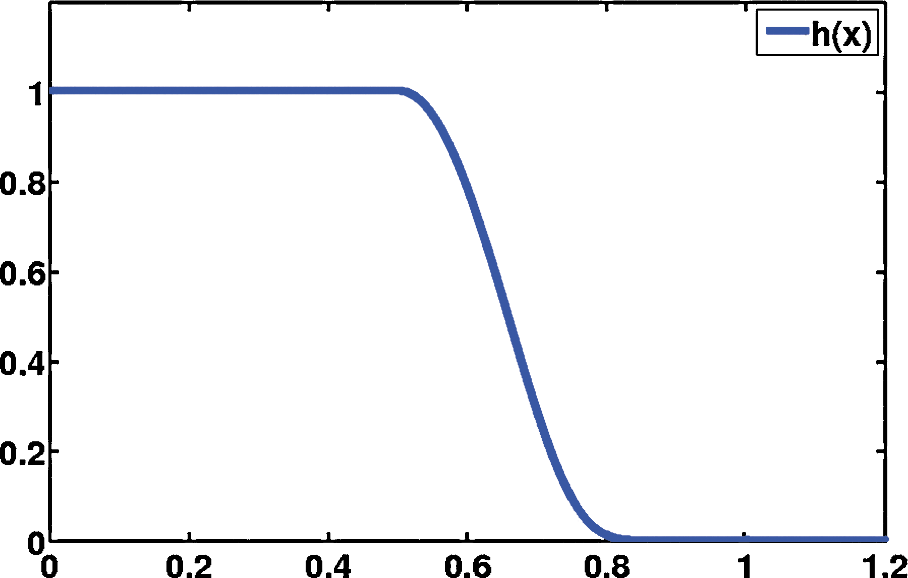
\end{document} → [0, 1] satisfies h(t) = 1 if |t| ≤ 1/2 and h(t) = 0 if |t| ≥ 1, see Figure 1 for a typical function h and Appendix A for a few more technical conditions. Due to the “cut-off” function h, Equation (5) is a finite sum, and ΦN, as a function of only one variable x or y, is contained in ΠN. Under the technical assumptions collected in Appendix A, the estimate
\documentclass{aastex}\usepackage{amsbsy}\usepackage{amsfonts}\usepackage{amssymb}\usepackage{bm}\usepackage{mathrsfs}\usepackage{pifont}\usepackage{stmaryrd}\usepackage{textcomp}\usepackage{portland, xspace}\usepackage{amsmath, amsxtra}\pagestyle{empty}\DeclareMathSizes{10}{9}{7}{6}\begin{document}
\begin{align*}
|\Phi_N (x, y)| {\lesssim} \frac {N^{\alpha}} {\max (1, (N \rho
(x, y))^S}, \tag {6}
\end{align*}
\end{document}
Filter function: A typical filter function h that can be used in Equation (5).
holds, where α is the dimension of \documentclass{aastex}\usepackage{amsbsy}\usepackage{amsfonts}\usepackage{amssymb}\usepackage{bm}\usepackage{mathrsfs}\usepackage{pifont}\usepackage{stmaryrd}\usepackage{textcomp}\usepackage{portland, xspace}\usepackage{amsmath, amsxtra}\pagestyle{empty}\DeclareMathSizes{10}{9}{7}{6}\begin{document}
$${\mathbb X}$$
\end{document}, ρ the metric on \documentclass{aastex}\usepackage{amsbsy}\usepackage{amsfonts}\usepackage{amssymb}\usepackage{bm}\usepackage{mathrsfs}\usepackage{pifont}\usepackage{stmaryrd}\usepackage{textcomp}\usepackage{portland, xspace}\usepackage{amsmath, amsxtra}\pagestyle{empty}\DeclareMathSizes{10}{9}{7}{6}\begin{document}
$${\mathbb X}$$
\end{document}, and S any integer (Filbir and Mhaskar, 2010; Maggioni and Mhaskar, 2008; Mhaskar, 2011). Here means that there is an absolute positive constant on the right-hand side such that the inequality holds. This localization property (6), very much like multi-scale approaches with wavelets, enables local analysis of functions on the manifold.
If f ≈ P, then the we also have \documentclass{aastex}\usepackage{amsbsy}\usepackage{amsfonts}\usepackage{amssymb}\usepackage{bm}\usepackage{mathrsfs}\usepackage{pifont}\usepackage{stmaryrd}\usepackage{textcomp}\usepackage{portland, xspace}\usepackage{amsmath, amsxtra}\pagestyle{empty}\DeclareMathSizes{10}{9}{7}{6}\begin{document}
$$f \Phi_N (x, \cdot) \approx P \Phi_N (x, \cdot)$$
\end{document}. Naturally, we would expect that the product of two polynomials is again a polynomial of a larger degree, so that \documentclass{aastex}\usepackage{amsbsy}\usepackage{amsfonts}\usepackage{amssymb}\usepackage{bm}\usepackage{mathrsfs}\usepackage{pifont}\usepackage{stmaryrd}\usepackage{textcomp}\usepackage{portland, xspace}\usepackage{amsmath, amsxtra}\pagestyle{empty}\DeclareMathSizes{10}{9}{7}{6}\begin{document}
$$P \Phi_N (x, \cdot) \in \Pi_{aN}$$
\end{document}, for some fixed a > 0. Here, we only need the weaker product assumptions. (Appendix A), implying that \documentclass{aastex}\usepackage{amsbsy}\usepackage{amsfonts}\usepackage{amssymb}\usepackage{bm}\usepackage{mathrsfs}\usepackage{pifont}\usepackage{stmaryrd}\usepackage{textcomp}\usepackage{portland, xspace}\usepackage{amsmath, amsxtra}\pagestyle{empty}\DeclareMathSizes{10}{9}{7}{6}\begin{document}
$$P \Phi_N (x, \cdot)$$
\end{document} can be sufficiently well approximated with polynomials in ΠaN. To replace the integral in Equation (4) with a finite sum, we need a quadrature formula that is exact for polynomials up to degree aN: If our data \documentclass{aastex}\usepackage{amsbsy}\usepackage{amsfonts}\usepackage{amssymb}\usepackage{bm}\usepackage{mathrsfs}\usepackage{pifont}\usepackage{stmaryrd}\usepackage{textcomp}\usepackage{portland, xspace}\usepackage{amsmath, amsxtra}\pagestyle{empty}\DeclareMathSizes{10}{9}{7}{6}\begin{document}
$${\cal C} = \{y_i \}_{i = 1}^M$$
\end{document} are sufficiently dense in \documentclass{aastex}\usepackage{amsbsy}\usepackage{amsfonts}\usepackage{amssymb}\usepackage{bm}\usepackage{mathrsfs}\usepackage{pifont}\usepackage{stmaryrd}\usepackage{textcomp}\usepackage{portland, xspace}\usepackage{amsmath, amsxtra}\pagestyle{empty}\DeclareMathSizes{10}{9}{7}{6}\begin{document}
$${\mathbb X}$$
\end{document} (Appendix B), then there are quadrature weights \documentclass{aastex}\usepackage{amsbsy}\usepackage{amsfonts}\usepackage{amssymb}\usepackage{bm}\usepackage{mathrsfs}\usepackage{pifont}\usepackage{stmaryrd}\usepackage{textcomp}\usepackage{portland, xspace}\usepackage{amsmath, amsxtra}\pagestyle{empty}\DeclareMathSizes{10}{9}{7}{6}\begin{document}
$$\{ \omega_i \}_{i = 1}^M$$
\end{document} such that
\documentclass{aastex}\usepackage{amsbsy}\usepackage{amsfonts}\usepackage{amssymb}\usepackage{bm}\usepackage{mathrsfs}\usepackage{pifont}\usepackage{stmaryrd}\usepackage{textcomp}\usepackage{portland, xspace}\usepackage{amsmath, amsxtra}\pagestyle{empty}\DeclareMathSizes{10}{9}{7}{6}\begin{document}
\begin{align*}
\int_{{\mathbb X}} P (x) d \mu (x) = \sum_{j = 1}^M \omega_j P
(x_j), \quad {\rm for \ all} \ P \in \Pi_{aN}.
\end{align*}
\end{document}
Since φ0 ≡ 1, these weights can be computed by solving the linear system of equations
\documentclass{aastex}\usepackage{amsbsy}\usepackage{amsfonts}\usepackage{amssymb}\usepackage{bm}\usepackage{mathrsfs}\usepackage{pifont}\usepackage{stmaryrd}\usepackage{textcomp}\usepackage{portland, xspace}\usepackage{amsmath, amsxtra}\pagestyle{empty}\DeclareMathSizes{10}{9}{7}{6}\begin{document}
\begin{align*}
\sum_{j = 1}^M \omega_j \varphi_k (x_j) = \delta_{k, 0}, \quad{\rm for \ all} \ k = 0, 1, 2, \ldots, aN.
\end{align*}
\end{document}
We refer to Appendix B and Filbir and Mhaskar (2010) for details on the existence of such quadrature weights with respect to the training data.
We now replace the right-hand side of Equation (4) with
\documentclass{aastex}\usepackage{amsbsy}\usepackage{amsfonts}\usepackage{amssymb}\usepackage{bm}\usepackage{mathrsfs}\usepackage{pifont}\usepackage{stmaryrd}\usepackage{textcomp}\usepackage{portland, xspace}\usepackage{amsmath, amsxtra}\pagestyle{empty}\DeclareMathSizes{10}{9}{7}{6}\begin{document}
\begin{align*}
\sigma_N (f, x) : = \sum_{j = 1}^M \omega_jf (y_j) \Phi_N (x, y_j)
. \tag{7}
\end{align*}
\end{document}
To study the asymptotics for N → ∞ , we call for a sequence of training sets \documentclass{aastex}\usepackage{amsbsy}\usepackage{amsfonts}\usepackage{amssymb}\usepackage{bm}\usepackage{mathrsfs}\usepackage{pifont}\usepackage{stmaryrd}\usepackage{textcomp}\usepackage{portland, xspace}\usepackage{amsmath, amsxtra}\pagestyle{empty}\DeclareMathSizes{10}{9}{7}{6}\begin{document}
$${\cal C}_N$$
\end{document} that induce quadrature formulas of strength aN. We shall verify in Appendix C that, for \documentclass{aastex}\usepackage{amsbsy}\usepackage{amsfonts}\usepackage{amssymb}\usepackage{bm}\usepackage{mathrsfs}\usepackage{pifont}\usepackage{stmaryrd}\usepackage{textcomp}\usepackage{portland, xspace}\usepackage{amsmath, amsxtra}\pagestyle{empty}\DeclareMathSizes{10}{9}{7}{6}\begin{document}
$$f \in W^s_{y_0} ({\mathbb X})$$
\end{document}, there is δ > 0, such that,
\documentclass{aastex}\usepackage{amsbsy}\usepackage{amsfonts}\usepackage{amssymb}\usepackage{bm}\usepackage{mathrsfs}\usepackage{pifont}\usepackage{stmaryrd}\usepackage{textcomp}\usepackage{portland, xspace}\usepackage{amsmath, amsxtra}\pagestyle{empty}\DeclareMathSizes{10}{9}{7}{6}\begin{document}
\begin{align*}
\sup_{x \in {B}_\delta (y_0)} \mid\, f (x) - \sigma_{N} (f, x)
\mid \lesssim N^{- s}, \tag{8}
\end{align*}
\end{document}
where \documentclass{aastex}\usepackage{amsbsy}\usepackage{amsfonts}\usepackage{amssymb}\usepackage{bm}\usepackage{mathrsfs}\usepackage{pifont}\usepackage{stmaryrd}\usepackage{textcomp}\usepackage{portland, xspace}\usepackage{amsmath, amsxtra}\pagestyle{empty}\DeclareMathSizes{10}{9}{7}{6}\begin{document}
$${B}_\delta (y_0) \subset {\mathbb X}$$
\end{document}denotes a ball of radius δ around y0. Thus, when f is locally smooth in a neighborhood around y0, then we can locally reconstruct f from the training data. The analogous result for functions that are globally smooth is contained in Filbir and Mhaskar (2010, 2011), Maggioni and Mhaskar (2008), and Mhaskar (2011), which contains local estimates, but the approximand requires global knowledge of f and is not purely defined through the training data only.
4. Specifying φK Numerically
To design a numerically feasible algorithm, we still need to compute a suitable orthonormal basis \documentclass{aastex}\usepackage{amsbsy}\usepackage{amsfonts}\usepackage{amssymb}\usepackage{bm}\usepackage{mathrsfs}\usepackage{pifont}\usepackage{stmaryrd}\usepackage{textcomp}\usepackage{portland, xspace}\usepackage{amsmath, amsxtra}\pagestyle{empty}\DeclareMathSizes{10}{9}{7}{6}\begin{document}
$$\{ \varphi_k \}_{k = 0}^\infty$$
\end{document} for \documentclass{aastex}\usepackage{amsbsy}\usepackage{amsfonts}\usepackage{amssymb}\usepackage{bm}\usepackage{mathrsfs}\usepackage{pifont}\usepackage{stmaryrd}\usepackage{textcomp}\usepackage{portland, xspace}\usepackage{amsmath, amsxtra}\pagestyle{empty}\DeclareMathSizes{10}{9}{7}{6}\begin{document}
$$L_2 ({\mathbb X}, \mu)$$
\end{document}, while the manifold \documentclass{aastex}\usepackage{amsbsy}\usepackage{amsfonts}\usepackage{amssymb}\usepackage{bm}\usepackage{mathrsfs}\usepackage{pifont}\usepackage{stmaryrd}\usepackage{textcomp}\usepackage{portland, xspace}\usepackage{amsmath, amsxtra}\pagestyle{empty}\DeclareMathSizes{10}{9}{7}{6}\begin{document}
$${\mathbb X}$$
\end{document} is not explicitly known to us. In a typical situation, we may have little training data and a much larger but finite collection \documentclass{aastex}\usepackage{amsbsy}\usepackage{amsfonts}\usepackage{amssymb}\usepackage{bm}\usepackage{mathrsfs}\usepackage{pifont}\usepackage{stmaryrd}\usepackage{textcomp}\usepackage{portland, xspace}\usepackage{amsmath, amsxtra}\pagestyle{empty}\DeclareMathSizes{10}{9}{7}{6}\begin{document}
$$\{y_i \}_{i = 1}^M$$
\end{document} of data lying on the manifold. These data shall be used to approximate an orthonormal basis\documentclass{aastex}\usepackage{amsbsy}\usepackage{amsfonts}\usepackage{amssymb}\usepackage{bm}\usepackage{mathrsfs}\usepackage{pifont}\usepackage{stmaryrd}\usepackage{textcomp}\usepackage{portland, xspace}\usepackage{amsmath, amsxtra}\pagestyle{empty}\DeclareMathSizes{10}{9}{7}{6}\begin{document}
$$\{ \varphi_k \}_{k = 0}^\infty$$
\end{document}.
The eigenfunctions of the Laplace-Beltrami operator \documentclass{aastex}\usepackage{amsbsy}\usepackage{amsfonts}\usepackage{amssymb}\usepackage{bm}\usepackage{mathrsfs}\usepackage{pifont}\usepackage{stmaryrd}\usepackage{textcomp}\usepackage{portland, xspace}\usepackage{amsmath, amsxtra}\pagestyle{empty}\DeclareMathSizes{10}{9}{7}{6}\begin{document}
$$\Delta_{\mathbb X} = {\rm div} \nabla$$
\end{document} on the manifold form an orthonormal basis that satisfies the technical assumptions needed in Appendix A. In order to compute them numerically, we build the graph Laplacian from a finite set of points on the manifold as follows: By using data points \documentclass{aastex}\usepackage{amsbsy}\usepackage{amsfonts}\usepackage{amssymb}\usepackage{bm}\usepackage{mathrsfs}\usepackage{pifont}\usepackage{stmaryrd}\usepackage{textcomp}\usepackage{portland, xspace}\usepackage{amsmath, amsxtra}\pagestyle{empty}\DeclareMathSizes{10}{9}{7}{6}\begin{document}
$$\{y_i \}_{i = 1}^M \subset{\mathbb X}$$
\end{document}, the standard heat kernel \documentclass{aastex}\usepackage{amsbsy}\usepackage{amsfonts}\usepackage{amssymb}\usepackage{bm}\usepackage{mathrsfs}\usepackage{pifont}\usepackage{stmaryrd}\usepackage{textcomp}\usepackage{portland, xspace}\usepackage{amsmath, amsxtra}\pagestyle{empty}\DeclareMathSizes{10}{9}{7}{6}\begin{document}
$$k_\varepsilon (x, y) = e^{- \ \parallel x - y \ \parallel^2 / 2 \varepsilon}, \varepsilon > 0$$
\end{document}, induces the weight matrix \documentclass{aastex}\usepackage{amsbsy}\usepackage{amsfonts}\usepackage{amssymb}\usepackage{bm}\usepackage{mathrsfs}\usepackage{pifont}\usepackage{stmaryrd}\usepackage{textcomp}\usepackage{portland, xspace}\usepackage{amsmath, amsxtra}\pagestyle{empty}\DeclareMathSizes{10}{9}{7}{6}\begin{document}
$${\cal W}^{\varepsilon}_M$$
\end{document} defined by \documentclass{aastex}\usepackage{amsbsy}\usepackage{amsfonts}\usepackage{amssymb}\usepackage{bm}\usepackage{mathrsfs}\usepackage{pifont}\usepackage{stmaryrd}\usepackage{textcomp}\usepackage{portland, xspace}\usepackage{amsmath, amsxtra}\pagestyle{empty}\DeclareMathSizes{10}{9}{7}{6}\begin{document}
$${\cal W}^{\varepsilon}_{M;i, j} = k_\varepsilon (y_i, y_j)$$
\end{document}. We build the diagonal matrix \documentclass{aastex}\usepackage{amsbsy}\usepackage{amsfonts}\usepackage{amssymb}\usepackage{bm}\usepackage{mathrsfs}\usepackage{pifont}\usepackage{stmaryrd}\usepackage{textcomp}\usepackage{portland, xspace}\usepackage{amsmath, amsxtra}\pagestyle{empty}\DeclareMathSizes{10}{9}{7}{6}\begin{document}
$$D^{\varepsilon}_{M;i, i} = \sum\nolimits_{j = 1}^M {\cal W}^{\varepsilon}_{M;i, j}$$
\end{document} and define the (unnormalized) graph Laplacian as \documentclass{aastex}\usepackage{amsbsy}\usepackage{amsfonts}\usepackage{amssymb}\usepackage{bm}\usepackage{mathrsfs}\usepackage{pifont}\usepackage{stmaryrd}\usepackage{textcomp}\usepackage{portland, xspace}\usepackage{amsmath, amsxtra}\pagestyle{empty}\DeclareMathSizes{10}{9}{7}{6}\begin{document}
$$L^{\varepsilon}_M = {\cal W}^{\varepsilon}_M - D^{\varepsilon}_M$$
\end{document}. For M → ∞ and ɛ → 0, the eigenvalues and interpolations of the eigenvectors of \documentclass{aastex}\usepackage{amsbsy}\usepackage{amsfonts}\usepackage{amssymb}\usepackage{bm}\usepackage{mathrsfs}\usepackage{pifont}\usepackage{stmaryrd}\usepackage{textcomp}\usepackage{portland, xspace}\usepackage{amsmath, amsxtra}\pagestyle{empty}\DeclareMathSizes{10}{9}{7}{6}\begin{document}
$$L_M^\epsilon$$
\end{document}converge toward the “interesting” eigenvalues and eigenfunctions of \documentclass{aastex}\usepackage{amsbsy}\usepackage{amsfonts}\usepackage{amssymb}\usepackage{bm}\usepackage{mathrsfs}\usepackage{pifont}\usepackage{stmaryrd}\usepackage{textcomp}\usepackage{portland, xspace}\usepackage{amsmath, amsxtra}\pagestyle{empty}\DeclareMathSizes{10}{9}{7}{6}\begin{document}
$$\Delta_{\mathbb X}$$
\end{document} when \documentclass{aastex}\usepackage{amsbsy}\usepackage{amsfonts}\usepackage{amssymb}\usepackage{bm}\usepackage{mathrsfs}\usepackage{pifont}\usepackage{stmaryrd}\usepackage{textcomp}\usepackage{portland, xspace}\usepackage{amsmath, amsxtra}\pagestyle{empty}\DeclareMathSizes{10}{9}{7}{6}\begin{document}
$$\{y_i \}_{i = 1}^M$$
\end{document}are uniformly distributed on \documentclass{aastex}\usepackage{amsbsy}\usepackage{amsfonts}\usepackage{amssymb}\usepackage{bm}\usepackage{mathrsfs}\usepackage{pifont}\usepackage{stmaryrd}\usepackage{textcomp}\usepackage{portland, xspace}\usepackage{amsmath, amsxtra}\pagestyle{empty}\DeclareMathSizes{10}{9}{7}{6}\begin{document}
$${\mathbb X}$$
\end{document}. See Appendix D for the details and technical assumptions. If \documentclass{aastex}\usepackage{amsbsy}\usepackage{amsfonts}\usepackage{amssymb}\usepackage{bm}\usepackage{mathrsfs}\usepackage{pifont}\usepackage{stmaryrd}\usepackage{textcomp}\usepackage{portland, xspace}\usepackage{amsmath, amsxtra}\pagestyle{empty}\DeclareMathSizes{10}{9}{7}{6}\begin{document}
$$\{y_i \}_{i = 1}^M$$
\end{document} are distributed according to the density p, then the graph Laplacian approximates the elliptic Schrödinger-type operator \documentclass{aastex}\usepackage{amsbsy}\usepackage{amsfonts}\usepackage{amssymb}\usepackage{bm}\usepackage{mathrsfs}\usepackage{pifont}\usepackage{stmaryrd}\usepackage{textcomp}\usepackage{portland, xspace}\usepackage{amsmath, amsxtra}\pagestyle{empty}\DeclareMathSizes{10}{9}{7}{6}\begin{document}
$$\Delta + \frac {\Delta p} {p} $$
\end{document} (Coifman et al., 2005b; Nadler et al., 2006), whose eigenfunctions also form an orthonormal basis for \documentclass{aastex}\usepackage{amsbsy}\usepackage{amsfonts}\usepackage{amssymb}\usepackage{bm}\usepackage{mathrsfs}\usepackage{pifont}\usepackage{stmaryrd}\usepackage{textcomp}\usepackage{portland, xspace}\usepackage{amsmath, amsxtra}\pagestyle{empty}\DeclareMathSizes{10}{9}{7}{6}\begin{document}
$$L_2 ({\mathbb X}, \mu)$$
\end{document}.
5. Localized Kernels on the Sphere
The data of one of our applications lie on the sphere Sd−1, so that we specify our approach for \documentclass{aastex}\usepackage{amsbsy}\usepackage{amsfonts}\usepackage{amssymb}\usepackage{bm}\usepackage{mathrsfs}\usepackage{pifont}\usepackage{stmaryrd}\usepackage{textcomp}\usepackage{portland, xspace}\usepackage{amsmath, amsxtra}\pagestyle{empty}\DeclareMathSizes{10}{9}{7}{6}\begin{document}
$${\mathbb X} = S^{d - 1}$$
\end{document} (Gia and Mhaskar, 2006; Gia and Mhaskar, 2008b). For \documentclass{aastex}\usepackage{amsbsy}\usepackage{amsfonts}\usepackage{amssymb}\usepackage{bm}\usepackage{mathrsfs}\usepackage{pifont}\usepackage{stmaryrd}\usepackage{textcomp}\usepackage{portland, xspace}\usepackage{amsmath, amsxtra}\pagestyle{empty}\DeclareMathSizes{10}{9}{7}{6}\begin{document}
$$f:S^{d - 1} \rightarrow {\rm R}, \ {\rm let} \ \check{f} (x) : = f (x / \ \parallel x \ \parallel)$$
\end{document} be its extension to \documentclass{aastex}\usepackage{amsbsy}\usepackage{amsfonts}\usepackage{amssymb}\usepackage{bm}\usepackage{mathrsfs}\usepackage{pifont}\usepackage{stmaryrd}\usepackage{textcomp}\usepackage{portland, xspace}\usepackage{amsmath, amsxtra}\pagestyle{empty}\DeclareMathSizes{10}{9}{7}{6}\begin{document}
$${\mathbb R}^d \backslash \{0 \} $$
\end{document}. The Laplace-Beltrami operator \documentclass{aastex}\usepackage{amsbsy}\usepackage{amsfonts}\usepackage{amssymb}\usepackage{bm}\usepackage{mathrsfs}\usepackage{pifont}\usepackage{stmaryrd}\usepackage{textcomp}\usepackage{portland, xspace}\usepackage{amsmath, amsxtra}\pagestyle{empty}\DeclareMathSizes{10}{9}{7}{6}\begin{document}
$$\Delta_{S^{d - 1}} \ {\rm is} \ \Delta_{S^{d - 1}} f = (\Delta_{\rm R^d} \check{f})_{\mid S^{d - 1}}$$
\end{document}, and the set of spherical harmonics \documentclass{aastex}\usepackage{amsbsy}\usepackage{amsfonts}\usepackage{amssymb}\usepackage{bm}\usepackage{mathrsfs}\usepackage{pifont}\usepackage{stmaryrd}\usepackage{textcomp}\usepackage{portland, xspace}\usepackage{amsmath, amsxtra}\pagestyle{empty}\DeclareMathSizes{10}{9}{7}{6}\begin{document}
$${\cal H}^d_k$$
\end{document} is formed by the homogeneous harmonic polynomials p on \documentclass{aastex}\usepackage{amsbsy}\usepackage{amsfonts}\usepackage{amssymb}\usepackage{bm}\usepackage{mathrsfs}\usepackage{pifont}\usepackage{stmaryrd}\usepackage{textcomp}\usepackage{portland, xspace}\usepackage{amsmath, amsxtra}\pagestyle{empty}\DeclareMathSizes{10}{9}{7}{6}\begin{document}
$${\mathbb R}^d$$
\end{document}of degree k restricted onto the sphere Sd−1. In other words, p is a polynomial whose monomials have all the same total degree k and\documentclass{aastex}\usepackage{amsbsy}\usepackage{amsfonts}\usepackage{amssymb}\usepackage{bm}\usepackage{mathrsfs}\usepackage{pifont}\usepackage{stmaryrd}\usepackage{textcomp}\usepackage{portland, xspace}\usepackage{amsmath, amsxtra}\pagestyle{empty}\DeclareMathSizes{10}{9}{7}{6}\begin{document}
$$\Delta_{{\mathbb R}^d}p = 0.$$
\end{document} The eigenspaces of \documentclass{aastex}\usepackage{amsbsy}\usepackage{amsfonts}\usepackage{amssymb}\usepackage{bm}\usepackage{mathrsfs}\usepackage{pifont}\usepackage{stmaryrd}\usepackage{textcomp}\usepackage{portland, xspace}\usepackage{amsmath, amsxtra}\pagestyle{empty}\DeclareMathSizes{10}{9}{7}{6}\begin{document}
$$\Delta_{S^{d - 1}}$$
\end{document} are \documentclass{aastex}\usepackage{amsbsy}\usepackage{amsfonts}\usepackage{amssymb}\usepackage{bm}\usepackage{mathrsfs}\usepackage{pifont}\usepackage{stmaryrd}\usepackage{textcomp}\usepackage{portland, xspace}\usepackage{amsmath, amsxtra}\pagestyle{empty}\DeclareMathSizes{10}{9}{7}{6}\begin{document}
$${\cal H}^d_k$$
\end{document} with eigenvalues k(k + d − 2), respectively, and the dimension of \documentclass{aastex}\usepackage{amsbsy}\usepackage{amsfonts}\usepackage{amssymb}\usepackage{bm}\usepackage{mathrsfs}\usepackage{pifont}\usepackage{stmaryrd}\usepackage{textcomp}\usepackage{portland, xspace}\usepackage{amsmath, amsxtra}\pagestyle{empty}\DeclareMathSizes{10}{9}{7}{6}\begin{document}
$${\cal H}^d_k$$
\end{document} is mk := \documentclass{aastex}\usepackage{amsbsy}\usepackage{amsfonts}\usepackage{amssymb}\usepackage{bm}\usepackage{mathrsfs}\usepackage{pifont}\usepackage{stmaryrd}\usepackage{textcomp}\usepackage{portland, xspace}\usepackage{amsmath, amsxtra}\pagestyle{empty}\DeclareMathSizes{10}{9}{7}{6}\begin{document}
$${k + d - 1 \choose k} - {k + d - 3 \choose k - 2}$$
\end{document}. If we choose an orthonormal basis \documentclass{aastex}\usepackage{amsbsy}\usepackage{amsfonts}\usepackage{amssymb}\usepackage{bm}\usepackage{mathrsfs}\usepackage{pifont}\usepackage{stmaryrd}\usepackage{textcomp}\usepackage{portland, xspace}\usepackage{amsmath, amsxtra}\pagestyle{empty}\DeclareMathSizes{10}{9}{7}{6}\begin{document}
$$\{ \varphi_{k, j} \}_{j = 1}^{m_k}$$
\end{document} for \documentclass{aastex}\usepackage{amsbsy}\usepackage{amsfonts}\usepackage{amssymb}\usepackage{bm}\usepackage{mathrsfs}\usepackage{pifont}\usepackage{stmaryrd}\usepackage{textcomp}\usepackage{portland, xspace}\usepackage{amsmath, amsxtra}\pagestyle{empty}\DeclareMathSizes{10}{9}{7}{6}\begin{document}
$${\cal H}^d_k$$
\end{document}, then \documentclass{aastex}\usepackage{amsbsy}\usepackage{amsfonts}\usepackage{amssymb}\usepackage{bm}\usepackage{mathrsfs}\usepackage{pifont}\usepackage{stmaryrd}\usepackage{textcomp}\usepackage{portland, xspace}\usepackage{amsmath, amsxtra}\pagestyle{empty}\DeclareMathSizes{10}{9}{7}{6}\begin{document}
$$\sum\nolimits_{j = 1}^{m_k} \varphi_{k, j} (x) \varphi_{k, j} (y)$$
\end{document} does not depend on the choice of \documentclass{aastex}\usepackage{amsbsy}\usepackage{amsfonts}\usepackage{amssymb}\usepackage{bm}\usepackage{mathrsfs}\usepackage{pifont}\usepackage{stmaryrd}\usepackage{textcomp}\usepackage{portland, xspace}\usepackage{amsmath, amsxtra}\pagestyle{empty}\DeclareMathSizes{10}{9}{7}{6}\begin{document}
$$\{ \varphi_{k, j} \}_{j = 1}^{m_k}$$
\end{document} and coincides with \documentclass{aastex}\usepackage{amsbsy}\usepackage{amsfonts}\usepackage{amssymb}\usepackage{bm}\usepackage{mathrsfs}\usepackage{pifont}\usepackage{stmaryrd}\usepackage{textcomp}\usepackage{portland, xspace}\usepackage{amsmath, amsxtra}\pagestyle{empty}\DeclareMathSizes{10}{9}{7}{6}\begin{document}
$$P_k (\langle x, y \rangle)$$
\end{document}, where Pk is the Gegenbauer polynomial of degree k and parameter d/2 − 1, sec. Appendix E.1 and Stein and Weiss (1971). Therefore, we can explicitly compute
\documentclass{aastex}\usepackage{amsbsy}\usepackage{amsfonts}\usepackage{amssymb}\usepackage{bm}\usepackage{mathrsfs}\usepackage{pifont}\usepackage{stmaryrd}\usepackage{textcomp}\usepackage{portland, xspace}\usepackage{amsmath, amsxtra}\pagestyle{empty}\DeclareMathSizes{10}{9}{7}{6}\begin{document}
\begin{align*}
\Phi_N (x, y) = \sum_{k = 0}^N h \bigg (\frac {\sqrt {k (k + d -
2)}} {N} \bigg) P_k (\langle x, y \rangle) .
\end{align*}
\end{document}
To derive σN(f,x) in Equation (7), we still need to determine the quadrature weights \documentclass{aastex}\usepackage{amsbsy}\usepackage{amsfonts}\usepackage{amssymb}\usepackage{bm}\usepackage{mathrsfs}\usepackage{pifont}\usepackage{stmaryrd}\usepackage{textcomp}\usepackage{portland, xspace}\usepackage{amsmath, amsxtra}\pagestyle{empty}\DeclareMathSizes{10}{9}{7}{6}\begin{document}
$$\{ \omega_j \}_{j = 1}^n$$
\end{document}, which we shall properly describe in Appendix E.2. Here, we only present a heuristic approach. Since \documentclass{aastex}\usepackage{amsbsy}\usepackage{amsfonts}\usepackage{amssymb}\usepackage{bm}\usepackage{mathrsfs}\usepackage{pifont}\usepackage{stmaryrd}\usepackage{textcomp}\usepackage{portland, xspace}\usepackage{amsmath, amsxtra}\pagestyle{empty}\DeclareMathSizes{10}{9}{7}{6}\begin{document}
$$\{P_k (\langle x, \cdot \rangle) \}_{x \in S^{d - 1}}$$
\end{document} generates \documentclass{aastex}\usepackage{amsbsy}\usepackage{amsfonts}\usepackage{amssymb}\usepackage{bm}\usepackage{mathrsfs}\usepackage{pifont}\usepackage{stmaryrd}\usepackage{textcomp}\usepackage{portland, xspace}\usepackage{amsmath, amsxtra}\pagestyle{empty}\DeclareMathSizes{10}{9}{7}{6}\begin{document}
$${\cal H}^d_k$$
\end{document}, we aim to solve, for R as large as possible,
\documentclass{aastex}\usepackage{amsbsy}\usepackage{amsfonts}\usepackage{amssymb}\usepackage{bm}\usepackage{mathrsfs}\usepackage{pifont}\usepackage{stmaryrd}\usepackage{textcomp}\usepackage{portland, xspace}\usepackage{amsmath, amsxtra}\pagestyle{empty}\DeclareMathSizes{10}{9}{7}{6}\begin{document}
\begin{align*}
\sum_{j = 1}^n \omega_j P_k (\langle x, x_j \rangle) = \delta_{k, 0}, \qquad {\rm for \ all} \ k = 0, \ldots, R,
\end{align*}
\end{document}
and mk = dim \documentclass{aastex}\usepackage{amsbsy}\usepackage{amsfonts}\usepackage{amssymb}\usepackage{bm}\usepackage{mathrsfs}\usepackage{pifont}\usepackage{stmaryrd}\usepackage{textcomp}\usepackage{portland, xspace}\usepackage{amsmath, amsxtra}\pagestyle{empty}\DeclareMathSizes{10}{9}{7}{6}\begin{document}
$$({\cal H}^d_k)$$
\end{document} random choices of \documentclass{aastex}\usepackage{amsbsy}\usepackage{amsfonts}\usepackage{amssymb}\usepackage{bm}\usepackage{mathrsfs}\usepackage{pifont}\usepackage{stmaryrd}\usepackage{textcomp}\usepackage{portland, xspace}\usepackage{amsmath, amsxtra}\pagestyle{empty}\DeclareMathSizes{10}{9}{7}{6}\begin{document}
$$x \in S^{d - 1}$$
\end{document}. This leads to a linear system of equations whose solution is reasonably close to exact weights in practice, but only for small parameters d, n, and R. If any of these parameters is not small, then the problem becomes numerically unstable, and we need to follow the approach presented in Appendix E.
If the manifold is known, as in the case of the sphere, many types of basis functions can be constructed explicitly. For instance, spherical wavelets were considered in Antoine and Vandergheynst (1995), Dahlke et al. (1995, 2004), and Starck et al. (2006), which can capture multi-scale structure. However, replacing the eigenfunctions \documentclass{aastex}\usepackage{amsbsy}\usepackage{amsfonts}\usepackage{amssymb}\usepackage{bm}\usepackage{mathrsfs}\usepackage{pifont}\usepackage{stmaryrd}\usepackage{textcomp}\usepackage{portland, xspace}\usepackage{amsmath, amsxtra}\pagestyle{empty}\DeclareMathSizes{10}{9}{7}{6}\begin{document}
$$\{ \varphi_k \}_{k = 0}^\infty$$
\end{document} of the Laplace-Beltrami operator would require checking in each case if all the conditions in Appendix A are satisfied. Therefore, we shall not follow this path and, here, exclusively use the eigenfunctions of the Laplace-Beltrami operator.
6. Applications
We use the developed approximation scheme to cluster biomedical data into disease stages \documentclass{aastex}\usepackage{amsbsy}\usepackage{amsfonts}\usepackage{amssymb}\usepackage{bm}\usepackage{mathrsfs}\usepackage{pifont}\usepackage{stmaryrd}\usepackage{textcomp}\usepackage{portland, xspace}\usepackage{amsmath, amsxtra}\pagestyle{empty}\DeclareMathSizes{10}{9}{7}{6}\begin{document}
$$\{C_l \}_{l = 0}^L$$
\end{document}. Therefore, the classes (disease stages) have a natural ordering, and we assign a meaningful number cl to cluster Cl such that \documentclass{aastex}\usepackage{amsbsy}\usepackage{amsfonts}\usepackage{amssymb}\usepackage{bm}\usepackage{mathrsfs}\usepackage{pifont}\usepackage{stmaryrd}\usepackage{textcomp}\usepackage{portland, xspace}\usepackage{amsmath, amsxtra}\pagestyle{empty}\DeclareMathSizes{10}{9}{7}{6}\begin{document}
$$0 \leq c_0 < c_1 < \ldots < c_L$$
\end{document}. Hence, |ci −cj| represents the distance between Ci and Cj. The query function f is defined on the training data by f (xi) = cl if and only if \documentclass{aastex}\usepackage{amsbsy}\usepackage{amsfonts}\usepackage{amssymb}\usepackage{bm}\usepackage{mathrsfs}\usepackage{pifont}\usepackage{stmaryrd}\usepackage{textcomp}\usepackage{portland, xspace}\usepackage{amsmath, amsxtra}\pagestyle{empty}\DeclareMathSizes{10}{9}{7}{6}\begin{document}
$$x_i \in C_l$$
\end{document}. The approximand σN(f,x) induces a nearest neighbor classification on the entire dataset by the proximity of σN(f,x) to any of the numbers \documentclass{aastex}\usepackage{amsbsy}\usepackage{amsfonts}\usepackage{amssymb}\usepackage{bm}\usepackage{mathrsfs}\usepackage{pifont}\usepackage{stmaryrd}\usepackage{textcomp}\usepackage{portland, xspace}\usepackage{amsmath, amsxtra}\pagestyle{empty}\DeclareMathSizes{10}{9}{7}{6}\begin{document}
$$c_0, \ldots, c_L$$
\end{document}.
We first compare our proposed approach to widely used classification methods on two standard biomedical datasets. After this verification, we use our scheme to analyze multispectral retinal images of age-related macular degeneration (AMD) patients. All eye-related data were collected by our collaborators at the National Eye Clinic at the National Institutes of Health (Bethesda, NIH; Maryland).
The Cleveland Heart Disease Database (CHDD) (Detrano et al., 1989) contains 297 patterns with 13 attributes and is grouped into five progressive heart disease stages (values 0,1,2,3,4), where 0 corresponds to normal heart conditions. We removed six patterns due to missing values. Due to homeostasis and its failure in progressed disease, we expect the query function f to be smoother on normal heart conditions and early disease stages, while later stages may form a more heterogeneous group. We compare our method to support vector machines (SVM), in which clusters are derived through sequential binary clustering. Clusters are evaluated by means of binary false-positive or false-negatives for each disease stage. Indeed, our proposed method recovers f consistently better than SVM for the values 0, 1, and 2 when dealing with few training points (Table 1). As expected, our kernel performs poorly on the stages 3 and 4, implying the lack of smoothness of f within these progressed stages. The transition from 0 to 2 seems to be steered by a smoother process, which is reflected by a smoother query function yielding better results than SVM methods.
Sensitivity Analysis for Cleveland Heart Disease Database
Stage 0
SVM linear
SVM Gaussian
Local kernel
CHDD, 40
73%
71%
79%
CHDD, 100
78%
80%
83%
CHDD, 200
93%
95%
92%
Stage 1
CHDD, 40
69%
68%
73%
CHDD, 100
73%
75%
80%
CHDD, 200
88%
92%
85%
Stage 2
CHDD, 40
64%
62%
71%
CHDD, 100
68%
71%
75%
CHDD, 200
86%
85%
81%
Stage 3
CHDD, 40
61%
60%
54%
CHDD, 100
65%
66%
59%
CHDD, 200
78%
79%
69%
Stage 4
CHDD, 40
57%
55%
52%
CHDD, 100
63%
59%
54%
CHDD, 200
72%
69%
63%
Sensitivity (one minus false negative rate) for disease stages 0 to 4 using the dataset CHDD in Section 6.1.1. with 40, 100, and 200 training points, averaged over 50 instances for each method. Our local kernel method performs better for few training data than SVM on disease stages 0, 1, and 2, in which we expect the query function to be relatively smooth. CHDD, Cleveland Heart Disease Database.
6.1.2. Wisconsin Breast Cancer Database: data completion
After removing missing values, the Wisconsin Breast Cancer Database (WBCD; original) (Wolberg and Mangasarian, 1990) contains 683 patterns with 9 attributes. We aim to predict quantitative attributes. In fact, we randomly select 200, 300, and 400 training points to learn the attribute “clump thickness” (ranging from 1 to 10) and aim to predict its values on the remaining data. We call it a hit when the prediction is within a radius of 1, i.e., if the measured size was 3, the predictions in the interval [2, 4] are counted as a hit. The excellent performance of our proposed method by means of sensitivity (number of hits divided by the cluster size) for few training data is shown in Table 2.
Sensitivity Analysis for the Wisconsin Breast Cancer Database
SVM linear
SVM Gaussian
Local kernel
WBCD, 100
74%
72%
80%
WBCD, 200
76%
79%
84%
WBCD, 300
92%
93%
90%
Sensitivity analysis for the data set WBCD in Section 6.1.2, averaged over clump thickness and 50 instances for each method. Our local kernel method yields high sensitivity compared to other methods when there are only few training data. WBCD, Wisconsin Breast Cancer Database.
6.2. Age-related macular degeneration
Age-related macular degeneration is the most common cause of blindness among the elderly population in the western world (Chew et al., 2009; Coleman et al., 2008; Krishnadev et al., 2010). Aging of the human retina is universally associated with microscopic changes within the retinal pigment epithelium (RPE), including increased number and volume of fluorescent lipofuscin granules (Meyers et al., 2004). In a majority of Americans over the age of 60, the earliest clinical signs of RPE dysfunction are observed in color fundus photographs as drusen—bright highly reflective extracellular deposits between the RPE and its basement membrane. Macular drusen increase in number and size with advancing age in epidemiological studies and larger, irregular-shaped, perifoveal drusen (“soft”) are considered to confer the greatest risk for progression to advanced AMD. Through many years of large-scale studies of the natural history of AMD and controlled prevention trials, clinical observations of fundus photographs suggest that people with soft (larger than 150 microns and irregularly shaped) drusen are at high risk for progressing to advanced AMD. Currently, pathologists in reading centers classify drusen based on size and shape (Bird et al., 1995) in reflection color fundus images. There is demand for automated analysis tools that allow for quantitative prediction of disease progression.
6.2.1. Retinal multi-spectral imaging
The retina is a multilayer neural tissue, uniquely suited for noninvasive optical imaging with high resolution. The first author, together with his collaborators at NIH, developed noninvasive multispectral fluorescence imaging of the human retina by adding selected interference filter sets to standard fundus cameras, allowing the monitoring of early changes within the RPE via the fluorescent lipofuscin granules (Dobrosotskaya et al., 2010, 2011; Ehler et al., 2010, 2011a, 2011b; Kainerstorfer et al., 2010a, 2010b, 2011). If F(Λ,λ) denotes the measured autofluorescence, where Λ is the excitation and λ the emission wavelength, then the Beer-Lambert law for the double-path yields
\documentclass{aastex}\usepackage{amsbsy}\usepackage{amsfonts}\usepackage{amssymb}\usepackage{bm}\usepackage{mathrsfs}\usepackage{pifont}\usepackage{stmaryrd}\usepackage{textcomp}\usepackage{portland, xspace}\usepackage{amsmath, amsxtra}\pagestyle{empty}\DeclareMathSizes{10}{9}{7}{6}\begin{document}
\begin{align*}
F (\Lambda, \lambda) = I (\Lambda) \Phi (\Lambda, \lambda) e^{- (D (\Lambda) + D (\lambda))},
\end{align*}
\end{document}
where D is the integrated absorbance (optical density) of the tissue the light travels through, Φ(Λ,λ) is the fluorescence efficiency of lipofuscin, and I(Λ) the radiant power of the excitation light. For each of the six patients, four excitation filters with two emission filters and trifold imaging lead to 24 images (400 × 400 pixels) that are aligned by applying the commercial software i2k Align. We de-noise in z-direction by principal component analysis, keeping five eigenvectors capturing more than 98% of the dataset's variance. Spatial noise is reduced by averaging each pixel with its eight neighbors. Since the pathological changes are related to fractional changes of the autofluorescence, we can normalize the 160,000 vectors to lie on the sphere S4.
The principal component analysis and normalization also helps to compare pixels across patients. The drusen classification scheme presented in van Leeuwen et al. (2003; see also Bird et al., 1995) leads to 8 progressing stages. We partition them into four classes. An expert grader labeled few spatial regions, which led to 2,000 training pixels in three patients that were each labeled with one of the four partitions. Thus, we have 6,000 training vectors total, and pixels in a single patient can have distinct labels. We shall learn locally the pixel classification into drusen classes. Note that our method relies on the multispectral components of drusen in autofluorescence images rather than the spatial shape that is seen in reflection color fundus images.
After the learning step, we mark a region of interest (ROI) in six patients (including the three patients used for learning). To classify pixels from the ROI into the four partitions, we merge the ROI pixels of the patient under consideration with the ROI pixels of the three learned patients to form the data on the manifold. The labeled regions are the training data, and since the pixel vectors lie on the sphere, we can follow the approach in Section 5 to derive σN(f, x) (Fig. 2). The majority of the pixels within the ROI would define the drusen class of the patient. It should be mentioned that the size of the ROI influences the classification scheme, and we obtained good results with the center in the fovea and extending to 5 degrees, consistent with common image analysis in ophthalmology.
Drusen classification. The foveal class outnumbers the other classes in (d) and determines the patient's class. (a, left) Drusen in color fundus image; (a, right) Drusen in cross-section of a monkey retina. (b) Two spectral images of pre-advanced AMD patient. (c) Two spectral images of advanced AMD patient. (d, left) Squares show class centers; (d, right) four classes, where dark blue is not assigned to any class.
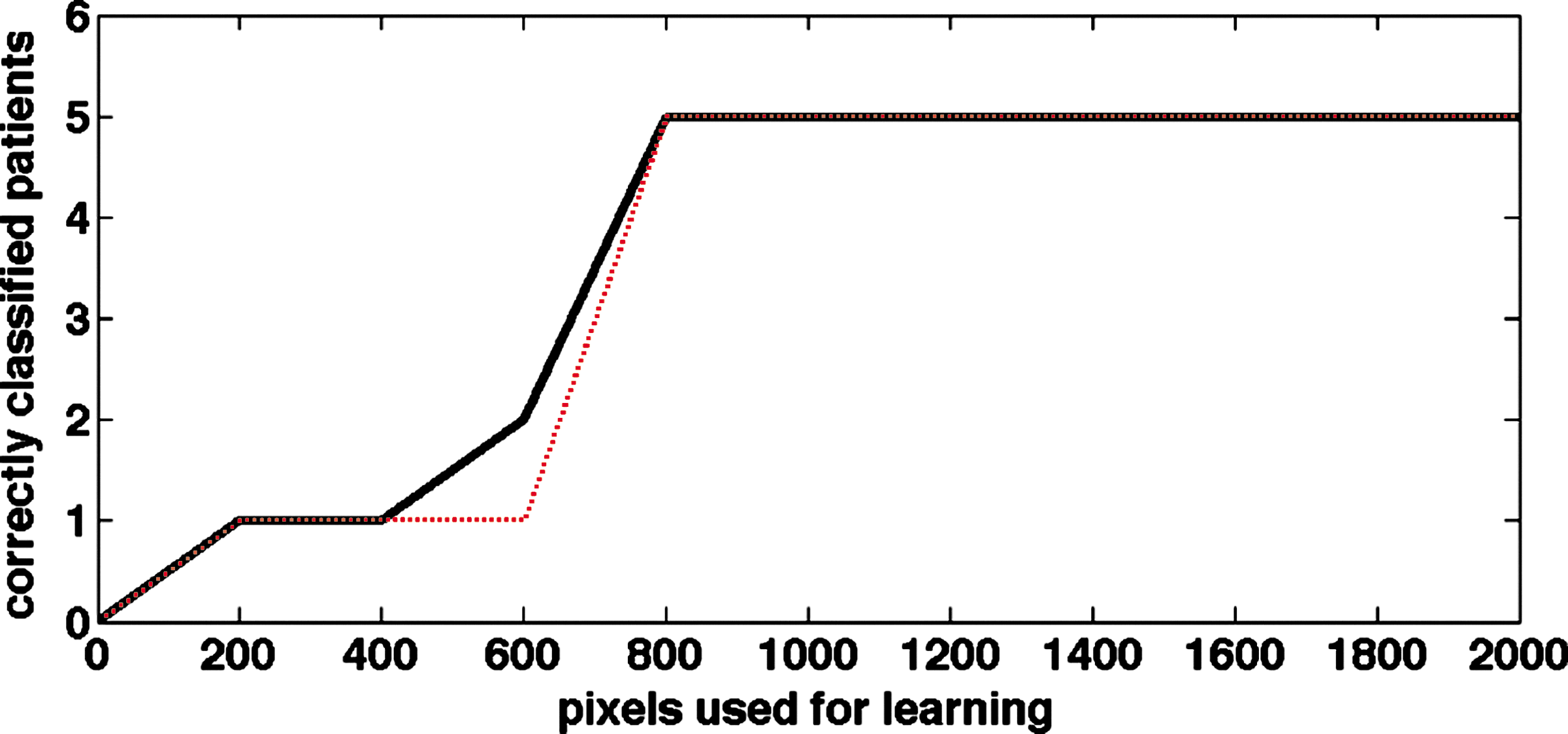
Next, we explore the influence of the size of the training data. We only use a fraction of the pixels that were originally labeled by our grader. The individual pixels are selected by a random sampling. Figure 3 shows that we require a critical number of training pixels and from there on, we obtain stable classification results.
The increments of the training pixels are in steps of 200. The y-axis counts the correct classifications. Note that we simply removed random pixels from the entire set of 3 × 2000 training pixels, so that each smaller training set is contained in the larger one. We repeated this process over 20 runs to avoid random anomalies, which led to the black curve. The most typical curve in a single run is depicted in red. For few training data, we only classify one single patient correctly. Increasing the size of the training pixels enables consistently correct classifications of all but one patient (consistently the same one). It seems that the critical number of training pixels is between 600 and 800 pixels.
7. Conclusions
To facilitate the analysis of complex biomedical data, we developed the mathematical foundations for a numerical algorithm that enables global and local data analysis integratively. After we validated our approach on two standard datasets, we aimed to classify and predict disease progression in AMD patients. Drusen were classified in multispectral retinal image sets that enabled quantitative measurements of advanced pathological changes. Clearly, our new mathematical approach to identifying new components controlling AMD progression is preliminary and needs further validation to claim its usefulness in general terms. We anticipate improvements through synergies of multiple analysis schemes with multi modal data so that our proposed analysis could be part of an iterative process.
8. Appendix
Appendix A. Technical assumptions
For the sake of readability, we list simple conditions used in Section 3 that can be further weakened (Filbir and Mhaskar, 2010; Maggioni and Mhaskar, 2008). The manifold \documentclass{aastex}\usepackage{amsbsy}\usepackage{amsfonts}\usepackage{amssymb}\usepackage{bm}\usepackage{mathrsfs}\usepackage{pifont}\usepackage{stmaryrd}\usepackage{textcomp}\usepackage{portland, xspace}\usepackage{amsmath, amsxtra}\pagestyle{empty}\DeclareMathSizes{10}{9}{7}{6}\begin{document}
$${\mathbb X}$$
\end{document} is supposed to be a smooth, compact, and connected Riemannian manifold without boundary. We point out that the following technical conditions are satisfied when \documentclass{aastex}\usepackage{amsbsy}\usepackage{amsfonts}\usepackage{amssymb}\usepackage{bm}\usepackage{mathrsfs}\usepackage{pifont}\usepackage{stmaryrd}\usepackage{textcomp}\usepackage{portland, xspace}\usepackage{amsmath, amsxtra}\pagestyle{empty}\DeclareMathSizes{10}{9}{7}{6}\begin{document}
$$\{ \varphi_k \}_{k = 0}^\infty$$
\end{document} are the eigenfunctions of the Laplace-Beltrami operator on \documentclass{aastex}\usepackage{amsbsy}\usepackage{amsfonts}\usepackage{amssymb}\usepackage{bm}\usepackage{mathrsfs}\usepackage{pifont}\usepackage{stmaryrd}\usepackage{textcomp}\usepackage{portland, xspace}\usepackage{amsmath, amsxtra}\pagestyle{empty}\DeclareMathSizes{10}{9}{7}{6}\begin{document}
$${\mathbb X}, \{ \ell^2_k \}_{k = 0}^\infty$$
\end{document} its eigenvalues, and μ the standard Riemannian probability measure (see Filbir and Mhaskar, 2010, 2011; Maggioni and Mhaskar, 2008; Sikora, 2004 for details).
A.1. Assumption on the volume of balls
If α > 0 is the dimension of \documentclass{aastex}\usepackage{amsbsy}\usepackage{amsfonts}\usepackage{amssymb}\usepackage{bm}\usepackage{mathrsfs}\usepackage{pifont}\usepackage{stmaryrd}\usepackage{textcomp}\usepackage{portland, xspace}\usepackage{amsmath, amsxtra}\pagestyle{empty}\DeclareMathSizes{10}{9}{7}{6}\begin{document}
$${\mathbb X}$$
\end{document}, then we assume that μ(Br(x))⪅rα, for all \documentclass{aastex}\usepackage{amsbsy}\usepackage{amsfonts}\usepackage{amssymb}\usepackage{bm}\usepackage{mathrsfs}\usepackage{pifont}\usepackage{stmaryrd}\usepackage{textcomp}\usepackage{portland, xspace}\usepackage{amsmath, amsxtra}\pagestyle{empty}\DeclareMathSizes{10}{9}{7}{6}\begin{document}
$$x \in {\mathbb X}$$
\end{document} and r > 0.
A.2. Assumption on products of polynomials
There is a ≥ 2 such that, for all \documentclass{aastex}\usepackage{amsbsy}\usepackage{amsfonts}\usepackage{amssymb}\usepackage{bm}\usepackage{mathrsfs}\usepackage{pifont}\usepackage{stmaryrd}\usepackage{textcomp}\usepackage{portland, xspace}\usepackage{amsmath, amsxtra}\pagestyle{empty}\DeclareMathSizes{10}{9}{7}{6}\begin{document}
$$f, g \in \Pi_N$$
\end{document}, their product fg is contained in ΠaN. In fact, we only need the weaker condition saying that, for
\documentclass{aastex}\usepackage{amsbsy}\usepackage{amsfonts}\usepackage{amssymb}\usepackage{bm}\usepackage{mathrsfs}\usepackage{pifont}\usepackage{stmaryrd}\usepackage{textcomp}\usepackage{portland, xspace}\usepackage{amsmath, amsxtra}\pagestyle{empty}\DeclareMathSizes{10}{9}{7}{6}\begin{document}
\begin{align*}
\epsilon_N: = \sup_{\ell_j, \ell_k \leq N} {\rm dist} (\varphi_j
\varphi_k, \Pi_{aN})_\infty,
\end{align*}
\end{document}
we have \documentclass{aastex}\usepackage{amsbsy}\usepackage{amsfonts}\usepackage{amssymb}\usepackage{bm}\usepackage{mathrsfs}\usepackage{pifont}\usepackage{stmaryrd}\usepackage{textcomp}\usepackage{portland, xspace}\usepackage{amsmath, amsxtra}\pagestyle{empty}\DeclareMathSizes{10}{9}{7}{6}\begin{document}
$$N^c \epsilon_N \rightarrow 0$$
\end{document} as N → ∞ , for every c > 0.
let |∂γKt(x, y)|⪅ t−α/2−γ exp(−cρ(x, y)2/t),for all \documentclass{aastex}\usepackage{amsbsy}\usepackage{amsfonts}\usepackage{amssymb}\usepackage{bm}\usepackage{mathrsfs}\usepackage{pifont}\usepackage{stmaryrd}\usepackage{textcomp}\usepackage{portland, xspace}\usepackage{amsmath, amsxtra}\pagestyle{empty}\DeclareMathSizes{10}{9}{7}{6}\begin{document}
$$t \in (0, 1 ], x, y \in {\mathbb X}$$
\end{document}, where c is a constant, γ = 0, 1, and ∂ is a differential operator of first order.
A.4. Assumption on the filter
Let: \documentclass{aastex}\usepackage{amsbsy}\usepackage{amsfonts}\usepackage{amssymb}\usepackage{bm}\usepackage{mathrsfs}\usepackage{pifont}\usepackage{stmaryrd}\usepackage{textcomp}\usepackage{portland, xspace}\usepackage{amsmath, amsxtra}\pagestyle{empty}\DeclareMathSizes{10}{9}{7}{6}\begin{document}
$${\mathbb R}_{\ge 0} \rightarrow {\mathbb R}$$
\end{document} be infinitely often differentiable and a nonincreasing function such that h(t) = 1 if t ≤ 1/2 and h(t) = 0 if t ≥ 1. For instance, we can choose
\documentclass{aastex}\usepackage{amsbsy}\usepackage{amsfonts}\usepackage{amssymb}\usepackage{bm}\usepackage{mathrsfs}\usepackage{pifont}\usepackage{stmaryrd}\usepackage{textcomp}\usepackage{portland, xspace}\usepackage{amsmath, amsxtra}\pagestyle{empty}\DeclareMathSizes{10}{9}{7}{6}\begin{document}
\begin{align*}
h (x) = \begin{cases} 1, \qquad \qquad \qquad \qquad \qquad x \leq 1 / 2, \\ \exp (\frac {(x - \frac {1} {2})^2 (2x^2 - 2x - 1)} {x^2 (x - 1)^2}), \quad 1 / 2 \leq x \leq 1, \\ 0, \qquad \qquad \qquad \qquad \qquad 1 \leq x, \end{cases}
\end{align*}
\end{document}
For training data \documentclass{aastex}\usepackage{amsbsy}\usepackage{amsfonts}\usepackage{amssymb}\usepackage{bm}\usepackage{mathrsfs}\usepackage{pifont}\usepackage{stmaryrd}\usepackage{textcomp}\usepackage{portland, xspace}\usepackage{amsmath, amsxtra}\pagestyle{empty}\DeclareMathSizes{10}{9}{7}{6}\begin{document}
$${\cal C} = \{x_j \}_{j = 1}^n \subset {\mathbb X}$$
\end{document}, let \documentclass{aastex}\usepackage{amsbsy}\usepackage{amsfonts}\usepackage{amssymb}\usepackage{bm}\usepackage{mathrsfs}\usepackage{pifont}\usepackage{stmaryrd}\usepackage{textcomp}\usepackage{portland, xspace}\usepackage{amsmath, amsxtra}\pagestyle{empty}\DeclareMathSizes{10}{9}{7}{6}\begin{document}
$$\delta_{{\cal C}} : = \sup\nolimits_{x \in {\mathbb X}} {\rm dist} \ \rho (x, {\cal C})$$
\end{document} and \documentclass{aastex}\usepackage{amsbsy}\usepackage{amsfonts}\usepackage{amssymb}\usepackage{bm}\usepackage{mathrsfs}\usepackage{pifont}\usepackage{stmaryrd}\usepackage{textcomp}\usepackage{portland, xspace}\usepackage{amsmath, amsxtra}\pagestyle{empty}\DeclareMathSizes{10}{9}{7}{6}\begin{document}
$$q_{{\cal C}}: = \min\nolimits_{i \neq j} \rho (x_i, x_j)$$
\end{document}. If \documentclass{aastex}\usepackage{amsbsy}\usepackage{amsfonts}\usepackage{amssymb}\usepackage{bm}\usepackage{mathrsfs}\usepackage{pifont}\usepackage{stmaryrd}\usepackage{textcomp}\usepackage{portland, xspace}\usepackage{amsmath, amsxtra}\pagestyle{empty}\DeclareMathSizes{10}{9}{7}{6}\begin{document}
$${\mathbb X}$$
\end{document} is well covered by \documentclass{aastex}\usepackage{amsbsy}\usepackage{amsfonts}\usepackage{amssymb}\usepackage{bm}\usepackage{mathrsfs}\usepackage{pifont}\usepackage{stmaryrd}\usepackage{textcomp}\usepackage{portland, xspace}\usepackage{amsmath, amsxtra}\pagestyle{empty}\DeclareMathSizes{10}{9}{7}{6}\begin{document}
$${\cal C}$$
\end{document}, i.e., \documentclass{aastex}\usepackage{amsbsy}\usepackage{amsfonts}\usepackage{amssymb}\usepackage{bm}\usepackage{mathrsfs}\usepackage{pifont}\usepackage{stmaryrd}\usepackage{textcomp}\usepackage{portland, xspace}\usepackage{amsmath, amsxtra}\pagestyle{empty}\DeclareMathSizes{10}{9}{7}{6}\begin{document}
$$\delta_{{\cal C}} \leq 2 q_{{\cal C}} \leq 2 \delta_{{\cal C}}$$
\end{document}, then there exists a constant c with the following property: for \documentclass{aastex}\usepackage{amsbsy}\usepackage{amsfonts}\usepackage{amssymb}\usepackage{bm}\usepackage{mathrsfs}\usepackage{pifont}\usepackage{stmaryrd}\usepackage{textcomp}\usepackage{portland, xspace}\usepackage{amsmath, amsxtra}\pagestyle{empty}\DeclareMathSizes{10}{9}{7}{6}\begin{document}
$$N \leq c / \delta_{{\cal C}}$$
\end{document}, there are positive numbers \documentclass{aastex}\usepackage{amsbsy}\usepackage{amsfonts}\usepackage{amssymb}\usepackage{bm}\usepackage{mathrsfs}\usepackage{pifont}\usepackage{stmaryrd}\usepackage{textcomp}\usepackage{portland, xspace}\usepackage{amsmath, amsxtra}\pagestyle{empty}\DeclareMathSizes{10}{9}{7}{6}\begin{document}
$$\{ \omega_j \}_{j = 1}^n$$
\end{document}, such that the cubature formula \documentclass{aastex}\usepackage{amsbsy}\usepackage{amsfonts}\usepackage{amssymb}\usepackage{bm}\usepackage{mathrsfs}\usepackage{pifont}\usepackage{stmaryrd}\usepackage{textcomp}\usepackage{portland, xspace}\usepackage{amsmath, amsxtra}\pagestyle{empty}\DeclareMathSizes{10}{9}{7}{6}\begin{document}
$$\int_{\mathbb X} P (x) d \mu (x) = \sum\nolimits_{j = 1}^n \omega_j P (x_j)$$
\end{document} holds, for all \documentclass{aastex}\usepackage{amsbsy}\usepackage{amsfonts}\usepackage{amssymb}\usepackage{bm}\usepackage{mathrsfs}\usepackage{pifont}\usepackage{stmaryrd}\usepackage{textcomp}\usepackage{portland, xspace}\usepackage{amsmath, amsxtra}\pagestyle{empty}\DeclareMathSizes{10}{9}{7}{6}\begin{document}
$$P \in \Pi_N$$
\end{document} (Filbir and Mhaskar, 2010). Note that the weights satisfy \documentclass{aastex}\usepackage{amsbsy}\usepackage{amsfonts}\usepackage{amssymb}\usepackage{bm}\usepackage{mathrsfs}\usepackage{pifont}\usepackage{stmaryrd}\usepackage{textcomp}\usepackage{portland, xspace}\usepackage{amsmath, amsxtra}\pagestyle{empty}\DeclareMathSizes{10}{9}{7}{6}\begin{document}
$$\sum\nolimits_{j = 1}^n \omega_j = 1$$
\end{document} and hence are bounded since φ0 ≡ 1.
Appendix C. Proof of local approximation
Given \documentclass{aastex}\usepackage{amsbsy}\usepackage{amsfonts}\usepackage{amssymb}\usepackage{bm}\usepackage{mathrsfs}\usepackage{pifont}\usepackage{stmaryrd}\usepackage{textcomp}\usepackage{portland, xspace}\usepackage{amsmath, amsxtra}\pagestyle{empty}\DeclareMathSizes{10}{9}{7}{6}\begin{document}
$$f \in W^s_{y_0} ({\mathbb X})$$
\end{document}, pick δ > 0 such that \documentclass{aastex}\usepackage{amsbsy}\usepackage{amsfonts}\usepackage{amssymb}\usepackage{bm}\usepackage{mathrsfs}\usepackage{pifont}\usepackage{stmaryrd}\usepackage{textcomp}\usepackage{portland, xspace}\usepackage{amsmath, amsxtra}\pagestyle{empty}\DeclareMathSizes{10}{9}{7}{6}\begin{document}
$$\phi f \in W^s ({\mathbb X})$$
\end{document}, for any \documentclass{aastex}\usepackage{amsbsy}\usepackage{amsfonts}\usepackage{amssymb}\usepackage{bm}\usepackage{mathrsfs}\usepackage{pifont}\usepackage{stmaryrd}\usepackage{textcomp}\usepackage{portland, xspace}\usepackage{amsmath, amsxtra}\pagestyle{empty}\DeclareMathSizes{10}{9}{7}{6}\begin{document}
$$\phi \in {\cal C}^\infty ({\mathbb X})$$
\end{document}, supported on B3δ(y0) and equals one on B3δ/2(y0). We can choose ϕ such that \documentclass{aastex}\usepackage{amsbsy}\usepackage{amsfonts}\usepackage{amssymb}\usepackage{bm}\usepackage{mathrsfs}\usepackage{pifont}\usepackage{stmaryrd}\usepackage{textcomp}\usepackage{portland, xspace}\usepackage{amsmath, amsxtra}\pagestyle{empty}\DeclareMathSizes{10}{9}{7}{6}\begin{document}
$$\phi ({\mathbb X}) \subset [ 0, 1 ]$$
\end{document}. To verify Equation (8), we assume \documentclass{aastex}\usepackage{amsbsy}\usepackage{amsfonts}\usepackage{amssymb}\usepackage{bm}\usepackage{mathrsfs}\usepackage{pifont}\usepackage{stmaryrd}\usepackage{textcomp}\usepackage{portland, xspace}\usepackage{amsmath, amsxtra}\pagestyle{empty}\DeclareMathSizes{10}{9}{7}{6}\begin{document}
$$N \geq \frac {2} {\delta} $$
\end{document} and estimate,
\documentclass{aastex}\usepackage{amsbsy}\usepackage{amsfonts}\usepackage{amssymb}\usepackage{bm}\usepackage{mathrsfs}\usepackage{pifont}\usepackage{stmaryrd}\usepackage{textcomp}\usepackage{portland, xspace}\usepackage{amsmath, amsxtra}\pagestyle{empty}\DeclareMathSizes{10}{9}{7}{6}\begin{document}
\begin{align*}
\sup_{x \in B_\delta (y_0)} \mid\, f (x) - \sigma_N (f, x) \mid &
\leq \sup_{x \in B_\delta (y_0)} \mid\, f (x) - \sigma_N (\phi f,
x) \mid + \sup_{x \in B_\delta (y_0)} \mid \sigma_N (\phi f - f)
\mid \\ & \leq \sup_{x \in B_\delta (y_0)} \mid \phi (x) f (x) -
\sigma_N (\phi f, x) \mid + \sup_{x \in B_\delta (y_0)} \mid
\sigma_N (\phi f - f, x) \mid \\ & \lesssim N^{- s} + \sup_{x \in
B_\delta (y_0)} \mid \sigma_N (\phi f - f, x) \mid,
\end{align*}
\end{document}
where we have used global approximation results from Mhaskar (2010), applied to the globally smooth function ϕf. In the remainder of this section, we shall estimate \documentclass{aastex}\usepackage{amsbsy}\usepackage{amsfonts}\usepackage{amssymb}\usepackage{bm}\usepackage{mathrsfs}\usepackage{pifont}\usepackage{stmaryrd}\usepackage{textcomp}\usepackage{portland, xspace}\usepackage{amsmath, amsxtra}\pagestyle{empty}\DeclareMathSizes{10}{9}{7}{6}\begin{document}
$$\sup\nolimits_{x \in B_\delta (y_0)} \mid \sigma_N (\phi f - f, x) \mid \lesssim N^{- s}$$
\end{document}.
To do so, we use the localization property of ΦN, i.e., for S > max(1, α + s),
\documentclass{aastex}\usepackage{amsbsy}\usepackage{amsfonts}\usepackage{amssymb}\usepackage{bm}\usepackage{mathrsfs}\usepackage{pifont}\usepackage{stmaryrd}\usepackage{textcomp}\usepackage{portland, xspace}\usepackage{amsmath, amsxtra}\pagestyle{empty}\DeclareMathSizes{10}{9}{7}{6}\begin{document}
\begin{align*}
\mid \Phi_N (x, y) \mid \frac {N^\alpha} {\max (1, (N \rho (x,
y))^S}
\end{align*}
\end{document}
(Filbir and Mhaskar, 2010; Maggioni and Mhaskar, 2008; Mhaskar; 2011). This kernel localization yields, for \documentclass{aastex}\usepackage{amsbsy}\usepackage{amsfonts}\usepackage{amssymb}\usepackage{bm}\usepackage{mathrsfs}\usepackage{pifont}\usepackage{stmaryrd}\usepackage{textcomp}\usepackage{portland, xspace}\usepackage{amsmath, amsxtra}\pagestyle{empty}\DeclareMathSizes{10}{9}{7}{6}\begin{document}
$$x \in B_\delta (y_0)$$
\end{document},
\documentclass{aastex}\usepackage{amsbsy}\usepackage{amsfonts}\usepackage{amssymb}\usepackage{bm}\usepackage{mathrsfs}\usepackage{pifont}\usepackage{stmaryrd}\usepackage{textcomp}\usepackage{portland, xspace}\usepackage{amsmath, amsxtra}\pagestyle{empty}\DeclareMathSizes{10}{9}{7}{6}\begin{document}
\begin{align*}
\mid \sigma_N (\phi f - f, x) \mid \lesssim \sum_{j = 0}^n
\omega_j (1 - \phi (x_j)) f (x_j) \frac {N^\alpha} {\max (1, (N
\rho (x, x_j))^S} .
\end{align*}
\end{document}
We split the sum into two parts, \documentclass{aastex}\usepackage{amsbsy}\usepackage{amsfonts}\usepackage{amssymb}\usepackage{bm}\usepackage{mathrsfs}\usepackage{pifont}\usepackage{stmaryrd}\usepackage{textcomp}\usepackage{portland, xspace}\usepackage{amsmath, amsxtra}\pagestyle{empty}\DeclareMathSizes{10}{9}{7}{6}\begin{document}
$${\cal I}_1 = \{j:x_j \not \in B_{3 \delta / 2} (y_0) \} $$
\end{document} and the remaining indices, on which the summands vanish. Thus, we obtain
\documentclass{aastex}\usepackage{amsbsy}\usepackage{amsfonts}\usepackage{amssymb}\usepackage{bm}\usepackage{mathrsfs}\usepackage{pifont}\usepackage{stmaryrd}\usepackage{textcomp}\usepackage{portland, xspace}\usepackage{amsmath, amsxtra}\pagestyle{empty}\DeclareMathSizes{10}{9}{7}{6}\begin{document}
\begin{align*}
\mid \sigma_N (\phi f - f, x) \mid \lesssim \sum_{j \in {\cal
I}_1} \omega_j (1 - \phi (x_j)) f (x_j) \frac {N^\alpha} {\max (1,
(N \rho (x, x_j))^S} .
\end{align*}
\end{document}
Since \documentclass{aastex}\usepackage{amsbsy}\usepackage{amsfonts}\usepackage{amssymb}\usepackage{bm}\usepackage{mathrsfs}\usepackage{pifont}\usepackage{stmaryrd}\usepackage{textcomp}\usepackage{portland, xspace}\usepackage{amsmath, amsxtra}\pagestyle{empty}\DeclareMathSizes{10}{9}{7}{6}\begin{document}
$$N \geq \frac {2} {\delta} $$
\end{document} and ρ(x, xj) ≥ δ/2 on the range that we consider, we obtain
\documentclass{aastex}\usepackage{amsbsy}\usepackage{amsfonts}\usepackage{amssymb}\usepackage{bm}\usepackage{mathrsfs}\usepackage{pifont}\usepackage{stmaryrd}\usepackage{textcomp}\usepackage{portland, xspace}\usepackage{amsmath, amsxtra}\pagestyle{empty}\DeclareMathSizes{10}{9}{7}{6}\begin{document}
\begin{align*}
\mid \sigma_N (\phi f - f, x) \mid \lesssim \sum_{j \in {\cal
I}_1} \omega_j (1 - \phi (x_j)) f (x_j) \frac {N^{\alpha - S}}
{\rho (x, x_j)^S} .
\end{align*}
\end{document}
where we have used that f is bounded. To finalize the proof, we can apply the crude estimate \documentclass{aastex}\usepackage{amsbsy}\usepackage{amsfonts}\usepackage{amssymb}\usepackage{bm}\usepackage{mathrsfs}\usepackage{pifont}\usepackage{stmaryrd}\usepackage{textcomp}\usepackage{portland, xspace}\usepackage{amsmath, amsxtra}\pagestyle{empty}\DeclareMathSizes{10}{9}{7}{6}\begin{document}
$$\sum\nolimits_{j \in {\cal I}_2} \frac {\omega_j} {\rho (x, x_j)^S} \leq (\frac {2} {\delta})^S$$
\end{document}, which follows from \documentclass{aastex}\usepackage{amsbsy}\usepackage{amsfonts}\usepackage{amssymb}\usepackage{bm}\usepackage{mathrsfs}\usepackage{pifont}\usepackage{stmaryrd}\usepackage{textcomp}\usepackage{portland, xspace}\usepackage{amsmath, amsxtra}\pagestyle{empty}\DeclareMathSizes{10}{9}{7}{6}\begin{document}
$$\sum\nolimits_{j = 1}^n \omega_j = 1$$
\end{document}. The relation α − S ≤ − s implies the desired inequality \documentclass{aastex}\usepackage{amsbsy}\usepackage{amsfonts}\usepackage{amssymb}\usepackage{bm}\usepackage{mathrsfs}\usepackage{pifont}\usepackage{stmaryrd}\usepackage{textcomp}\usepackage{portland, xspace}\usepackage{amsmath, amsxtra}\pagestyle{empty}\DeclareMathSizes{10}{9}{7}{6}\begin{document}
$$\sup\nolimits_{x \in B_\delta (y_0)} \mid \sigma_N (\phi f - f, x) \mid \lesssim N^{- s}$$
\end{document}, where the constant may depend on f, y0, δ, α, and s.
Appendix D. Computing eigenfunctions
The graph Laplacian, as an operator on smooth functions, is
\documentclass{aastex}\usepackage{amsbsy}\usepackage{amsfonts}\usepackage{amssymb}\usepackage{bm}\usepackage{mathrsfs}\usepackage{pifont}\usepackage{stmaryrd}\usepackage{textcomp}\usepackage{portland, xspace}\usepackage{amsmath, amsxtra}\pagestyle{empty}\DeclareMathSizes{10}{9}{7}{6}\begin{document}
\begin{align*}
({\cal L}^\varepsilon_M f) (x) = \frac {1} {M} \bigg (\sum_{j = 1}^M k_\varepsilon (x, y_j) f (y_j) - f (x) \sum_{j = 1}^M k_\varepsilon (x, y_j) \bigg)
\end{align*}
\end{document}
and, when \documentclass{aastex}\usepackage{amsbsy}\usepackage{amsfonts}\usepackage{amssymb}\usepackage{bm}\usepackage{mathrsfs}\usepackage{pifont}\usepackage{stmaryrd}\usepackage{textcomp}\usepackage{portland, xspace}\usepackage{amsmath, amsxtra}\pagestyle{empty}\DeclareMathSizes{10}{9}{7}{6}\begin{document}
$$\{y_i \}_{i = 1}^M$$
\end{document} is uniformly distributed, \documentclass{aastex}\usepackage{amsbsy}\usepackage{amsfonts}\usepackage{amssymb}\usepackage{bm}\usepackage{mathrsfs}\usepackage{pifont}\usepackage{stmaryrd}\usepackage{textcomp}\usepackage{portland, xspace}\usepackage{amsmath, amsxtra}\pagestyle{empty}\DeclareMathSizes{10}{9}{7}{6}\begin{document}
$${\cal L}^{\varepsilon}_M$$
\end{document} converges almost surely toward \documentclass{aastex}\usepackage{amsbsy}\usepackage{amsfonts}\usepackage{amssymb}\usepackage{bm}\usepackage{mathrsfs}\usepackage{pifont}\usepackage{stmaryrd}\usepackage{textcomp}\usepackage{portland, xspace}\usepackage{amsmath, amsxtra}\pagestyle{empty}\DeclareMathSizes{10}{9}{7}{6}\begin{document}
$$\Delta_{{\mathbb X}}$$
\end{document} as M tends to infinity and ɛ to zero (Lafon, 2004; Nadler et al., 2006; Singer, 2006). Let \documentclass{aastex}\usepackage{amsbsy}\usepackage{amsfonts}\usepackage{amssymb}\usepackage{bm}\usepackage{mathrsfs}\usepackage{pifont}\usepackage{stmaryrd}\usepackage{textcomp}\usepackage{portland, xspace}\usepackage{amsmath, amsxtra}\pagestyle{empty}\DeclareMathSizes{10}{9}{7}{6}\begin{document}
$$\lambda_{M, i}^\varepsilon$$
\end{document} and \documentclass{aastex}\usepackage{amsbsy}\usepackage{amsfonts}\usepackage{amssymb}\usepackage{bm}\usepackage{mathrsfs}\usepackage{pifont}\usepackage{stmaryrd}\usepackage{textcomp}\usepackage{portland, xspace}\usepackage{amsmath, amsxtra}\pagestyle{empty}\DeclareMathSizes{10}{9}{7}{6}\begin{document}
$$g_{M, i}^\varepsilon$$
\end{document} be the ith eigenvalue and eigenfunction of \documentclass{aastex}\usepackage{amsbsy}\usepackage{amsfonts}\usepackage{amssymb}\usepackage{bm}\usepackage{mathrsfs}\usepackage{pifont}\usepackage{stmaryrd}\usepackage{textcomp}\usepackage{portland, xspace}\usepackage{amsmath, amsxtra}\pagestyle{empty}\DeclareMathSizes{10}{9}{7}{6}\begin{document}
$$(2 \pi \varepsilon)^{1 - \alpha / 2}{\cal L}^{\varepsilon}_M$$
\end{document}, respectively, where α is again the dimension of the underlying manifold \documentclass{aastex}\usepackage{amsbsy}\usepackage{amsfonts}\usepackage{amssymb}\usepackage{bm}\usepackage{mathrsfs}\usepackage{pifont}\usepackage{stmaryrd}\usepackage{textcomp}\usepackage{portland, xspace}\usepackage{amsmath, amsxtra}\pagestyle{empty}\DeclareMathSizes{10}{9}{7}{6}\begin{document}
$${\mathbb X}$$
\end{document}. If λi and φi are the ith eigenvalue and eigenfunction of \documentclass{aastex}\usepackage{amsbsy}\usepackage{amsfonts}\usepackage{amssymb}\usepackage{bm}\usepackage{mathrsfs}\usepackage{pifont}\usepackage{stmaryrd}\usepackage{textcomp}\usepackage{portland, xspace}\usepackage{amsmath, amsxtra}\pagestyle{empty}\DeclareMathSizes{10}{9}{7}{6}\begin{document}
$$\Delta_{{\mathbb X}}$$
\end{document}, then according to Belkin and Niyogi (2006), there exists a sequence ɛM → 0 such that, in probability,
\documentclass{aastex}\usepackage{amsbsy}\usepackage{amsfonts}\usepackage{amssymb}\usepackage{bm}\usepackage{mathrsfs}\usepackage{pifont}\usepackage{stmaryrd}\usepackage{textcomp}\usepackage{portland, xspace}\usepackage{amsmath, amsxtra}\pagestyle{empty}\DeclareMathSizes{10}{9}{7}{6}\begin{document}
\begin{align*}
\lim_{M \rightarrow \infty} \mid \lambda_{M, i}^{\varepsilon_M} - \lambda_i \mid = 0, \qquad \lim_{M \rightarrow \infty} \ \parallel g_{M, i}^{\varepsilon_M} - \varphi_i \ \parallel_{L_2} = 0.
\end{align*}
\end{document}
In order to compute \documentclass{aastex}\usepackage{amsbsy}\usepackage{amsfonts}\usepackage{amssymb}\usepackage{bm}\usepackage{mathrsfs}\usepackage{pifont}\usepackage{stmaryrd}\usepackage{textcomp}\usepackage{portland, xspace}\usepackage{amsmath, amsxtra}\pagestyle{empty}\DeclareMathSizes{10}{9}{7}{6}\begin{document}
$$g_{M, i}^\varepsilon$$
\end{document}, we need to relate the spectrum of \documentclass{aastex}\usepackage{amsbsy}\usepackage{amsfonts}\usepackage{amssymb}\usepackage{bm}\usepackage{mathrsfs}\usepackage{pifont}\usepackage{stmaryrd}\usepackage{textcomp}\usepackage{portland, xspace}\usepackage{amsmath, amsxtra}\pagestyle{empty}\DeclareMathSizes{10}{9}{7}{6}\begin{document}
$${\cal L}^{\varepsilon}_M$$
\end{document} with the spectrum of the matrix \documentclass{aastex}\usepackage{amsbsy}\usepackage{amsfonts}\usepackage{amssymb}\usepackage{bm}\usepackage{mathrsfs}\usepackage{pifont}\usepackage{stmaryrd}\usepackage{textcomp}\usepackage{portland, xspace}\usepackage{amsmath, amsxtra}\pagestyle{empty}\DeclareMathSizes{10}{9}{7}{6}\begin{document}
$${\cal L}^{\varepsilon}_M$$
\end{document} introduced in Section 4. It was shown in von Luxburg et al. (2008) that, for fixed ɛ and M, the “interesting” eigenvalues and eigenvectors of \documentclass{aastex}\usepackage{amsbsy}\usepackage{amsfonts}\usepackage{amssymb}\usepackage{bm}\usepackage{mathrsfs}\usepackage{pifont}\usepackage{stmaryrd}\usepackage{textcomp}\usepackage{portland, xspace}\usepackage{amsmath, amsxtra}\pagestyle{empty}\DeclareMathSizes{10}{9}{7}{6}\begin{document}
$${\cal L}^{\varepsilon}_M$$
\end{document} are in a one-to-one relationship with the “interesting” eigenvalues and eigenfunctions of \documentclass{aastex}\usepackage{amsbsy}\usepackage{amsfonts}\usepackage{amssymb}\usepackage{bm}\usepackage{mathrsfs}\usepackage{pifont}\usepackage{stmaryrd}\usepackage{textcomp}\usepackage{portland, xspace}\usepackage{amsmath, amsxtra}\pagestyle{empty}\DeclareMathSizes{10}{9}{7}{6}\begin{document}
$${\cal L}^{\varepsilon}_M$$
\end{document}, respectively. In fact, if g is any eigenfunction of \documentclass{aastex}\usepackage{amsbsy}\usepackage{amsfonts}\usepackage{amssymb}\usepackage{bm}\usepackage{mathrsfs}\usepackage{pifont}\usepackage{stmaryrd}\usepackage{textcomp}\usepackage{portland, xspace}\usepackage{amsmath, amsxtra}\pagestyle{empty}\DeclareMathSizes{10}{9}{7}{6}\begin{document}
$${\cal L}^{\varepsilon}_M$$
\end{document} with eigenvalue λ, then the sampling \documentclass{aastex}\usepackage{amsbsy}\usepackage{amsfonts}\usepackage{amssymb}\usepackage{bm}\usepackage{mathrsfs}\usepackage{pifont}\usepackage{stmaryrd}\usepackage{textcomp}\usepackage{portland, xspace}\usepackage{amsmath, amsxtra}\pagestyle{empty}\DeclareMathSizes{10}{9}{7}{6}\begin{document}
$$v = (g (y_1), \ldots, g_(y_M))^\top$$
\end{document} is an eigenvector of \documentclass{aastex}\usepackage{amsbsy}\usepackage{amsfonts}\usepackage{amssymb}\usepackage{bm}\usepackage{mathrsfs}\usepackage{pifont}\usepackage{stmaryrd}\usepackage{textcomp}\usepackage{portland, xspace}\usepackage{amsmath, amsxtra}\pagestyle{empty}\DeclareMathSizes{10}{9}{7}{6}\begin{document}
$${\cal L}^{\varepsilon}_M$$
\end{document} with eigenvalue Mλ. If λ is in the discrete spectrum of \documentclass{aastex}\usepackage{amsbsy}\usepackage{amsfonts}\usepackage{amssymb}\usepackage{bm}\usepackage{mathrsfs}\usepackage{pifont}\usepackage{stmaryrd}\usepackage{textcomp}\usepackage{portland, xspace}\usepackage{amsmath, amsxtra}\pagestyle{empty}\DeclareMathSizes{10}{9}{7}{6}\begin{document}
$${\cal L}^{\varepsilon}_M$$
\end{document}, then g is of the form
\documentclass{aastex}\usepackage{amsbsy}\usepackage{amsfonts}\usepackage{amssymb}\usepackage{bm}\usepackage{mathrsfs}\usepackage{pifont}\usepackage{stmaryrd}\usepackage{textcomp}\usepackage{portland, xspace}\usepackage{amsmath, amsxtra}\pagestyle{empty}\DeclareMathSizes{10}{9}{7}{6}\begin{document}
\begin{align*}
g (x) = \frac {\sum_{i = 1}^M k_\varepsilon (x, y_i) v_i} {\sum_{j = 1}^M k_\varepsilon (x, y_j) - M \lambda} . \tag {9}
\end{align*}
\end{document}
Conversely, if v is an eigenvector of \documentclass{aastex}\usepackage{amsbsy}\usepackage{amsfonts}\usepackage{amssymb}\usepackage{bm}\usepackage{mathrsfs}\usepackage{pifont}\usepackage{stmaryrd}\usepackage{textcomp}\usepackage{portland, xspace}\usepackage{amsmath, amsxtra}\pagestyle{empty}\DeclareMathSizes{10}{9}{7}{6}\begin{document}
$${\cal L}^{\varepsilon}_M$$
\end{document} with eigenvalue Mλ such that λ is not in the essential spectrum of \documentclass{aastex}\usepackage{amsbsy}\usepackage{amsfonts}\usepackage{amssymb}\usepackage{bm}\usepackage{mathrsfs}\usepackage{pifont}\usepackage{stmaryrd}\usepackage{textcomp}\usepackage{portland, xspace}\usepackage{amsmath, amsxtra}\pagestyle{empty}\DeclareMathSizes{10}{9}{7}{6}\begin{document}
$${\cal L}^{\varepsilon}_M$$
\end{document}, then g defined by Equation (9) is an eigenfunction of \documentclass{aastex}\usepackage{amsbsy}\usepackage{amsfonts}\usepackage{amssymb}\usepackage{bm}\usepackage{mathrsfs}\usepackage{pifont}\usepackage{stmaryrd}\usepackage{textcomp}\usepackage{portland, xspace}\usepackage{amsmath, amsxtra}\pagestyle{empty}\DeclareMathSizes{10}{9}{7}{6}\begin{document}
$${\cal L}^{\varepsilon}_M$$
\end{document} with eigenvalue λ. Note that then g interpolates v, i.e., \documentclass{aastex}\usepackage{amsbsy}\usepackage{amsfonts}\usepackage{amssymb}\usepackage{bm}\usepackage{mathrsfs}\usepackage{pifont}\usepackage{stmaryrd}\usepackage{textcomp}\usepackage{portland, xspace}\usepackage{amsmath, amsxtra}\pagestyle{empty}\DeclareMathSizes{10}{9}{7}{6}\begin{document}
$$(g (y_1), \ldots, g_(y_M))^\top = v$$
\end{document}. Thus, we diagonalize \documentclass{aastex}\usepackage{amsbsy}\usepackage{amsfonts}\usepackage{amssymb}\usepackage{bm}\usepackage{mathrsfs}\usepackage{pifont}\usepackage{stmaryrd}\usepackage{textcomp}\usepackage{portland, xspace}\usepackage{amsmath, amsxtra}\pagestyle{empty}\DeclareMathSizes{10}{9}{7}{6}\begin{document}
$${\cal L}^{\varepsilon}_M$$
\end{document} for large M and small ɛ, and interpolate via Equation (9), which yields an approximation of the eigenfunctions of \documentclass{aastex}\usepackage{amsbsy}\usepackage{amsfonts}\usepackage{amssymb}\usepackage{bm}\usepackage{mathrsfs}\usepackage{pifont}\usepackage{stmaryrd}\usepackage{textcomp}\usepackage{portland, xspace}\usepackage{amsmath, amsxtra}\pagestyle{empty}\DeclareMathSizes{10}{9}{7}{6}\begin{document}
$$\Delta_{{\mathbb X}}$$
\end{document}.
Note that the relation between eigenvectors of \documentclass{aastex}\usepackage{amsbsy}\usepackage{amsfonts}\usepackage{amssymb}\usepackage{bm}\usepackage{mathrsfs}\usepackage{pifont}\usepackage{stmaryrd}\usepackage{textcomp}\usepackage{portland, xspace}\usepackage{amsmath, amsxtra}\pagestyle{empty}\DeclareMathSizes{10}{9}{7}{6}\begin{document}
$${\cal L}^{\varepsilon}_M$$
\end{document} and \documentclass{aastex}\usepackage{amsbsy}\usepackage{amsfonts}\usepackage{amssymb}\usepackage{bm}\usepackage{mathrsfs}\usepackage{pifont}\usepackage{stmaryrd}\usepackage{textcomp}\usepackage{portland, xspace}\usepackage{amsmath, amsxtra}\pagestyle{empty}\DeclareMathSizes{10}{9}{7}{6}\begin{document}
$${\cal L}^{\varepsilon}_M f$$
\end{document} described above are independent on the distribution of \documentclass{aastex}\usepackage{amsbsy}\usepackage{amsfonts}\usepackage{amssymb}\usepackage{bm}\usepackage{mathrsfs}\usepackage{pifont}\usepackage{stmaryrd}\usepackage{textcomp}\usepackage{portland, xspace}\usepackage{amsmath, amsxtra}\pagestyle{empty}\DeclareMathSizes{10}{9}{7}{6}\begin{document}
$$\{y_i \}_{i = 1}^M$$
\end{document}. This is useful if \documentclass{aastex}\usepackage{amsbsy}\usepackage{amsfonts}\usepackage{amssymb}\usepackage{bm}\usepackage{mathrsfs}\usepackage{pifont}\usepackage{stmaryrd}\usepackage{textcomp}\usepackage{portland, xspace}\usepackage{amsmath, amsxtra}\pagestyle{empty}\DeclareMathSizes{10}{9}{7}{6}\begin{document}
$$\{y_i \}_{i = 1}^M$$
\end{document} are not uniformly distributed but distributed according to the density p. In this case, \documentclass{aastex}\usepackage{amsbsy}\usepackage{amsfonts}\usepackage{amssymb}\usepackage{bm}\usepackage{mathrsfs}\usepackage{pifont}\usepackage{stmaryrd}\usepackage{textcomp}\usepackage{portland, xspace}\usepackage{amsmath, amsxtra}\pagestyle{empty}\DeclareMathSizes{10}{9}{7}{6}\begin{document}
$${\cal L}^{\varepsilon}_M f$$
\end{document} approximates the Fokker-Planck operator \documentclass{aastex}\usepackage{amsbsy}\usepackage{amsfonts}\usepackage{amssymb}\usepackage{bm}\usepackage{mathrsfs}\usepackage{pifont}\usepackage{stmaryrd}\usepackage{textcomp}\usepackage{portland, xspace}\usepackage{amsmath, amsxtra}\pagestyle{empty}\DeclareMathSizes{10}{9}{7}{6}\begin{document}
$$\Delta + \frac {\Delta p} {p} $$
\end{document} (Coifman et al., 2005b; Nadler et al., 2006).
Appendix E. Polynomials needed for the example on the sphere
are orthogonal polynomials on the interval [−1, 1] with respect to the weight function (1 − x2)s−1/2, where Γ is the usual Gamma function.
E.2. Orthonormal basis for \documentclass{aastex}\usepackage{amsbsy}\usepackage{amsfonts}\usepackage{amssymb}\usepackage{bm}\usepackage{mathrsfs}\usepackage{pifont}\usepackage{stmaryrd}\usepackage{textcomp}\usepackage{portland, xspace}\usepackage{amsmath, amsxtra}\pagestyle{empty}\DeclareMathSizes{10}{9}{7}{6}\begin{document}
$${\cal H}^d_k$$
\end{document}
In the following, we shall present an explicit basis \documentclass{aastex}\usepackage{amsbsy}\usepackage{amsfonts}\usepackage{amssymb}\usepackage{bm}\usepackage{mathrsfs}\usepackage{pifont}\usepackage{stmaryrd}\usepackage{textcomp}\usepackage{portland, xspace}\usepackage{amsmath, amsxtra}\pagestyle{empty}\DeclareMathSizes{10}{9}{7}{6}\begin{document}
$$\{ \varphi_{k, i} \}_{i = 1}^{m_k}$$
\end{document} for \documentclass{aastex}\usepackage{amsbsy}\usepackage{amsfonts}\usepackage{amssymb}\usepackage{bm}\usepackage{mathrsfs}\usepackage{pifont}\usepackage{stmaryrd}\usepackage{textcomp}\usepackage{portland, xspace}\usepackage{amsmath, amsxtra}\pagestyle{empty}\DeclareMathSizes{10}{9}{7}{6}\begin{document}
$${\cal H}^d_k$$
\end{document} such that we can solve \documentclass{aastex}\usepackage{amsbsy}\usepackage{amsfonts}\usepackage{amssymb}\usepackage{bm}\usepackage{mathrsfs}\usepackage{pifont}\usepackage{stmaryrd}\usepackage{textcomp}\usepackage{portland, xspace}\usepackage{amsmath, amsxtra}\pagestyle{empty}\DeclareMathSizes{10}{9}{7}{6}\begin{document}
$$\sum\nolimits_{j = 1}^n \omega_j \varphi_{k, i} (x_j) = \delta_{k, 0}$$
\end{document}, for all \documentclass{aastex}\usepackage{amsbsy}\usepackage{amsfonts}\usepackage{amssymb}\usepackage{bm}\usepackage{mathrsfs}\usepackage{pifont}\usepackage{stmaryrd}\usepackage{textcomp}\usepackage{portland, xspace}\usepackage{amsmath, amsxtra}\pagestyle{empty}\DeclareMathSizes{10}{9}{7}{6}\begin{document}
$$i = 1, \ldots, m_k$$
\end{document} and \documentclass{aastex}\usepackage{amsbsy}\usepackage{amsfonts}\usepackage{amssymb}\usepackage{bm}\usepackage{mathrsfs}\usepackage{pifont}\usepackage{stmaryrd}\usepackage{textcomp}\usepackage{portland, xspace}\usepackage{amsmath, amsxtra}\pagestyle{empty}\DeclareMathSizes{10}{9}{7}{6}\begin{document}
$$k = 0, \ldots, R$$
\end{document}, so that \documentclass{aastex}\usepackage{amsbsy}\usepackage{amsfonts}\usepackage{amssymb}\usepackage{bm}\usepackage{mathrsfs}\usepackage{pifont}\usepackage{stmaryrd}\usepackage{textcomp}\usepackage{portland, xspace}\usepackage{amsmath, amsxtra}\pagestyle{empty}\DeclareMathSizes{10}{9}{7}{6}\begin{document}
$$N = \sum\nolimits_{k = 0}^R m_k$$
\end{document}.
For \documentclass{aastex}\usepackage{amsbsy}\usepackage{amsfonts}\usepackage{amssymb}\usepackage{bm}\usepackage{mathrsfs}\usepackage{pifont}\usepackage{stmaryrd}\usepackage{textcomp}\usepackage{portland, xspace}\usepackage{amsmath, amsxtra}\pagestyle{empty}\DeclareMathSizes{10}{9}{7}{6}\begin{document}
$$m, s \in {\mathbb N}$$
\end{document}, and d > 1, let
\documentclass{aastex}\usepackage{amsbsy}\usepackage{amsfonts}\usepackage{amssymb}\usepackage{bm}\usepackage{mathrsfs}\usepackage{pifont}\usepackage{stmaryrd}\usepackage{textcomp}\usepackage{portland, xspace}\usepackage{amsmath, amsxtra}\pagestyle{empty}\DeclareMathSizes{10}{9}{7}{6}\begin{document}
\begin{align*}
G^s_m (x_{(d)}) : = \sum_{i = 0}^{\lfloor m / 2 \rfloor} (- 1)^i \frac {\mid x_{(d - 1)} \mid^{2i} x_d^{m - 2i} / (m - 2i) !} {(2, 2)_i (d - 1 + 2s, 2)_i},
\end{align*}
\end{document}
where \documentclass{aastex}\usepackage{amsbsy}\usepackage{amsfonts}\usepackage{amssymb}\usepackage{bm}\usepackage{mathrsfs}\usepackage{pifont}\usepackage{stmaryrd}\usepackage{textcomp}\usepackage{portland, xspace}\usepackage{amsmath, amsxtra}\pagestyle{empty}\DeclareMathSizes{10}{9}{7}{6}\begin{document}
$$(a, b)_i = a (a + b) \cdots (a + (i - 1) b)$$
\end{document} with the convention (a, b)0 = 1 and \documentclass{aastex}\usepackage{amsbsy}\usepackage{amsfonts}\usepackage{amssymb}\usepackage{bm}\usepackage{mathrsfs}\usepackage{pifont}\usepackage{stmaryrd}\usepackage{textcomp}\usepackage{portland, xspace}\usepackage{amsmath, amsxtra}\pagestyle{empty}\DeclareMathSizes{10}{9}{7}{6}\begin{document}
$$x_{(d)} = (x_1, \ldots, x_d)$$
\end{document}. The collection of polynomials
\documentclass{aastex}\usepackage{amsbsy}\usepackage{amsfonts}\usepackage{amssymb}\usepackage{bm}\usepackage{mathrsfs}\usepackage{pifont}\usepackage{stmaryrd}\usepackage{textcomp}\usepackage{portland, xspace}\usepackage{amsmath, amsxtra}\pagestyle{empty}\DeclareMathSizes{10}{9}{7}{6}\begin{document}
\begin{align*}
G_\nu (x_{(d)}) : = G^{\nu_2}_{\nu_1 - \nu_2} (x_{(d)}) \cdots G^{\nu_d}_{\nu_{d - 1} - \nu_d} (x_{(d - 2)}),
\end{align*}
\end{document}
for \documentclass{aastex}\usepackage{amsbsy}\usepackage{amsfonts}\usepackage{amssymb}\usepackage{bm}\usepackage{mathrsfs}\usepackage{pifont}\usepackage{stmaryrd}\usepackage{textcomp}\usepackage{portland, xspace}\usepackage{amsmath, amsxtra}\pagestyle{empty}\DeclareMathSizes{10}{9}{7}{6}\begin{document}
$$\nu \in {\rm N}^d, \nu_1 \geq \nu_2 \geq \cdots \geq \nu_d = 0, 1$$
\end{document}, forms an orthonormal basis for \documentclass{aastex}\usepackage{amsbsy}\usepackage{amsfonts}\usepackage{amssymb}\usepackage{bm}\usepackage{mathrsfs}\usepackage{pifont}\usepackage{stmaryrd}\usepackage{textcomp}\usepackage{portland, xspace}\usepackage{amsmath, amsxtra}\pagestyle{empty}\DeclareMathSizes{10}{9}{7}{6}\begin{document}
$${\cal H}^d_{\nu_1}$$
\end{document} (Karachik, 1998). This basis in hand, we can find the weights \documentclass{aastex}\usepackage{amsbsy}\usepackage{amsfonts}\usepackage{amssymb}\usepackage{bm}\usepackage{mathrsfs}\usepackage{pifont}\usepackage{stmaryrd}\usepackage{textcomp}\usepackage{portland, xspace}\usepackage{amsmath, amsxtra}\pagestyle{empty}\DeclareMathSizes{10}{9}{7}{6}\begin{document}
$$\{ \omega_j \}_{j = 1}^n$$
\end{document} that are needed to define σN(f, x). For quadratures on S2, see Filbir and Themistoclakis (2008), and for other bases of \documentclass{aastex}\usepackage{amsbsy}\usepackage{amsfonts}\usepackage{amssymb}\usepackage{bm}\usepackage{mathrsfs}\usepackage{pifont}\usepackage{stmaryrd}\usepackage{textcomp}\usepackage{portland, xspace}\usepackage{amsmath, amsxtra}\pagestyle{empty}\DeclareMathSizes{10}{9}{7}{6}\begin{document}
$${\cal H}^d_{k}$$
\end{document}, see, for instance, Dunkl and Xu (2001). Note that the polynomial expression of Gν(x(d)) can be computed using computer algebra software. Evaluating these polynomials at our data points lead to round-off errors that can be controlled applying standard three-term relations of orthogonal polynomials.
Footnotes
Acknowledgments
M.E. was supported by the NIH/DFG Research Career Transition Awards Program (EH 405/1-1/575910). The research of F.F. was partially funded by Deutsche Forschungsgemeinschaft grant FI 883/3-1. H.N.M. was supported, in part, by grant DMS-0908037 from the National Science Foundation and grant W911NF-09-1-0465 from the U.S. Army Research Office.
Author Disclosure Statement
No competing financial interests exist.
References
1.
AntoineJ.P., VandergheynstP.1995. Wavelets on the n-sphere and other manifolds. J. Math. Phys., 7:1013–1104.
2.
BelkinM., NiyogiP.2003. Laplacian eigenmaps for dimensionality reduction and data representation. Neural. Comput., 15:1373–1396.
3.
BelkinM., NiyogiP.2006. Convergence of laplacian eigenmaps, 129–136. SchölkopfB., PlattJ.C., HoffmanT.NIPS, MIT Press: Cambridge, MA.
4.
BirdA.C., BresslerN.M., BresslerS.B.et al.1995. An international classification and grading system for age-related maculopathy and age-related macular degeneration. The international ARM epidemiological study group. Surv. Ophthalmol., 39:367–374.
5.
ChewE.Y., LindbladA.S., ClemonsT.et al.2009. Summary results and recommendations from the age-related eye disease study. Arch. Ophthalmol., 127:1678–1679.
6.
ChuiC.K., DonohoD.L.2006. Special issue: Diffusion maps and wavelets. Appl. Comput. Harmon. Anal., 21.
7.
ChuiC.K., WangJ.Z.2010. Randomized anisotropic transform for nonlinear dimensionality reduction. International J. on Geomathematic., 1:25–50.
8.
CoifmanR.R., LafonS., LeeA.B.et al.2005b. Geometric diffusions as a tool for harmonic analysis and structure definition of data. Part I: Diffusion maps. Proc. Nat. Acad. Sci., 102:7426–7431.
9.
CoifmanR.R., LafonS., LeeA.B.et al.2005a. Geometric diffusions as a tool for harmonic analysis and structure definition of data. Part II: Multiscale methods. Proc. Nat. Acad. Sci., 102:7432–7438.
CostaJ.A., HeroA.O.2004. Geodesic entropic graphs for dimension and entropy estimation in manifold learning. IEEE Transactions on Signal Processing, 52:2210–2221.
12.
DahlkeS., DahmenW., WeinreichI.et al.1995. Multiresolution analysis and wavelets on S2 and S3. Numer. Funct. Anal. Optim, 16:19–41.
13.
DahlkeS., SteidlG., TeschkeG.2004. Coorbit spaces and banach frames on homogeneous spaces with applications to the sphere. Adv. Comput. Math., 21:147–180.
14.
DetranoR., JanosiA, SteinbrunnW.et al.1989. International application of a new probability algorithm for the diagnosis of coronary artery disease. American Journal of Cardiology., 64:304–310.
15.
DobrosotskayaJ., EhlerM., KingE.J.et al.2010. Sparse representation and variational methods in retinal image processing. Intern. Fed. for Medical & Biological Engineering, Springer Proceedings Series. 26th Southern Biomedical Engineering Conference, 361–364.
16.
DobrosotskayaJ., EhlerM., KingE.J.et al.2011. Modeling of the rhodopsin bleaching with variational analysis of retinal images. Proceedings of SPIE, 7962:79624N.
17.
DunklC.F., XuY.2001. Orthogonal Polynomials of Several Variables, Number 81. Encyclopedia of Mathematics and its Applications. Cambridge Univ. Press: New York.
18.
EhlerM., DobrosotskayaJ., KingE.J.et al.2011a. Modeling photo-bleaching kinetics to map local variations in rod rhodopsin density. SPIE Medical Imaging, Computer-Aided Diagnosis, 79633R.
19.
EhlerM., KainerstorferJ., CunninghamD.et al.2011b. Extended correction model for optical imaging. IEEE International Conference on Computational Advances in Bio and Medical Sciences, 93–98.
20.
EhlerM., MajumdarZ., KingE.J.et al.2010. High-resolution autofluorescence imaging for mapping molecular processes within the human retina. Intern. Fed. for Medical & Biological Engineering, Springer Proceedings Series. 26th Southern Biomedical Engineering Conference, 344–347.
21.
FilbirF., MhaskarH.N.2010. A quadrature formula for diffusion polynomials corresponding to a generalized heat kernel. J. Fourier Anal. Appl., 16:629–657.
22.
FilbirF., MhaskarH.N.2011. Marcinkiewicz–Zygmund measures on manifolds. Journal of Complexity, 27:568–596.
23.
FilbirF., ThemistoclakisW.2008. Polynomial approximation on the sphere using scattered data. Math. Nachr., 281:650–668.
24.
GavishM., NadlerB., CoifmanR.R.2010. Multiscale wavelets on trees, graphs and high dimensional data: Theory and applications to semi supervised learning. ICML, 367–374.
25.
GiaQ.T.L., MhaskarH.N.2006. Polynomial operators and local approximation of solutions of eudo-differential operators on the sphere. Numerische Mathematik., 103:299–322.
26.
GiaQ.T.L., MhaskarH.N.2008a. Localized linear polynomial operators and quadrature formulas on the sphere. SIAM J. Numer. Anal., 47,1:440–466.
27.
GiaQ.T.L., MhaskarH.N.2008b. Quadrature formulas and localized linear polynomial operators on the sphere. SIAM J. Numer. Anal., 47:440–466.
28.
JonesP.W., MaggioniM., SchulR.2010. Universal local parametrizations via heat kernels and eigenfunctions of the laplacian. Ann. Acad. Sci. Fenn. Math., 35:131–174.
29.
KainerstorferJ., AmyotF., EhlerM.et al.2010a. Direct curvature correction for non-contact imaging modalities – applied to multi-spectral imaging. J. Biomed. Opt., 15:046013.
30.
KainerstorferJ., EhlerM., AmyotF.et al.2010b. Principal component model of multi spectral data for near real-time skin chromophore mapping. J. Biomed. Opt., 15:046007.
31.
KainerstorferJ., RileyJ.D., EhlerM.et al.2011. Quantitative principal component model for skin chromophore mapping using multi spectral images and spatial priors. Biomedical Optics Express., 2:1040–1058.
32.
KarachikV.V.1998. On one set of orthogonal harmonic polynomials. Proc. Amer. Math. Soc., 126:3513–3519.
MeyersS.M., OstrovskyM.A., BonnerR.F.2004. A model of spectral filtering to reduce photochemical damage in age-related macular degeneration. Trans. Am. Ophthalmol. Soc., 102:83–93discussion 93–5.
37.
MhaskarH.N.2010. Eignets for function approximation. Appl. Comput. Harmon. Anal., 29:63–87.
38.
MhaskarH.N.2011. A generalized diffusion frame for parsimonious representation of functions on data defined manifolds. Neural Networks., 24:345–359.
39.
NadlerB., GalunM.2007. Fundamental limitations of spectral clustering. Neural Information Processing systems., 19:1017–1024.
40.
NadlerB., LafonS., CoifmanR.R.et al.2006. Diffusion maps, spectral clustering and eigenfunctions of Fokker–Planck operators. WeissY., SchölkopfB., PlattJ.Adv. Neural Inform. Process. Syst., 18. MIT Press: Cambridge, MA.
41.
PesensonI.Z., PesensonM.Z.2010. Sampling, filtering and sparse approximations on combinatorial graphs. J. Fourier Anal. Appl., 16:921–942.
42.
RoweisS.T., SaulL.K.2000. Nonlinear dimensionality reduction by locally linear embedding. Science., 290:2323–2326.
43.
SaitoN.2008. Data analysis and representation on a general domain using eigenfunctions of laplacian. Appl. Comput. Harmon. Anal., 25:68–97.
44.
SikoraA.2004. Riesz transform, gaussian bounds and the method of wave equation. Math. Z., 247:643–662.
45.
SingerA.2006. From graph to manifold Laplacian: The convergence rate. Appl. Comput. Harmon. Anal., 21:128–134.
46.
StarckJ.L., MouddenQ., AbrialP.et al.2006. Wavelets, ridgelets and curvelets on the sphere. Astronomy & Astrophysics., 446:1191–U62.
47.
SteinE., WeissG.1971. Introduction to Fourier Analysis on Euclidean SpacesPrinceton University Press. Princeton, N.J.
48.
TenenbaumJ.B., de SilvaV., LangfordJ.C.2000. A global geometric framework for nonlinear dimensionality reduction. Science, 290:2319–23.
49.
van LeeuwenR., KlaverC.C., VingerlingJ.R.et al.2003. The risk and natural course of age-related maculopathy. Arch. Ophthalmol., 121:519–526.
50.
von LuxburgU., BelkinM., BousquetO.2008. Consistency of spectral clustering. Ann. Stat., 36:555–586.
51.
WolbergW.H., MangasarianO.L.1990. Multisurface method of pattern separation applied to breast cytology diagnosis. Proceedings of the National Academy of Sciences, 87:9193–9196.
52.
WuQ., GuinneyJ., MaggioniM.et al.2010. Learning gradients: predictive models that infer geometry and dependence. Journal of Machine Learning Research, 11:2175–2198.