Order of Precedence and Age of Y-DNA Haplotypes

1. Introduction

The macromolecule DNA is a cornerstone of life on Earth. The part of human DNA contained in the Y chromosome does not recombine and, thus, transfers in the male line unchanged. However, it can mutate by spontaneous and irreversible changes in the order of individual nucleotides or their sequences, and one particular type of mutation leads to change in the number of repetitions of specific sections of the DNA in the locations called short tandem repeat (STR) markers. The present knowledge on the subject implies that such mutation of DNA is a stochastic process that can be characterized by a rate of mutation per time and, thus, can be described in analogy to physical phenomena such as the radioactive decay (i.e., the mutation rate per haplotype is a constant). Biological processes leading to such mutations are beyond the scope of this work, and the term haplotype is restricted here to a set of numbers that can be changed as a result of mutation, according to quantitative laws described by a model introduced below.

2. Model

The frequency of mutations can be described by a constant called the mutation rate, which is a direct equivalent of the decay rate in radioactive decay. Mutation rate can be defined for each STR marker separately; however, it is common practice to define the mutation rate for a set of STR markers called haplotype. We formulate the initial condition such that at the start of the process there exists N ₀ copies of a unique haplotype within the studied population. In analogy to radioactive decay, the number of copies of this initial haplotype in the population will evolve according to the equation \documentclass{aastex}\usepackage{amsbsy}\usepackage{amsfonts}\usepackage{amssymb}\usepackage{bm}\usepackage{mathrsfs}\usepackage{pifont}\usepackage{stmaryrd}\usepackage{textcomp}\usepackage{portland, xspace}\usepackage{amsmath, amsxtra}\pagestyle{empty}\DeclareMathSizes{10}{9}{7}{6}\begin{document}\begin{align*}\textbf{\textit{N}}_{\bf 0} ( \textbf{\textit{t}} ) = \textbf{\textit{N}}_{\bf 0} {\bf (} \textbf{\textit{t =}} {\bf 0 ) e}^{- \lambda {\bf t}} \tag{1}\end{align*}\end{document}

where t is the time and λ is the mutation rate (per haplotype).

Since the mutation rate is independent of the number of mutations, the number of haplotypes with one mutation N ₁ ( t ) can be determined using the differential equation \documentclass{aastex}\usepackage{amsbsy}\usepackage{amsfonts}\usepackage{amssymb}\usepackage{bm}\usepackage{mathrsfs}\usepackage{pifont}\usepackage{stmaryrd}\usepackage{textcomp}\usepackage{portland, xspace}\usepackage{amsmath, amsxtra}\pagestyle{empty}\DeclareMathSizes{10}{9}{7}{6}\begin{document}\begin{align*} \frac{\textbf{\textit{dN}}_{\bf 1} \textbf{\textit{(t)}}}{\textbf{\textit{dt}}}{\bf +} \lambda \textbf{\textit{N}}_{\bf 1} \textbf{\textit{(t)=}} \lambda \textbf{\textit{N}}_{\bf 0} \textbf{\textit{(t)}} \tag{2} \end{align*}\end{document}

which is an inhomogeneous linear differential equation and, after substituting N ₀ ( t ) from Equation (1), one obtains the solution \documentclass{aastex}\usepackage{amsbsy}\usepackage{amsfonts}\usepackage{amssymb}\usepackage{bm}\usepackage{mathrsfs}\usepackage{pifont}\usepackage{stmaryrd}\usepackage{textcomp}\usepackage{portland, xspace}\usepackage{amsmath, amsxtra}\pagestyle{empty}\DeclareMathSizes{10}{9}{7}{6}\begin{document}\begin{align*}\textbf{\textit{N}}_{\bf 1} \textbf{\textit{(t)}} {\bf =} \lambda \textbf{\textit{N}}_{\bf 0} ( {\rm t} = 0) \textbf{\textit{t}}{\bf e}^{-\lambda {\bf t}} \tag{3}\end{align*}\end{document}

and in similar way one obtains the solution for a number of haplotypes with m mutations, N_m ( t ), \documentclass{aastex}\usepackage{amsbsy}\usepackage{amsfonts}\usepackage{amssymb}\usepackage{bm}\usepackage{mathrsfs}\usepackage{pifont}\usepackage{stmaryrd}\usepackage{textcomp}\usepackage{portland, xspace}\usepackage{amsmath, amsxtra}\pagestyle{empty}\DeclareMathSizes{10}{9}{7}{6}\begin{document}\begin{align*}\textbf{\textit{N}}_{\textbf{\textit{m}}}(\textbf{\textit{t}}) = \lambda^{\textbf{\textit{m}}} \textbf{\textit{N}}_{\bf 0} ({\rm t} = 0) \frac{ \textbf{\textit{t}}^{\textbf{\textit{m}}}} {\textbf{\textit{m}!}} {\bf e}^{-\lambda{\bf t}} \tag{4} \end{align*}\end{document}

for any m ≥0. Obviously, a probability can be obtained by dividing Equation (4) by the total number of haplotypes, which remains equal to the initial number of haplotypes, N ₀ (t = 0), \documentclass{aastex}\usepackage{amsbsy}\usepackage{amsfonts}\usepackage{amssymb}\usepackage{bm}\usepackage{mathrsfs}\usepackage{pifont}\usepackage{stmaryrd}\usepackage{textcomp}\usepackage{portland, xspace}\usepackage{amsmath, amsxtra}\pagestyle{empty}\DeclareMathSizes{10}{9}{7}{6}\begin{document}\begin{align*}\textbf{\textit{P}}_{\textbf{\textit{m}}}(\textbf{\textit{t}}) = \frac{(\lambda\textbf{\textit{t}})^{\textbf{\textit{m}}}}{\textbf{\textit{m}!}} {\bf e}^{-\lambda{\bf t}} \tag{5} \end{align*}\end{document}

and one arrives at a Poissonian distribution of mutations at a given time t with mean and variance equal to λt . Thus, in the present case, the Poissonian distribution is not a statistical approximation, but it represents an analytical solution to the evolution of the system.

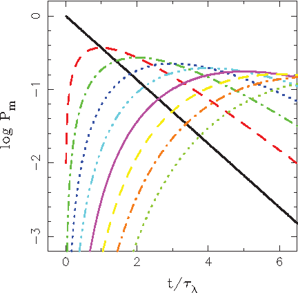
The Poissonian probabilities calculated using Equation (5) are shown in Figure 1 as a family of lines representing probabilities of occurrence of m mutations in the sample at a given time. Time is expressed in units of t/τ_λ , where the average interval between two mutations is obtained as τ_λ = 1 /λ .

OPEN IN VIEWER

FIG. 1.

Probabilities of occurrence of m mutations in a sample at a given time. Lines represent probabilities P_m calculated for m  = 0−8 using Equation (5).

One easily recognizes the dependence for m =0 (see Equation (1)): an exponential that is represented by a straight line on the logarithmic scale. Other lines follow, for increasing values of m , and peak correspondingly at time t/τ_λ  =  m .

Since the most characteristic property of biological systems is their fast growth under favorable conditions, it is worthwhile to note that while, for simplicity, the model was formulated for a population with constant total number of haplotypes, it can be easily modified for exponential growth even with time-dependent growth rate, and the resulting Poissonian distribution (5) will remain unchanged when the analogue of the expression for N_m ( t ) in Equation (4) is normalized by the total number of haplotypes at a given time.

3. Test with Data

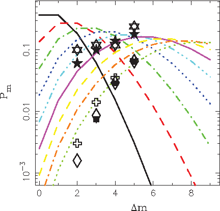
A test was performed with a single Y-DNA haplotype (originating in Slovakia, haplogroup determined as R1b), which is represented by a number of repetitions of nucleotide sequences in 17 specific locations on the Y-chromosome (STR markers). Using this haplotype (referred to as haplotype A ), a search for haplotypes distanced by Δ m mutations was performed using the database Ysearch.org which contains around 90,000 individual records. The distributions of discovered haplotypes with specific mutation distances integrated over the 17 STR markers are shown in Figure 2.

OPEN IN VIEWER

FIG. 2.

Distribution of mutation distances. Lines are the distributions calculated using Equation (5) for constant time step τ_λ . Five- and six-pointed asterisks are haplotypes from Slavic countries, distanced from haplotypes A and B by Δ m mutations, found in database Ysearch.org, Diamonds and squares are all haplotypes, distanced from the haplotype A by Δ m mutations, found in databases Ysearch.org and Ybase.org, Crosses are all haplotypes, distanced from the haplotype B by Δ m mutations, found in the database Ysearch.org.

Lines represent the Poissonian distributions expressed by Equation (5), for a given number of mutations, at times increasing by a constant step of τ_λ . The five-pointed asterisks represent the number of occurrences of haplotypes with a given mutation distance Δ m , originating from the Slavic countries, while diamonds represent the number of occurrences without geographical restrictions, dominant haplotypes from the British Isles (mostly from Scotland and Ireland) and the United States. Squares represent the number of occurrences without geographical restrictions, obtained using an alternative database, Ybase.org again dominated by haplotypes from the British Isles and the United States.

It appears that the results for the Slavic countries represent a lower mean number of mutations compared to the results without geographical restrictions, however, more detailed analysis is difficult due to uncertainty in selection of proper normalization of incomplete distributions, which can be convolutions of several components. The comparison of results obtained using different databases shows consistent agreement, demonstrating reproducibility of the procedure.

For reference, an analogous search was performed for a haplotype with mutation distance Δ m  = 1, discovered in the database YHRD.org in six records distributed in countries with a Slavic population (further referred to as haplotype B ). Results of a search using the database Ysearch.org are shown for the Slavic countries and without geographical restrictions, as six-pointed asterisks and crosses, respectively. Comparison with the searches, performed using the haplotype A , indicates shorter mean mutation distance; however, it is difficult to make unambiguous quantitative conclusions without proper normalization.

4. Probability Ratios and Hyperbolic Scaling

The situation in Figure 2 illustrates how difficult it is to make quantitative conclusions without proper normalization, due to incomplete mutation distributions and possible convolution of several components. The situation is quite similar to investigations of nuclear reactions, in which reconstructed distributions of observables represent convolutions of collisions at various impact parameters evolving by different reaction mechanisms on various time scales. One possibility to circumvent these difficulties is to use relative observables, such as yield ratios, between yields of various reaction products in a given reaction or between yields of identical products in two different reactions. An overview of methods can be found in Veselsky (2005).

In the present case, one can attempt to introduce a procedure, based on relative observables analogous to yield ratios in nuclear processes. As a starting point, Equation (5) can be used to calculate the ratios of Poissonian probabilities for m  + 1 and m mutations at a given time t , \documentclass{aastex}\usepackage{amsbsy}\usepackage{amsfonts}\usepackage{amssymb}\usepackage{bm}\usepackage{mathrsfs}\usepackage{pifont}\usepackage{stmaryrd}\usepackage{textcomp}\usepackage{portland, xspace}\usepackage{amsmath, amsxtra}\pagestyle{empty}\DeclareMathSizes{10}{9}{7}{6}\begin{document}\begin{align*}\frac{\textbf{\textit{P}}_{\textbf{\textit{m} + 1}} (\textbf{\textit{t}})}{\textbf{\textit{P}}_{\textbf{\textit{m}} (\textbf{\textit{t}})}} = \frac{\lambda \textbf{\textit{t}}}{\textbf{\textit{m} + 1}} = \frac{\frac{\textbf{\textit{t}}}{\tau \lambda}}{\textbf{\textit{m} + 1}} \tag{6}\end{align*}\end{document}

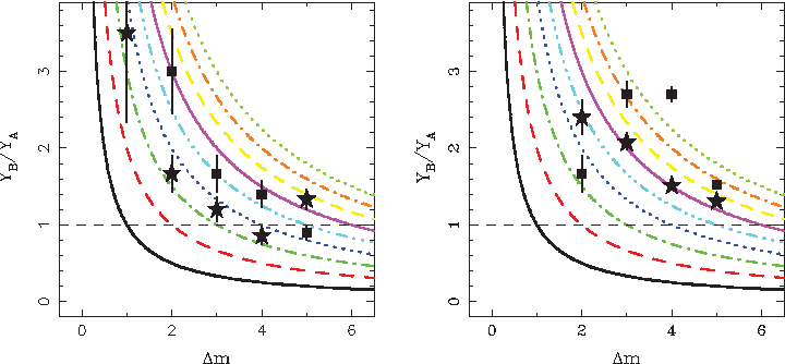
which leads to characteristic hyperbolic time dependences as shown in Figure 3 by a set of lines. Such dependences reflect evolution of mutation distance distributions in an independent system starting from a single haplotype, described by Equations (1) through (5), for a constant time step τ_λ . In principle, one could also consider inverted ratios, leading to straight lines with decreasing slopes; nevertheless, the representation via hyperbolas is more sensitive, especially for smaller samples and mutation distances.

OPEN IN VIEWER

FIG. 3.

The left panel shows ratios of numbers of haplotypes with a given mutation distance Δ m for pairs of haplotypes A − B (asterisks) and C − A (squares) found in the search restricted to Slavic countries. Lines represent calculated probability ratios P_m / P_{m +1} for m  = 0−8, expressed as a function of the mean number of mutations. The right panel shows similar content as the left panel except that the search is without geographical restrictions.

A corresponding test with data can be performed by calculating ratios of mutation distance distributions, shown in Figure 2, obtained for a pair of haplotypes A and B , which differ by one mutation. The resulting dependences can be compared to model values calculated using Equation (6), the difficulties with proper normalization can thus be solved. This again is reminiscent of procedures often employed in nuclear physics, where conditions at specific stages of nuclear multi-fragmentation, or relativistic nucleus–nucleus collisions at the large hadron collider (LHC), are reconstructed from final observables using the appropriate model assumptions. The results of the procedure in the present case are shown in Figure 3. In the left panel of Figure 3, the asterisks represent the results for haplotypes A and B within Slavic countries. The squares represent analogous results for a pair of haplotypes, where the haplotype A is compared to the only other haplotype with mutation distance Δ m  = 1, found in the database YHRD.org in one record (further referred to as C ).

It is apparent that both dependences assume the expected hyperbolic shapes and thus represent the behavior described by the model presented above. Specifically, such hyperbolic scaling of the ratios P _{m +1} ( t ) /P_m ( t ) means that these ratios are consistent with evolution from a single haplotype in an independent system. The dependence for the haplotype pair A − B is located between two hyperbolas representing the times 3 and 4 τ_λ , except for the last point, which will be discussed later. This indicates that within a given R1b population, the two haplotypes are at the initial stage of the haplotype tree, which evolves independently during a time 3−4 τ_λ since the moment when the haplotype A emerged, or eventually when the population carrying this haplotype split from larger R1b population as a result of migration. If the order of mutations were opposite, the dependence would assume a corresponding straight line. The dependence for the haplotype pair C − A is located close to the hyperbola representing the evolution time 5 τ_λ , and it can be considered as representing the mutation preceding the mutation represented by the haplotype pair A − B . The difference of the two “experimental” hyperbolas appears to be 50% larger than the mean time gap between mutations, however, one has to keep in mind that mutation is a stochastic process, and thus it does not happen at equal time intervals.

On the right panel of Figure 3, asterisks again represent the results for the haplotype pair A − B , while squares represent the results for the haplotype pair C − A ; however, in this case the search is carried out without geographical restrictions (dominated by haplotypes from the British Isles). Interestingly, in this case the dependence for the haplotype pair A − B is consistent with a hyperbola representing the evolution time 6 τ_λ , and it appears that the common ancestor of haplotypes found without geographical restrictions is older than the common ancestor of haplotypes found in searches restricted to Slavic countries by 2−3 τ_λ . This can be caused by admixture from the descendants of haplotypes closely related to haplotypes A − B , which at mutation distances Δ m  = 3 start to dominate the trend, as documented by the breakdown of the hyperbolic dependence without geographic restrictions at Δ m  = 2, where haplotypes from the British Isles are not dominant. Thus, the common ancestor found at 6 τ_λ is not necessarily the haplotype pair A − B but some related haplotype, differing by one mutation step early in the sequence, which evolved separately, most likely in Western Europe.

Reciprocally, the dependence for the haplotype pair A − B obtained without geographical restrictions also appears to explain the fact that in the search restricted to Slavic countries, hyperbolic scaling breaks down at Δ m  = 5. Apparently, at this mutation distance the ratio reverts to the trend obtained in the search without geographical restrictions shown in the right panel.

The dependence for the haplotype pair C − A , obtained without geographical restrictions (squares), does not exhibit a hyperbolic shape, instead it appears to initially grow. One can consider it as a mixture of its descendant haplotypes and descendants of preceding or contemporary haplotypes, as one would expect if the haplotype C was close to the center of the haplotype distribution at the time of its emergence and separation from the rest of the population. Thus, the haplotype C appears to be an R1b haplotype, transferred by migration or emerging just thereafter and admixed into the Slavic population, of which the haplotypes A and B appear to be subsequent descendants.

Using the literature (Gusmao et al., 2005) and assuming an interval of 30 years per generation, the value of τ_λ can be estimated at approximately 830 years, so the time of independent evolution of the sequence of R1b haplotypes starting with the haplotype C among the predecessors of contemporary Slavs, determined as 5 τ_λ , can be estimated at 4,150 years, with an uncertainty of about 400 years (0.5 τ_λ ). Furthermore, the age of the common ancestor of all considered R1b haplotypes within European population, determined as 6 τ_λ , can be estimated as 5,000 years, again with an uncertainty of about 400 years.

Since the available data are dominated by haplotypes from the British Isles, one can try further analysis of this sample by selecting pairs of subsequent haplotypes from this area. Two such pairs were identified among the results of the searches performed using the haplotypes A − C , the first one represented by the records N43KH and GXD83, and the second one by YNGCV and SAHFV. Both pairs are relatively less frequent within the European R1b populations and thus may be rather old.

The left panel of Figure 4 shows ratios of numbers of haplotypes with a given mutation distance Δ m for these two pairs of haplotypes (squares and asterisks, respectively) found in the nonrestricted search at Ysearch.org, and one can see a similar situation to the right panel of Figure 3. The pair represented by asterisks appears to represent a similar age to the common ancestor found in the search with pair of haplotypes A and B (5,000 years), while the other pair appears younger by approximately 2 τ_λ , which results in 3,300 years of age. Thus, there can be some age structure in this population, possibly as a result of subsequent waves of migrations into the British Isles. This possibility may be reflected by a structure of the haplotype distribution. A relatively distant haplotype from outside of the contemporary haplotype distribution can serve as a probe and possibly reveal such structure.

OPEN IN VIEWER

FIG. 4.

Left panel: Ratios of numbers of haplotypes with a given mutation distance Δ m for two Δ m  = 1 pairs of haplotypes from the British Isles (asterisks and squares) found in the nonrestricted search at Ysearch.org, Lines represent calculated probability ratios P_m / P_{m +1} for m  = 0−8, expressed as a function of the mean number of mutations. Right panel: Squares represent numbers of haplotypes, distanced from haplotype C by Δ m mutations, found at Ysearch.org, Lines represent calculated distributions.

Squares in the right panel of Figure 4 show a distribution of mutation distances from a rather old haplotype C , obtained from a search on the Ysearch.org database. Comparison with shapes of calculated distributions (lines) appears to demonstrate that the mutation distance distribution may be a convolution of at least two components with unequal total weights, of which the younger (more distant) one appears to dominate. This could also explain irregularity in the hyperbolic dependence represented by asterisks in the left panel of Figure 4, since the left part of the dependence is apparently older and possibly further from the center of contemporary haplotype distribution.

Based on the above analysis, one can also try to investigate available R1b haplotypes, attributed to historical persons. Figure 5 shows ratios of numbers of haplotypes with a given mutation distance Δ m from two Δ m  = 1 pairs of R1b haplotypes, found in a nonrestricted search on Ysearch.org. One haplotype of each pair belongs to historical persons, Nikolai II Romanov and Tutankhamen (squares and asterisks).

OPEN IN VIEWER

FIG. 5.

Ratios of numbers of haplotypes with a given mutation distance Δ m from two Δ m  = 1 pairs of R1b haplotypes, found in a nonrestricted search on Ysearch.org. One haplotype of each pair belongs to historical persons, Nikolai II Romanov and Tutankhamen (squares and asterisks). Lines represent calculated probability ratios P_m / P_{m +1} for m  = 0−9, expressed as a function of the mean number of mutations.

The haplotype of Nikolai II Romanov (GXK2B) is complemented by a nearest haplotype from a person of Russian origin, apparently a member of the Romanov family (7UFPX). The resulting dependence, obtained for this pair in a geographically unrestricted search (dominated by haplotypes from Western Europe), is close to the one obtained using the younger of the two haplotype pairs from British Isles (squares in the right panel of Figure 4), and thus the age of the pair of haplotypes within the population of Western Europe can be estimated to be 3,300 years. This is indeed consistent with a German origin of the male line of the Romanov family, since the 18th century.

Since the haplotype of Tutankhamen (ER7RQ) is rather distant from the distribution of existing R1b haplotypes in the database, it was complemented by a haplotype claimed to belong to remains found in an archaeological location in Lebanon, which is mentioned in the supplementary commentary to the record in the Ysearch.org database. The position in Figure 5 apparently means that a common ancestor with the related haplotypes in the distribution of European R1b lived before 8−9 τ_λ (6500–7500 years), which might be the time when the ancestors of Tutankhamen split from the ancestors of the population that now lives in Europe. Obviously, to claim that the haplotype of Tutankhamen is the haplotype of the common ancestor would be rather far-reaching since data at smaller mutation distances are missing, and thus an accidental, later, and closer approach of branches in the mutation tree cannot be excluded. A larger systematic of R1b haplotypes from the Middle East would be helpful for further analyses.

Concerning the method presented here, analogy of DNA mutation to radioactive decay and chemical kinetics was employed already by Klyosov (2009). His method uses Equation (1) to determine the age of the common ancestor of the whole sample of haplotypes. This is achieved by comparison of the total number of haplotypes in the sample to the number of mutations within the sample, which is obtained by constructing detailed mutation trees for the whole sample. In a mathematical sense, such a method relies on integral observables, while the method presented here uses differential observables and can relate individual haplotypes to the bulk of the haplotype distribution or its subparts. Ultimately, both methods are complementary.

Klyosov (2010), after applying his method separately to R1b populations in various countries, arrives at the conclusion that, on its migration to Europe, the R1b population split once, about 6,000 years ago in the territory of Asia Minor. Its final expansion into the whole of Western and Central Europe, and its separation into local populations, occurred around 4,000 years ago, during expansion of the archaeological Bell Beaker culture. These times of migrations, resulting in the splitting of the R1b population, are, in principle, consistent with the results obtained in the present work. Both methods thus appear to be in mutual agreement.

The method presented in this work is specific in its capability to perform quick age estimates for individual haplotypes. It is suitable specifically for unique haplotypes away from the center of haplotype distributions, while for more common haplotypes proper choice of the Δ m  = 1 haplotype will be necessary.

Klyosov (2009) mentions occurrence of reverse mutations, which influence the mutation counting and thus distort the final time estimate. The model, presented in this article, relies on comparison of observables of subsequent mutation stages, and the results cannot be dramatically influenced by this circumstance. One can still introduce a minor correction in the form of a reduced mutation rate. For a set of 17 STR markers, such correction will be less than 2% per generation.

In summary, the method, inspired by analogous procedures used in the physics of nuclear multi-fragmentation, allows for an established order of precedence, and determine age of pairs of haplotypes separated by one mutation. For both haplotypes of the pair, searches for existing haplotypes, differing by increasing numbers of mutations, are carried out using a haplotype database. The resulting ratios of frequencies of haplotypes, found at given mutation distances, are compared to calculated probability ratios. The order of precedence and age of the pair of haplotypes can be deduced when resulting ratios follow a hyperbolic dependence. The method provides a simple tool that can be used with relatively small and not necessarily complete samples, available in publicly accessible databases.