Identifying Complexes from Protein Interaction Networks According to Different Types of Neighborhood Density

Abstract

To facilitate the realization of biological functions, proteins are often organized into complexes. While computational techniques are used to predict these complexes, detailed understanding of their organization remains inadequate. Apart from complexes that reside in very dense regions of a protein interaction network in which most algorithms are able to identify, we observe that many other complexes, while not residing in very dense regions, reside in regions with low neighborhood density. We develop an algorithm for identifying protein complexes by considering these two types of complexes separately. We test our algorithm on a few yeast protein interaction networks, and show that our algorithm is able to identify complexes more accurately than existing algorithms. A software program NDComplex for implementing the algorithm is available at http://faculty.cse.tamu.edu/shsze/ndcomplex.

1. Introduction

Since experimental determination of protein complexes remains difficult, computational techniques are used to predict protein complexes. While a common strategy is to predict complexes from given protein interaction networks (Bader and Hogue, 2003; King et al., 2004; Sharan et al., 2005; Altaf-Ul-Amin et al., 2006; Hirsh and Sharan, 2007; Li et al., 2007; Chua et al., 2008; Qi et al., 2008; Liu et al., 2009; Moschopoulos et al., 2009; Jung et al., 2010; Shi et al., 2011; Tu et al., 2011), recent combined experimental–computational strategies utilize these techniques to construct protein complexes from purification data (Gavin et al., 2002; Ho et al., 2002; Krogan et al., 2006).

Apart from the general agreement that protein complexes form dense subgraphs in an interaction network (Spirin and Mirny, 2003), which leads to the strategy of first generating small dense subgraphs and either extending or merging these subgraphs to construct protein complexes (Bader and Hogue, 2003; Li et al., 2007), detailed understanding of the organization of protein complexes remains inadequate. To improve the modeling of complexes, recent approaches separate the tasks of predicting a core complex and its attachment proteins (Leung et al., 2009; Wu et al., 2009).

We observe that most complexes either reside in very dense regions, in which most algorithms are able to identify, or they reside in regions with low neighborhood density, in which most algorithms are less successful to identify. We investigate the following algorithm to consider these two types of complexes separately. Given a protein interaction network, we first identify all the maximal cliques. For each maximal clique, we count the number of other maximal cliques that overlap significantly with it and use it to define neighborhood density. We subdivide these cliques into two sets, with one containing cliques with low neighborhood density and the other containing cliques with high neighborhood density.

Since the maximal cliques with low neighborhood density are likely to correspond to the core region of a complex, we extend each clique to include more proteins as long as the density remains high. This allows each prediction to become a dense subgraph that is not necessarily a clique. Since the maximal cliques with high neighborhood density have overlap with many other maximal cliques, using these cliques directly, as predicted complexes, will lead to significant overestimate of the number of complexes. We extract the most shared sets of proteins from these cliques. We obtain the set of predicted complexes by collecting the above two types of predictions.

We compare the performance of our algorithm to other complex prediction algorithms on a few protein interaction networks and show that our algorithm is able to identify complexes more accurately with respect to complex agreement, complex accuracy, and protein pair agreement measures.

2. Methods

2.1. Neighborhood density

Given a protein interaction network represented by a graph G=(V, E), in which each vertex represents a protein and each edge represents interaction between two proteins, we first obtain the set \documentclass{aastex}\usepackage{amsbsy}\usepackage{amsfonts}\usepackage{amssymb}\usepackage{bm}\usepackage{mathrsfs}\usepackage{pifont}\usepackage{stmaryrd}\usepackage{textcomp}\usepackage{portland, xspace}\usepackage{amsmath, amsxtra}\pagestyle{empty}\DeclareMathSizes{10}{9}{7}{6}\begin{document} $${ \cal C}$$\end{document} of all maximal cliques with at least three vertices by using a branch-and-bound algorithm to add one vertex at a time until no more vertices can be added. Since the degree of most vertices in G is small, the number of maximal cliques is not large and this step is feasible, with time complexity \documentclass{aastex}\usepackage{amsbsy}\usepackage{amsfonts}\usepackage{amssymb}\usepackage{bm}\usepackage{mathrsfs}\usepackage{pifont}\usepackage{stmaryrd}\usepackage{textcomp}\usepackage{portland, xspace}\usepackage{amsmath, amsxtra}\pagestyle{empty}\DeclareMathSizes{10}{9}{7}{6}\begin{document} $$O ( \mid { \cal C} \mid \mid V \mid ^2 )$$\end{document} .

Given two sets C₁ and C₂, we define their similarity to be S(C₁, C₂)=|C₁ ∩ C₂|²/(|C₁||C₂|) (Bader and Hogue, 2003; Altaf-Ul-Amin et al., 2006; Li et al., 2007; Chua et al., 2008; Moschopoulos et al., 2009; Wu et al., 2009; Jung et al., 2010; Shi et al., 2011). For each maximal clique C, we count the number of other maximal cliques C′ with S(C, C′)≥t, where t is a given threshold. We define a clique C to have low neighborhood density if this number is below a given threshold c, and it has high neighborhood density otherwise. The worst case time complexity of this step is \documentclass{aastex}\usepackage{amsbsy}\usepackage{amsfonts}\usepackage{amssymb}\usepackage{bm}\usepackage{mathrsfs}\usepackage{pifont}\usepackage{stmaryrd}\usepackage{textcomp}\usepackage{portland, xspace}\usepackage{amsmath, amsxtra}\pagestyle{empty}\DeclareMathSizes{10}{9}{7}{6}\begin{document} $$O ( \mid { \cal C} \mid ^2 \mid V \mid ).$$\end{document}

2.2. Cliques with low neighborhood density

Given an induced subgraph G′=(V′, E′) of a graph G=(V, E), we define its density to be D(V′)=2|E′|/(|V′|(|V′|−1)) (Bader and Hogue, 2003; Altaf-Ul-Amin et al., 2006; Li et al., 2007; Moschopoulos et al., 2009; Wu et al., 2009; Shi et al., 2011). For each maximal clique with low neighborhood density, we iteratively identify the best vertex to add so that the density of the enlarged subgraph remains high and the length of the shortest path between two vertices in the enlarged subgraph remains small. We repeat the procedure until no more changes can be made, and use the resulting dense subgraphs as predicted complexes (Fig. 1). Since these subgraphs reside in regions with low neighborhood density, they are likely to function as an independent unit.

FIG. 1.

Algorithm NDComplexL is used to obtain predicted complexes from maximal cliques with low neighborhood density.

For each potential vertex to add, it takes O(|V|) time to compute the density of the enlarged subgraph. By precomputing all vertex pairs that have shortest paths of length at most two, the worst case time complexity of the procedure is \documentclass{aastex}\usepackage{amsbsy}\usepackage{amsfonts}\usepackage{amssymb}\usepackage{bm}\usepackage{mathrsfs}\usepackage{pifont}\usepackage{stmaryrd}\usepackage{textcomp}\usepackage{portland, xspace}\usepackage{amsmath, amsxtra}\pagestyle{empty}\DeclareMathSizes{10}{9}{7}{6}\begin{document} $$O ( \mid { \cal C} \mid \mid V \mid^2)$$\end{document} , although it should terminate quickly when the density threshold is large.

2.3. Cliques with high neighborhood density

For each maximal clique with high neighborhood density, if its most similar maximal clique overlaps significantly with it, we replace it by the intersection of the two cliques. We repeat the procedure until no more changes can be made, and use the remaining cliques as predicted complexes (Fig. 2). This procedure reduces the number of highly overlapping predictions significantly, since many cliques become identical after the intersections.

FIG. 2.

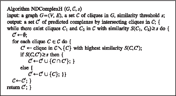
Algorithm NDComplexH is used to obtain predicted complexes from maximal cliques with high neighborhood density.

By labeling each clique with a positive integer and picking the one with the lowest label when resolving ties in similarity, we can guarantee that at least two cliques become identical after each iteration, and the procedure takes at most \documentclass{aastex}\usepackage{amsbsy}\usepackage{amsfonts}\usepackage{amssymb}\usepackage{bm}\usepackage{mathrsfs}\usepackage{pifont}\usepackage{stmaryrd}\usepackage{textcomp}\usepackage{portland, xspace}\usepackage{amsmath, amsxtra}\pagestyle{empty}\DeclareMathSizes{10}{9}{7}{6}\begin{document} $$\mid { \cal C} \mid$$\end{document} iterations. The worst case time complexity of the procedure is \documentclass{aastex}\usepackage{amsbsy}\usepackage{amsfonts}\usepackage{amssymb}\usepackage{bm}\usepackage{mathrsfs}\usepackage{pifont}\usepackage{stmaryrd}\usepackage{textcomp}\usepackage{portland, xspace}\usepackage{amsmath, amsxtra}\pagestyle{empty}\DeclareMathSizes{10}{9}{7}{6}\begin{document} $$O(\mid {\cal C} \mid^3 \mid V \mid)$$\end{document} , although it should terminate quickly when the similarity threshold is large.

3. Results

3.1. Performance evaluation

We use a combined set of true complexes that contain at least two proteins to which we compare the predicted complexes, including 214 curated complexes from the Munich Information Center for Protein Sequences (MIPS) database (Mewes et al., 2004), 101 curated complexes from Aloy et al. (2004), and 363 complexes extracted from the Saccharomyces Genome Database (SGD; Cherry et al., 1998), according to GO slim complex annotations (Friedel et al., 2009). To reduce evaluation bias, we have removed complexes that contain more than 100 proteins from the SGD complexes. We removed the duplicates from the combined set, resulting in a total of 574 true complexes. Most of these complexes are small, with the average number of proteins within a complex being 9.4 (Table 1).

Table 1.

Distribution of True Complexes Used in the Evaluation

Protein	Complex	Protein	Complex	Protein	Complex
2	116	5	47	8	24
3	96	6	32	9	13
4	67	7	32	≥10	147

Complex denotes the number of complexes that have number of proteins specified by Protein.

We used the yeast protein interaction network from the MIPS database (Mewes et al., 2004), the yeast protein interaction network from the Database of Interacting Proteins (DIP database) (Xenarios et al., 2000), and the yeast protein interaction network from the Biological General Repository for Interaction Datasets (BioGRID database) (Stark et al., 2006) to obtain separate sets of predicted complexes from each network. For the BioGRID network, only physical interactions are included. These networks have different densities, with the BioGRID network being the densest (Table 2).

Table 2.

Protein Interaction Networks Used in the Evaluation

	Protein	Interaction	Avg_deg	Max_deg	Density
MIPS	4546	12319	5.4	286	0.0012
DIP	4945	21639	8.8	281	0.0018
BioGRID	5727	51319	17.9	2553	0.0031

Protein, interaction, avg_deg, max_deg, and density denote the number of proteins, the number of interactions, the average vertex degree, the maximum vertex degree, and the density of the network, respectively.

3.2. Performance comparisons

We compared the performance of our algorithm NDComplex to the Markov cluster algorithm (MCL) (Enright et al., 2002), which subdivides a given graph into clusters by Markov clustering, to the Molecular complex detection algorithm (MCODE) (Bader and Hogue, 2003), which uses a seed-extension algorithm to identify complexes in dense regions, to the Dense-neighborhood extraction using connectivity and confidence features algorithm (DECAFF) (Li et al., 2007), which is based on the identification and merging of dense subgraphs, and to the Core-attachment based method (COACH) (Wu et al., 2009), which is based on the prediction of a core complex and its attachment proteins. We also compared the performance of our algorithm to the Maximal clique algorithm (CLIQUE), which uses the set of maximal cliques with at least three vertices as predicted complexes.

For MCL, we set inflation to 3.5. For MCODE, we set depth to 100, haircut to true, fluff to false, and fluff density threshold to 0.2. For DECAFF, we implement steps 1 to 4 of Algorithm 1 in Li et al. (2007), including the local clique detection step, the hub removal step, and the merging step, and set the density threshold to 0.8 and the neighborhood affinity threshold to 0.5. Since the other algorithms do not use functional information, we skip the filtering steps 5 to 9 in DECAFF that use the MIPS functional catalog (Mewes et al., 2004). For COACH, we set the neighborhood affinity threshold to 0.1. For NDComplex, we set the similarity threshold t and the occurrence threshold c during the computation of neighborhood density to 0.3 and 3 respectively. We set the density threshold d to 0.7 during the computation of predicted complexes in regions with low neighborhood density, and the similarity threshold s to 0.2 during the computation of predicted complexes in regions with high neighborhood density. These parameters are determined by testing a few combinations and choosing the one that gives the best overall performance on the test sets. We collect the predicted complexes from both types of regions for performance evaluation, with each distinct prediction counted once.

3.3. Complex agreement measure

Given a similarity threshold u, we evaluate the agreement between a set of true complexes and a set of predicted complexes by defining the precision (PC) to be the ratio of the number of predicted complexes P that have a true complex C with similarity S(C,P)≥u to the total number of predicted complexes, and the recall (RC) to be the ratio of the number of true complexes C that have a predicted complex P with similarity S(C, P)≥u to the total number of true complexes (Chua et al., 2008; Moschopoulos et al., 2009; Wu et al., 2009; Jung et al., 2010; Shi et al., 2011). We compute the F-measure=2×(PC×RC)/(PC+RC).

Figure 3 shows that NDComplex has the best overall performance when the similarity threshold u is low, while MCODE and COACH perform better when the similarity threshold u is high, which corresponds to a small number of almost perfect predictions. DECAFF has the next best performance, followed by CLIQUE and MCL.

FIG. 3.

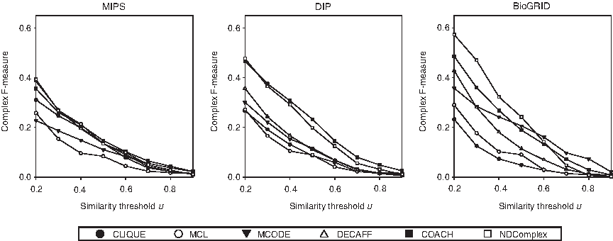
Performance of complex prediction algorithms on each protein interaction network with respect to the complex agreement measure over different similarity thresholds u between a true complex and a predicted complex. For DECAFF, only steps 1 to 4 of Algorithm 1 in Li et al. (2007) are included, while the filtering steps 5 to 9 that are based on the use of functional information are skipped.

3.4. Complex accuracy measure

In addition to using the complex agreement measure, we use the complex accuracy measure in Brohée and van Helden (2006), Friedel et al. (2009), and Tu et al. (2011) that does not rely on the use of a similarity threshold. Given a set of true complexes \documentclass{aastex}\usepackage{amsbsy}\usepackage{amsfonts}\usepackage{amssymb}\usepackage{bm}\usepackage{mathrsfs}\usepackage{pifont}\usepackage{stmaryrd}\usepackage{textcomp}\usepackage{portland, xspace}\usepackage{amsmath, amsxtra}\pagestyle{empty}\DeclareMathSizes{10}{9}{7}{6}\begin{document} $${ \cal C}$$\end{document} and a set of predicted complexes \documentclass{aastex}\usepackage{amsbsy}\usepackage{amsfonts}\usepackage{amssymb}\usepackage{bm}\usepackage{mathrsfs}\usepackage{pifont}\usepackage{stmaryrd}\usepackage{textcomp}\usepackage{portland, xspace}\usepackage{amsmath, amsxtra}\pagestyle{empty}\DeclareMathSizes{10}{9}{7}{6}\begin{document} $${ \cal P}$$\end{document} , we compute the sensitivity \documentclass{aastex}\usepackage{amsbsy}\usepackage{amsfonts}\usepackage{amssymb}\usepackage{bm}\usepackage{mathrsfs}\usepackage{pifont}\usepackage{stmaryrd}\usepackage{textcomp}\usepackage{portland, xspace}\usepackage{amsmath, amsxtra}\pagestyle{empty}\DeclareMathSizes{10}{9}{7}{6}\begin{document} $${ \rm Sn} = \sum\nolimits_{C \in { \cal C}} {\max}_{P \in {\cal P}} \mid C \cap P \mid / \sum\nolimits_{C \in { \cal C}} \mid C \mid$$\end{document} , which is the ratio of the sum of the maximum overlap of each true complex with a predicted complex to the total size of true complexes, the positive predictive value \documentclass{aastex}\usepackage{amsbsy}\usepackage{amsfonts}\usepackage{amssymb}\usepackage{bm}\usepackage{mathrsfs}\usepackage{pifont}\usepackage{stmaryrd}\usepackage{textcomp}\usepackage{portland, xspace}\usepackage{amsmath, amsxtra}\pagestyle{empty}\DeclareMathSizes{10}{9}{7}{6}\begin{document} $${ \rm PPV} = \sum\nolimits_{P \in { \cal P}} {\max}_{C \in { \cal C}} \mid C \cap P \mid / \sum\nolimits_{P \in { \cal P}} \mid P \mid$$\end{document} , which is the ratio of the sum of the maximum overlap of each predicted complex with a true complex to the total size of predicted complexes, and the accuracy \documentclass{aastex}\usepackage{amsbsy}\usepackage{amsfonts}\usepackage{amssymb}\usepackage{bm}\usepackage{mathrsfs}\usepackage{pifont}\usepackage{stmaryrd}\usepackage{textcomp}\usepackage{portland, xspace}\usepackage{amsmath, amsxtra}\pagestyle{empty}\DeclareMathSizes{10}{9}{7}{6}\begin{document} $${ \rm Acc} = \sqrt{{ \rm Sn} \times { \rm PPV}}$$\end{document} , which is the geometric mean of sensitivity and PPV.

Figure 4 shows that NDComplex has the best accuracy in almost all cases, followed by CLIQUE, DECAFF, and COACH. The performance differences between NDComplex and MCL, MCODE, DECAFF, or COACH are the largest on the BioGRID network. DECAFF puts emphasis on sensitivity, while MCODE puts emphasis on PPV.

FIG. 4.

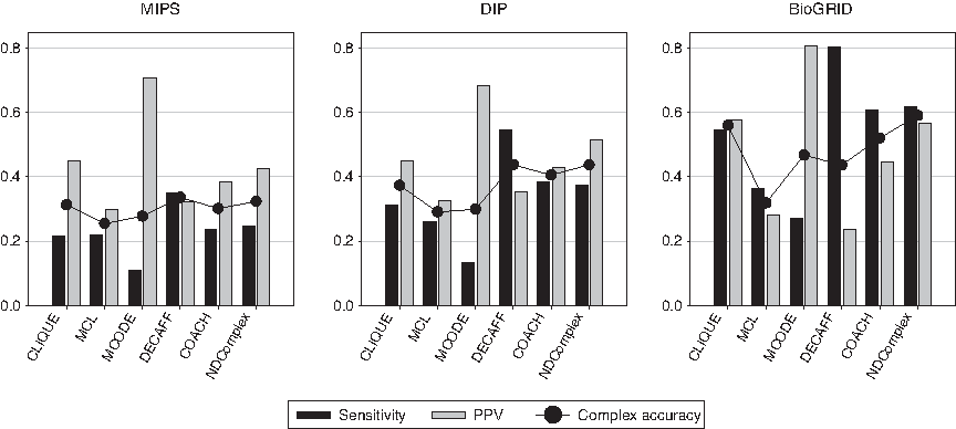
Performance of complex prediction algorithms on each protein interaction network with respect to the complex accuracy measure.

3.5. Protein pair agreement measure

We evaluate the protein pair agreement by defining a true positive (TP) to be a protein pair that is within the same true complex and within the same predicted complex, a false positive (FP) to be a protein pair that is within the same predicted complex but not in the same true complex, and a false negative (FN) to be a protein pair that is within the same true complex but not in the same predicted complex. We compute the precision PC=|TP|/(|TP|+|FP|), the recall RC=|TP|/(|TP|+|FN|), and the F-measure=2×(PC×RC)/(PC+RC).

When the true complexes and the predicted complexes both consist of disjoint sets of proteins, this measure evaluates the resemblance of the two sets. Since a protein can appear in more than one complex, this measure evaluates how accurately an algorithm can predict whether a given pair of proteins are within the same complex or not, although this is only an approximation since the set of true complexes may not be complete.

Figure 5 shows that COACH and NDComplex have the best performance with respect to protein pairs. The performance differences between these algorithms and MCL, MCODE, or DECAFF are especially large on the BioGRID network, with CLIQUE performing better than MCL, MCODE, and DECAFF. MCL and DECAFF have low performance on the BioGRID network due to a large number of false positive protein pairs. MCODE puts emphasis on precision, while DECAFF puts emphasis on recall.

FIG. 5.

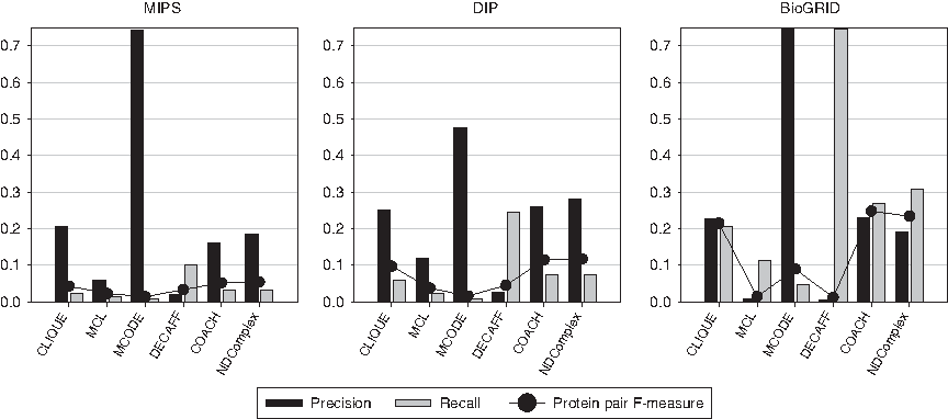
Performance of complex prediction algorithms on each protein interaction network with respect to the protein pair agreement measure.

4. Discussion

We have developed an algorithm to identify complexes from protein interaction networks based on using different strategies for regions with different neighborhood densities. We have shown that this approach is very effective and it achieves the best performance with respect to complex agreement, complex accuracy, and protein pair agreement measures. Among the three networks that we have tested, we found that each algorithm performs the best on the BioGRID network, which has the highest density, with weaker performance on the DIP network, followed by the MIPS network, which has the lowest density. On the BioGRID network, our algorithm NDComplex performs the best with respect to the complex agreement measure when the similarity threshold u is low, and with respect to the complex accuracy measure, while COACH and NDComplex have the best and comparable performance with respect to the protein pair agreement measure.

Ideally, the correspondences between the true complexes and the predicted complexes should be one-to-one. To evaluate the degree of success of each algorithm in reaching this goal, we use the separation measure in Brohée and van Helden (2006) and Tu et al. (2011). Given a true complex C and a predicted complex P, define their separation Sep \documentclass{aastex}\usepackage{amsbsy}\usepackage{amsfonts}\usepackage{amssymb}\usepackage{bm}\usepackage{mathrsfs}\usepackage{pifont}\usepackage{stmaryrd}\usepackage{textcomp}\usepackage{portland, xspace}\usepackage{amsmath, amsxtra}\pagestyle{empty}\DeclareMathSizes{10}{9}{7}{6}\begin{document} $$( C , P ) = \mid C \cap P \mid ^2 / ( \sum\nolimits_{C \in { \cal C}} \mid C \cap P \mid \sum\nolimits_{P \in { \cal P}} \mid C \cap P \mid)$$\end{document} . Given a set of true complexes \documentclass{aastex}\usepackage{amsbsy}\usepackage{amsfonts}\usepackage{amssymb}\usepackage{bm}\usepackage{mathrsfs}\usepackage{pifont}\usepackage{stmaryrd}\usepackage{textcomp}\usepackage{portland, xspace}\usepackage{amsmath, amsxtra}\pagestyle{empty}\DeclareMathSizes{10}{9}{7}{6}\begin{document} $${ \cal C}$$\end{document} and a set of predicted complexes \documentclass{aastex}\usepackage{amsbsy}\usepackage{amsfonts}\usepackage{amssymb}\usepackage{bm}\usepackage{mathrsfs}\usepackage{pifont}\usepackage{stmaryrd}\usepackage{textcomp}\usepackage{portland, xspace}\usepackage{amsmath, amsxtra}\pagestyle{empty}\DeclareMathSizes{10}{9}{7}{6}\begin{document} $${ \cal P}$$\end{document} , we compute the average separation over the set of true complexes \documentclass{aastex}\usepackage{amsbsy}\usepackage{amsfonts}\usepackage{amssymb}\usepackage{bm}\usepackage{mathrsfs}\usepackage{pifont}\usepackage{stmaryrd}\usepackage{textcomp}\usepackage{portland, xspace}\usepackage{amsmath, amsxtra}\pagestyle{empty}\DeclareMathSizes{10}{9}{7}{6}\begin{document} $${ \rm Sep \_c} = \sum\nolimits_{C \in { \cal C}} \sum\nolimits_{P \in { \cal P}}{ \rm Sep} ( C , P ) / \mid { \cal C} \mid$$\end{document} , the average separation over the set of predicted complexes \documentclass{aastex}\usepackage{amsbsy}\usepackage{amsfonts}\usepackage{amssymb}\usepackage{bm}\usepackage{mathrsfs}\usepackage{pifont}\usepackage{stmaryrd}\usepackage{textcomp}\usepackage{portland, xspace}\usepackage{amsmath, amsxtra}\pagestyle{empty}\DeclareMathSizes{10}{9}{7}{6}\begin{document} $${ \rm Sep \_p} = \sum\nolimits_{C \in { \cal C}} \sum\nolimits_{P \in { \cal P}}{ \rm Sep} ( C , P ) / \mid { \cal P} \mid$$\end{document} , and the separation \documentclass{aastex}\usepackage{amsbsy}\usepackage{amsfonts}\usepackage{amssymb}\usepackage{bm}\usepackage{mathrsfs}\usepackage{pifont}\usepackage{stmaryrd}\usepackage{textcomp}\usepackage{portland, xspace}\usepackage{amsmath, amsxtra}\pagestyle{empty}\DeclareMathSizes{10}{9}{7}{6}\begin{document} $${ \rm Sep} = \sqrt{{ \rm Sep \_c} \times { \rm Sep \_p}}$$\end{document} , which is the geometric mean of the above two averages.

Table 3 shows that while MCODE has the highest separation, it produces a small number of predictions that cover very few proteins. MCL achieves the next highest separation, but it produces a disjoint partition of proteins, which is biologically inaccurate since it does not allow a protein to appear in multiple predicted complexes. COACH achieves a better separation than NDComplex, but it covers less proteins. CLIQUE and DECAFF cover the most interactions, but the number of predictions is very high and they have the worst separation. NDComplex achieves better separation than CLIQUE and DECAFF.

Table 3.

Statistics of Predicted Complexes from Each Algorithm on Each Protein Interaction Network

	MIPS						DIP						BioGRID
	CLIQUE	MCL	MCODE	DECAFF	COACH	NDComplex	CLIQUE	MCL	MCODE	DECAFF	COACH	NDComplex	CLIQUE	MCL	MCODE	DECAFF	COACH	NDComplex
Complex	2869	1740	57	5328	280	621	7129	2226	52	11434	467	1180	34383	2213	76	35048	672	2600
Protein	1387	4546	233	3550	1024	1144	2161	4945	265	4433	1530	1800	4429	5727	553	5707	2675	3217
Interaction	5648	3051	459	9364	3692	4016	11498	2971	489	18623	6392	7193	42980	6466	2344	49899	22663	27101
Separation	0.0055	0.034	0.046	0.0012	0.029	0.014	0.003	0.033	0.046	0.0006	0.025	0.011	0.0009	0.028	0.051	0.000079	0.016	0.0055

Complex denotes the number of predicted complexes; protein and interaction denote the number of proteins and interactions covered by these complexes, respectively, in the network; and separation denotes the separation between the set of true complexes and the set of predicted complexes.

Table 4 shows the statistics of maximal cliques and predicted complexes during different stages of our algorithm NDComplex. Within each network, the number of maximal cliques with high neighborhood density is much larger than the number of maximal cliques with low neighborhood density, which means that there are significant overlaps among the maximal cliques with high neighborhood density. For regions with low neighborhood density, our strategy can add a large number of proteins to a prediction, which is especially evident on the BioGRID network. While the density of these predictions remains high, the number of predictions decreases since some of them become identical after the addition of proteins. The situation is very different for regions with high neighborhood density, when the number of predictions decreases drastically after the intersections of cliques, and each of these predictions contains a very small number of proteins, which means that there are only a small number of highly shared parts within these cliques. The predictions from these two types of regions are distinct (compare to Table 3), with almost all predictions coming from regions with low neighborhood density. Since this is sufficient to ensure that the predictions have high quality, a complex can be modeled mostly as an independent unit with dense inside connections and sparse outside connections, while the small number of predictions from very dense regions are still needed to reduce false negatives.

Table 4.

Statistics of Maximal Cliques and Predicted Complexes During Different Stages of Our Algorithm NDComplex on Each Protein Interaction Network

	MIPS				DIP				BioGRID
	clique_l	clique_h	complex_l	complex_h	clique_l	clique_h	complex_l	complex_h	clique_l	clique_h	complex_l	complex_h
Number	735	2134	595	26	1333	5796	1159	21	2715	31668	2554	46
Avg_pro	3.2	4.7	8.1	2.5	3.2	3.7	6.6	2.5	3.3	7.7	19.0	2.8
Max_pro	14	12	27	4	9	10	22	4	10	33	80	7

Clique_l and complex_l denote cliques with low neighborhood density and predicted complexes from these cliques, respectively; and clique_h and complex_h denote cliques with high neighborhood density and predicted complexes from these cliques, respectively. In each case, number denotes the total number of cliques or predicted complexes, and avg_pro and max_pro denote the average and maximum number of proteins within a clique or a predicted complex, respectively.

Although the worst case time complexity of our algorithm NDComplex is high, the actual running time is not high (Table 5). For sparse networks such as MIPS and DIP, it takes less than an hour to complete all the steps, and the time to obtain the maximal cliques dominates. For denser networks such as BioGRID, it takes about a day, and the time to obtain predicted complexes from cliques with high neighborhood density dominates.

Table 5.

Running Time in Seconds During Different Stages of Our Algorithm NDComplex on Each Protein Interaction Network

	Clique	Neighbor	Complex_l	Complex_h
MIPS	420	39	88	41
DIP	908	184	101	212
BioGRID	15739	13873	2950	24722

Clique denotes the time to obtain all the maximal cliques; neighbor denotes the time to compute the neighborhood density of these cliques; and complex_l and complex_h denote the time to obtain predicted complexes from cliques with low neighborhood density and high neighborhood density, respectively.

To investigate the effect of different parameters on our algorithm NDComplex, we picked a few sets of parameters that are close to the one we choose and examine the performance differences. Figure 6 shows that NDComplex is not very sensitive to parameters.

FIG. 6.

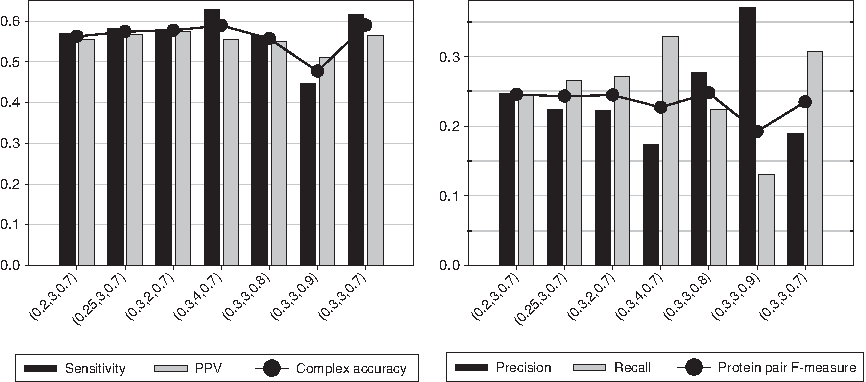
Performance of our algorithm NDComplex on the protein interaction network from the BioGRID database with respect to the complex accuracy measure and the protein pair agreement measure over different parameter settings (t,c,d), where t and c are the similarity threshold and the occurrence threshold, respectively, during the computation of neighborhood density, and d is the density threshold during the computation of predicted complexes in regions with low neighborhood density. The similarity threshold during the computation of predicted complexes in regions with high neighborhood density is fixed to s = 0.2. The last set of parameters (0.3,3,0.7) is the one we chose.

To illustrate the differences in predictions that can be obtained from different algorithms, we examine the predicted complex from each algorithm on the BioGRID network that has the highest similarity to the true complex that contains the MAP kinase cascade of the pheromone response pathway and the filamentation/invasion pathway (Gustin et al., 1998) from the MIPS database. Figure 7 shows that CLIQUE finds the complex that contains the MAP kinase cascade of the filamentation/invasion pathway, while the protein Fus3 in the true complex is not included. NDComplex expands the complex to include two extra proteins Bem1 and Hek2, in addition to all the proteins in the true complex. COACH and DECAFF return the largest complexes that contain a few extra proteins, while MCL and MCODE do not return a complex that has overlap to the true complex.

FIG. 7.

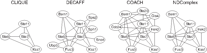
Predicted complex from each algorithm on the protein interaction network from the BioGRID database that has the highest similarity to the true complex that contains the MAP kinase cascade of the pheromone response pathway and the filamentation/invasion pathway from the MIPS database. No predicted complexes from MCL or MCODE have overlap to the true complex and are not shown.

One drawback of our algorithm is that it takes exponential time to identify all the maximal cliques, thus it is not likely that it will scale up to handle dense networks. One future direction is to investigate whether it is possible to develop polynomial time heuristics without a large decrease in prediction performance.

Footnotes

Acknowledgment

This work was supported by grants from the National Science Foundation (CCF-0830455, MCB-0951120).

Disclosure Statement

The authors declare that no competing financial interests exist.

References

Aloy

, Böttcher

, Ceulemans

et al. 2004. Structure-based assembly of protein complexes in yeast. Science, 303:2026–2029.

Altaf-Ul-Amin

, Shinbo

, Mihara

et al. 2006. Development and implementation of an algorithm for detection of protein complexes in large interaction networks. BMC Bioinformatics, 7:207.

Bader

G.D.

, Hogue

C.W.

2003. An automated method for finding molecular complexes in large protein interaction networks. BMC Bioinformatics, 4:2.

Brohée

, van Helden

2006. Evaluation of clustering algorithms for protein-protein interaction networks. BMC Bioinformatics, 7:488.

Cherry

J.M.

, Adler

, Ball

et al. 1998. SGD: Saccharomyces Genome Database. Nucleic Acids Res., 26:73–79.

Chua

H.N.

, Ning

, Sung

W.-K.

et al. 2008. Using indirect protein-protein interactions for protein complex prediction. J. Bioinformatics Comput. Biol., 6:435–466.

Enright

A.J.

, Van Dongen

, Ouzounis

C.A.

2002. An efficient algorithm for large-scale detection of protein families. Nucleic Acids Res., 30:1575–1584.

Friedel

C.C.

, Krumsiek

, Zimmer

2009. Bootstrapping the interactome: unsupervised identification of protein complexes in yeast. J. Comput. Biol., 16:971–987.

Gavin

A.-C.

, Bösche

, Krause

et al. 2002. Functional organization of the yeast proteome by systematic analysis of protein complexes. Nature, 415:141–147.

10.

Gustin

M.C.

, Albertyn

, Alexander

, Davenport

1998. MAP kinase pathways in the yeast Saccharomyces cerevisiae. Microbiol. Mol. Biol. Rev., 62:1264–1300.

11.

Hirsh

, Sharan

2007. Identification of conserved protein complexes based on a model of protein network evolution. Bioinformatics, 23:E170–176.

12.

, Gruhler

, Heilbut

et al. 2002. Systematic identification of protein complexes in Saccharomyces cerevisiae by mass spectrometry. Nature, 415:180–183.

13.

Jung

S.H.

, Hyun

, Jang

W.-H.

et al. 2010. Protein complex prediction based on simultaneous protein interaction network. Bioinformatics, 26:385–391.

14.

King

A.D.

, Pržulj

, Jurisica

2004. Protein complex prediction via cost-based clustering. Bioinformatics, 20:3013–3020.

15.

Krogan

N.J.

, Cagney

, Yu

et al. 2006. Global landscape of protein complexes in the yeast Saccharomyces cerevisiae. Nature, 440:637–643.

16.

Leung

H.C.M.

, Xiang

, Yiu

S.M.

, Chin

F.Y.L.

2009. Predicting protein complexes from PPI data: a core-attachment approach. J. Comput. Biol., 16:133–144.

17.

X.-L.

, Foo

C.-S.

, Ng

S.-K.

2007. Discovering protein complexes in dense reliable neighborhoods of protein interaction networks. Proc. 6th Ann. Int. Conf. Comput. Sys. Bioinformatics (CSB 2007), 157–168.

18.

Liu

, Wong

, Chua

H.N.

2009. Complex discovery from weighted PPI networks. Bioinformatics, 25:1891–1897.

19.

Mewes

H.W.

, Amid

, Arnold

et al. 2004. MIPS: analysis and annotation of proteins from whole genomes. Nucleic Acids Res., 32:D41–44.

20.

Moschopoulos

C.N.

, Pavlopoulos

G.A.

, Schneider

et al. 2009. GIBA: a clustering tool for detecting protein complexes. BMC Bioinformatics, 10,Suppl 6:S11.

21.

, Balem

, Faloutsos

et al. 2008. Protein complex identification by supervised graph local clustering. Bioinformatics, 24:I250–258.

22.

Sharan

, Ideker

, Kelley

et al. 2005. Identification of protein complexes by comparative analysis of yeast and bacterial protein interaction data. J. Comput. Biol., 12:835–846.

23.

Shi

, Lei

, Zhang

2011. Protein complex detection with semi-supervised learning in protein interaction networks. Proteome Sci., 9,Suppl 1:S5.

24.

Spirin

, Mirny

L.A.

2003. Protein complexes and functional modules in molecular networks. Proc. Natl. Acad. Sci. USA, 100:12123–12128.

25.

Stark

, Breitkreutz

B.-J.

, Reguly

et al. 2006. BioGRID: a general repository for interaction datasets. Nucleic Acids Res., 34:D535–539.

26.

, Chen

, Xu

2011. A binary matrix factorization algorithm for protein complex prediction. Proteome Sci., 9,Suppl 1:S18.

27.

, Li

, Kwoh

C.-K.

, Ng

S.-K.

2009. A core-attachment based method to detect protein complexes in PPI networks. BMC Bioinformatics, 10:169.

28.

Xenarios

, Rice

D.W.

, Salwinski

et al. 2000. DIP: the Database of Interacting Proteins. Nucleic Acids Res., 28:289–291.