Analyzing the basic mechanism of DNA double-strand breaks (DSB) formation during meiosis is important for understanding sexual reproduction and genetic diversity. The location and amount of meiotic DSBs can be examined by using a common molecular biological technique called Southern blotting, but only a subset of the total DSBs can be observed; only DSB fragments still carrying the region recognized by a Southern blot probe are detected. With the assumption that DSB formation follows a nonhomogeneous Poisson process, we propose two estimators of the total number of DSBs on a chromosome: (1) an estimator based on the Nelson-Aalen estimator, and (2) an estimator based on a record value process. Further, we compared their asymptotic accuracy.
1. Introduction
Meiosis is a specialized cell cycle essential for producing gametes in sexual reproduction (Petronczki et al., 2003). During meiosis, DNA double-strand breaks (DSBs) are programmed to be formed, and they induce homologous recombination. The homologous recombination mechanism facilitates recognition of homologous chromosomes and establishes physical connections between them (i.e., crossovers). The study on meiotic DSB formation and homologous recombination is important because it is not only central to the life cycle of sexually reproducing organisms but a driving force for producing genetic diversity.
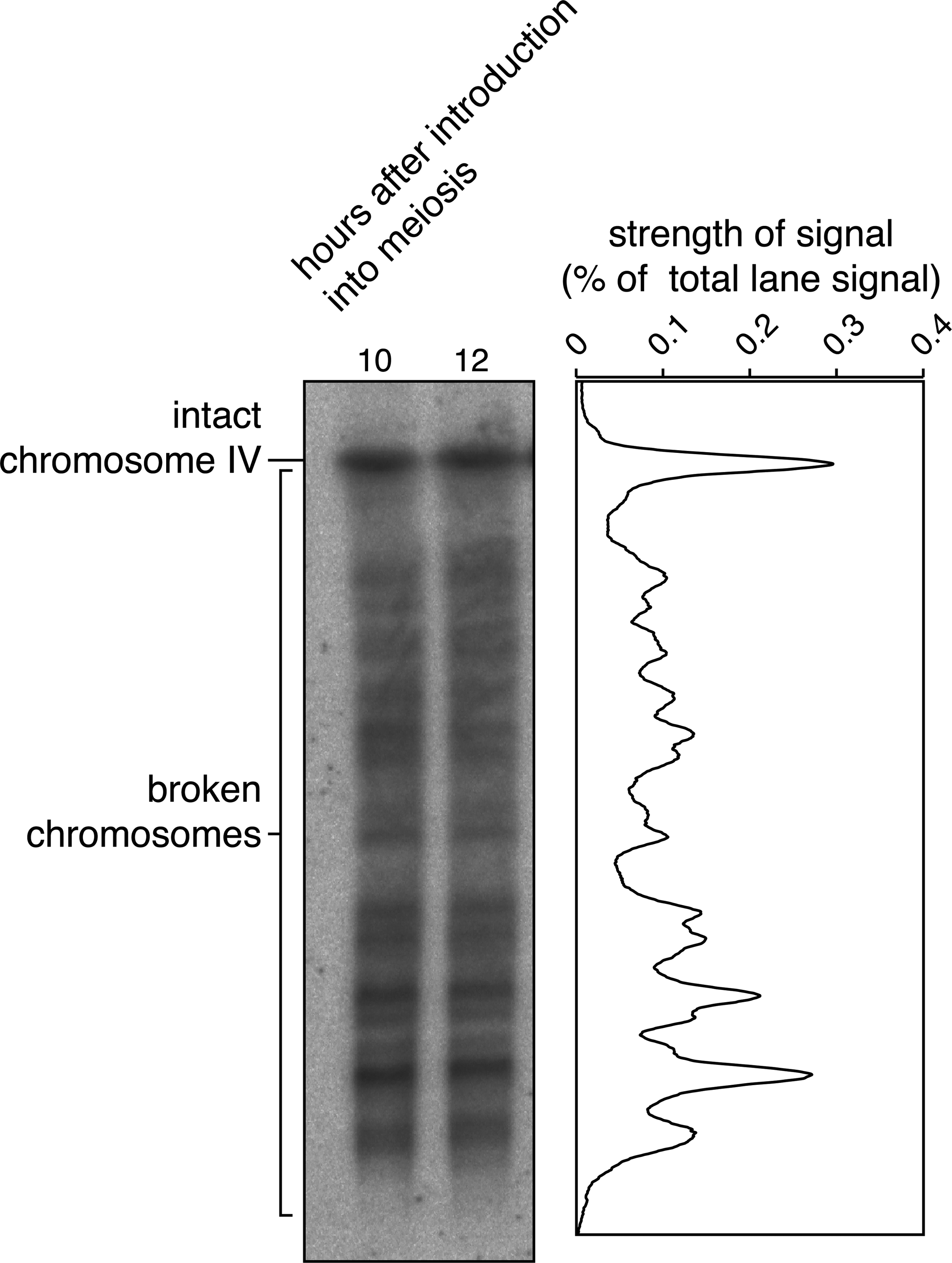
Meiotic DSB formation is controlled by many complex biological processes and the mechanism has been intensively studied using various methods (Keeney, 2001). Although meiotic DSB formation happens throughout the genome (consisting of multiple chromosomes with different length), the analysis of DSB formation, with respect to location and frequency, becomes much easier if one chromosome is examined at a time. A common molecular biological technique called Southern blotting enables detection of one unique location in the genome, making it possible to examine DSB formation per one given chromosome (Fig. 1) (Farmer et al., 2012, 2011). In short, the total genomic DNA prepared from cells introduced into meiosis is separated according to size by gel electrophoresis. The separated DNA molecules are transferred to a nylon membrane, on which DSB fragments carrying one end of a chromosome to be examined are labeled with a radioactive DNA probe. Thus, when a chromosome is intact (i.e., no DSBs are formed), only a single band appears at the location corresponding to the size of the whole chromosome. Once DSBs are formed, chromosomal DNA is broken and smaller molecular pieces appear accordingly, producing numerous bands below the position of the intact chromosome.
An example of double-strand break (DSB) detection by Southern blotting. Budding yeast diploid cells were introduced into meiosis, and cells were harvested at 10 and 12 hours after introduction into meiosis when amount of broken chromosomes are maximum. Genomic DNA was prepared from the samples and was separated by pulsed-field gel electrophoresis. The separated DNA samples were transferred to a nylon membrane, and chromosome IV was detected by Southern blotting using a probe that labels one end of chromosome IV (left). Lane profiles of 10 and 12 hours in each mutant background were normalized and averaged to obtain the profiles shown on the right (Farmer et al., 2011, 2012). A strain homozygous for the sae2 mutation was employed, in which DSBs are not repaired.
Although this method is suitable for determining the location of DSBs along chromosomes, the strength of the signal at a given location does not necessarily correlate with the actual number of DSBs formed there. This is because, when two or more DSBs are formed on a chromosome, only a DNA fragment carrying the chromosome end labeled by the probe is detected, while others are invisible. In other words, the total number of DSBs formed per chromosome is unknown using this approach.
In this work, we sought out to establish a method to estimate the total number of DSBs per chromosome using this kind of partial observation. In a large part of past linkage analysis, genetic recombination, which is the consequence of DSB formation, has been assumed to be a nonhomogeneous Poisson process (McPeek and Speed, 1995; Haldane, 1919). In the context of survival analysis with the partial observation, the nonparametric Nelson-Aalen estimator has been intensively used for estimating the cumulated hazard rate from censored data (Andersen et al., 1985); Andersen, 1993; Fleming and Harrington, 1991). Here, by simply assuming a nonhomogeneous Poisson process for DSB formation, we extend the idea of the Nelson-Aalen estimator to estimate the expected number of DSBs on a chromosome. In addition, based on record value processes (Ross, 1996; Shorrock, 1972), which are known to be related to nonhomogeneous Poisson processes, another type of estimator is proposed, and the accuracy of this estimator is compared with the accuracy of the former estimator.
2. Observing DSBS
Let N be the number of DSBs on a chromosome of the size c. We assume the chromosome is indexed by the position t from the left end (t = 0 is the left end and t = c is the right end). Let Tn be the nth break from the left end if there are any. Particularly, T1 represents the size of fragments sharing one end of the chromosome. All breaks but T1 are not observable in the experiments. Define the probability distribution of T1 as F(x) = P{T1 ≤ x}, which is assumed to be continuous and differentiable for simplicity. Since T1 is censored at c, the probability distribution of T1 is defective, and let p = P{T1 ≤ c} = F(c) be the probability that there is at least one break in the chromosome. Let h(x) be the hazard rate function of T1, which is defined as
\documentclass{aastex}\usepackage{amsbsy}\usepackage{amsfonts}\usepackage{amssymb}\usepackage{bm}\usepackage{mathrsfs}\usepackage{pifont}\usepackage{stmaryrd}\usepackage{textcomp}\usepackage{portland, xspace}\usepackage{amsmath, amsxtra}\pagestyle{empty}\DeclareMathSizes{10}{9}{7}{6}\begin{document}\begin{align*}h (x) dx = P \ {x \leq T_ {1} < x + dx \mid T_{1} \geq x} = \frac {f(x) dx} {1 - F(x)} , \tag {1}\end{align*}
\end{document}
where f (x) = dF(x)/dx is the density of the random variable T1. The probability distribution function can be recovered by the corresponding hazard rate function by using the formula:
\documentclass{aastex}\usepackage{amsbsy}\usepackage{amsfonts}\usepackage{amssymb}\usepackage{bm}\usepackage{mathrsfs}\usepackage{pifont}\usepackage{stmaryrd}\usepackage{textcomp}\usepackage{portland, xspace}\usepackage{amsmath, amsxtra}\pagestyle{empty}\DeclareMathSizes{10}{9}{7}{6}\begin{document}\begin{align*}F ( x ) = 1 - e^{- \int_{0}^{x}h ( s ) ds}. \tag{2}\end{align*}\end{document}
3. Nonhomogeneous Poisson Process N(t) and the First Break Point T1
Chromosomal context influences DSB formation, and there are specific regions called recombination hot spots in which DSBs are preferentially formed (Buhler et al., 2007). In the following, we assume DSBs follow a nonhomogeneous Poisson process. By doing so, we implicitly assume meiotic DSB formations have no strong interaction among them. During meiosis, some DSBs are repaired but some become crossovers between homologous chromosomes, and it is known that there is a phenomenon called crossover interference, reflecting a mechanism for discouraging two crossovers from forming in their neighborhood (Berchowitz and Copenhaver, 2010; McPeek and Speed, 1995). However, it is not known if there is a similar interference mechanism operating at the level of DSB formation.
Let N(t) be the number of breaks in the region (0,t]. The stochastic intensity of N(t) is defined by
\documentclass{aastex}\usepackage{amsbsy}\usepackage{amsfonts}\usepackage{amssymb}\usepackage{bm}\usepackage{mathrsfs}\usepackage{pifont}\usepackage{stmaryrd}\usepackage{textcomp}\usepackage{portland, xspace}\usepackage{amsmath, amsxtra}\pagestyle{empty}\DeclareMathSizes{10}{9}{7}{6}\begin{document}\begin{align*}\lambda ( t ) = \lim_ {\Delta t \to 0} \frac {E [ N ( t + \Delta t ) - N ( t ) \mid N ( s ) , 0 \leq s < t ]} {\Delta t} . \tag {3} \end{align*}\end{document}
In general point processes, λ(t) depends on the past (left) history {N(s), 0 ≤ s < t]} and becomes a stochastic process, but λ(t) is a deterministic function of t if and only if N(t) is a nonhomogeneous Poisson process (see Bacceili and Bremaud, 1994, for example).
The hazard rate function of the first event T1 is known to coincide with the intensity λ(t) of nonhomogeneous Poisson processes. Indeed, since there is only one event in an infinitesimally small dt, we have
\documentclass{aastex}\usepackage{amsbsy}\usepackage{amsfonts}\usepackage{amssymb}\usepackage{bm}\usepackage{mathrsfs}\usepackage{pifont}\usepackage{stmaryrd}\usepackage{textcomp}\usepackage{portland, xspace}\usepackage{amsmath, amsxtra}\pagestyle{empty}\DeclareMathSizes{10}{9}{7}{6}\begin{document}\begin{align*}h ( t ) dt = P \{t \leq T_{1} < t + dt \mid T_{1} \geq t \} & = P \{N ( t + dt ) - N ( t ) = 1 \mid N ( t ) = 0 \} \\ & = E [ N ( t + dt ) - N ( t ) \mid N ( t ) = 0 ] \\ & = \lambda ( t ) dt.\end{align*}\end{document}
By the inverse formula for hazard rate function Equation (2), we have the relationship:
\documentclass{aastex}\usepackage{amsbsy}\usepackage{amsfonts}\usepackage{amssymb}\usepackage{bm}\usepackage{mathrsfs}\usepackage{pifont}\usepackage{stmaryrd}\usepackage{textcomp}\usepackage{portland, xspace}\usepackage{amsmath, amsxtra}\pagestyle{empty}\DeclareMathSizes{10}{9}{7}{6}\begin{document}\begin{align*}E [ N ] = \int_{0}^{c} \lambda ( t ) dt = \int_{0}^{c} h ( t ) dt = - \log ( 1 - p ) . \tag{4}\end{align*}\end{document}
Alternatively, Equation (4) can be proven by the fact that N is a Poisson random variable and \documentclass{aastex}\usepackage{amsbsy}\usepackage{amsfonts}\usepackage{amssymb}\usepackage{bm}\usepackage{mathrsfs}\usepackage{pifont}\usepackage{stmaryrd}\usepackage{textcomp}\usepackage{portland, xspace}\usepackage{amsmath, amsxtra}\pagestyle{empty}\DeclareMathSizes{10}{9}{7}{6}\begin{document}$$1 - p = P \{N = 0 \} = \exp \{ - \int_{0}^{c} \lambda ( t ) dt \} $$\end{document}.
Furthermore, it is known that events of nonhomogeneous Poisson process can be constructed by the record value process (Ross, 1996; Shorrock, 1972). Prepare a sequence of independent and identically distributed samples \documentclass{aastex}\usepackage{amsbsy}\usepackage{amsfonts}\usepackage{amssymb}\usepackage{bm}\usepackage{mathrsfs}\usepackage{pifont}\usepackage{stmaryrd}\usepackage{textcomp}\usepackage{portland, xspace}\usepackage{amsmath, amsxtra}\pagestyle{empty}\DeclareMathSizes{10}{9}{7}{6}\begin{document}$$X_{1} , X_{2} , \ldots$$\end{document} that have the hazard rate function λ(t). Records Tn are recursively defined. Set T1 = X1 as the initial record. When a sample Xi exceeds the previous record Tn, its value is registered as the new record Tn+1. The nth record corresponds to the nth event epoch of nonhomogeneous Poisson process N(t) with the intensity λ(t). Indeed,
\documentclass{aastex}\usepackage{amsbsy}\usepackage{amsfonts}\usepackage{amssymb}\usepackage{bm}\usepackage{mathrsfs}\usepackage{pifont}\usepackage{stmaryrd}\usepackage{textcomp}\usepackage{portland, xspace}\usepackage{amsmath, amsxtra}\pagestyle{empty}\DeclareMathSizes{10}{9}{7}{6}\begin{document}\begin{align*} & E [ N ( t + dt ) - N ( t ) \mid N ( s ) , 0 \leq s < t ] = P \ \{{\rm a \ new \ record \ is \ in} \ [ t , t + dt ) \mid N ( s ) , 0 \leq s < t \} \\ & \quad= P \ \{ {\rm a \ new \ record \ is \ in} \ [ t , t + dt ) \} = P \{ t < X \leq t + dt \mid X > t \} = \lambda ( t ) dt , \end{align*}\end{document}
since the event of a new record greater than t is independent with the past history of records smaller than t. Thus, nonhomogenous Poisson processes can be stochastically reconstructed by the collection of independent and identically distributed samples of their own first event.
4. Three Estimators of E[N]
Because only the first break can be observed, we cannot use \documentclass{aastex}\usepackage{amsbsy}\usepackage{amsfonts}\usepackage{amssymb}\usepackage{bm}\usepackage{mathrsfs}\usepackage{pifont}\usepackage{stmaryrd}\usepackage{textcomp}\usepackage{portland, xspace}\usepackage{amsmath, amsxtra}\pagestyle{empty}\DeclareMathSizes{10}{9}{7}{6}\begin{document}$$\bar {N}$$\end{document}, the sample average of the number of breaks, to estimate E[N]. Instead, we propose three different estimators for E[N] and compare them.
Let \documentclass{aastex}\usepackage{amsbsy}\usepackage{amsfonts}\usepackage{amssymb}\usepackage{bm}\usepackage{mathrsfs}\usepackage{pifont}\usepackage{stmaryrd}\usepackage{textcomp}\usepackage{portland, xspace}\usepackage{amsmath, amsxtra}\pagestyle{empty}\DeclareMathSizes{10}{9}{7}{6}\begin{document}$$X_{1} , X_{2} , \ldots , X_{m}$$\end{document} be m identically distributed samples of the first breaks T1. Define \documentclass{aastex}\usepackage{amsbsy}\usepackage{amsfonts}\usepackage{amssymb}\usepackage{bm}\usepackage{mathrsfs}\usepackage{pifont}\usepackage{stmaryrd}\usepackage{textcomp}\usepackage{portland, xspace}\usepackage{amsmath, amsxtra}\pagestyle{empty}\DeclareMathSizes{10}{9}{7}{6}\begin{document}$$L ( t ) = \sum\nolimits_{i = 1}^{m}1_{\{X_{i} \leq t \}}$$\end{document}, which is the right continuous function representing the number of samples smaller than or equal to t, and define L0 by the number of unbroken samples. Based on Equation (4), we can construct an estimator of E[N] denoted by \documentclass{aastex}\usepackage{amsbsy}\usepackage{amsfonts}\usepackage{amssymb}\usepackage{bm}\usepackage{mathrsfs}\usepackage{pifont}\usepackage{stmaryrd}\usepackage{textcomp}\usepackage{portland, xspace}\usepackage{amsmath, amsxtra}\pagestyle{empty}\DeclareMathSizes{10}{9}{7}{6}\begin{document}$$\hat N_{\alpha}$$\end{document} as
\documentclass{aastex}\usepackage{amsbsy}\usepackage{amsfonts}\usepackage{amssymb}\usepackage{bm}\usepackage{mathrsfs}\usepackage{pifont}\usepackage{stmaryrd}\usepackage{textcomp}\usepackage{portland, xspace}\usepackage{amsmath, amsxtra}\pagestyle{empty}\DeclareMathSizes{10}{9}{7}{6}\begin{document}\begin{align*}\hat {N} _ {\alpha} = - \log \left( \frac {L_ {0}} {m} \right) . \tag {5} \end{align*}\end{document}
Since P{L0 = 0} > 0, all moments of this estimator is infinite, so we need to be cautious with using this estimator (Peña and Rohatgi, 1993).
Alternatively, since Equation (4) can also be interpreted as the cumulated hazard rate function, we can use the Nelson-Aalen estimator (see Fleming and Harrington, 1991, for example);
\documentclass{aastex}\usepackage{amsbsy}\usepackage{amsfonts}\usepackage{amssymb}\usepackage{bm}\usepackage{mathrsfs}\usepackage{pifont}\usepackage{stmaryrd}\usepackage{textcomp}\usepackage{portland, xspace}\usepackage{amsmath, amsxtra}\pagestyle{empty}\DeclareMathSizes{10}{9}{7}{6}\begin{document}\begin{align*}\hat N_ {\beta} = \int_ {0} ^ {c} \frac {dL ( s )} {Y ( s )} = \frac {1} {m} + \frac {1} {m - 1} + \cdots + \frac {1} {L_ {0} + 1} = \sum_ {i = L_ {0} + 1} ^ {m} \frac {1} {i} \tag {6} \end{align*}\end{document}
where \documentclass{aastex}\usepackage{amsbsy}\usepackage{amsfonts}\usepackage{amssymb}\usepackage{bm}\usepackage{mathrsfs}\usepackage{pifont}\usepackage{stmaryrd}\usepackage{textcomp}\usepackage{portland, xspace}\usepackage{amsmath, amsxtra}\pagestyle{empty}\DeclareMathSizes{10}{9}{7}{6}\begin{document}$$Y ( t ) = \sum\nolimits_{i = 1}^{m}1_{\{X_{i} > t \}}$$\end{document} is called the number of samples in risk in the position t. In general, Nelson-Aalen estimator \documentclass{aastex}\usepackage{amsbsy}\usepackage{amsfonts}\usepackage{amssymb}\usepackage{bm}\usepackage{mathrsfs}\usepackage{pifont}\usepackage{stmaryrd}\usepackage{textcomp}\usepackage{portland, xspace}\usepackage{amsmath, amsxtra}\pagestyle{empty}\DeclareMathSizes{10}{9}{7}{6}\begin{document}$$\hat N_{\beta}$$\end{document} is used to estimate the cumulated hazard rate function from censored data in survival analysis and then used for estimating the survival probability P{T1 > t}. As seen in the following, \documentclass{aastex}\usepackage{amsbsy}\usepackage{amsfonts}\usepackage{amssymb}\usepackage{bm}\usepackage{mathrsfs}\usepackage{pifont}\usepackage{stmaryrd}\usepackage{textcomp}\usepackage{portland, xspace}\usepackage{amsmath, amsxtra}\pagestyle{empty}\DeclareMathSizes{10}{9}{7}{6}\begin{document}$$\hat N_{\alpha}$$\end{document} and \documentclass{aastex}\usepackage{amsbsy}\usepackage{amsfonts}\usepackage{amssymb}\usepackage{bm}\usepackage{mathrsfs}\usepackage{pifont}\usepackage{stmaryrd}\usepackage{textcomp}\usepackage{portland, xspace}\usepackage{amsmath, amsxtra}\pagestyle{empty}\DeclareMathSizes{10}{9}{7}{6}\begin{document}$$\hat N_{\beta}$$\end{document} are asymptotically equivalent. In a sense, the way we used the estimator \documentclass{aastex}\usepackage{amsbsy}\usepackage{amsfonts}\usepackage{amssymb}\usepackage{bm}\usepackage{mathrsfs}\usepackage{pifont}\usepackage{stmaryrd}\usepackage{textcomp}\usepackage{portland, xspace}\usepackage{amsmath, amsxtra}\pagestyle{empty}\DeclareMathSizes{10}{9}{7}{6}\begin{document}$$\hat N_{\alpha}$$\end{document} is the reverse of survival analysis. We summarize the properties for both estimators including known facts about Nelson-Aalen estimator (Fleming and Harrington, 1991).
Theorem 1
The estimator\documentclass{aastex}\usepackage{amsbsy}\usepackage{amsfonts}\usepackage{amssymb}\usepackage{bm}\usepackage{mathrsfs}\usepackage{pifont}\usepackage{stmaryrd}\usepackage{textcomp}\usepackage{portland, xspace}\usepackage{amsmath, amsxtra}\pagestyle{empty}\DeclareMathSizes{10}{9}{7}{6}\begin{document}$$\hat N_{\alpha}$$\end{document}and\documentclass{aastex}\usepackage{amsbsy}\usepackage{amsfonts}\usepackage{amssymb}\usepackage{bm}\usepackage{mathrsfs}\usepackage{pifont}\usepackage{stmaryrd}\usepackage{textcomp}\usepackage{portland, xspace}\usepackage{amsmath, amsxtra}\pagestyle{empty}\DeclareMathSizes{10}{9}{7}{6}\begin{document}$$\hat N_{\beta}$$\end{document}for N have the following relationships:
as m → ∞. In addition,\documentclass{aastex}\usepackage{amsbsy}\usepackage{amsfonts}\usepackage{amssymb}\usepackage{bm}\usepackage{mathrsfs}\usepackage{pifont}\usepackage{stmaryrd}\usepackage{textcomp}\usepackage{portland, xspace}\usepackage{amsmath, amsxtra}\pagestyle{empty}\DeclareMathSizes{10}{9}{7}{6}\begin{document}\begin{align*}\lim_{m \to \infty} \hat N_{\beta} = E [ N ] \ a.s. \tag{8}\end{align*}\end{document}
2. Both estimators have the same asymptotic:\documentclass{aastex}\usepackage{amsbsy}\usepackage{amsfonts}\usepackage{amssymb}\usepackage{bm}\usepackage{mathrsfs}\usepackage{pifont}\usepackage{stmaryrd}\usepackage{textcomp}\usepackage{portland, xspace}\usepackage{amsmath, amsxtra}\pagestyle{empty}\DeclareMathSizes{10}{9}{7}{6}\begin{document}\begin{align*}m^{1 / 2} (\hat N_{\alpha} - E [N]) \mathop \rightarrow^{d} \sigma N ( 0 , 1 ) , \tag{9}\end{align*}\end{document}\documentclass{aastex}\usepackage{amsbsy}\usepackage{amsfonts}\usepackage{amssymb}\usepackage{bm}\usepackage{mathrsfs}\usepackage{pifont}\usepackage{stmaryrd}\usepackage{textcomp}\usepackage{portland, xspace}\usepackage{amsmath, amsxtra}\pagestyle{empty}\DeclareMathSizes{10}{9}{7}{6}\begin{document}\begin{align*}m^{1 / 2} ( \hat N_{\beta} - E [ N ] )\mathop \rightarrow^{d} \sigma N ( 0 , 1 ) , \tag{10}\end{align*}\end{document}
as m → ∞, where σ = {p/(1−p)}1/2. Here, N(0, 1) is the standard normal distribution and\documentclass{aastex}\usepackage{amsbsy}\usepackage{amsfonts}\usepackage{amssymb}\usepackage{bm}\usepackage{mathrsfs}\usepackage{pifont}\usepackage{stmaryrd}\usepackage{textcomp}\usepackage{portland, xspace}\usepackage{amsmath, amsxtra}\pagestyle{empty}\DeclareMathSizes{10}{9}{7}{6}\begin{document}$$\mathop \rightarrow^{d}$$\end{document}means convergence in distribution.
Proof
For the first part, because of the law of large numbers, L0/m → 1−p and log(L0/m) → log(1−p) =−E[N] a.s. as m → ∞. Also, it is well known that the difference between the harmonic series and logarithm converges to Euler-Mascheroni constant γ;
\documentclass{aastex}\usepackage{amsbsy}\usepackage{amsfonts}\usepackage{amssymb}\usepackage{bm}\usepackage{mathrsfs}\usepackage{pifont}\usepackage{stmaryrd}\usepackage{textcomp}\usepackage{portland, xspace}\usepackage{amsmath, amsxtra}\pagestyle{empty}\DeclareMathSizes{10}{9}{7}{6}\begin{document}\begin{align*}\lim_ {m \to \infty} \left( \sum_ {i = 1} ^ {m } \frac {1} {i} - \log m \right) = \lim_ {m \to \infty} \int_ {1} ^ {m} \left( \frac {1} {\lfloor x \rfloor} - \frac {1} {x} \right) dx = \gamma. \tag {11} \end{align*}\end{document}
as m → ∞, and also it is clear that \documentclass{aastex}\usepackage{amsbsy}\usepackage{amsfonts}\usepackage{amssymb}\usepackage{bm}\usepackage{mathrsfs}\usepackage{pifont}\usepackage{stmaryrd}\usepackage{textcomp}\usepackage{portland, xspace}\usepackage{amsmath, amsxtra}\pagestyle{empty}\DeclareMathSizes{10}{9}{7}{6}\begin{document}$$\hat N_{\alpha}$$\end{document} is always larger than \documentclass{aastex}\usepackage{amsbsy}\usepackage{amsfonts}\usepackage{amssymb}\usepackage{bm}\usepackage{mathrsfs}\usepackage{pifont}\usepackage{stmaryrd}\usepackage{textcomp}\usepackage{portland, xspace}\usepackage{amsmath, amsxtra}\pagestyle{empty}\DeclareMathSizes{10}{9}{7}{6}\begin{document}$$\hat N_{\beta}$$\end{document}. Nelson-Aalen estimator is known to be asymptotically unbiased. Indeed,
\documentclass{aastex}\usepackage{amsbsy}\usepackage{amsfonts}\usepackage{amssymb}\usepackage{bm}\usepackage{mathrsfs}\usepackage{pifont}\usepackage{stmaryrd}\usepackage{textcomp}\usepackage{portland, xspace}\usepackage{amsmath, amsxtra}\pagestyle{empty}\DeclareMathSizes{10}{9}{7}{6}\begin{document}\begin{align*}M (t) = \int_{0}^{t} \frac {dL (s)} {Y (s)} -
\int_{0}^{t} 1_ {\{ Y(s) > 0\}} h (s) ds \tag {13}
\end{align*}\end{document}
is zero-mean martingale (Fleming and Harrington, 1991), and
\documentclass{aastex}\usepackage{amsbsy}\usepackage{amsfonts}\usepackage{amssymb}\usepackage{bm}\usepackage{mathrsfs}\usepackage{pifont}\usepackage{stmaryrd}\usepackage{textcomp}\usepackage{portland, xspace}\usepackage{amsmath, amsxtra}\pagestyle{empty}\DeclareMathSizes{10}{9}{7}{6}\begin{document}\begin{align*}0 \leq E [ N ] - E [ \hat N_{\beta} ] & = E \left[ \int_{0}^{c}1_{\{Y ( s ) = 0 \}}h ( s ) ds \right] = \int_{0}^{c}P{\{Y ( s ) = 0 \}}h ( s ) ds \\ & = \int_{0}^{c} ( F ( s ) ) ^{m}h ( s ) ds \leq p^{m} \int_{0}^{c} \lambda ( s ) ds \to 0 , \end{align*}\end{document}
as m → ∞. For the second part, it is also known from martingale central limit theory (Fleming and Harrington, 1991) that
\documentclass{aastex}\usepackage{amsbsy}\usepackage{amsfonts}\usepackage{amssymb}\usepackage{bm}\usepackage{mathrsfs}\usepackage{pifont}\usepackage{stmaryrd}\usepackage{textcomp}\usepackage{portland, xspace}\usepackage{amsmath, amsxtra}\pagestyle{empty}\DeclareMathSizes{10}{9}{7}{6}\begin{document}\begin{align*}m^{1 / 2} ( \hat N_{\beta} - E [ N ] ) \mathop \rightarrow^{d} \sigma N ( 0 , 1 ) , \tag{14}\end{align*}\end{document}
where
\documentclass{aastex}\usepackage{amsbsy}\usepackage{amsfonts}\usepackage{amssymb}\usepackage{bm}\usepackage{mathrsfs}\usepackage{pifont}\usepackage{stmaryrd}\usepackage{textcomp}\usepackage{portland, xspace}\usepackage{amsmath, amsxtra}\pagestyle{empty}\DeclareMathSizes{10}{9}{7}{6}\begin{document}\begin{align*}\sigma^ {2} = \int_ {0} ^ {c} \frac {h ( s ) ds} {1 - F ( s )} . \tag {15} \end{align*}\end{document}
Since h(s) = f (s)/(1−F(s)), it is easy to show σ2 = p/(1−p). ■
Since \documentclass{aastex}\usepackage{amsbsy}\usepackage{amsfonts}\usepackage{amssymb}\usepackage{bm}\usepackage{mathrsfs}\usepackage{pifont}\usepackage{stmaryrd}\usepackage{textcomp}\usepackage{portland, xspace}\usepackage{amsmath, amsxtra}\pagestyle{empty}\DeclareMathSizes{10}{9}{7}{6}\begin{document}$$\hat N_{\alpha}$$\end{document} (and its asymptotically equivalent estimator \documentclass{aastex}\usepackage{amsbsy}\usepackage{amsfonts}\usepackage{amssymb}\usepackage{bm}\usepackage{mathrsfs}\usepackage{pifont}\usepackage{stmaryrd}\usepackage{textcomp}\usepackage{portland, xspace}\usepackage{amsmath, amsxtra}\pagestyle{empty}\DeclareMathSizes{10}{9}{7}{6}\begin{document}$$\hat N_{\beta}$$\end{document} as well) is based on the ratio of unbroken samples and fails to use full information of observed first break position, there may be some room for improvement. Thus, we came up with another estimator \documentclass{aastex}\usepackage{amsbsy}\usepackage{amsfonts}\usepackage{amssymb}\usepackage{bm}\usepackage{mathrsfs}\usepackage{pifont}\usepackage{stmaryrd}\usepackage{textcomp}\usepackage{portland, xspace}\usepackage{amsmath, amsxtra}\pagestyle{empty}\DeclareMathSizes{10}{9}{7}{6}\begin{document}$$\hat N_{\gamma}$$\end{document}, which is based on the renewal record value process employing first break samples as i.i.d. sequence. As seen in Section 3, the record value process of the first breaks Xi recovers a nonhomogeneous Poisson stream. Our data is censored, and each time we find a nonbreak sample, which happened with probability 1 – p, the Poisson event stream is terminated and restarted by selecting the first record. Repeat this renewal record value process S times, using m samples of Xi. From l th round of the record value process, we can construct Nl, the number of new records smaller than c. When the first sample is nonbreak, we set Nl = 0. Let Kl be the number of samples used in the l th round, including the non break sample. The estimator \documentclass{aastex}\usepackage{amsbsy}\usepackage{amsfonts}\usepackage{amssymb}\usepackage{bm}\usepackage{mathrsfs}\usepackage{pifont}\usepackage{stmaryrd}\usepackage{textcomp}\usepackage{portland, xspace}\usepackage{amsmath, amsxtra}\pagestyle{empty}\DeclareMathSizes{10}{9}{7}{6}\begin{document}$$\hat N_{\gamma}$$\end{document} is then defined by sample average of the i.i.d. sequence of Nl:
\documentclass{aastex}\usepackage{amsbsy}\usepackage{amsfonts}\usepackage{amssymb}\usepackage{bm}\usepackage{mathrsfs}\usepackage{pifont}\usepackage{stmaryrd}\usepackage{textcomp}\usepackage{portland, xspace}\usepackage{amsmath, amsxtra}\pagestyle{empty}\DeclareMathSizes{10}{9}{7}{6}\begin{document}\begin{align*}\hat N_ {\gamma} = \frac {1} {S} \sum_ {l = 1} ^ {S} N_ {l} . \tag {16} \end{align*}\end{document}
There is a positive correlation between Nl and Kl.
Because the samples Xi are i.i.d, the probability that the i th sample is the record value among i samples is always 1/i. This is still true even if we condition that the Poisson steam is terminated at Kl = k. Thus,
\documentclass{aastex}\usepackage{amsbsy}\usepackage{amsfonts}\usepackage{amssymb}\usepackage{bm}\usepackage{mathrsfs}\usepackage{pifont}\usepackage{stmaryrd}\usepackage{textcomp}\usepackage{portland, xspace}\usepackage{amsmath, amsxtra}\pagestyle{empty}\DeclareMathSizes{10}{9}{7}{6}\begin{document}\begin{align*}E [ N_ {l} \mid K_{l} = k ] = E \left[ \sum_{i =
1}^{k - 1} 1_{\{{\rm sample} \ i \ {\rm is} \ {\rm a} \ {\rm
record}\}} \mid K_ {l} = k \right] = \sum_ {i = 1}^ {k - 1} \frac
{1} {i} , \tag {18} \end{align*}\end{document}
where the summation is regarded as 0 when k = 1. Let \documentclass{aastex}\usepackage{amsbsy}\usepackage{amsfonts}\usepackage{amssymb}\usepackage{bm}\usepackage{mathrsfs}\usepackage{pifont}\usepackage{stmaryrd}\usepackage{textcomp}\usepackage{portland, xspace}\usepackage{amsmath, amsxtra}\pagestyle{empty}\DeclareMathSizes{10}{9}{7}{6}\begin{document}$$H_{k} = \sum_{i = 1}^{k}1 / i$$\end{document} be the kth harmonic number. Since Kl is a geometric random variable with the parameter 1−p, we have
\documentclass{aastex}\usepackage{amsbsy}\usepackage{amsfonts}\usepackage{amssymb}\usepackage{bm}\usepackage{mathrsfs}\usepackage{pifont}\usepackage{stmaryrd}\usepackage{textcomp}\usepackage{portland, xspace}\usepackage{amsmath, amsxtra}\pagestyle{empty}\DeclareMathSizes{10}{9}{7}{6}\begin{document}\begin{align*}E [ N_ {l} K_ {l} ] = E [ K_ {l} E [ N_ {l} \mid K_ {l} ] ] = E \left[ K_ {l} \sum_ {i = 1} ^ {K_ {l} - 1} \frac {1} {i} \right] = \sum_ {k = 1} ^ {\infty} k H_ {k - 1} p^ {k - 1} ( 1 - p )\end{align*}\end{document}
Using the fact \documentclass{aastex}\usepackage{amsbsy}\usepackage{amsfonts}\usepackage{amssymb}\usepackage{bm}\usepackage{mathrsfs}\usepackage{pifont}\usepackage{stmaryrd}\usepackage{textcomp}\usepackage{portland, xspace}\usepackage{amsmath, amsxtra}\pagestyle{empty}\DeclareMathSizes{10}{9}{7}{6}\begin{document}$$\sum\nolimits_{k = 1}^{\infty}H_{k}z^{k} = - \log ( 1 - z ) / ( 1 - z )$$\end{document}, we have
\documentclass{aastex}\usepackage{amsbsy}\usepackage{amsfonts}\usepackage{amssymb}\usepackage{bm}\usepackage{mathrsfs}\usepackage{pifont}\usepackage{stmaryrd}\usepackage{textcomp}\usepackage{portland, xspace}\usepackage{amsmath, amsxtra}\pagestyle{empty}\DeclareMathSizes{10}{9}{7}{6}\begin{document}\begin{align*}E [N_ {l} K_ {l}] = \frac {p - \log ( 1 - p )} {1
- p} , \tag {19} \end{align*}\end{document}
and the result follows from E[Nl] = −log(1−p) and E[Kl] = 1/(1−p). ■
Thus, Nl and S are negatively correlated, which generates larger fluctuation in \documentclass{aastex}\usepackage{amsbsy}\usepackage{amsfonts}\usepackage{amssymb}\usepackage{bm}\usepackage{mathrsfs}\usepackage{pifont}\usepackage{stmaryrd}\usepackage{textcomp}\usepackage{portland, xspace}\usepackage{amsmath, amsxtra}\pagestyle{empty}\DeclareMathSizes{10}{9}{7}{6}\begin{document}$$\hat N_{\gamma}$$\end{document} especially for a large p. To analyze the asymptotic of \documentclass{aastex}\usepackage{amsbsy}\usepackage{amsfonts}\usepackage{amssymb}\usepackage{bm}\usepackage{mathrsfs}\usepackage{pifont}\usepackage{stmaryrd}\usepackage{textcomp}\usepackage{portland, xspace}\usepackage{amsmath, amsxtra}\pagestyle{empty}\DeclareMathSizes{10}{9}{7}{6}\begin{document}$$\hat N_{\gamma}$$\end{document}, we need the following Anscombe's theorem.
Lemma 2
(see Rényi, 1957). Let Zi be a sequence of i.i.d random variable with E[Zi] = 0 and V ar[Zi] = 1, and U(t) be a positive integer random variable for t > 0, which may depend on Zi. If U(t)/t →μ in probability as t → ∞ for a positive deterministic constant μ, we have\documentclass{aastex}\usepackage{amsbsy}\usepackage{amsfonts}\usepackage{amssymb}\usepackage{bm}\usepackage{mathrsfs}\usepackage{pifont}\usepackage{stmaryrd}\usepackage{textcomp}\usepackage{portland, xspace}\usepackage{amsmath, amsxtra}\pagestyle{empty}\DeclareMathSizes{10}{9}{7}{6}\begin{document}\begin{align*}U ( t ) ^{- 1 / 2} \sum_{i = 1}^{U ( t )}Z_{i} \mathop\rightarrow^{d} N ( 0 , 1 ) , \tag{20}\end{align*}\end{document}
as t → ∞.
Theorem 2
The estimator\documentclass{aastex}\usepackage{amsbsy}\usepackage{amsfonts}\usepackage{amssymb}\usepackage{bm}\usepackage{mathrsfs}\usepackage{pifont}\usepackage{stmaryrd}\usepackage{textcomp}\usepackage{portland, xspace}\usepackage{amsmath, amsxtra}\pagestyle{empty}\DeclareMathSizes{10}{9}{7}{6}\begin{document}$$\hat N_{\gamma}$$\end{document}is consistent and has the asymptotic:\documentclass{aastex}\usepackage{amsbsy}\usepackage{amsfonts}\usepackage{amssymb}\usepackage{bm}\usepackage{mathrsfs}\usepackage{pifont}\usepackage{stmaryrd}\usepackage{textcomp}\usepackage{portland, xspace}\usepackage{amsmath, amsxtra}\pagestyle{empty}\DeclareMathSizes{10}{9}{7}{6}\begin{document}\begin{align*}m^{1 / 2} ( \hat N_{\gamma} - E [ N ] ) \mathop \rightarrow^{d} \sigma_{\gamma} N ( 0 , 1 ) , \tag{21}\end{align*}\end{document}
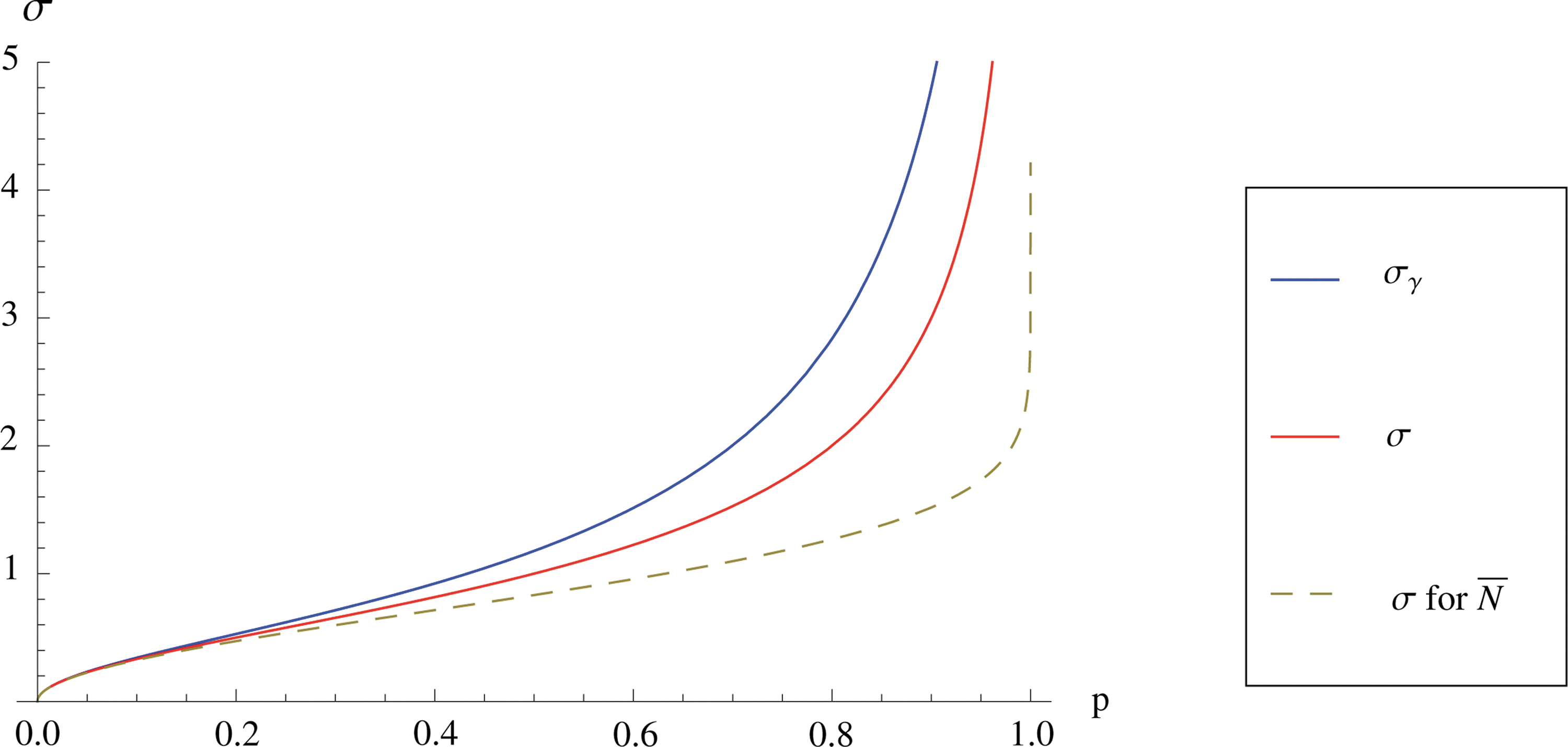
as m → ∞, where σγ = {−log(1−p)/(1−p)}1/2 > σ = {p/(1−p)}1/2for 0 < p < 1.
Proof
By renewal theorem, S/m → 1/E[K] a.s., as m → ∞. Thus, the consistency is immediate by law of large numbers. Further, since almost sure convergence implies convergence in probability, we can use Lemma 2 to have
\documentclass{aastex}\usepackage{amsbsy}\usepackage{amsfonts}\usepackage{amssymb}\usepackage{bm}\usepackage{mathrsfs}\usepackage{pifont}\usepackage{stmaryrd}\usepackage{textcomp}\usepackage{portland, xspace}\usepackage{amsmath, amsxtra}\pagestyle{empty}\DeclareMathSizes{10}{9}{7}{6}\begin{document}\begin{align*}S^{- 1 / 2} \sum_{l = 1}^{S} \frac {N_ {l} - E
[N]} {\{Var [N] \}^{1/2}} \mathop \rightarrow^{d} N (0 , 1) , \tag
{22} \end{align*}\end{document}
as m → ∞ . The result follows by noticing that N is a Poisson random variable and V ar[N] = E[N] = −log(1−p) and E[K] = 1/(1−p). ■
Figure 2 shows the comparison of asymptotic efficiency of estimators from Theorem 1 and 2. The sample average \documentclass{aastex}\usepackage{amsbsy}\usepackage{amsfonts}\usepackage{amssymb}\usepackage{bm}\usepackage{mathrsfs}\usepackage{pifont}\usepackage{stmaryrd}\usepackage{textcomp}\usepackage{portland, xspace}\usepackage{amsmath, amsxtra}\pagestyle{empty}\DeclareMathSizes{10}{9}{7}{6}\begin{document}$$\bar N$$\end{document}, which is not feasible for our experiments, is also displayed for the reference. Here, we can see a clear advantage of the estimator \documentclass{aastex}\usepackage{amsbsy}\usepackage{amsfonts}\usepackage{amssymb}\usepackage{bm}\usepackage{mathrsfs}\usepackage{pifont}\usepackage{stmaryrd}\usepackage{textcomp}\usepackage{portland, xspace}\usepackage{amsmath, amsxtra}\pagestyle{empty}\DeclareMathSizes{10}{9}{7}{6}\begin{document}$$\hat N_{\alpha}$$\end{document} and \documentclass{aastex}\usepackage{amsbsy}\usepackage{amsfonts}\usepackage{amssymb}\usepackage{bm}\usepackage{mathrsfs}\usepackage{pifont}\usepackage{stmaryrd}\usepackage{textcomp}\usepackage{portland, xspace}\usepackage{amsmath, amsxtra}\pagestyle{empty}\DeclareMathSizes{10}{9}{7}{6}\begin{document}$$\hat N_{\beta}$$\end{document}, especially for large p.
Comparison of asymptotic efficiency of estimators.
Footnotes
Disclosure Statement
No competing financial interests exist.
References
1.
AndersenP.1993. Statistical models based on counting processes. Springer Verlag: Heidelberg, Germany.
2.
AndersenP.K., BorganØ., HjortN.L., ArjasE., SteneJ., AalenO.1985. Counting process models for life history data: A review [with discussion and reply]Scandinavian Journal of Statistics, 12:97–158.
3.
BacceiliF., BremaudP.1994. Elements of Qeueing Theory. Springer-Verlag: Heidelberg, Germany.
4.
BerchowitzL., CopenhaverG.2010. Genetic interference: don't stand so close to me. Current Genomics, 11:91.
5.
BuhlerC., BordeV., LichtenM.2007. Mapping meiotic single-strand DNA reveals a new landscape of DNA double-strand breaks in saccharomyces cerevisiae. PLoS Biol., 5:e324.
6.
FarmerS., HongE.-J.E., LeungW.-K., ArgunhanB., TerentyevY., HumphryesN., ToyoizumiH., TsubouchiH.2012. Budding yeast pch2, a widely conserved meiotic protein, is involved in the initiation of meiotic recombination. PLoS ONE, 7:e39724.
7.
FarmerS., LeungW.-K., TsubouchiH.2011. Characterization of meiotic recombination initiation sites using pulsed-field gel electrophoresis. Methods in Molecular Biology, 745:33–45.
HaldaneJ.1919. The combination of linkage values and the calculation of distances between the loci of linked factors. J. Genet., 8:309.
10.
KeeneyS.2001. Mechanism and control of meiotic recombination initiation, 52:1–53. Academic Press: Waltham, MA.
11.
McPeekM.S., SpeedT.P.1995. Modeling interference in genetic recombination. Genetics, 139:1031–1044.
12.
PeñaE.A., RohatgiV.K.1993. Small sample and efficiency results for the Nelson-Aalen estimator. Journal of Statistical Planning and Inference, 37:193–202.
13.
PetronczkiM., SiomosM.F., NasmythK.2003. Un ménage àquatre: The molecular biology of chromosome segregation in meiosis. Cell, 112:423–440.
14.
RényiA.1957. On the asymptotic distribution of the sum of a random number of independent random variables. Acta Mathematica Hungarica, 8:193–199.
15.
RossS.M.1996. Stochastic Processes. John Wiley and Sons: Hoboken, NJ.
16.
ShorrockR.W.1972. On record values and record times. Journal of Applied Probability, 9:316–326.