Direct Updating of an RNA Base-Pairing Probability Matrix with Marginal Probability Constraints

1. Introduction

Non-coding RNAs (e.g., miRNA, snoRNA, piRNA, and lincRNA) play many important roles in life (Gardner et al., 2011), some of which are related to disease (Esteller, 2011). The secondary and tertiary structures of RNA sequences are a key to understanding their functions, and much research has been conducted in this field (Leontis and Westhof, 2012).

The base-pairing probability matrix (BPPM) of an RNA sequence, which stores all the probabilities for possible base pairs in an RNA sequence (see Section 2 for the detailed definition), has played an essential role in a number of algorithms in RNA informatics, including RNA (common) secondary structure predictions (Seemann et al., 2008,) Lu et al., 2009; Hamada et al., 2009b, 2011c; Sato et al., 2011, multiple alignment of RNA sequences (Hofacker et al., 2004; Katoh and Toh, 2008; Hamada et al., 2009a; Sahraeian and Yoon, 2011), RNA–RNA interaction predictions (Kato et al., 2010; Seemann et al., 2011), RNA motif search (Hamada et al., 2006), and miRNA gene finding (Terai et al., 2007) (Wei et al., 2011). Estimating accurate base-pairing probabilities, therefore, has the potential to improve those algorithms without modifying them.

On the other hand, the recent advent of experimental techniques to probe RNA structure by high-throughput sequencing—SHAPE (Low and Weeks, 2010); PARS (Kertesz et al., 2010); FragSeq (Underwood et al., 2010)—has enabled genome-wide measurements of RNA structure, leading to the world of the “RNA structurome” (Wan et al., 2011). Those experimental techniques (SHAPE, PARS, and FragSeq) stochastically estimate the flexibility of an RNA strand, which can be considered as a kind of loop probability for every nucleotide in an RNA sequence. Remarkably, secondary structures of long RNA sequences—HIV-1 (Watts et al., 2009), HCV (hepatitis C virus) (Pang et al., 2011), and lincRNA (the steroid receptor RNA activator [SRA]) (Novikova et al., 2012)—were recently determined by combining those experimental techniques with computational approaches. It is therefore important to incorporate this experimental information into RNA informatics, especially structural analysis for RNAs. Washietl et al. (2012) have proposed a method to modify the Turner energy parameters to be consistent with the experimental (SHAPE) data. Deigan et al. (2009) incorporated experimental information (given by SHAPE) into energy calculations of RNA secondary structure. (See Low and Weeks [2010] for recent reviews.) Quarrier et al. (2010) proposed a method to generate “decoy” RNA structures by stochastic sampling and evaluating whether the structure fits the constraints. However, there are many models for RNA secondary structures, such as Turner's energy model (McCaskill, 1990; Hofacker et al., 1994; Mathews et al., 1999) and the (machine learning) stochastic model (Do et al., 2006; Andronescu et al., 2007, 2010), and we must implement the algorithms separately for each model.

Against this background, we propose a novel lightweight and simple algorithm for updating the base-pairing probability matrix according to marginal probability constraints after formulating the problem mathematically. We found that the problem has a similar structure to estimating an input–output (IO) table in macroeconomics, which is called the matrix balancing problem (Censor and Zenios, 1997; Morioka and Tsuda, 2011). Therefore, our algorithms are based on the RAS algorithms used in macroeconomics. The algorithm is not only simple and fast but also easily implemented and widely applicable to models of RNA secondary structures that produce a base-pairing probability matrix. Most tools for predicting RNA secondary structures have an option to produce a base-paring probability matrix. ¹

This article is organized as follows. In Section 2, we mathematically formulate the targeted problem, which is followed by algorithms to solve the problem in Section 3, including the proof of validity of the algorithms. Preliminary computational experiments for confirming the effectiveness of the algorithms are discussed in Section 4.

2. Problem Formulation

The following representation of RNA secondary structures is often used (see, e.g., Hamada et al., 2011b).

Definition 1 (The space of secondary structures of an RNA sequence x: \documentclass{aastex}\usepackage{amsbsy}\usepackage{amsfonts}\usepackage{amssymb}\usepackage{bm}\usepackage{mathrsfs}\usepackage{pifont}\usepackage{stmaryrd}\usepackage{textcomp}\usepackage{portland, xspace}\usepackage{amsmath, amsxtra}\pagestyle{empty}\DeclareMathSizes{10}{9}{7}{6}\begin{document} $${\cal S}$$ \end{document} (x)). For an RNA sequence x, a secondary structure of x is represented as an upper triangular binary-valued matrix, y = {y_ij}_{1≤i<j≤|x|}, where y_ij = 1 means x_i and x_j (the ith and jth bases of x) form a base pair and y_ij = 0 means x_i and x_j do not form a base pair. \documentclass{aastex}\usepackage{amsbsy}\usepackage{amsfonts}\usepackage{amssymb}\usepackage{bm}\usepackage{mathrsfs}\usepackage{pifont}\usepackage{stmaryrd}\usepackage{textcomp}\usepackage{portland, xspace}\usepackage{amsmath, amsxtra}\pagestyle{empty}\DeclareMathSizes{10}{9}{7}{6}\begin{document} $${\cal S}$$ \end{document} (x) denotes the space of possible secondary structures of x.

A probability distribution, p(θ|x), on the space \documentclass{aastex}\usepackage{amsbsy}\usepackage{amsfonts}\usepackage{amssymb}\usepackage{bm}\usepackage{mathrsfs}\usepackage{pifont}\usepackage{stmaryrd}\usepackage{textcomp}\usepackage{portland, xspace}\usepackage{amsmath, amsxtra}\pagestyle{empty}\DeclareMathSizes{10}{9}{7}{6}\begin{document} $${\cal S}$$ \end{document} (x) can be introduced by using one of the following probabilistic models: McCaskill model (McCaskill, 1990), based on Turner's energy model of RNA secondary structures (Mathews et al., 1999); CONTRAfold model (Do et al., 2006), based on conditional random fields, (CRFs); Boltzmann likelihood (BL) model (Andronescu et al., 2007, 2010); and others (Sato et al., 2009; Zakov et al., 2011; Rivas et al., 2012).

Definition 2 (Base-pairing probability matrix, BPPM). For an RNA sequence x and a probability distribution p(θ|x) on \documentclass{aastex}\usepackage{amsbsy}\usepackage{amsfonts}\usepackage{amssymb}\usepackage{bm}\usepackage{mathrsfs}\usepackage{pifont}\usepackage{stmaryrd}\usepackage{textcomp}\usepackage{portland, xspace}\usepackage{amsmath, amsxtra}\pagestyle{empty}\DeclareMathSizes{10}{9}{7}{6}\begin{document} $${\cal S}$$ \end{document} (x), an upper triangular matrix M = {p_ij}_{1≤i<j≤|x|}, where \documentclass{aastex}\usepackage{amsbsy}\usepackage{amsfonts}\usepackage{amssymb}\usepackage{bm}\usepackage{mathrsfs}\usepackage{pifont}\usepackage{stmaryrd}\usepackage{textcomp}\usepackage{portland, xspace}\usepackage{amsmath, amsxtra}\pagestyle{empty}\DeclareMathSizes{10}{9}{7}{6}\begin{document} $$p_{ij} = \sum\nolimits_{ \theta \in { \cal S} ( x ) } \times I (\theta_{ij} = 1 ) p ( \theta \mid x )$$ \end{document} , is called a base-pairing probability matrix (BPPM) of x. Here, I(·) is the indicator function that takes a value of 1 or 0, depending on whether the condition constituting its argument is true or false.

The base-pairing probability matrix includes the information about the ensemble of secondary structures of a given RNA sequence, while a predicted secondary structure [e.g., a minimum free energy (MFE) structure] does not. This ensemble information is useful for developing algorithms for RNA informatics, because every secondary structure (even the MFE structure) has extremely low probability (Carvalho and Lawrence, 2008; Hamada et al., 2011b). It is well known that the base-pairing probability matrix for a given RNA sequence can be computed efficiently (by employing a dynamic programming [DP] algorithm) for the previously mentioned probability distributions on \documentclass{aastex}\usepackage{amsbsy}\usepackage{amsfonts}\usepackage{amssymb}\usepackage{bm}\usepackage{mathrsfs}\usepackage{pifont}\usepackage{stmaryrd}\usepackage{textcomp}\usepackage{portland, xspace}\usepackage{amsmath, amsxtra}\pagestyle{empty}\DeclareMathSizes{10}{9}{7}{6}\begin{document} $${\cal S}$$ \end{document} (x) (see McCaskill [1990] for the details).

Next, we introduce a kind of distance between two base-pairing probability matrices as follows.

Definition 3 (Kullback-Leibler [KL] distance between two BPPMs). For two base-pairing probability matrices, A = {a_ij} _i<j and B = {b_ij} _i<j, \documentclass{aastex}\usepackage{amsbsy}\usepackage{amsfonts}\usepackage{amssymb}\usepackage{bm}\usepackage{mathrsfs}\usepackage{pifont}\usepackage{stmaryrd}\usepackage{textcomp}\usepackage{portland, xspace}\usepackage{amsmath, amsxtra}\pagestyle{empty}\DeclareMathSizes{10}{9}{7}{6}\begin{document} \begin{align*}D ( A , B ) = \sum_{i < j} \left[ a_{ij} \log a_{ij} - a_{ij} \log b_{ij} - a_{ij} + b_{ij} \right] \tag{1}\end{align*} \end{document}

is called the Kullback-Leibler (KL) distance between A and B.

This distance was recently used in the study by Janssen et al. (2011).

For use in the following discussion, we define \documentclass{aastex}\usepackage{amsbsy}\usepackage{amsfonts}\usepackage{amssymb}\usepackage{bm}\usepackage{mathrsfs}\usepackage{pifont}\usepackage{stmaryrd}\usepackage{textcomp}\usepackage{portland, xspace}\usepackage{amsmath, amsxtra}\pagestyle{empty}\DeclareMathSizes{10}{9}{7}{6}\begin{document} \begin{align*}{ \cal I}_i \left( = { \cal I}_i^{ ( x ) } \right) : = \left\{ ( i , j ) \mid 1 \le i < j \le \mid x \mid \right\} \cup \left\{ ( j , i ) \mid 1 \le j < i \le \mid x \mid \right\} \tag{2}\end{align*} \end{document}

for an RNA sequence x and a position i( \documentclass{aastex}\usepackage{amsbsy}\usepackage{amsfonts}\usepackage{amssymb}\usepackage{bm}\usepackage{mathrsfs}\usepackage{pifont}\usepackage{stmaryrd}\usepackage{textcomp}\usepackage{portland, xspace}\usepackage{amsmath, amsxtra}\pagestyle{empty}\DeclareMathSizes{10}{9}{7}{6}\begin{document} $$\in$$ \end{document} [1,|x|]) in x. In other words, \documentclass{aastex}\usepackage{amsbsy}\usepackage{amsfonts}\usepackage{amssymb}\usepackage{bm}\usepackage{mathrsfs}\usepackage{pifont}\usepackage{stmaryrd}\usepackage{textcomp}\usepackage{portland, xspace}\usepackage{amsmath, amsxtra}\pagestyle{empty}\DeclareMathSizes{10}{9}{7}{6}\begin{document} $${\cal I}_i$$ \end{document} is the set of base pairs where the position of one base in the pair is equal to i.

Definition 4 (Marginal probability constraints for BPPM). A vector \documentclass{aastex}\usepackage{amsbsy}\usepackage{amsfonts}\usepackage{amssymb}\usepackage{bm}\usepackage{mathrsfs}\usepackage{pifont}\usepackage{stmaryrd}\usepackage{textcomp}\usepackage{portland, xspace}\usepackage{amsmath, amsxtra}\pagestyle{empty}\DeclareMathSizes{10}{9}{7}{6}\begin{document} $${ \bf q} = \{ q_i \} _{1 \le i \le \mid x \mid } ( q_i \in [ 0 , 1 ] )$$ \end{document} is called a marginal probability constraint vector when q_i is expected to be equal (or similar) to \documentclass{aastex}\usepackage{amsbsy}\usepackage{amsfonts}\usepackage{amssymb}\usepackage{bm}\usepackage{mathrsfs}\usepackage{pifont}\usepackage{stmaryrd}\usepackage{textcomp}\usepackage{portland, xspace}\usepackage{amsmath, amsxtra}\pagestyle{empty}\DeclareMathSizes{10}{9}{7}{6}\begin{document} $$\sum\nolimits_{ ( k , l ) \in { \cal I}_i}p_{kl}$$ \end{document} for a base-pairing probability matrix P = {p_ij} _i<j .

1 − q_i is taken as the loop probability of the ith position in the RNA sequence x, which indicates the sum of probabilities of secondary structures whose ith base is a loop (in other words, is not in a base pair). Correspondingly, q_i is the probability of a base pair at the ith position. Experimental techniques, such as SHAPE (Low and Weeks, 2010), give the strand flexibility of every nucleotide in an RNA sequence and, therefore, approximately give the loop probabilities.

Now our problem is formulated as follows. We would like to find a new BPPM satisfying the marginal constraints that is nearest to the initial BPPM.

Problem 1. Given an initial base-pairing probability matrix A (Definition 2) of an RNA sequence x and a constraint vector q  = {q_i}_1≤i≤|x| (Definition 4), solve the optimization problem \documentclass{aastex}\usepackage{amsbsy}\usepackage{amsfonts}\usepackage{amssymb}\usepackage{bm}\usepackage{mathrsfs}\usepackage{pifont}\usepackage{stmaryrd}\usepackage{textcomp}\usepackage{portland, xspace}\usepackage{amsmath, amsxtra}\pagestyle{empty}\DeclareMathSizes{10}{9}{7}{6}\begin{document} \begin{align*} & \hat X = \{ x_{ij} \} = {\mathop{ \rm argmin}_X} \ D ( X , A ) \\ & \hbox{subject to} \sum_{ ( k , l ) \in { \cal I}_i} x_{kl} = q_i \quad for \ all \quad i = 1 , \ldots , \mid x \mid \\ & \qquad \qquad \ x_{ij} \ge 0 \quad for \ all \quad i < j\end{align*} \end{document}

In practice, the initial matrix A is found computationally, and the constraints q are given by biological experiments.

This problem is related to the estimation of an input–output (IO) table in macroeconomics. In economics, an input–output model is a quantitative economic technique that represents the interdependencies between different branches of the national economy or between branches of different, even competing, economies. The matrix-balancing problem is the problem of updating an input–output table subject to given sums of every row and column, and this has a similar structure to Problem 1.

In contrast to the matrix-balancing problem, biological experiments such as SHAPE provide constraints that have a large amount of noise and are, therefore, not so precise. Problem 1, therefore, seems too strict because it tries to obtain a base-pairing probability matrix that is completely consistent with the constraints. We, therefore, relax the problem as follows.

Problem 2. Fix ɛ \documentclass{aastex}\usepackage{amsbsy}\usepackage{amsfonts}\usepackage{amssymb}\usepackage{bm}\usepackage{mathrsfs}\usepackage{pifont}\usepackage{stmaryrd}\usepackage{textcomp}\usepackage{portland, xspace}\usepackage{amsmath, amsxtra}\pagestyle{empty}\DeclareMathSizes{10}{9}{7}{6}\begin{document} $$\in$$ \end{document} [0, 1]. Given an initial base-pairing probability matrix \documentclass{aastex}\usepackage{amsbsy}\usepackage{amsfonts}\usepackage{amssymb}\usepackage{bm}\usepackage{mathrsfs}\usepackage{pifont}\usepackage{stmaryrd}\usepackage{textcomp}\usepackage{portland, xspace}\usepackage{amsmath, amsxtra}\pagestyle{empty}\DeclareMathSizes{10}{9}{7}{6}\begin{document} $$A = \left( p_{ij} \right) _{1 \le i < j \le \mid x \mid }$$ \end{document} of an RNA sequence x and a constraint vector q  = {q_i}_1≤i≤|x|, solve the optimization problem \documentclass{aastex}\usepackage{amsbsy}\usepackage{amsfonts}\usepackage{amssymb}\usepackage{bm}\usepackage{mathrsfs}\usepackage{pifont}\usepackage{stmaryrd}\usepackage{textcomp}\usepackage{portland, xspace}\usepackage{amsmath, amsxtra}\pagestyle{empty}\DeclareMathSizes{10}{9}{7}{6}\begin{document} \begin{align*} \hat{X} = \{ x_{ij} \} = {\mathop {\rm argmin}_X}\ D (X , A) \tag {3}\end{align*} \end{document} \documentclass{aastex}\usepackage{amsbsy}\usepackage{amsfonts}\usepackage{amssymb}\usepackage{bm}\usepackage{mathrsfs}\usepackage{pifont}\usepackage{stmaryrd}\usepackage{textcomp}\usepackage{portland, xspace}\usepackage{amsmath, amsxtra}\pagestyle{empty}\DeclareMathSizes{10}{9}{7}{6}\begin{document} \begin{align*} \hbox{\it subject to} \underline{u}_{i}^{(\varepsilon)} \le \sum_{ ( k , l ) \in { \cal I}_i} x_{kl} \le \overline{u}_{i}^{(\varepsilon)} \quad for \ all \quad i = 1 , \cdots , \mid x \mid & \tag{4}\end{align*} \end{document} \documentclass{aastex}\usepackage{amsbsy}\usepackage{amsfonts}\usepackage{amssymb}\usepackage{bm}\usepackage{mathrsfs}\usepackage{pifont}\usepackage{stmaryrd}\usepackage{textcomp}\usepackage{portland, xspace}\usepackage{amsmath, amsxtra}\pagestyle{empty}\DeclareMathSizes{10}{9}{7}{6}\begin{document} \begin{align*} p_{ij} \ge 0 \quad for \ all \quad i , j & \tag{5}\end{align*} \end{document}

where \documentclass{aastex}\usepackage{amsbsy}\usepackage{amsfonts}\usepackage{amssymb}\usepackage{bm}\usepackage{mathrsfs}\usepackage{pifont}\usepackage{stmaryrd}\usepackage{textcomp}\usepackage{portland, xspace}\usepackage{amsmath, amsxtra}\pagestyle{empty}\DeclareMathSizes{10}{9}{7}{6}\begin{document} \begin{align*}\underline{u}_{i}^{ ( \varepsilon ) } = \max ( 0 , q_i - \varepsilon ) \quad and \quad \overline{u}_{i}^{ ( \varepsilon ) } = \min ( 1 , q_i + \varepsilon )\end{align*} \end{document}

Clearly, Problem 2, with ɛ = 0, is equivalent to Problem 1. Note that, in Problem 2, the lower and upper bounds with respect to marginal probability constraints can be chosen arbitrarily. Therefore, if there are missing data in the marginal constraint vector (Definition 4), we can employ a version of Problem 2 in which \documentclass{aastex}\usepackage{amsbsy}\usepackage{amsfonts}\usepackage{amssymb}\usepackage{bm}\usepackage{mathrsfs}\usepackage{pifont}\usepackage{stmaryrd}\usepackage{textcomp}\usepackage{portland, xspace}\usepackage{amsmath, amsxtra}\pagestyle{empty}\DeclareMathSizes{10}{9}{7}{6}\begin{document} $$\underline{u}_i^{ ( \varepsilon ) } = 0$$ \end{document} and \documentclass{aastex}\usepackage{amsbsy}\usepackage{amsfonts}\usepackage{amssymb}\usepackage{bm}\usepackage{mathrsfs}\usepackage{pifont}\usepackage{stmaryrd}\usepackage{textcomp}\usepackage{portland, xspace}\usepackage{amsmath, amsxtra}\pagestyle{empty}\DeclareMathSizes{10}{9}{7}{6}\begin{document} $$\overline{u}_i^{ ( \varepsilon ) } = 1$$ \end{document} for each position i that corresponds to missing data. This means that there is no constraint for the ith position.

3. Algorithms

In this section, we present algorithms for solving Problem 1 and Problem 2, both of which are simple iterative algorithms. In Algorithm 1, every base-pairing probability whose index is in \documentclass{aastex}\usepackage{amsbsy}\usepackage{amsfonts}\usepackage{amssymb}\usepackage{bm}\usepackage{mathrsfs}\usepackage{pifont}\usepackage{stmaryrd}\usepackage{textcomp}\usepackage{portland, xspace}\usepackage{amsmath, amsxtra}\pagestyle{empty}\DeclareMathSizes{10}{9}{7}{6}\begin{document} $${\cal I}_i$$ \end{document} is iteratively re-scaled in order to satisfy the ith marginal condition (line 19). Note that Algorithm 1 is similar to the RAS algorithm in macroeconomics (see, e.g., Morioka and Tsuda, 2011). On the other hand, in Algorithm 2, the median value is used to re-scale the base-pairing probability (line 22). It is easily seen that Algorithm 1 is a special case of Algorithm 2. In practice, we must avoid having total = 0 and q[i] ≠ 0 in line 17 of Algorithm 1, so a small probability (e.g., 0.0001) is added to every (A-U, G-C, G-U) base pair of an initial BPPM. The following theorem assures the validity of these algorithms.

Theorem 1. Algorithm 1 and Algorithm 2 converge to the solutions of Problem 1 and Problem 2, respectively.

Proof. Because Algorithm 1 is a special case of Algorithm 2, we will prove this theorem for Algorithm 2 only.

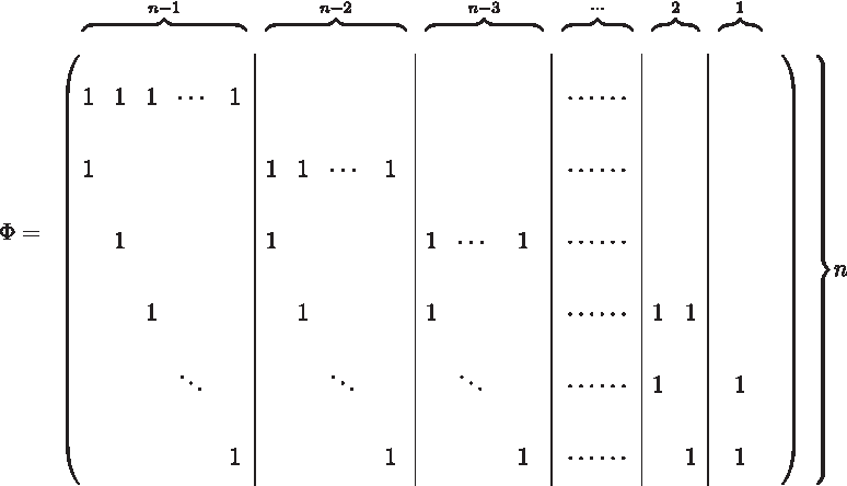
First, we vectorize the base-pairing probability matrix X = {x_ij}_1≤i<j≤n as \documentclass{aastex}\usepackage{amsbsy}\usepackage{amsfonts}\usepackage{amssymb}\usepackage{bm}\usepackage{mathrsfs}\usepackage{pifont}\usepackage{stmaryrd}\usepackage{textcomp}\usepackage{portland, xspace}\usepackage{amsmath, amsxtra}\pagestyle{empty}\DeclareMathSizes{10}{9}{7}{6}\begin{document} $$x = \{ x_s \} _{s = 1}^{n ( n - 1 ) / 2}$$ \end{document} where x_ij (i < j) corresponds to x_s with s = (2n−i)(i−1)/2 + (j−i). A = {a_ij}_1≤i<j≤n is also vectorized to \documentclass{aastex}\usepackage{amsbsy}\usepackage{amsfonts}\usepackage{amssymb}\usepackage{bm}\usepackage{mathrsfs}\usepackage{pifont}\usepackage{stmaryrd}\usepackage{textcomp}\usepackage{portland, xspace}\usepackage{amsmath, amsxtra}\pagestyle{empty}\DeclareMathSizes{10}{9}{7}{6}\begin{document} $$a = \{ a_s \} _{s = 1}^{n ( n - 1 ) / 2}$$ \end{document} . Second, we introduce the following n × n(n−1)/2 binary matrix.

where each blank in the matrix is equal to 0. It is easily seen that the ith element of Φx is equal to \documentclass{aastex}\usepackage{amsbsy}\usepackage{amsfonts}\usepackage{amssymb}\usepackage{bm}\usepackage{mathrsfs}\usepackage{pifont}\usepackage{stmaryrd}\usepackage{textcomp}\usepackage{portland, xspace}\usepackage{amsmath, amsxtra}\pagestyle{empty}\DeclareMathSizes{10}{9}{7}{6}\begin{document} $$\sum_{ ( k , l ) \in { \cal I}_i} x_{kl}$$ \end{document} . Problem 2 can, therefore, be recast as solving the optimization problem \documentclass{aastex}\usepackage{amsbsy}\usepackage{amsfonts}\usepackage{amssymb}\usepackage{bm}\usepackage{mathrsfs}\usepackage{pifont}\usepackage{stmaryrd}\usepackage{textcomp}\usepackage{portland, xspace}\usepackage{amsmath, amsxtra}\pagestyle{empty}\DeclareMathSizes{10}{9}{7}{6}\begin{document} \begin{align*} & \hat x = {\mathop{\rm argmin}_ x} \ f ( x; a ) \\ & {\rm where} \ f ( x;a ) : = D ( x , a ) = \sum_{s = 1}^{n ( n - 1 ) / 2} \left( x_{s} \log {x_{s}} - x_s \log {a_{s}} - x_s \right) \\ & \hbox{subject to} \underline{u}^(\varepsilon) \le \Phi x \le \overline{u}^{ ( \varepsilon ) } \ { \rm and } \ x \ge 0\end{align*} \end{document}

where \documentclass{aastex}\usepackage{amsbsy}\usepackage{amsfonts}\usepackage{amssymb}\usepackage{bm}\usepackage{mathrsfs}\usepackage{pifont}\usepackage{stmaryrd}\usepackage{textcomp}\usepackage{portland, xspace}\usepackage{amsmath, amsxtra}\pagestyle{empty}\DeclareMathSizes{10}{9}{7}{6}\begin{document} $$\underline{u}^{ ( \varepsilon ) } = \left( \underline{u}^{ ( \varepsilon ) } _i \right)$$ \end{document} and \documentclass{aastex}\usepackage{amsbsy}\usepackage{amsfonts}\usepackage{amssymb}\usepackage{bm}\usepackage{mathrsfs}\usepackage{pifont}\usepackage{stmaryrd}\usepackage{textcomp}\usepackage{portland, xspace}\usepackage{amsmath, amsxtra}\pagestyle{empty}\DeclareMathSizes{10}{9}{7}{6}\begin{document} $$\overline{u}^{ ( \varepsilon ) } = \left( \overline{u}^{ ( \varepsilon ) }_i \right)$$ \end{document} . Note that f is a kind of Bregman function (Bregman, 1967), and there is a unique generalized projection onto a hyperplane. By using Theorem 6.4.1 in Censor and Zenios (1997), the following iteration converges to the solution of Problem 2.

Initialization step:  Initialize x⁰ and z⁰ as follows. \documentclass{aastex}\usepackage{amsbsy}\usepackage{amsfonts}\usepackage{amssymb}\usepackage{bm}\usepackage{mathrsfs}\usepackage{pifont}\usepackage{stmaryrd}\usepackage{textcomp}\usepackage{portland, xspace}\usepackage{amsmath, amsxtra}\pagestyle{empty}\DeclareMathSizes{10}{9}{7}{6}\begin{document} \begin{align*} & x^0 \in U : = \left\{ x \mid x \ge 0 , \exists z \in {\mathbb R}^{n} \ { \rm s.t.} \ \nabla f ( x ) = - \Phi^T z \right\} \\ & \nabla f ( x^0 ) = - \Phi^T z^0\end{align*} \end{document}

Iteration step:  For \documentclass{aastex}\usepackage{amsbsy}\usepackage{amsfonts}\usepackage{amssymb}\usepackage{bm}\usepackage{mathrsfs}\usepackage{pifont}\usepackage{stmaryrd}\usepackage{textcomp}\usepackage{portland, xspace}\usepackage{amsmath, amsxtra}\pagestyle{empty}\DeclareMathSizes{10}{9}{7}{6}\begin{document} $$\nu = 0 , 1 , 2 , \ldots,$$ \end{document} \documentclass{aastex}\usepackage{amsbsy}\usepackage{amsfonts}\usepackage{amssymb}\usepackage{bm}\usepackage{mathrsfs}\usepackage{pifont}\usepackage{stmaryrd}\usepackage{textcomp}\usepackage{portland, xspace}\usepackage{amsmath, amsxtra}\pagestyle{empty}\DeclareMathSizes{10}{9}{7}{6}\begin{document} \begin{align*} & \nabla f ( x^{ \nu + 1} ) = \nabla f ( x^ \nu ) + c_v \phi^{i ( \nu ) } & \tag{6}\end{align*} \end{document} \documentclass{aastex}\usepackage{amsbsy}\usepackage{amsfonts}\usepackage{amssymb}\usepackage{bm}\usepackage{mathrsfs}\usepackage{pifont}\usepackage{stmaryrd}\usepackage{textcomp}\usepackage{portland, xspace}\usepackage{amsmath, amsxtra}\pagestyle{empty}\DeclareMathSizes{10}{9}{7}{6}\begin{document} \begin{align*} z^{ \nu + 1} = z^ \nu - c_ \nu e^{i ( \nu ) } \tag{7} \end{align*} \end{document} \documentclass{aastex}\usepackage{amsbsy}\usepackage{amsfonts}\usepackage{amssymb}\usepackage{bm}\usepackage{mathrsfs}\usepackage{pifont}\usepackage{stmaryrd}\usepackage{textcomp}\usepackage{portland, xspace}\usepackage{amsmath, amsxtra}\pagestyle{empty}\DeclareMathSizes{10}{9}{7}{6}\begin{document} \begin{align*} c_ \nu = \min ( z_{i ( \nu ) }^ \nu , \delta_ \nu , \gamma_ \nu ) \tag{8} \end{align*} \end{document}

where i(ν) = (ν mod n + 1), φ;ⁱ is the ith row vector of Φ and eⁱ is the ith unit vector in \documentclass{aastex}\usepackage{amsbsy}\usepackage{amsfonts}\usepackage{amssymb}\usepackage{bm}\usepackage{mathrsfs}\usepackage{pifont}\usepackage{stmaryrd}\usepackage{textcomp}\usepackage{portland, xspace}\usepackage{amsmath, amsxtra}\pagestyle{empty}\DeclareMathSizes{10}{9}{7}{6}\begin{document} $${\mathbb R}^n$$ \end{document} (i.e., the ith element of e is 1; 0 otherwise). In Equation (8), δ_ν and γ_ν are Lagrangian multipliers for the optimization problems \documentclass{aastex}\usepackage{amsbsy}\usepackage{amsfonts}\usepackage{amssymb}\usepackage{bm}\usepackage{mathrsfs}\usepackage{pifont}\usepackage{stmaryrd}\usepackage{textcomp}\usepackage{portland, xspace}\usepackage{amsmath, amsxtra}\pagestyle{empty}\DeclareMathSizes{10}{9}{7}{6}\begin{document} \begin{align*}{ \rm Minimize} \ f ( x; x^ \nu ) \ \hbox{subject to} \sum_{k} \Phi_{i ( \nu ) k} x_k = \underline{u}_{i ( \nu ) }^{ ( \varepsilon ) } \tag{9}\end{align*} \end{document}

and \documentclass{aastex}\usepackage{amsbsy}\usepackage{amsfonts}\usepackage{amssymb}\usepackage{bm}\usepackage{mathrsfs}\usepackage{pifont}\usepackage{stmaryrd}\usepackage{textcomp}\usepackage{portland, xspace}\usepackage{amsmath, amsxtra}\pagestyle{empty}\DeclareMathSizes{10}{9}{7}{6}\begin{document} \begin{align*}{ \rm Minimize} \ f ( x; x^ \nu ) \ \hbox{subject to} \sum_{k} \Phi_{i ( \nu ) k} x_k = \overline{u}_{i ( \nu ) }^{ ( \varepsilon ) } \tag{10}\end{align*} \end{document}

respectively, where Φ _ik is the (i,k)-element in the matrix Φ.

We will now prove that the steps given above correspond to Algorithm 2. In the initialization step, we set z⁰ = 0 and hence x⁰ = a. The Lagrangian for Equation (9) is defined as \documentclass{aastex}\usepackage{amsbsy}\usepackage{amsfonts}\usepackage{amssymb}\usepackage{bm}\usepackage{mathrsfs}\usepackage{pifont}\usepackage{stmaryrd}\usepackage{textcomp}\usepackage{portland, xspace}\usepackage{amsmath, amsxtra}\pagestyle{empty}\DeclareMathSizes{10}{9}{7}{6}\begin{document} \begin{align*}L ( x , \gamma ) = \sum_s x_{s} ( \log x_s - \log x_s^ \nu - 1 ) - \delta_ \nu \left( \sum_{s} \Phi_{i ( \nu ) s} x_{s} - \underline{u}_{i ( \nu ) }^{ ( \varepsilon ) } \right). \tag{11}\end{align*} \end{document}

According to the KKT conditions (Kuhn and Tucker, 1951), the equations \documentclass{aastex}\usepackage{amsbsy}\usepackage{amsfonts}\usepackage{amssymb}\usepackage{bm}\usepackage{mathrsfs}\usepackage{pifont}\usepackage{stmaryrd}\usepackage{textcomp}\usepackage{portland, xspace}\usepackage{amsmath, amsxtra}\pagestyle{empty}\DeclareMathSizes{10}{9}{7}{6}\begin{document} \begin{align*} \frac { \partial L } { \partial x_ { s } } = 0 \ ({\rm for \ all} \ s) \ {\rm and} \ \frac { \partial L } { \partial \delta_ \nu } = 0\end{align*} \end{document}

are satisfied. Then, \documentclass{aastex}\usepackage{amsbsy}\usepackage{amsfonts}\usepackage{amssymb}\usepackage{bm}\usepackage{mathrsfs}\usepackage{pifont}\usepackage{stmaryrd}\usepackage{textcomp}\usepackage{portland, xspace}\usepackage{amsmath, amsxtra}\pagestyle{empty}\DeclareMathSizes{10}{9}{7}{6}\begin{document} \begin{align*} \frac { \partial L } { \partial x_ { s } } = \log x_ { s } - \log x_ { s } ^ { \nu } - \delta_ \nu \Phi_ { i ( \nu ) s } = 0 ,\end{align*} \end{document}

leads to \documentclass{aastex}\usepackage{amsbsy}\usepackage{amsfonts}\usepackage{amssymb}\usepackage{bm}\usepackage{mathrsfs}\usepackage{pifont}\usepackage{stmaryrd}\usepackage{textcomp}\usepackage{portland, xspace}\usepackage{amsmath, amsxtra}\pagestyle{empty}\DeclareMathSizes{10}{9}{7}{6}\begin{document} \begin{align*}x_{s} = x_{s}^{ \nu} \exp \left( \delta_ \nu \Phi_{i ( \nu ) s} \right). \tag{12}\end{align*} \end{document}

By substituting Equation (12) into Equation (11), we obtain \documentclass{aastex}\usepackage{amsbsy}\usepackage{amsfonts}\usepackage{amssymb}\usepackage{bm}\usepackage{mathrsfs}\usepackage{pifont}\usepackage{stmaryrd}\usepackage{textcomp}\usepackage{portland, xspace}\usepackage{amsmath, amsxtra}\pagestyle{empty}\DeclareMathSizes{10}{9}{7}{6}\begin{document} \begin{align*}L = - \sum_{s} x_{s}^ \nu \exp ( \delta_ \nu \Phi_{i ( \nu ) s} ) + \delta_ \nu \underline{u}_i^{ ( \varepsilon ) }. \tag{13}\end{align*} \end{document}

Differentiating Equation (13) with respect to δ_ν and setting the result equal to 0 gives \documentclass{aastex}\usepackage{amsbsy}\usepackage{amsfonts}\usepackage{amssymb}\usepackage{bm}\usepackage{mathrsfs}\usepackage{pifont}\usepackage{stmaryrd}\usepackage{textcomp}\usepackage{portland, xspace}\usepackage{amsmath, amsxtra}\pagestyle{empty}\DeclareMathSizes{10}{9}{7}{6}\begin{document} \begin{align*} \frac {\partial L} {\partial \delta_ \nu} = \sum_ {s} \Phi_ { i ( \nu ) s } x_ { s } ^ \nu \exp ( \delta_ \nu \Phi_ { i ( \nu ) s } ) - \underline { u } _i^ { ( \varepsilon ) } = 0\end{align*} \end{document}

which leads to \documentclass{aastex}\usepackage{amsbsy}\usepackage{amsfonts}\usepackage{amssymb}\usepackage{bm}\usepackage{mathrsfs}\usepackage{pifont}\usepackage{stmaryrd}\usepackage{textcomp}\usepackage{portland, xspace}\usepackage{amsmath, amsxtra}\pagestyle{empty}\DeclareMathSizes{10}{9}{7}{6}\begin{document} \begin{align*}\exp ( \delta_ \nu ) = \frac {\overline {u} _i^ {(\varepsilon)}} {\sum_ {s: \Phi_ {i (\nu) s} = 1} x_s^ \nu} .\end{align*} \end{document}

Similarly, we obtain \documentclass{aastex}\usepackage{amsbsy}\usepackage{amsfonts}\usepackage{amssymb}\usepackage{bm}\usepackage{mathrsfs}\usepackage{pifont}\usepackage{stmaryrd}\usepackage{textcomp}\usepackage{portland, xspace}\usepackage{amsmath, amsxtra}\pagestyle{empty}\DeclareMathSizes{10}{9}{7}{6}\begin{document} \begin{align*}\exp ( \gamma_ \nu ) = \frac { \underline { u } _i^ { ( \varepsilon ) } } { \sum_ { s: \Phi_ { i ( \nu ) s } = 1 } x_s^ \nu } .\end{align*} \end{document}

By taking exponentials of Equations (7) and (8), we have \documentclass{aastex}\usepackage{amsbsy}\usepackage{amsfonts}\usepackage{amssymb}\usepackage{bm}\usepackage{mathrsfs}\usepackage{pifont}\usepackage{stmaryrd}\usepackage{textcomp}\usepackage{portland, xspace}\usepackage{amsmath, amsxtra}\pagestyle{empty}\DeclareMathSizes{10}{9}{7}{6}\begin{document} \begin{align*}\exp ( z^ { \nu + 1 } _ { i ( \nu ) } ) = \frac { \exp ( z^ \nu_ { i ( \nu ) } ) } { \exp ( c_ \nu ) } \tag { 14 } \end{align*} \end{document} \documentclass{aastex}\usepackage{amsbsy}\usepackage{amsfonts}\usepackage{amssymb}\usepackage{bm}\usepackage{mathrsfs}\usepackage{pifont}\usepackage{stmaryrd}\usepackage{textcomp}\usepackage{portland, xspace}\usepackage{amsmath, amsxtra}\pagestyle{empty}\DeclareMathSizes{10}{9}{7}{6}\begin{document} \begin{align*}\exp ( c_ \nu ) = { \rm median} \left( \exp ( z_{i ( \nu ) }^ \nu ) , \exp ( \delta_ \nu ) , \exp ( \gamma_ \nu ) \right) \tag{15}\end{align*} \end{document}

respectively. Equations (14) and (15) lead to lines 26 and 22 in Algorithm 2, respectively. Finally, \documentclass{aastex}\usepackage{amsbsy}\usepackage{amsfonts}\usepackage{amssymb}\usepackage{bm}\usepackage{mathrsfs}\usepackage{pifont}\usepackage{stmaryrd}\usepackage{textcomp}\usepackage{portland, xspace}\usepackage{amsmath, amsxtra}\pagestyle{empty}\DeclareMathSizes{10}{9}{7}{6}\begin{document} \begin{align*}x_s^{ \nu + 1} = x_s^ \nu \exp \left( c_ \nu \phi_s^{i ( \nu ) } \right) = x_s^ \nu \exp \left( c_ \nu \right) \exp \left( \phi_s^{i ( \nu ) } \right) \tag{16}\end{align*} \end{document}

leads to line 24 in Algorithm 2, and the proof is finished. ■

4. Computational Experiments

We have implemented a Perl script for updating a given initial base-pairing probability matrix in order to satisfy marginal constraints (Algorithms 1 and 2). For the updated base-pairing probability matrix, the γ-centroid estimator (Hamada et al., 2009b) was employed to predict a secondary structure from the BPPM. More specifically, we maximize the sum of the (updated) base-pairing probabilities for base pairs in the predicted secondary structure, in which base pairs whose probability is larger than 1/(γ + 1) are allowed to form a base pair (Hamada et al., 2009b). The γ is a parameter used to adjust the balance between sensitivity and positive predictive value of predicted base-pairs (a smaller γ produces fewer base pairs). CentroidFold software (http://ncrna.org/software/centroidfold/download/), which is an implementation of the γ-centroid estimator, was utilized. In the following experiments, the initial BPPM (A in Algorithms 1 and 2) is given by computational methods—either the Boltzmann likelihood (BL) model (Andronescu et al., 2010) or the CONTRAfold model (Do et al., 2006), both of which are implemented in the CentroidFold software.

To confirm that our algorithm works correctly, we first conducted computational experiments with perfect constraints. Here, the constraints q (in Definition 4) are given according to the reference secondary structure: q_i = 1 when the base at position i forms a base pair in the reference secondary structure and q_i = 0 otherwise. As a benchmark dataset, we used the “S151 Rfam dataset,” which has been employed in many studies (Do et al., 2006; Hamada et al., 2011a).

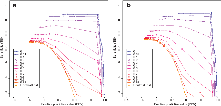
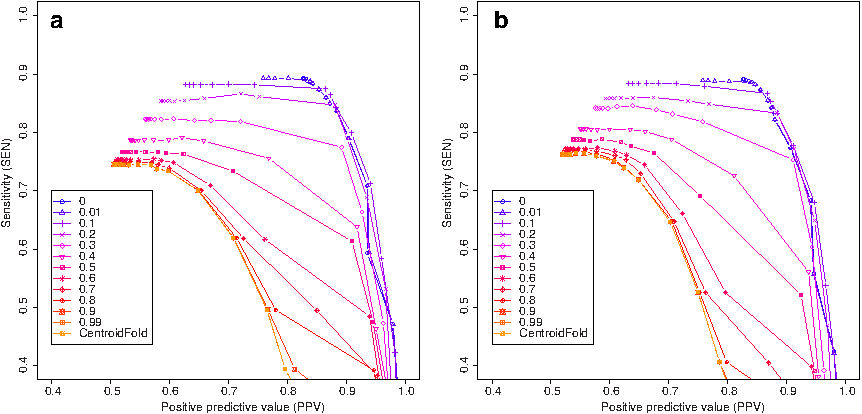
The results of the first experiment are shown in Figure 1. As performance measures, we used the sensitivity (SEN) and positive predictive value (PPV): SEN = TP/(TP + FN) and PPV = TP/(TP + FP) where TP, FP, and FN are the numbers of true-positive base pairs, false-positive base pairs, and false-negative base pairs, respectively. We computed those values for each predicted secondary structure only once for the entire dataset. In the γ-centroid estimator, 17 γ values, \documentclass{aastex}\usepackage{amsbsy}\usepackage{amsfonts}\usepackage{amssymb}\usepackage{bm}\usepackage{mathrsfs}\usepackage{pifont}\usepackage{stmaryrd}\usepackage{textcomp}\usepackage{portland, xspace}\usepackage{amsmath, amsxtra}\pagestyle{empty}\DeclareMathSizes{10}{9}{7}{6}\begin{document} $$\gamma \in \{ 2^k: - 5 \le k \le 10 , k \in {\mathbb Z} \} \cup \{ 6 \} $$ \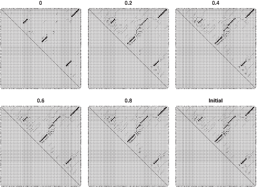end{document} , were used to draw sensitivity-PPV curves. For each probabilistic model for RNA secondary structures, when ɛ is close to 1, the performance approaches the case in which secondary structure is predicted only from the initial base-pairing probability matrix (i.e., the performance of the original CentroidFold software), because the initial BPPM itself satisfies the marginal constraint (Eq. 4) when ɛ is large. Examples of updated base-pairing probability matrices for every ɛ value are shown in Figure 2; tRNA sequences were utilized in the experiments. Table 1 shows that the computational time is shorter for larger ɛ, because the number of iterations is smaller for lager epsilon. On the other hand, the computational time for ɛ = 0 is slightly faster than the case of ɛ = 0.01, because, in the former case, the simpler Algorithm 1 is used rather than Algorithm 2.

OPEN IN VIEWER

FIG. 1.

Benchmark experiments for perfect constraints for various ɛ values (the relaxation parameter in Problem 2). The γ-centroid estimators (Hamada et al., 2009b) are used when estimating secondary structures from the updated base-pairing probability matrix. We utilized the S151 Rfam dataset in this experiment, and constraints are given according to reference secondary structures. Initial base-pairing probability matrices are computed using (a) the BL model (Andronescu et al., 2010) and (b) the CONTRAfold model (Do et al., 2006).

OPEN IN VIEWER

FIG. 2.

Updated base-pairing probability matrices of a tRNA sequence (RF00005) for ɛ = 0, 0.2, 0.4, 0.6, 0.8. Perfect constraints were utilized in this example. The bottom and rightmost figure (labeled “Initial”) is the initial base-pairing probability matrix (i.e., A in Algorithms 1 and 2).

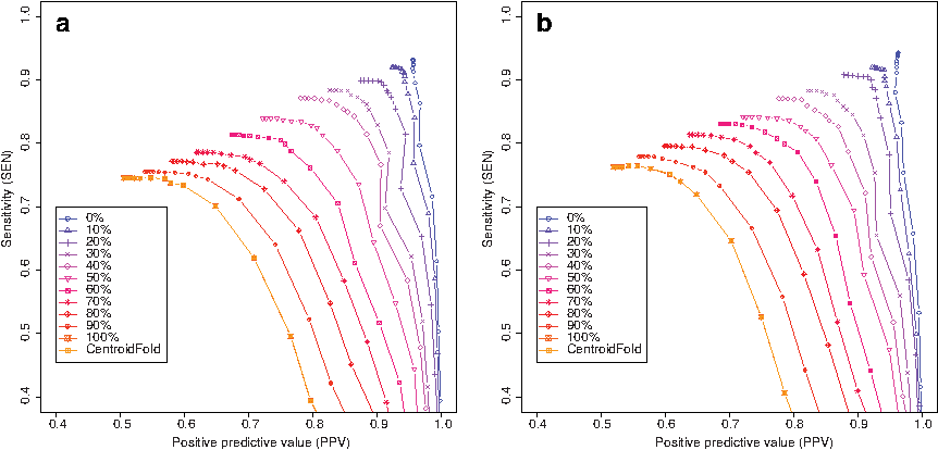
Second, we conducted experiments using marginal constraints with missing data, where missing data is simulated in the perfect constraints described above. The ratio of missing positions varies from 0% to 100% in 10% steps. Figure 3 shows the results, indicating that the performance gradually approaches that of the original CentroidFold as the proportion of missing data increases.

OPEN IN VIEWER

FIG. 3.

Benchmark experiments for constraints including missing data, which are simulated by inserting missing values in the perfect constraints. The ratio of missing positions varies 0% to 100% in 10% steps. The γ-centroid estimators (Hamada et al., 2009b) are used when estimating secondary structures from the updated base-pairing probability matrix. We utilized the S151 Rfam dataset in this experiment and, constraints are given according to reference secondary structures. Initial base-pairing probability matrices are computed using (a) the BL model and (b) the CONTRAfold model.

Third, we conducted experiments for marginal probability constraints with noise. In this dataset, we simulated uniform noise of 10% for positions in loop regions and 30% noise in base-pair regions, with respect to perfect constraints. Figure 4 shows the results. This indicates that the performance for ɛ = 0 was worse than that for ɛ ≠ 0 in a part of sensitivity-PPV curve, which indicates that a non-zero ɛ value could have the potential to improve the prediction accuracy when constraints include noise.

OPEN IN VIEWER

FIG. 4.

Benchmark experiments for constraints with noise using various values of ɛ (the relaxation parameter). We simulated uniform noise of 10% for positions in loop regions and 30% noise in base-pair regions, with respect to perfect constraints. The γ-centroid estimators (Hamada et al., 2009b) are used when estimating secondary structures from updated base-pairing probability. We utilized the S151 Rfam dataset in this experiment, and constraints are given according to reference secondary structures. Initial base-pairing probability matrices are computed using (a) the BL model and (b) the CONTRAfold model.

5. Discussion

In this study, we have introduced a simple algorithm to transform a given initial base-pairing probability matrix (BPPM) into a new one that satisfies marginal probability constraints, by finding a BPPM that is “near” the initial one (where nearness is measured by the Kullback-Leibler distance). Although, strictly speaking, there is no guarantee that there exists a probability distribution on \documentclass{aastex}\usepackage{amsbsy}\usepackage{amsfonts}\usepackage{amssymb}\usepackage{bm}\usepackage{mathrsfs}\usepackage{pifont}\usepackage{stmaryrd}\usepackage{textcomp}\usepackage{portland, xspace}\usepackage{amsmath, amsxtra}\pagestyle{empty}\DeclareMathSizes{10}{9}{7}{6}\begin{document} $${\cal S}$$ \end{document} (x) that produces the updated matrix, computational experiments showed that our algorithm is robust to missing data (cf. Fig. 3) and noise (cf. Fig. 4).

The proposed algorithms are applicable in any situation in which the base-pairing probability matrix of an RNA sequence can be found. This matrix can be computed by any algorithm, such as RNAfold (Hofacker et al., 1994), RNAstructure (Mathews et al., 1999) or CONTRAfold (Do et al., 2006). Notably, we also use our method with base-pairing probability matrices computed by Rfold (Kiryu et al., 2008) or RNAplfold (Bernhart et al., 2006) (these algorithms can restrict the maximum number of base pairs). This enables us to incorporate experimental data of very long sequences, such as the long transcriptome appearing in Underwood et al. (2010). It should also be emphasized that, by using an updated BPPM, many RNA informatics algorithms that internally employ BPPMs can be improved without modifying the algorithms themselves.

Converting experimental information given by SHAPE (Low and Weeks, 2010), PARS (Kertesz et al., 2010), and FragSeq (Underwood et al., 2010) technologies into marginal probability constraints (Definition 4) is not trivial. Some recent studies suggest that the experimental data include relatively large amount of noise, which can not be neglected (Kladwang et al., 2011). We believe that our algorithm including ɛ-relaxation is useful for those cases (cf. Fig. 4). In this article, we have mainly focused on the algorithms. Extensive computational experiments (using SHAPE, PARS, and FragSeq) will be undertaken in future work. It would be also interesting to investigate other ways of characterizing the distance (divergence) between BPPMs as alternatives to using the Kullback-Leibler distance (Amari and Nagaoka, 2000).

References

1.
AmariS., NagaokaH.2000. Methods of Information Geometry. Translations of Mathematical Monographs series, 191. Oxford University Press: New York.
AndronescuM., CondonA., HoosH.H.et al.2010. Computational approaches for RNA energy parameter estimation. RNA, 16:2304–2318.
4.
BernhartS.H., HofackerI.L., StadlerP.F.2006. Local RNA base pairing probabilities in large sequences. Bioinformatics, 22:614–615.
5.
BregmanL.1967. The relaxation method of finding the common points of convex sets and its application to the solution of problems in convex programming. USSR Computational Mathematics and Mathematical Physics, 7:200–217.
6.
CarvalhoL., LawrenceC.2008. Centroid estimation in discrete high-dimensional spaces with applications in biology. Proc. Natl. Acad. Sci. U.S.A., 105:3209–3214.
7.
CensorY.A., ZeniosS.A.1997. Parallel Optimization: Theory, Algorithms and Applications. Oxford University Press: New York.
8.
DeiganK.E., LiT.W., MathewsD.H.et al.2009. Accurate SHAPE-directed RNA structure determination. Proc. Natl. Acad. Sci. U.S.A., 106:97–102.
HamadaM., SatoK., KiryuH.et al.2009a. CentroidAlign: fast and accurate aligner for structured RNAs by maximizing expected sum-of-pairs score. Bioinformatics, 25:3236–3243.
14.
HamadaM., KiryuH., SatoK.et al.2009b. Prediction of RNA secondary structure using generalized centroid estimators. Bioinformatics, 25:465–473.
15.
HamadaM., YamadaK., SatoK.et al.2011a. CentroidHomfold-LAST: accurate prediction of RNA secondary structure using automatically collected homologous sequences. Nucleic Acids Res., 39:W100–106.
HamadaM., SatoK., AsaiK.2011c. Improving the accuracy of predicting secondary structure for aligned RNA sequences. Nucleic Acids Res., 39:393–402.
18.
HofackerI., FontanaW., StadlerP.et al.1994. Fast folding and comparison of RNA secondary structures. Monatsh. Chem., 125:167–188.
19.
HofackerI.L., BernhartS.H.F., StadlerP.F.2004. Alignment of RNA base pairing probability matrices. Bioinformatics, 20:2222–2227.
20.
JanssenS., SchudomaC., StegerG., GiegerichR.2011. Lost in folding space? Comparing four variants of the thermodynamic model for RNA secondary structure prediction. BMC Bioinformatics, 12:429.
21.
KatoY., SatoK., HamadaM.et al.2010. RactIP: fast and accurate prediction of RNA-RNA interaction using integer programming. Bioinformatics, 26:i460–466.
22.
KatohK., TohH.2008. Improved accuracy of multiple ncRNA alignment by incorporating structural information into a MAFFT-based framework. BMC Bioinformatics, 9:212.
23.
KerteszM., WanY., MazorE.et al.2010. Genome-wide measurement of RNA secondary structure in yeast. Nature, 467:103–107.
24.
KiryuH., KinT., AsaiK.2008. Rfold: an exact algorithm for computing local base pairing probabilities. Bioinformatics, 24:367–373.
25.
KladwangW., VanLangC.C., CorderoP., DasR.2011. Understanding the errors of SHAPE-directed RNA structure modeling. Biochemistry, 50:8049–8056.
26.
KuhnH., TuckerA.1951. Nonlinear programming, 481–492. NeymanJ.Proceedings of the Second Berkeley Symposium on Mathematical Statistics and Probability, University of California Press, Berkeley, California.
27.
LeontisN., WesthofE.2012. RNA 3D Structure Analysis and Prediction (Nucleic Acids and Molecular Biology)Springer: New York.
MathewsD.H., SabinaJ., ZukerM., TurnerD.H.1999. Expanded sequence dependence of thermodynamic parameters improves prediction of RNA secondary structure. J. Mol. Biol., 288:911–940.
31.
McCaskillJ.S.1990. The equilibrium partition function and base pair binding probabilities for RNA secondary structure. Biopolymers, 29:1105–1119.
32.
MoriokaR., TsudaK.2011. Information geometry of input-output tables. Technical note in IBISML, 110:161–167(in Japanese).
33.
NovikovaI.V., HennellyS.P., SanbonmatsuK.Y.2012. Structural architecture of the human long non-coding RNA, steroid receptor RNA activator. Nucleic Acids Res, 40:5034–5051.
34.
PangP.S., ElazarM., PhamE.A., GlennJ.S.2011. Simplified RNA secondary structure mapping by automation of SHAPE data analysis. Nucleic Acids Res., 39:e151.
35.
QuarrierS., MartinJ.S., Davis-NeulanderL.et al.2010. Evaluation of the information content of RNA structure mapping data for secondary structure prediction. RNA, 16:1108–1117.
36.
RivasE., LangR., EddyS.R.2012. A range of complex probabilistic models for RNA secondary structure prediction that includes the nearest-neighbor model and more. RNA, 18:193–212.
37.
SahraeianS.M., YoonB.J.2011. PicXAA-R: efficient structural alignment of multiple RNA sequences using a greedy approach. BMC Bioinformatics, 12,Suppl 1:S38.
38.
SatoK., HamadaM., MituyamaT.et al.2009. A non-parametric bayesian approach for predicting RNA secondary structures. Proceedings of the 9th International Conference on Algorithms in Bioinformatics, 286–297.
39.
SatoK., KatoY., HamadaM.et al.2011. IPknot: fast and accurate prediction of RNA secondary structures with pseudoknots using integer programming. Bioinformatics, 27:i85–i93.
40.
SeemannS., GorodkinJ., BackofenR.2008. Unifying evolutionary and thermodynamic information for RNA folding of multiple alignments. Nucleic Acids Res., 36:6355–6362.
41.
SeemannS.E., RichterA.S., GesellT.et al.2011. PETcofold: predicting conserved interactions and structures of two multiple alignments of RNA sequences. Bioinformatics, 27:211–219.
42.
TeraiG., KomoriT., AsaiK., KinT.2007. miRRim: a novel system to find conserved miRNAs with high sensitivity and specificity. RNA, 13:2081–2090.
WanY., KerteszM., SpitaleR.C.et al.2011. Understanding the transcriptome through RNA structure. Nat. Rev. Genet., 12:641–655.
45.
WashietlS., HofackerI.L., StadlerP.F., KellisM.2012. RNA folding with soft constraints: reconciliation of probing data and thermodynamic secondary structure prediction. Nucleic Acids Res, 40:4261–4272.
46.
WattsJ.M., DangK.K., GorelickR.J.et al.2009. Architecture and secondary structure of an entire HIV-1 RNA genome. Nature, 460:711–716.
47.
WeiD., AlpertL.V., LawrenceC.E.2011. Rnag: A new gibbs sampler for predicting RNA secondary structure for unaligned sequences. Bioinformatics, 27:2486–2493.