Live Phylogeny

1. Introduction

Phylogeny is a core problem in computational molecular biology. Starting with a set of taxonomic objects, the problem is to reconstruct their evolutionary history. The result is a tree in which taxonomic objects are leaves and hypothetical ancestors are added as internal nodes (Felsenstein, 2004; Gusfield, 1997; Setubal and Meidanis, 1997).

This article introduces the problem of live phylogeny, where a phylogenetic tree must be reconstructed but ancestors are present among the input taxonomic objects. This way, internal nodes in the resulting tree may be either actual objects or hypothetical ancestors. Real-world applications are the analysis of viral populations or other fast-evolving organisms (Castro-Nallar et al., 2012; Gojobori et al., 1990), and the phylogenetic analysis of nonbiological objects, such as documents, images, or relational database entries (Cuadros et al., 2007; Paiva et al., 2011). We present the problem both for distances and characters. For distances, we investigated the case in which the matrices are additive. For characters, we considered absence of convergence and reversals. We give polynomial algorithms for both problems. To our best knowledge, this is the first characterization of these problems in phylogeny.

This article is organized as follows. Section 2 is devoted to the distance-based live phylogen problem, and Section 3 to the character states live phylogeny problem. In Section 4, we present some conclusions.

2. Distance-Based Live Phylogeny

In the distance-based phylogeny problem, one wants to build an unrooted, weighted tree in which the distances among leaves are equal to the distances given in a distance matrix. The input is an n × n matrix M, where M_i,j is the distance between objects o_i and o_j. The output is a tree in which each leaf represents an object and all internal nodes have degree 3. When it is possible to build such a tree, then the distances in M are said to be additive.

It is known that if M is additive, then a polynomial algorithm solves the problem (Setubal and Meidanis, 1997). It is also known that a distance matrix M is additive if it is a metric space and respects the four-point condition, which states that given any four objects, it is possible to label them as o_i, o_j, o_k, o_l, such that \documentclass{aastex}\usepackage{amsbsy}\usepackage{amsfonts}\usepackage{amssymb}\usepackage{bm}\usepackage{mathrsfs}\usepackage{pifont}\usepackage{stmaryrd}\usepackage{textcomp}\usepackage{portland, xspace}\usepackage{amsmath, amsxtra}\pagestyle{empty}\DeclareMathSizes{10}{9}{7}{6}\begin{document} \begin{align*}M_{i , j} + M_{k , l} = M_{i , k} + M_{j , l} \ge M_{i , l} + M_{j , k}.\end{align*} \end{document}

By the other side, minimizing the nonadditivity deviation is an NP-hard problem (Day, 1987).

In distance-based live phylogeny, objects may be represented by internal nodes of the tree as well, in order to reflect living ancestors in the set of objects.

Formally, let Mⁿ be a square matrix of order n, representing objects \documentclass{aastex}\usepackage{amsbsy}\usepackage{amsfonts}\usepackage{amssymb}\usepackage{bm}\usepackage{mathrsfs}\usepackage{pifont}\usepackage{stmaryrd}\usepackage{textcomp}\usepackage{portland, xspace}\usepackage{amsmath, amsxtra}\pagestyle{empty}\DeclareMathSizes{10}{9}{7}{6}\begin{document} $$o_1 \ldots o_n$$ \end{document} , where \documentclass{aastex}\usepackage{amsbsy}\usepackage{amsfonts}\usepackage{amssymb}\usepackage{bm}\usepackage{mathrsfs}\usepackage{pifont}\usepackage{stmaryrd}\usepackage{textcomp}\usepackage{portland, xspace}\usepackage{amsmath, amsxtra}\pagestyle{empty}\DeclareMathSizes{10}{9}{7}{6}\begin{document} $$M_{i , j}^n \in {\mathbb R}$$ \end{document} is the distance between objects o_i and o_j. Let Tⁿ be a weighted, unrooted tree. Tⁿ is a live phylogeny for Mⁿ if Tⁿ is compatible with Mⁿ. A tree Tⁿ is compatible with a matrix Mⁿ, denoted Tⁿ ∼ Mⁿ, if

• each leaf of Tⁿ is labeled with one object,

Internal nodes are called ancestors. An ancestor is live if it is labeled o_i, for some i, and is hypothetical otherwise.

The distance-based live phylogeny problem is, given Mⁿ additive, to build a live phylogeny Tⁿ. Here we provide a constructive proof that a live phylogeny can always be built from an additive matrix Mⁿ.

Theorem 1. Let M^k additive and T^k be such that M^k ∼ T^k. Let M^k+1 additive be M^k with a new object o_k+1 distinct from every o_i, 1 ≤ i ≤ k, added to it. We can add o_k+1 to T^k, obtaining T^k+1 ∼ M^k+1.

Proof: By induction on k ≥ 2.

Basis

Suppose k = 2 and let x, y be the only two leaves of T². Let z = o₃ be the new node to be added to T², obtaining T³. We have the four following possible cases, based on the relationships among x, y, z in T³.

Case 1: \documentclass{aastex}\usepackage{amsbsy}\usepackage{amsfonts}\usepackage{amssymb}\usepackage{bm}\usepackage{mathrsfs}\usepackage{pifont}\usepackage{stmaryrd}\usepackage{textcomp}\usepackage{portland, xspace}\usepackage{amsmath, amsxtra}\pagestyle{empty}\DeclareMathSizes{10}{9}{7}{6}\begin{document} $$M_{xy}^3 = M_{xz}^3 + M_{zy}^3$$ \end{document} . In this case, add z to the edge (x, y) of T² in such way that \documentclass{aastex}\usepackage{amsbsy}\usepackage{amsfonts}\usepackage{amssymb}\usepackage{bm}\usepackage{mathrsfs}\usepackage{pifont}\usepackage{stmaryrd}\usepackage{textcomp}\usepackage{portland, xspace}\usepackage{amsmath, amsxtra}\pagestyle{empty}\DeclareMathSizes{10}{9}{7}{6}\begin{document} $$d_{xz}^3 = M_{xz}^3$$ \end{document} and \documentclass{aastex}\usepackage{amsbsy}\usepackage{amsfonts}\usepackage{amssymb}\usepackage{bm}\usepackage{mathrsfs}\usepackage{pifont}\usepackage{stmaryrd}\usepackage{textcomp}\usepackage{portland, xspace}\usepackage{amsmath, amsxtra}\pagestyle{empty}\DeclareMathSizes{10}{9}{7}{6}\begin{document} $$d_{zy}^3 = M_{zy}^3$$ \end{document} , obtaining T³ (Fig. 1).

OPEN IN VIEWER

FIG. 1.

In Case 1, node z is a live ancestor of x and y.

Case 2: \documentclass{aastex}\usepackage{amsbsy}\usepackage{amsfonts}\usepackage{amssymb}\usepackage{bm}\usepackage{mathrsfs}\usepackage{pifont}\usepackage{stmaryrd}\usepackage{textcomp}\usepackage{portland, xspace}\usepackage{amsmath, amsxtra}\pagestyle{empty}\DeclareMathSizes{10}{9}{7}{6}\begin{document} $$M_{xz}^3 = M_{xy}^3 + M_{yz}^3$$ \end{document} . In this case, add a new edge (y, z) to T² such that \documentclass{aastex}\usepackage{amsbsy}\usepackage{amsfonts}\usepackage{amssymb}\usepackage{bm}\usepackage{mathrsfs}\usepackage{pifont}\usepackage{stmaryrd}\usepackage{textcomp}\usepackage{portland, xspace}\usepackage{amsmath, amsxtra}\pagestyle{empty}\DeclareMathSizes{10}{9}{7}{6}\begin{document} $$d_{yz}^3 = M_{yz}^3$$ \end{document} and \documentclass{aastex}\usepackage{amsbsy}\usepackage{amsfonts}\usepackage{amssymb}\usepackage{bm}\usepackage{mathrsfs}\usepackage{pifont}\usepackage{stmaryrd}\usepackage{textcomp}\usepackage{portland, xspace}\usepackage{amsmath, amsxtra}\pagestyle{empty}\DeclareMathSizes{10}{9}{7}{6}\begin{document} $$d_{xz}^3 = M_{xz}^3$$ \end{document} , obtaining T³ (Fig. 2).

OPEN IN VIEWER

FIG. 2.

In Case 2, node y became a live ancestor of x and z.

Case 3: \documentclass{aastex}\usepackage{amsbsy}\usepackage{amsfonts}\usepackage{amssymb}\usepackage{bm}\usepackage{mathrsfs}\usepackage{pifont}\usepackage{stmaryrd}\usepackage{textcomp}\usepackage{portland, xspace}\usepackage{amsmath, amsxtra}\pagestyle{empty}\DeclareMathSizes{10}{9}{7}{6}\begin{document} $$M_{yz}^3 = M_{xy}^3 + M_{xz}^3$$ \end{document} . In this case, add a new edge (z, x) to T² such that \documentclass{aastex}\usepackage{amsbsy}\usepackage{amsfonts}\usepackage{amssymb}\usepackage{bm}\usepackage{mathrsfs}\usepackage{pifont}\usepackage{stmaryrd}\usepackage{textcomp}\usepackage{portland, xspace}\usepackage{amsmath, amsxtra}\pagestyle{empty}\DeclareMathSizes{10}{9}{7}{6}\begin{document} $$d_{zx}^3 = M_{zx}^3$$ \end{document} and \documentclass{aastex}\usepackage{amsbsy}\usepackage{amsfonts}\usepackage{amssymb}\usepackage{bm}\usepackage{mathrsfs}\usepackage{pifont}\usepackage{stmaryrd}\usepackage{textcomp}\usepackage{portland, xspace}\usepackage{amsmath, amsxtra}\pagestyle{empty}\DeclareMathSizes{10}{9}{7}{6}\begin{document} $$d_{yz}^3 = M_{zy}^3$$ \end{document} , obtaining T³ (Fig. 3).

OPEN IN VIEWER

FIG. 3.

In Case 3, node x becomes a live ancestor of y and z.

Notice that Cases 1, 2, and 3 are exclusive, otherwise z = x or z = y, and we are assuming that all objects are distinct.

Case 4: When none of the previous cases happens, and because of triangle inequality, we have \documentclass{aastex}\usepackage{amsbsy}\usepackage{amsfonts}\usepackage{amssymb}\usepackage{bm}\usepackage{mathrsfs}\usepackage{pifont}\usepackage{stmaryrd}\usepackage{textcomp}\usepackage{portland, xspace}\usepackage{amsmath, amsxtra}\pagestyle{empty}\DeclareMathSizes{10}{9}{7}{6}\begin{document} \begin{align*}d_{xz}^3 + d_{zy}^3 > d_{xy}^3 , d_{xy}^3 + d_{yz}^3 > d_{xz}^3 , d_{xy}^3 + d_{xz}^3 > d_{yz}^3.\end{align*} \end{document}

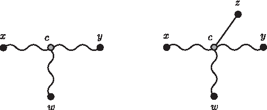
In this case, add a new internal node c on the edge (x, y) and connect it to z obtaining T³, such that \documentclass{aastex}\usepackage{amsbsy}\usepackage{amsfonts}\usepackage{amssymb}\usepackage{bm}\usepackage{mathrsfs}\usepackage{pifont}\usepackage{stmaryrd}\usepackage{textcomp}\usepackage{portland, xspace}\usepackage{amsmath, amsxtra}\pagestyle{empty}\DeclareMathSizes{10}{9}{7}{6}\begin{document} \begin{align*}d_ {xc} ^3 = \frac {M_ {xy} ^3 + M_ {xz} ^3 - M_ {yz} ^3} {2} > 0 , \ d_ {yc} ^3 = \frac {M_ {xy} ^3 + M_ {yz} ^3 - M_ {xz} ^3} {2} > 0 , \ d_ {zc} ^3 = \frac {M_ {xz} ^3 + M_ {yz} ^3 - M_ {xy} ^3} {2} > 0\end{align*} \end{document}

(Fig. 4). This completes the basis.

OPEN IN VIEWER

FIG. 4.

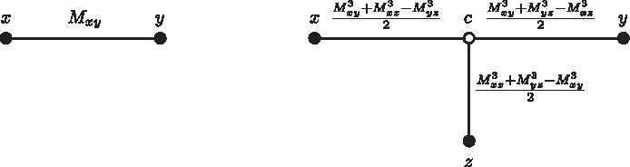
In Case 4, there is a hypothetical ancestor c of x, y, and z.

Inductive step

Suppose that T^k ∼ M^k, k ≥ 3. We will show how to add a new node z to T^k, obtaining T^k+1 ∼ M^k+1. Let x, y be any two leaves of T^k. Again, we have four possibilities.

In favor of a clearer notation, we denote M^k+1 by M, d^k+1 by d, and the only path connecting any nodes x and y in a tree by (x, y)-path.

Case i: M_xz + M_zy = M_xy. In this case, z must be inserted in the (x, y)-path, such that d_xz = M_xz and d_zy = M_zy. It is exactly the same situation shown in Figure 1, except that now we are handling an (x, y)-path, not necessarily an edge (x, y).

Let us suppose there is no node in the position where z has been added. The case in which there is already such a node will be seen soon.

We need to show that d_zw = M_zw for any node w ≠ x, y. Suppose that w is not in (x, y)-path, but it is connected to it by a node c in the (z, y)-path (Fig. 5). The case where c is in (x, z)-path is analogous.

OPEN IN VIEWER

FIG. 5.

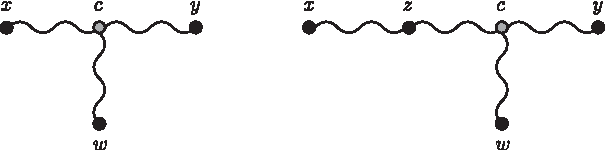
Case i when w is not in (x, y)-path but it is connected to it by a node c and the new z is in (c, y)-path.

From the tree d_wx + d_wy − d_xy = 2d_cw = d_wz + d_wy − d_zy, so d_wz = d_wx − d_xy + d_zy.

The four-point condition for these points can be verified by the labeling that results in M_xw + M_zy = M_xy + M_zw. Thus, M_wx − M_xy = M_zw − M_zy. Then \documentclass{aastex}\usepackage{amsbsy}\usepackage{amsfonts}\usepackage{amssymb}\usepackage{bm}\usepackage{mathrsfs}\usepackage{pifont}\usepackage{stmaryrd}\usepackage{textcomp}\usepackage{portland, xspace}\usepackage{amsmath, amsxtra}\pagestyle{empty}\DeclareMathSizes{10}{9}{7}{6}\begin{document} \begin{align*}d_{zw} & = d_{wx} - d_{xy} + d_{zy} \\ & = M_{wx} - M_{xy} + d_{zy} \quad ({\rm induction \ hypothesis}) \\ & = M_{zw} - M_{zy} + d_{zy} \quad ({\rm rewriting} \ M_{wx} - M_{xy}) \\ & = M_{zw} - M_{zy} + M_{zy} \quad ({\rm construction}) \\ & = M_{zw}\end{align*} \end{document}

Note that this proof works also for the case in which c = w.

Finally, let us see what happens when there is already an internal node c in the position where z should be added. Node c is a hypothetical ancestor, otherwise z would be already in the tree. It is enough to transform this internal node c into the live ancestral z = o_k+1. We only need to show that d_zw = M_zw, for any live node w connected to z without using edges or nodes in (x, y)-path, because the situations in which there are nodes from (x, y)-path are covered above. (Fig. 6).

OPEN IN VIEWER

FIG. 6.

Case i when a hypothetical c exists at z's position, and c is replaced by z.

The four-point condition for these points can be verified by the labeling that results in M_zw + M_yx = M_xz + M_wy. Then, \documentclass{aastex}\usepackage{amsbsy}\usepackage{amsfonts}\usepackage{amssymb}\usepackage{bm}\usepackage{mathrsfs}\usepackage{pifont}\usepackage{stmaryrd}\usepackage{textcomp}\usepackage{portland, xspace}\usepackage{amsmath, amsxtra}\pagestyle{empty}\DeclareMathSizes{10}{9}{7}{6}\begin{document} \begin{align*}2d_{zw} & = d_{xw} + d_{yw} - d_{xy} \qquad \qquad \qquad \quad ({\rm from} \ T^{k + 1}) \\ 2d_{zw} & = d_{xw} + d_{yw} - M_{xy} \qquad \qquad \qquad \quad ({\rm induction \ hypothesis}) \\ 2d_{zw} & = d_{xw} + d_{yw} - M_{xz} - M_{wy} + M_{zw} \quad ({\rm rewriting} \ M_{xy}) \\ 2d_{zw} & = d_{xw} + M_{yw} - M_{xz} - M_{wy} + M_{zw} \quad \quad ({\rm induction \ hypothesis}) \\ 2d_{zw} & = d_{xw} - d_{xz} + M_{zw} \qquad \qquad \qquad ({\rm construction}) \\ 2d_{zw} & = d_{zw} + M_{zw} \qquad \qquad \qquad \qquad ({\rm from} \ T^{k + 1}) \\ d_{zw} & = M_{zw}\end{align*} \end{document}

This concludes Case i.

Case ii: M_xz = M_xy + M_yz. This case is similar to Case 2 of the basis, in the sense that z is added to T by connecting it to y through a new edge (y, z).

We need to show that, d_zw = M_zw, for any node w in T^k+1, w ≠ x, y. Let w ≠ x, y be a node of T^k+1 and c the node connecting w to the path that connects x to y. (Fig. 7).

OPEN IN VIEWER

FIG. 7.

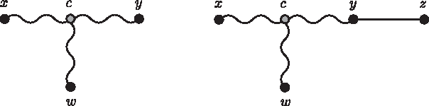
In Case ii, the new node z is connected to y by a new edge.

The four-point condition for these points can be verified by the labeling that results in M_xy + M_wz = M_xz + M_yw. Then, \documentclass{aastex}\usepackage{amsbsy}\usepackage{amsfonts}\usepackage{amssymb}\usepackage{bm}\usepackage{mathrsfs}\usepackage{pifont}\usepackage{stmaryrd}\usepackage{textcomp}\usepackage{portland, xspace}\usepackage{amsmath, amsxtra}\pagestyle{empty}\DeclareMathSizes{10}{9}{7}{6}\begin{document} \begin{align*}d_{zw} & = d_{wy} + d_{yz} \qquad \qquad \qquad ({\rm from \ the \ tree}) \\ & = M_{wy} + d_{yz} \qquad \qquad \quad\;\; ({\rm induction \ hypothesis}) \\ & = M_{xy} + M_{wz} - M_{xz} - d_{yz} \quad ({\rm rewriting} \ M_{yw}) \quad \\ & = d_{xy} + M_{wz} - d_{xz} + d_{yz} \quad\;\; ({\rm induction \ hypothesis}) \\ & = M_{wz}\end{align*} \end{document}

Notice that this proof holds also in the case where w = c.

Case iii: M_yz = M_xy + M_xz. This case is similar to Case 3 of the basis, and node z is added on the same way. The proof is analogous to the one given in Case ii.

If none of the cases i, ii, and iii happens, then we try to add the new node z to T^k through an edge connecting z and a node c in the (x, y)-path, as we do in Case 4 of the basis. There are three possibilities to consider.

Case iv-a: There is no node c in T^k as it also happens in Case 4 of the basis. We create this new node c as a hypothetical ancestor and connect c to z through a new edge (c, z) with length (M(z, x) + M(z, y) − M(x, y))/2.

We need to show that d_wz = M_wz for every w ≠ x, y. Let us suppose that there is a path from v to w, where v is a node in the (x, c)-path. The case where v is in the (c, y)-path is analogous (Fig. 8).

OPEN IN VIEWER

FIG. 8.

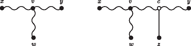
In Case iv-a, the new node z is connected to a new hypothetical ancestor c by an edge.

The four-point condition for these points can be verified by the labeling that results in M_xy + M_wz = M_xz + M_yw. From the tree, d_zw + d_zy − d_wy = 2d_cz = d_xz + d_zy − d_xy. So d_zw = d_xz − d_xy + d_wy. \documentclass{aastex}\usepackage{amsbsy}\usepackage{amsfonts}\usepackage{amssymb}\usepackage{bm}\usepackage{mathrsfs}\usepackage{pifont}\usepackage{stmaryrd}\usepackage{textcomp}\usepackage{portland, xspace}\usepackage{amsmath, amsxtra}\pagestyle{empty}\DeclareMathSizes{10}{9}{7}{6}\begin{document} \begin{align*}d_{zw} & = d_{xz} - d_{xy} + d_{wy} \\ & = d_{xz} - M_{xy} + M_{wy} \quad\;\; \ ({\rm induction}) \\ & = d_{xz} + M_{wz} - M_{xz} \qquad ({\rm rewriting} \ M_{wy} - M_{xy}) \\ & = M_{xz} + M_{wz} - M_{xz} \qquad ({\rm construction}) \\ & = M_{wz}\end{align*} \end{document}

Note that this proof works also for the case in which v = w.

Case iv-b: Suppose that there is already a node c in T^k, as in Case 4 of the basis, such that c has degree 2. Because we only create a hypothetical node with degree 3, c is a live ancestor. In this case, we just add z to T^k and connect z to c through a new edge (z, c) with the same length as in Case iv-a. The proof that d_wz = M_wz for every w ≠ x, y is similar to that provided for Case iv-a.

Case iv-c: Now, consider the case in which there is a node c in T^k, as in Case 4 of the basis, but c has degree >2. This means that there is at least another leaf w connected to c through a path not using any vertex or edge in (x, y)-path. To solve this case, find any pair of leaves r, s such that c is in (r, s)-path and one of the previous cases i, ii, iii, iv-a, and iv-b holds, and apply the appropriated case. If there is no such pair of leaves r, s, then just add z to the tree and connect it to c through a new edge (c, z).

We need to show that d_wz = M_wz for every w ≠ x, y. If w is either in the (x, y)-path, or there is a path from d to w, where d is a node in the (x, c)-path, then the proofs are similar to the previous ones. Otherwise w is in a path connected to c, as shown in Figure 9.

OPEN IN VIEWER

FIG. 9.

In Case iv-c, the new node z is connected to an existing hypothetical ancestor c by an edge.

The four-point condition for these points can be verified by the labeling that results in M_xy + M_wz = M_xz + M_yw. From the tree, d_xz + d_zy − d_xy = 2d_cz = d_zw + d_zy − d_wy, and the proof follows exactly as the one for Case iv-a. ▪

The constructive proof of Theorem 1 gives us an algorithm to build the live phylogeny given an additive matrix. The algorithm consists of starting with two objects connected by an edge and applying, in each step, one of the described cases. This algorithm clearly has polynomial time in the number of objects, since the test for the correct case can be done in constant time, except for Case iv-b, where we need to find a pair of leaves satisfying any of the other cases. Because there are O(k²) possible pairs of leaves, in each step k, the total time is O(n³).

3. Character States Live Phylogeny

For this problem, one is interested in building a phylogenetic rooted tree that explains the evolutionary relationship among objects, based on states of characters that each object possesses. More formally, the input is an n × m matrix M, where M_i,j is the state of character j for object i.

In the related literature, the character-based phylogeny problem has been approached, considering the number of possible states for each character and whether or not there is an order relation defined for character states. If the number of states is fixed, then the problem can be easily solved. Otherwise, it is NP-hard. When the order is totally defined, then there is a polynomial-time algorithm for the problem. Otherwise, the problem is also NP-hard (Setubal and Meidanis, 1997).

Another issue concerns more complicated evolutionary facts, such as reversal and parallel evolution events. A reversal happens when a character changes back to a previous state. A parallel evolution happens when a character changes to the same state in two distinct lineages. When there are no such events, the problem is known as the perfect phylogeny problem. Other works in the literature concern minimizing the number of reversals and parallel evolution events to obtain a perfect phylogeny or maximizing the number of characters that admit a perfect phylogeny (Setubal and Meidanis, 1997).

In this work, we introduce the perfect live phylogeny with two character states. Let M be an n × m binary matrix whose rows are labeled \documentclass{aastex}\usepackage{amsbsy}\usepackage{amsfonts}\usepackage{amssymb}\usepackage{bm}\usepackage{mathrsfs}\usepackage{pifont}\usepackage{stmaryrd}\usepackage{textcomp}\usepackage{portland, xspace}\usepackage{amsmath, amsxtra}\pagestyle{empty}\DeclareMathSizes{10}{9}{7}{6}\begin{document} $$o_1 , o_2 \ldots o_n$$ \end{document} , whose columns are labeled \documentclass{aastex}\usepackage{amsbsy}\usepackage{amsfonts}\usepackage{amssymb}\usepackage{bm}\usepackage{mathrsfs}\usepackage{pifont}\usepackage{stmaryrd}\usepackage{textcomp}\usepackage{portland, xspace}\usepackage{amsmath, amsxtra}\pagestyle{empty}\DeclareMathSizes{10}{9}{7}{6}\begin{document} $$c_1 , c_2 \ldots c_m$$ \end{document} , and whose columns are pairwise disjoint or comparable. A live perfect phylogeny for M is a rooted tree T such that:

1. Each edge in T is labeled with a distinct c_j;

Observe that this definition allows T to have labeled internal nodes. Then, objects given in the input may be ancestors in the phylogeny.

The polynomial time algorithm to solve this problem is presented in Figure 10. It is a simple adaptation of the algorithm for perfect phylogeny by Waterman et al. (1977). The input is a binary matrix M with columns sorted in nonincreasing order of the number of 1s. An example input and tree appear in Figure 11.

OPEN IN VIEWER

FIG. 10.

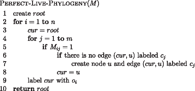
Perfect live phylogeny polynomial-time algorithm.

OPEN IN VIEWER

FIG. 11.

A binary matrix with columns sorted in nonincreasing order of the number of 1s, and the corresponding live phylogeny tree, in which B is a live ancestor.

For the correctness of the algorithm, let T be the tree whose root is returned by the algorithm. It is easy to see that each o_i is used to label exactly one node of T. It is also easy to see that no edge is created without a label. Now, suppose that two edges in T were labeled c_j, while processing objects o_i and o_k, i < k. The ordering of the columns of M, and the fact that each pair of columns of M is either comparable or disjoint, guarantee that M_i,j′ = M_k,j′, 1 ≤ j′ ≤ j − 1. Thus, by construction, the paths between the root and both edges labeled c_j must be the same, which is a contradiction.

To see that if M_i,j = 1 then c_j is in the path from the root of T to the node labeled o_i, it is enough to see that during the processing of row i of M, either the edge c_j is created or traversed. By the other side, if edge c_j is in the path between the root and the node labeled o_i, then o_i was labeled after creating or the traversing of edge c_j, and that happens only if M_i,j = 1.

4. Conclusions

Live phylogeny generalizes phylogeny while broadening its application to other areas distinct from molecular biology, such as visualization, data mining, and forensics. As with phylogeny, live phylogeny will certainly lead to NP-hard problems when the restrictions we considered here are released, namely the absence of reversals and parallel evolution, and additivity. A broad class of approximation algorithms and heuristics may then be explored for the problem. We conclude our article noting that applications beyond molecular biology deal with very large datasets, and large-scale techniques may be considered as well.