Recovering the Treelike Trend of Evolution Despite Extensive Lateral Genetic Transfer: A Probabilistic Analysis

Abstract

Lateral gene transfer (LGT) is a common mechanism of nonvertical evolution, during which genetic material is transferred between two more or less distantly related organisms. It is particularly common in bacteria where it contributes to adaptive evolution with important medical implications. In evolutionary studies, LGT has been shown to create widespread discordance between gene trees as genomes become mosaics of gene histories. In particular, the Tree of Life has been questioned as an appropriate representation of bacterial evolutionary history. Nevertheless a common hypothesis is that prokaryotic evolution is primarily treelike, but that the underlying trend is obscured by LGT. Extensive empirical work has sought to extract a common treelike signal from conflicting gene trees. Here we give a probabilistic perspective on the problem of recovering the treelike trend despite LGT. Under a model of randomly distributed LGT, we show that the species phylogeny can be reconstructed even in the presence of surprisingly many (almost linear number of) LGT events per gene tree. Our results, which are optimal up to logarithmic factors, are based on the analysis of a robust, computationally efficient reconstruction method and provides insight into the design of such methods. Finally, we show that our results have implications for the discovery of highways of gene sharing.

1. Introduction

High-throughput sequencing is transforming the study of evolution by allowing the integration of genome analysis and systematic studies, an area called phylogenomics (Eisen and Fraser, 2003; Delsuc et al., 2005). An important step in most phylogenomic analyses is the reconstruction of a tree of ancestor-descendant relationships—a gene tree—for each family of orthologous genes in a dataset. Such analyses have revealed widespread discordance among gene trees (Galtier and Daubin, 2008), leading some to question the meaningfulness of the Tree of Life (Gogarten et al., 2002; Zhaxybayeva et al., 2004; Gogarten and Townsend, 2005; Bapteste et al., 2005; Doolittle and Bapteste, 2007; Koonin, 2007). In addition to statistical errors in gene tree estimation, various mechanisms commonly lead to incongruences between inferred gene histories, including hybridization events, duplications and losses in gene families, incomplete lineage sorting, and lateral genetic transfers (Maddison, 1997).

Here we study specifically lateral gene transfer (LGT), that is, the nonvertical transfer of genes between more or less distantly related organisms (as opposed to the standard vertical transmission between parent and offspring). Estimates of the fraction of genes that have undergone LGT vary widely—with some as high as 99% (see, e.g., Dagan and Martin, 2006; Galtier and Daubin, 2008; and references therein). LGT is particularly common in bacterial evolution and it has been recognized to play an important role in microbial adaptation, selection, and evolution, with implications in the study of infectious diseases (Smets and Barkay, 2005). As a result, the bacterial phylogeny is usually inferred from genes that are thought to be immune to LGT, typically ribosomal RNA genes. However, there is growing evidence that even such genes have in fact experienced LGT (Yap et al., 1999; van Berkum et al., 2003; Schouls et al., 2003; Dewhirst et al., 2005). In any case, LGT appears to be a major source of conflict between gene trees that must be taken into account appropriately in phylogenomic analyses, in particular when building phylogenies. This is the problem we address in this article.

Despite the confounding effect of LGT, we operate under the prevailing assumption that the evolution of organisms is governed primarily by vertical inheritance. In particular, we ask the following:

1. How much genetic transfer can be handled before the treelike signal is completely erased?

2. What phylogenetic reconstruction methods are most effective under this hypothesis?

These questions, and other related issues, have been the subject of some empirical and simulation-based work (Beiko et al., 2005; Ge et al., 2005; Galtier, 2007; Puigbo et al., 2009, 2010; Koonin et al., 2011). See also Galtier and Daubin (2008) and Ragan and Beiko (2009) for enlightening discussions. In particular, there is ample evidence that a strong treelike signal can be extracted in the presence of extensive LGT [although some debate remains on this question (Gogarten et al., 2002)].

In this article, we provide the first (to our knowledge) mathematical analysis of the issues above. We work under a stochastic model of gene-tree topologies positing that LGT events occur at more or less random locations on the species phylogeny (Galtier, 2007). In our main result, we establish quantitative bounds implying that surprisingly high levels of LGT—almost linear in the number of branches for each gene—can be handled by simple, computationally efficient inference procedures. That amount of genetic transfer appears to be much higher than known empirical estimates of LGT frequency based on genomic datasets in prokaryotes.¹ Hence, our results indicate that an accurate, reliable bacterial phylogeny should be reconstructible if the vertical inheritance hypothesis is correct. We prove that our bound on the achievable rate of LGT is tight up to logarithmic factors. We also show that constraining LGT to closely related species makes the tree reconstruction problem significantly easier.

Our theoretical approach complements simulation-based studies by allowing a broad range of parameters and tree shapes to be considered. Moreover, our analysis provides new insights into the design of effective reconstruction methods in the presence of LGT. More precisely, we focus on methodologies—both distance-based (Kim and Salisbury, 2001) and quartet-based (Zhaxybayeva et al., 2006)—that derive their statistical power from the aggregation of basic topological information across genes.

In addition, we study the effect of so-called highways of gene sharing; roughly, preferred genetic exchanges between specific groups of species. Beiko et al. (2005) provided empirical evidence for the existence of such highways. To identify highways, they inferred LGT events by reconciling gene trees with a trusted species tree. In subsequent work, Bansal et al. (2011) formalized the problem and designed a fast highway detection algorithm that aggregates conflicting signal across genes rather than solving the difficult LGT inference problem on each gene tree. Similarly to Beiko et al. (2005), Bansal et al. (2011) rely on a trusted species tree.

Here we show that a species phylogeny can be reliably estimated in the presence of both random LGT events and highways of LGT, as long as such highways involve a small enough fraction of genes. Under extra assumptions, we also design an algorithm for inferring the location of highways. Because we first recover the species phylogeny, our highway reconstruction algorithm does not require a trusted species tree. In essence, our results on highways indicate that robust phylogeny reconstruction in the presence of random LGT extends to a phylogenetic network setting. For background on phylogenetic networks, see, for example, Huson et al. (2010).

We note that there exist related lines of work in phylogenomics, addressing the issue of incomplete lineage sorting (Degnan and Rosenberg, 2009) in the presence of gene transfers and hybridization events (Than et al., 2007; Joly et al., 2009; Kubatko, 2009; Meng and Kubatko, 2009; Chung and Ane, 2011; Yu et al., 2011) as well as work on probabilistic models involving gene duplications and losses (Arvestad et al., 2009; Csürös and Miklós, 2006).

The rest of the article is organized as follows. In Section 2, we define a stochastic model of LGT and state our main results. A high-level description of our analysis is given in Section 3. Finally, in Section 4, we extend our results to highways of gene sharing. [The results presented here were announced without proof in Roch and Snir (2012).]

2. Model and Main Results

Before stating our main results, we present a stochastic model of LGT. Roughly, following Galtier (2007), we assume that LGT events occur more or less at random along the species phylogeny. Such a model appears to be consistent with empirical evidence (Galtier and Daubin, 2008).

Notation Recall that, for functions f (n), g(n), f=O(g) means that there is constant C > 0 such that f (n) ≤ Cg(n) for all n large enough. Similarly, f=Ω(g) indicates f (n) ≥ C′g(n) for C′ > 0. In addition f=Θ(g) is equivalent to f=O(g) and f=Ω(g). By polynomial in n, we mean \documentclass{aastex}\usepackage{amsbsy}\usepackage{amsfonts}\usepackage{amssymb}\usepackage{bm}\usepackage{mathrsfs}\usepackage{pifont}\usepackage{stmaryrd}\usepackage{textcomp}\usepackage{portland, xspace}\usepackage{amsmath, amsxtra}\pagestyle{empty}\DeclareMathSizes{10}{9}{7}{6}\begin{document} $$O ( n^{C^{ \prime \prime}} )$$ \end{document} for some constant C″ > 0. We use the notation \documentclass{aastex}\usepackage{amsbsy}\usepackage{amsfonts}\usepackage{amssymb}\usepackage{bm}\usepackage{mathrsfs}\usepackage{pifont}\usepackage{stmaryrd}\usepackage{textcomp}\usepackage{portland, xspace}\usepackage{amsmath, amsxtra}\pagestyle{empty}\DeclareMathSizes{10}{9}{7}{6}\begin{document} $${\mathbb P} [ { \cal E} _0 \mid { \cal E}_1 ]$$ \end{document} for the conditional probability of \documentclass{aastex}\usepackage{amsbsy}\usepackage{amsfonts}\usepackage{amssymb}\usepackage{bm}\usepackage{mathrsfs}\usepackage{pifont}\usepackage{stmaryrd}\usepackage{textcomp}\usepackage{portland, xspace}\usepackage{amsmath, amsxtra}\pagestyle{empty}\DeclareMathSizes{10}{9}{7}{6}\begin{document} $${ \cal E}_0$$ \end{document} given \documentclass{aastex}\usepackage{amsbsy}\usepackage{amsfonts}\usepackage{amssymb}\usepackage{bm}\usepackage{mathrsfs}\usepackage{pifont}\usepackage{stmaryrd}\usepackage{textcomp}\usepackage{portland, xspace}\usepackage{amsmath, amsxtra}\pagestyle{empty}\DeclareMathSizes{10}{9}{7}{6}\begin{document} $${ \cal E}{ \cal }_1$$ \end{document} .

2.1. Stochastic model of LGT

Gene trees and species phylogeny

A species phylogeny (or phylogeny for short) is a graphical representation of the speciation history of a group of organisms. The leaves correspond to extant or extinct species. Each branching indicates a speciation event. Moreover, we associate to each edge a positive value corresponding to the time elapsed along that edge. For a tree \documentclass{aastex}\usepackage{amsbsy}\usepackage{amsfonts}\usepackage{amssymb}\usepackage{bm}\usepackage{mathrsfs}\usepackage{pifont}\usepackage{stmaryrd}\usepackage{textcomp}\usepackage{portland, xspace}\usepackage{amsmath, amsxtra}\pagestyle{empty}\DeclareMathSizes{10}{9}{7}{6}\begin{document} $${ \cal T} = ( \nu , { \cal E} )$$ \end{document} with leaf set L and a subset of leaves X ⊆ L, we let \documentclass{aastex}\usepackage{amsbsy}\usepackage{amsfonts}\usepackage{amssymb}\usepackage{bm}\usepackage{mathrsfs}\usepackage{pifont}\usepackage{stmaryrd}\usepackage{textcomp}\usepackage{portland, xspace}\usepackage{amsmath, amsxtra}\pagestyle{empty}\DeclareMathSizes{10}{9}{7}{6}\begin{document} $${ \cal T} \mid X$$ \end{document} be the restriction of \documentclass{aastex}\usepackage{amsbsy}\usepackage{amsfonts}\usepackage{amssymb}\usepackage{bm}\usepackage{mathrsfs}\usepackage{pifont}\usepackage{stmaryrd}\usepackage{textcomp}\usepackage{portland, xspace}\usepackage{amsmath, amsxtra}\pagestyle{empty}\DeclareMathSizes{10}{9}{7}{6}\begin{document} $${ \cal T}$$ \end{document} to X, that is, the subtree of \documentclass{aastex}\usepackage{amsbsy}\usepackage{amsfonts}\usepackage{amssymb}\usepackage{bm}\usepackage{mathrsfs}\usepackage{pifont}\usepackage{stmaryrd}\usepackage{textcomp}\usepackage{portland, xspace}\usepackage{amsmath, amsxtra}\pagestyle{empty}\DeclareMathSizes{10}{9}{7}{6}\begin{document} $${ \cal T}$$ \end{document} where we keep only those vertices and edges on paths connecting two leaves in X. We say that \documentclass{aastex}\usepackage{amsbsy}\usepackage{amsfonts}\usepackage{amssymb}\usepackage{bm}\usepackage{mathrsfs}\usepackage{pifont}\usepackage{stmaryrd}\usepackage{textcomp}\usepackage{portland, xspace}\usepackage{amsmath, amsxtra}\pagestyle{empty}\DeclareMathSizes{10}{9}{7}{6}\begin{document} $${ \cal T}$$ \end{document} agrees (or is consistent) with \documentclass{aastex}\usepackage{amsbsy}\usepackage{amsfonts}\usepackage{amssymb}\usepackage{bm}\usepackage{mathrsfs}\usepackage{pifont}\usepackage{stmaryrd}\usepackage{textcomp}\usepackage{portland, xspace}\usepackage{amsmath, amsxtra}\pagestyle{empty}\DeclareMathSizes{10}{9}{7}{6}\begin{document} $${ \cal T} \mid X$$ \end{document} .

Definition 1 (Phylogeny)

A (species) phylogeny T_s=(V_s, E_s, L_s; r, τ) is a rooted tree with vertex set V_s, edge set E_s and n (labeled) leaves \documentclass{aastex}\usepackage{amsbsy}\usepackage{amsfonts}\usepackage{amssymb}\usepackage{bm}\usepackage{mathrsfs}\usepackage{pifont}\usepackage{stmaryrd}\usepackage{textcomp}\usepackage{portland, xspace}\usepackage{amsmath, amsxtra}\pagestyle{empty}\DeclareMathSizes{10}{9}{7}{6}\begin{document} $$L_s = [ n ] = \{ 1 , \ldots , n \} $$ \end{document} such that 1) the degree of all internal vertices V_s − L_s is exactly 3 except the root r, which has degree 2; and 2) the edges are assigned interspeciation times τ : E_s → (0, +∞). We assume that T_s includes n⁺ > 0 extant species \documentclass{aastex}\usepackage{amsbsy}\usepackage{amsfonts}\usepackage{amssymb}\usepackage{bm}\usepackage{mathrsfs}\usepackage{pifont}\usepackage{stmaryrd}\usepackage{textcomp}\usepackage{portland, xspace}\usepackage{amsmath, amsxtra}\pagestyle{empty}\DeclareMathSizes{10}{9}{7}{6}\begin{document} $$L_s^{+}$$ \end{document} and n⁻ ≥ 0 extinct species \documentclass{aastex}\usepackage{amsbsy}\usepackage{amsfonts}\usepackage{amssymb}\usepackage{bm}\usepackage{mathrsfs}\usepackage{pifont}\usepackage{stmaryrd}\usepackage{textcomp}\usepackage{portland, xspace}\usepackage{amsmath, amsxtra}\pagestyle{empty}\DeclareMathSizes{10}{9}{7}{6}\begin{document} $$L_s^{ -}$$ \end{document} , where n=n⁺ + n⁻. We also associate to each edge \documentclass{aastex}\usepackage{amsbsy}\usepackage{amsfonts}\usepackage{amssymb}\usepackage{bm}\usepackage{mathrsfs}\usepackage{pifont}\usepackage{stmaryrd}\usepackage{textcomp}\usepackage{portland, xspace}\usepackage{amsmath, amsxtra}\pagestyle{empty}\DeclareMathSizes{10}{9}{7}{6}\begin{document} $$e \in E_s$$ \end{document} in T_s a rate of lateral gene transfer 0 < λ(e) < +∞. We denote by \documentclass{aastex}\usepackage{amsbsy}\usepackage{amsfonts}\usepackage{amssymb}\usepackage{bm}\usepackage{mathrsfs}\usepackage{pifont}\usepackage{stmaryrd}\usepackage{textcomp}\usepackage{portland, xspace}\usepackage{amsmath, amsxtra}\pagestyle{empty}\DeclareMathSizes{10}{9}{7}{6}\begin{document} $$T_s^ {+} = ( V_s^ {+} , E_s^ {+} , L_s^ {+} ;r , \tau^ {+} )$$ \end{document} , the subtree of T_s restricted to the extant leaves \documentclass{aastex}\usepackage{amsbsy}\usepackage{amsfonts}\usepackage{amssymb}\usepackage{bm}\usepackage{mathrsfs}\usepackage{pifont}\usepackage{stmaryrd}\usepackage{textcomp}\usepackage{portland, xspace}\usepackage{amsmath, amsxtra}\pagestyle{empty}\DeclareMathSizes{10}{9}{7}{6}\begin{document} $$L_s^ {+}$$ \end{document} , that is, \documentclass{aastex}\usepackage{amsbsy}\usepackage{amsfonts}\usepackage{amssymb}\usepackage{bm}\usepackage{mathrsfs}\usepackage{pifont}\usepackage{stmaryrd}\usepackage{textcomp}\usepackage{portland, xspace}\usepackage{amsmath, amsxtra}\pagestyle{empty}\DeclareMathSizes{10}{9}{7}{6}\begin{document} $$T_s^ {+} = T_s \mid L_s^ {+}$$ \end{document} rooted at the most recent common ancestor of \documentclass{aastex}\usepackage{amsbsy}\usepackage{amsfonts}\usepackage{amssymb}\usepackage{bm}\usepackage{mathrsfs}\usepackage{pifont}\usepackage{stmaryrd}\usepackage{textcomp}\usepackage{portland, xspace}\usepackage{amsmath, amsxtra}\pagestyle{empty}\DeclareMathSizes{10}{9}{7}{6}\begin{document} $$L_s^ {+}$$ \end{document} . We further suppress vertices of degree 2 in \documentclass{aastex}\usepackage{amsbsy}\usepackage{amsfonts}\usepackage{amssymb}\usepackage{bm}\usepackage{mathrsfs}\usepackage{pifont}\usepackage{stmaryrd}\usepackage{textcomp}\usepackage{portland, xspace}\usepackage{amsmath, amsxtra}\pagestyle{empty}\DeclareMathSizes{10}{9}{7}{6}\begin{document} $$T_s^ {+}$$ \end{document} except the root (in which case we add up the branch lengths to obtain τ⁺). We call \documentclass{aastex}\usepackage{amsbsy}\usepackage{amsfonts}\usepackage{amssymb}\usepackage{bm}\usepackage{mathrsfs}\usepackage{pifont}\usepackage{stmaryrd}\usepackage{textcomp}\usepackage{portland, xspace}\usepackage{amsmath, amsxtra}\pagestyle{empty}\DeclareMathSizes{10}{9}{7}{6}\begin{document} $$T_s^ {+}$$ \end{document} the extant phylogeny. We assume that \documentclass{aastex}\usepackage{amsbsy}\usepackage{amsfonts}\usepackage{amssymb}\usepackage{bm}\usepackage{mathrsfs}\usepackage{pifont}\usepackage{stmaryrd}\usepackage{textcomp}\usepackage{portland, xspace}\usepackage{amsmath, amsxtra}\pagestyle{empty}\DeclareMathSizes{10}{9}{7}{6}\begin{document} $$T_s^ {+}$$ \end{document} is ultrametric, that is, from every node, the path lengths from that node to all its descendant leaves are equal.

Although we are ultimately interested in recovering the extant phylogeny, we include extinct species in the model as they can be involved in LGT events that affect the extant restriction of the tree (see, for example, Maddison, 1997).

To infer the species phylogeny, we first reconstruct gene trees, that is, trees of ancestor-descendant relationships for orthologous genes or loci. Phylogenomic studies have revealed extensive discordance between such gene trees (e.g., Bapteste et al., 2005; Doolittle and Bapteste, 2007).

Definition 2 (Gene tree)

A gene tree T_g=(V_g, E_g, L_g; ω_g) for gene g is an unrooted tree with vertex set V_g, edge set E_g and 0 < n_g ≤ n (labeled) leaves \documentclass{aastex}\usepackage{amsbsy}\usepackage{amsfonts}\usepackage{amssymb}\usepackage{bm}\usepackage{mathrsfs}\usepackage{pifont}\usepackage{stmaryrd}\usepackage{textcomp}\usepackage{portland, xspace}\usepackage{amsmath, amsxtra}\pagestyle{empty}\DeclareMathSizes{10}{9}{7}{6}\begin{document} $$L_g \subseteq \{ 1 , \ldots , n \} $$ \end{document} with ∣L_g∣=n_g such that 1) the degree of every internal vertex is either 2 or 3, and 2) the edges are assigned branch lengths ω_g : E_g → (0, +∞). We let \documentclass{aastex}\usepackage{amsbsy}\usepackage{amsfonts}\usepackage{amssymb}\usepackage{bm}\usepackage{mathrsfs}\usepackage{pifont}\usepackage{stmaryrd}\usepackage{textcomp}\usepackage{portland, xspace}\usepackage{amsmath, amsxtra}\pagestyle{empty}\DeclareMathSizes{10}{9}{7}{6}\begin{document} $${ \cal T}_g = { \cal T} [ T_g ]$$ \end{document} be the topology of T_g where each internal vertex of degree 2 is suppressed.

Remark 1 (Gene trees vs. species phylogeny)

As we will discuss below, gene trees are derived from— or “evolve” on—the species phlyogeny. They may differ from the species phylogeny for various reasons. First, in our model, their branch lengths represent expected numbers of substitutions, instead of time elapsed. Moreover, their topology may differ as a result, in our case, of LGT events. See more details below.

Remark 2 (Rooted vs. unrooted)

Our stochastic model of LGT requires a rooted species phylogeny as time plays an important role in constraining valid LGT events (see, e.g., Jin et al., 2009). In particular, our results rely on the ultrametricity property of the extant phylogeny. In contrast, branch lengths in gene trees correspond to expected numbers of substitutions. As a result, gene trees are typically unrooted and do not satisfy ultrametricity.

Remark 3 (Taxon sampling)

Each leaf in a gene tree corresponds to an extant species in the species phylogeny. However, because of gene loss and taxon sampling, a taxon may not be represented in every gene tree.

Remark 4 (Branch lengths)

Each branch e in a gene tree T_g corresponds to a full or partial edge in the species phylogeny T_s. In particular, we allow internal vertices of degree 2 in a gene tree to potentially delineate between two consecutive species edges. We allow the branch lengths ω_g(e) to be arbitrary, but one could easily consider cases where the branch lengths are determined by interspeciation times, lineage-specific rates of substitution, and gene-specific rates of substitution. The branch lengths will play a role in Section 5.

Random LGT

We formalize a stochastic model of LGT similar to Galtier's (Galtier, 2007). See also Kim and Salisbury (2001); Suchard (2005); and Jin et al. (2006) for related models. The model accounts for LGT events originating at random locations on the species phylogeny with LGT rate λ(e) prevailing along edge e.

We will need the following notation. Let T_s=(V_s, E_s, L_s; r, τ) be a fixed species phylogeny. By a location in T_s, we mean any position along T_s seen as a continuous object (also called \documentclass{aastex}\usepackage{amsbsy}\usepackage{amsfonts}\usepackage{amssymb}\usepackage{bm}\usepackage{mathrsfs}\usepackage{pifont}\usepackage{stmaryrd}\usepackage{textcomp}\usepackage{portland, xspace}\usepackage{amsmath, amsxtra}\pagestyle{empty}\DeclareMathSizes{10}{9}{7}{6}\begin{document} $${\mathbb R}$$ \end{document} -tree), that is, a point x along an edge \documentclass{aastex}\usepackage{amsbsy}\usepackage{amsfonts}\usepackage{amssymb}\usepackage{bm}\usepackage{mathrsfs}\usepackage{pifont}\usepackage{stmaryrd}\usepackage{textcomp}\usepackage{portland, xspace}\usepackage{amsmath, amsxtra}\pagestyle{empty}\DeclareMathSizes{10}{9}{7}{6}\begin{document} $$e \in E_s$$ \end{document} . We write \documentclass{aastex}\usepackage{amsbsy}\usepackage{amsfonts}\usepackage{amssymb}\usepackage{bm}\usepackage{mathrsfs}\usepackage{pifont}\usepackage{stmaryrd}\usepackage{textcomp}\usepackage{portland, xspace}\usepackage{amsmath, amsxtra}\pagestyle{empty}\DeclareMathSizes{10}{9}{7}{6}\begin{document} $$x \in e$$ \end{document} in that case. We denote the set of locations in T_s by \documentclass{aastex}\usepackage{amsbsy}\usepackage{amsfonts}\usepackage{amssymb}\usepackage{bm}\usepackage{mathrsfs}\usepackage{pifont}\usepackage{stmaryrd}\usepackage{textcomp}\usepackage{portland, xspace}\usepackage{amsmath, amsxtra}\pagestyle{empty}\DeclareMathSizes{10}{9}{7}{6}\begin{document} $${ \cal X}_s$$ \end{document} . For any two locations x, y in \documentclass{aastex}\usepackage{amsbsy}\usepackage{amsfonts}\usepackage{amssymb}\usepackage{bm}\usepackage{mathrsfs}\usepackage{pifont}\usepackage{stmaryrd}\usepackage{textcomp}\usepackage{portland, xspace}\usepackage{amsmath, amsxtra}\pagestyle{empty}\DeclareMathSizes{10}{9}{7}{6}\begin{document} $${ \cal X}_s$$ \end{document} , we let MRCA(x, y) be their most recent common ancestor (MRCA) in T_s, and we let τ(x, y) be the length of the path connecting x and y in T_s under the metric naturally defined by the weights \documentclass{aastex}\usepackage{amsbsy}\usepackage{amsfonts}\usepackage{amssymb}\usepackage{bm}\usepackage{mathrsfs}\usepackage{pifont}\usepackage{stmaryrd}\usepackage{textcomp}\usepackage{portland, xspace}\usepackage{amsmath, amsxtra}\pagestyle{empty}\DeclareMathSizes{10}{9}{7}{6}\begin{document} $$\{ \tau ( e ) , e \in E_s \} $$ \end{document} , interpolated linearly to locations along an edge. In words τ(x, y), which we refer to as the τ-distance between x and y, is the sum of times to x and y from MRCA(x, y). We say that two locations x, y are contemporaneous if their respective τ-distance to the root r is identical, that is, \documentclass{aastex}\usepackage{amsbsy}\usepackage{amsfonts}\usepackage{amssymb}\usepackage{bm}\usepackage{mathrsfs}\usepackage{pifont}\usepackage{stmaryrd}\usepackage{textcomp}\usepackage{portland, xspace}\usepackage{amsmath, amsxtra}\pagestyle{empty}\DeclareMathSizes{10}{9}{7}{6}\begin{document} \begin{align*}\tau ( x , r ) = \tau ( y , r ) .\end{align*} \end{document}

For R > 0, we let \documentclass{aastex}\usepackage{amsbsy}\usepackage{amsfonts}\usepackage{amssymb}\usepackage{bm}\usepackage{mathrsfs}\usepackage{pifont}\usepackage{stmaryrd}\usepackage{textcomp}\usepackage{portland, xspace}\usepackage{amsmath, amsxtra}\pagestyle{empty}\DeclareMathSizes{10}{9}{7}{6}\begin{document} \begin{align*}{ \cal C}_x^{ ( R ) } = \{ y \in { \cal X}_s : \tau ( r , x ) = \tau ( r , y ) , \ \tau ( x , y ) \leq 2 R \} \end{align*} \end{document}

be the set of locations contemporaneous to x at τ-distance at most 2R from x (or in other words, with MRCA at τ-distance at most R). In particular, \documentclass{aastex}\usepackage{amsbsy}\usepackage{amsfonts}\usepackage{amssymb}\usepackage{bm}\usepackage{mathrsfs}\usepackage{pifont}\usepackage{stmaryrd}\usepackage{textcomp}\usepackage{portland, xspace}\usepackage{amsmath, amsxtra}\pagestyle{empty}\DeclareMathSizes{10}{9}{7}{6}\begin{document} $${ \cal C}_x^{ ( \infty ) }$$ \end{document} denotes the set of all locations contemporaneous to x. We let \documentclass{aastex}\usepackage{amsbsy}\usepackage{amsfonts}\usepackage{amssymb}\usepackage{bm}\usepackage{mathrsfs}\usepackage{pifont}\usepackage{stmaryrd}\usepackage{textcomp}\usepackage{portland, xspace}\usepackage{amsmath, amsxtra}\pagestyle{empty}\DeclareMathSizes{10}{9}{7}{6}\begin{document} $$\Lambda ( e ) = \lambda ( e ) \tau ( e ) , e \in E_s$$ \end{document} . We note that, since λ(e) is the LGT rate on e, Λ(e) gives the expected number of LGT events along e. Further, we let \documentclass{aastex}\usepackage{amsbsy}\usepackage{amsfonts}\usepackage{amssymb}\usepackage{bm}\usepackage{mathrsfs}\usepackage{pifont}\usepackage{stmaryrd}\usepackage{textcomp}\usepackage{portland, xspace}\usepackage{amsmath, amsxtra}\pagestyle{empty}\DeclareMathSizes{10}{9}{7}{6}\begin{document} \begin{align*}\Lambda_{ \rm tot} = \sum_{e \in E_s} \Lambda ( e ) ,\end{align*} \end{document}

be the total LGT weight of the phylogeny and \documentclass{aastex}\usepackage{amsbsy}\usepackage{amsfonts}\usepackage{amssymb}\usepackage{bm}\usepackage{mathrsfs}\usepackage{pifont}\usepackage{stmaryrd}\usepackage{textcomp}\usepackage{portland, xspace}\usepackage{amsmath, amsxtra}\pagestyle{empty}\DeclareMathSizes{10}{9}{7}{6}\begin{document} \begin{align*}\Lambda = \sum_{e \in { \cal E} ( T_s \mid L_s^ {+} ) } \Lambda ( e ) ,\end{align*} \end{document}

be the total LGT weight of the extant phylogeny, where \documentclass{aastex}\usepackage{amsbsy}\usepackage{amsfonts}\usepackage{amssymb}\usepackage{bm}\usepackage{mathrsfs}\usepackage{pifont}\usepackage{stmaryrd}\usepackage{textcomp}\usepackage{portland, xspace}\usepackage{amsmath, amsxtra}\pagestyle{empty}\DeclareMathSizes{10}{9}{7}{6}\begin{document} $${ \cal E} ( T_s \mid L_s^ {+} )$$ \end{document} denotes the edge set of \documentclass{aastex}\usepackage{amsbsy}\usepackage{amsfonts}\usepackage{amssymb}\usepackage{bm}\usepackage{mathrsfs}\usepackage{pifont}\usepackage{stmaryrd}\usepackage{textcomp}\usepackage{portland, xspace}\usepackage{amsmath, amsxtra}\pagestyle{empty}\DeclareMathSizes{10}{9}{7}{6}\begin{document} $$T_s \mid L_s^ {+}$$ \end{document} .

Our model of LGT is the following. Note first that, from a topological point of view, an LGT transfer is equivalent to a subtree-prune-and-regraft (SPR) operation (Semple and Steel, 2003). The recipient location—that is, the location receiving the genetic transfer—is the point of pruning. Similarly, the donor location is the point of regrafting. In other words, on the gene tree, a new internal node is created at the donor location with two children nodes, one being the original endpoint of the corresponding edge and the other being the node immediately under the recipient location in the species phylogeny. The original edge going to the latter node is removed (Fig. 1).

FIG. 1.

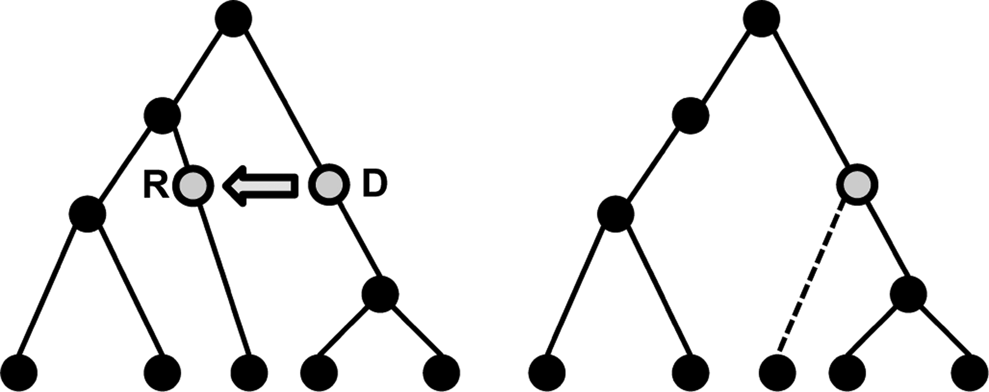
An LGT event. On the left, the species phylogeny is shown with the donor (D) and recipient (R) locations. On the right, the resulting (unweighted) gene tree is shown after the LGT transfer.

Definition 3 (Random LGT)

Let 0 < R ≤ +∞ possibly depending on n (i.e., not necessarily a constant), and note that we explicitly allow R=+∞. Let T_s=(V_s, E_s, L_s; r, τ) be a fixed species phylogeny. Let 0 < p ≤ 1 be a sampling effort probability. A gene tree topology \documentclass{aastex}\usepackage{amsbsy}\usepackage{amsfonts}\usepackage{amssymb}\usepackage{bm}\usepackage{mathrsfs}\usepackage{pifont}\usepackage{stmaryrd}\usepackage{textcomp}\usepackage{portland, xspace}\usepackage{amsmath, amsxtra}\pagestyle{empty}\DeclareMathSizes{10}{9}{7}{6}\begin{document} $${ \cal T}_g$$ \end{document} is generated according to the following continuous-time stochastic process, which gradually modifies the species phylogeny starting at the root. There are two components to the process:

1. LGT locations. The recipient and donor locations of LGT events are selected as follows:

• Recipient locations. Starting from the root, along each branch e of T_s, locations are selected as recipient of a genetic tranfer according to a continuous-time Poisson process with rate λ(e). Equivalently, the total number of LGT events is Poisson with mean Λ_tot and each such event is located independently according to the following density. For a location x on branch e, the density at x is Λ(e)/Λ_tot.

• Donor locations. If x is selected as a recipient location, the corresponding donor location y is chosen uniformly at random in \documentclass{aastex}\usepackage{amsbsy}\usepackage{amsfonts}\usepackage{amssymb}\usepackage{bm}\usepackage{mathrsfs}\usepackage{pifont}\usepackage{stmaryrd}\usepackage{textcomp}\usepackage{portland, xspace}\usepackage{amsmath, amsxtra}\pagestyle{empty}\DeclareMathSizes{10}{9}{7}{6}\begin{document} $${ \cal C}_x^{ ( R ) }$$ \end{document} . The LGT transfer is then obtained by performing an SPR move from x to y; that is, the subtree below x in T_s is moved to y in T_g. Note that we perform genetic transfers chronologically from the root.

2. Taxon sampling. Each extant leaf is kept independently with probability p. (One could also consider a different probability for each leaf. We use a fixed sampling effort p for simplicity.) The set of leaves selected is denoted by L_g. The final gene tree T_g is then obtained by keeping the subtree restricted to L_g.

The resulting (random) gene tree topology is denoted by \documentclass{aastex}\usepackage{amsbsy}\usepackage{amsfonts}\usepackage{amssymb}\usepackage{bm}\usepackage{mathrsfs}\usepackage{pifont}\usepackage{stmaryrd}\usepackage{textcomp}\usepackage{portland, xspace}\usepackage{amsmath, amsxtra}\pagestyle{empty}\DeclareMathSizes{10}{9}{7}{6}\begin{document} $${ \cal T}_g$$ \end{document} .

When R < +∞, a transfer can only occur between sufficiently closely related species. One could also consider more general donor location distributions (see e.g., Puigbo et al., 2010). In Section 4, we consider a different form of preferential exchange, highways of gene sharing.

2.2. Recovering the treelike trend: Main results

Problem statement

Let T_s=(V_s, E_s, L_s; r, τ) be an unknown species phylogeny. Using homologous gene sequences for every gene at hand, we generate N independent gene tree topologies \documentclass{aastex}\usepackage{amsbsy}\usepackage{amsfonts}\usepackage{amssymb}\usepackage{bm}\usepackage{mathrsfs}\usepackage{pifont}\usepackage{stmaryrd}\usepackage{textcomp}\usepackage{portland, xspace}\usepackage{amsmath, amsxtra}\pagestyle{empty}\DeclareMathSizes{10}{9}{7}{6}\begin{document} $${ \cal T}_{ g_1} , \ldots , { \cal T}_{ g_N}$$ \end{document} as above. Given the gene trees (or their topologies), we seek to reconstruct the topology \documentclass{aastex}\usepackage{amsbsy}\usepackage{amsfonts}\usepackage{amssymb}\usepackage{bm}\usepackage{mathrsfs}\usepackage{pifont}\usepackage{stmaryrd}\usepackage{textcomp}\usepackage{portland, xspace}\usepackage{amsmath, amsxtra}\pagestyle{empty}\DeclareMathSizes{10}{9}{7}{6}\begin{document} $${ \cal T}_s^ {+} = { \cal T} [ T_s^ {+} ]$$ \end{document} of the extant phylogeny \documentclass{aastex}\usepackage{amsbsy}\usepackage{amsfonts}\usepackage{amssymb}\usepackage{bm}\usepackage{mathrsfs}\usepackage{pifont}\usepackage{stmaryrd}\usepackage{textcomp}\usepackage{portland, xspace}\usepackage{amsmath, amsxtra}\pagestyle{empty}\DeclareMathSizes{10}{9}{7}{6}\begin{document} $$T_s^+$$ \end{document} . More precisely, we are interested in the amount of LGT that can be sustained without obscuring the phylogenetic signal. To derive asymptotic results about this question, we make some assumptions about the underlying phylogeny. We discuss two cases in detail.

In practice, one estimates gene trees from sequence data. We come back to gene tree estimation issues below.

Bounded-rates model

The following assumption was introduced in Daskalakis and Roch (2010) and is related to a common assumption in the mathematical phylogenetics literature.

Definition 4 (Bounded-rates model)

Let 0 < ρλ < 1 and 0 < ρτ < 1 be constants. Let further \documentclass{aastex}\usepackage{amsbsy}\usepackage{amsfonts}\usepackage{amssymb}\usepackage{bm}\usepackage{mathrsfs}\usepackage{pifont}\usepackage{stmaryrd}\usepackage{textcomp}\usepackage{portland, xspace}\usepackage{amsmath, amsxtra}\pagestyle{empty}\DeclareMathSizes{10}{9}{7}{6}\begin{document} $$0 < \overline { \tau} < +\:\:\: \infty$$ \end{document} be a constant and \documentclass{aastex}\usepackage{amsbsy}\usepackage{amsfonts}\usepackage{amssymb}\usepackage{bm}\usepackage{mathrsfs}\usepackage{pifont}\usepackage{stmaryrd}\usepackage{textcomp}\usepackage{portland, xspace}\usepackage{amsmath, amsxtra}\pagestyle{empty}\DeclareMathSizes{10}{9}{7}{6}\begin{document} $$0 < \overline { \lambda} < + \infty$$ \end{document} be a value possibly depending on n⁺. Under the bounded-rates model, we consider the set of phylogenies T_s=(V_s, E_s, L_s; r, τ) with n⁺ > 0 extant leaves and n⁻ ≥ 0 extinct leaves and extant phylogeny \documentclass{aastex}\usepackage{amsbsy}\usepackage{amsfonts}\usepackage{amssymb}\usepackage{bm}\usepackage{mathrsfs}\usepackage{pifont}\usepackage{stmaryrd}\usepackage{textcomp}\usepackage{portland, xspace}\usepackage{amsmath, amsxtra}\pagestyle{empty}\DeclareMathSizes{10}{9}{7}{6}\begin{document} $$T_s^+ = ( V_s^+ , E_s^+ , L_s^+;r , \tau^+ )$$ \end{document} such that the following conditions are satisfied: \documentclass{aastex}\usepackage{amsbsy}\usepackage{amsfonts}\usepackage{amssymb}\usepackage{bm}\usepackage{mathrsfs}\usepackage{pifont}\usepackage{stmaryrd}\usepackage{textcomp}\usepackage{portland, xspace}\usepackage{amsmath, amsxtra}\pagestyle{empty}\DeclareMathSizes{10}{9}{7}{6}\begin{document} \begin{align*}{ \underline \lambda} \equiv \rho_{ \lambda} \overline { \lambda} \leq \lambda ( e ) \leq \overline { \lambda} , \quad \forall e \in E_s ,\end{align*} \end{document}

and \documentclass{aastex}\usepackage{amsbsy}\usepackage{amsfonts}\usepackage{amssymb}\usepackage{bm}\usepackage{mathrsfs}\usepackage{pifont}\usepackage{stmaryrd}\usepackage{textcomp}\usepackage{portland, xspace}\usepackage{amsmath, amsxtra}\pagestyle{empty}\DeclareMathSizes{10}{9}{7}{6}\begin{document} \begin{align*}{ \underline \tau} \equiv \rho_{ \tau} \overline { \tau} \leq \tau^ {+} ( e^ {+} ) \leq \overline { \tau} , \quad \forall e^+ \in E_s^ {+} .\end{align*} \end{document}

Our result in this case follows. We use \documentclass{aastex}\usepackage{amsbsy}\usepackage{amsfonts}\usepackage{amssymb}\usepackage{bm}\usepackage{mathrsfs}\usepackage{pifont}\usepackage{stmaryrd}\usepackage{textcomp}\usepackage{portland, xspace}\usepackage{amsmath, amsxtra}\pagestyle{empty}\DeclareMathSizes{10}{9}{7}{6}\begin{document} $$\overline { \lambda}$$ \end{document} to control the amount of LGT in the model.

Theorem 1 (Main result: Bounded-rates model, R=+∞)

Let R=+∞. Under the Bounded-rates model, it is possible to reconstruct the topology of the extant phylogeny with high probability (w.h.p.) from N=Ω(log n⁺) gene tree topologies if \documentclass{aastex}\usepackage{amsbsy}\usepackage{amsfonts}\usepackage{amssymb}\usepackage{bm}\usepackage{mathrsfs}\usepackage{pifont}\usepackage{stmaryrd}\usepackage{textcomp}\usepackage{portland, xspace}\usepackage{amsmath, amsxtra}\pagestyle{empty}\DeclareMathSizes{10}{9}{7}{6}\begin{document} $$\overline { \lambda}$$ \end{document} is such that \documentclass{aastex}\usepackage{amsbsy}\usepackage{amsfonts}\usepackage{amssymb}\usepackage{bm}\usepackage{mathrsfs}\usepackage{pifont}\usepackage{stmaryrd}\usepackage{textcomp}\usepackage{portland, xspace}\usepackage{amsmath, amsxtra}\pagestyle{empty}\DeclareMathSizes{10}{9}{7}{6}\begin{document} \begin{align*} { \bold \Lambda } = O \left( { \frac { n^ { + } } { \log n^ { + } } } \right).\end{align*} \end{document}

In words, we can reconstruct the species phylogeny w.h.p. as long as the expected number of LGT events Λ (as measured on the extant phylogeny) per gene is at most of the order of \documentclass{aastex}\usepackage{amsbsy}\usepackage{amsfonts}\usepackage{amssymb}\usepackage{bm}\usepackage{mathrsfs}\usepackage{pifont}\usepackage{stmaryrd}\usepackage{textcomp}\usepackage{portland, xspace}\usepackage{amsmath, amsxtra}\pagestyle{empty}\DeclareMathSizes{10}{9}{7}{6}\begin{document} $$ { \frac { n^ { + } } { \log n^ { + } } } $$ \end{document} . This result is based on a polynomial-time algorithm we describe in Section 3. Note that, in typical phylogenomic studies, the number of genes is much larger than the number of species. Therefore, our assumption that the number of genes should be at least of the order of the logarithm of the number of extant species is mild.

We also show that the bound on Λ in Theorem 1 is close to optimal, up to logarithmic factors.

Theorem 2 (Non-recoverability)

Under the bounded-rates model, as above, with N=O(log n⁺), the topology of the extant phylogeny cannot, in general, be reconstructed w.h.p. if \documentclass{aastex}\usepackage{amsbsy}\usepackage{amsfonts}\usepackage{amssymb}\usepackage{bm}\usepackage{mathrsfs}\usepackage{pifont}\usepackage{stmaryrd}\usepackage{textcomp}\usepackage{portland, xspace}\usepackage{amsmath, amsxtra}\pagestyle{empty}\DeclareMathSizes{10}{9}{7}{6}\begin{document} $$\overline { \lambda}$$ \end{document} is such that Λ=Ω(n⁺ log log n⁺).

More generally, the species phylogeny cannot be reconstructed from N genes if Λ=Ω(n⁺ log N). Theorem 2 is proved by a coupling argument (Lindvall, 1992). In words we show that, with the order of Ω(n⁺ log log n⁺) expected LGT events, there is insufficient signal from the gene trees to distinguish between two species phylogenies with high probability.

Yule process Branching processes are commonly used to model species phylogenies (Rannala and Yang, 1996). In the continuous-time Yule process (or pure-birth process), one starts with two species (representing the two branches emanating from the root). At any given time, each species generates a new offspring at rate 0 < ν < +∞. We stop the process when the number of species is exactly n + 1 (and ignore the n + 1st species). This process generates a species phylogeny with n=n⁺ extant species with branch lengths given by the interspeciation times in the above process. Note that n⁻=0 by construction. Let 0 < ρ λ < 1 be a constant. We also assume that \documentclass{aastex}\usepackage{amsbsy}\usepackage{amsfonts}\usepackage{amssymb}\usepackage{bm}\usepackage{mathrsfs}\usepackage{pifont}\usepackage{stmaryrd}\usepackage{textcomp}\usepackage{portland, xspace}\usepackage{amsmath, amsxtra}\pagestyle{empty}\DeclareMathSizes{10}{9}{7}{6}\begin{document} \begin{align*}{ \underline \lambda} \equiv \rho_{ \lambda} \overline { \lambda} \leq \lambda ( e ) \leq \overline { \lambda} , \quad \forall e \in E_s ,\end{align*} \end{document}

for some \documentclass{aastex}\usepackage{amsbsy}\usepackage{amsfonts}\usepackage{amssymb}\usepackage{bm}\usepackage{mathrsfs}\usepackage{pifont}\usepackage{stmaryrd}\usepackage{textcomp}\usepackage{portland, xspace}\usepackage{amsmath, amsxtra}\pagestyle{empty}\DeclareMathSizes{10}{9}{7}{6}\begin{document} $$0 < \overline { \lambda} < + \infty$$ \end{document} , possibly depending on n. As above, we use \documentclass{aastex}\usepackage{amsbsy}\usepackage{amsfonts}\usepackage{amssymb}\usepackage{bm}\usepackage{mathrsfs}\usepackage{pifont}\usepackage{stmaryrd}\usepackage{textcomp}\usepackage{portland, xspace}\usepackage{amsmath, amsxtra}\pagestyle{empty}\DeclareMathSizes{10}{9}{7}{6}\begin{document} $$\overline { \lambda}$$ \end{document} to control the amount of LGT in the model.

An advantage of the Yule model is that, unlike the bounded-rates model, it does not place arbitrary constraints on the interspeciation times. In particular, the following analog of Theorem 1 suggests that our analysis does not rely on such constraints.

Theorem 3 (Main result: Yule process, R=+∞)

Let R=+∞. Under the Yule model, the following holds with probability arbitrarily close to 1. It is possible to reconstruct the topology of the extant phylogeny w.h.p. from N=Ω(log n) gene tree topologies if \documentclass{aastex}\usepackage{amsbsy}\usepackage{amsfonts}\usepackage{amssymb}\usepackage{bm}\usepackage{mathrsfs}\usepackage{pifont}\usepackage{stmaryrd}\usepackage{textcomp}\usepackage{portland, xspace}\usepackage{amsmath, amsxtra}\pagestyle{empty}\DeclareMathSizes{10}{9}{7}{6}\begin{document} $$\overline { \lambda}$$ \end{document} is such that \documentclass{aastex}\usepackage{amsbsy}\usepackage{amsfonts}\usepackage{amssymb}\usepackage{bm}\usepackage{mathrsfs}\usepackage{pifont}\usepackage{stmaryrd}\usepackage{textcomp}\usepackage{portland, xspace}\usepackage{amsmath, amsxtra}\pagestyle{empty}\DeclareMathSizes{10}{9}{7}{6}\begin{document} \begin{align*}\bold \Lambda = O \left( { \frac { n } { \log n } } \right).\end{align*} \end{document}

Preferential LGT When R < +∞, that is, when transfers occur only between sufficiently related species, we obtain the following generalization, which implies that preferential LGT makes the tree-building problem easier.

Theorem 4 (Preferential LGT)

Let 0 < R < log n⁺ possibly depending on n⁺. Under the bounded-rates model, it is possible to reconstruct the topology of the extant phylogeny w.h.p. from N=Ω(log n⁺) gene tree topologies if \documentclass{aastex}\usepackage{amsbsy}\usepackage{amsfonts}\usepackage{amssymb}\usepackage{bm}\usepackage{mathrsfs}\usepackage{pifont}\usepackage{stmaryrd}\usepackage{textcomp}\usepackage{portland, xspace}\usepackage{amsmath, amsxtra}\pagestyle{empty}\DeclareMathSizes{10}{9}{7}{6}\begin{document} $$\overline { \lambda}$$ \end{document} is such that \documentclass{aastex}\usepackage{amsbsy}\usepackage{amsfonts}\usepackage{amssymb}\usepackage{bm}\usepackage{mathrsfs}\usepackage{pifont}\usepackage{stmaryrd}\usepackage{textcomp}\usepackage{portland, xspace}\usepackage{amsmath, amsxtra}\pagestyle{empty}\DeclareMathSizes{10}{9}{7}{6}\begin{document} \begin{align*}\bold \Lambda = O \left( { \frac { n^ { + } } { R } } \right) .\end{align*} \end{document}

A similar result holds under the Yule model.

Further results

We also obtain results on highways of LGT as well as sequence-length requirements. These results require additional background. See Sections 4 and 5 respectively.

3. Probabilistic Analysis

We assume that we are given N independent gene tree topologies \documentclass{aastex}\usepackage{amsbsy}\usepackage{amsfonts}\usepackage{amssymb}\usepackage{bm}\usepackage{mathrsfs}\usepackage{pifont}\usepackage{stmaryrd}\usepackage{textcomp}\usepackage{portland, xspace}\usepackage{amsmath, amsxtra}\pagestyle{empty}\DeclareMathSizes{10}{9}{7}{6}\begin{document} $${ \cal T}_{ g_1} , \ldots , { \cal T}_{ g_N}$$ \end{document} as above. Our goal is to reconstruct the extant phylogeny.

Different algorithms are possible. A simple approach is to take a majority vote over all gene-tree topologies. But this approach is problematic under taxon sampling and cannot sustain the high levels of LGT we consider below.

Instead, we consider approaches that aggregate partial information over all gene trees. We focus on subtrees over four taxa whose topologies are called quartets (Semple and Steel, 2003). We show that computationally efficient quartet-based approaches can sustain high levels of LGT. Although we prove our results for the specific method described below, our analysis is likely to apply to related methods. In Section 5.1, we also give a similar analysis for a distance-based method of Kim and Salisbury (2001).

3.1. Algorithm

We consider the following approach related to an algorithm of Zhaxybayeva et al. (2006). Let X={a, b, c, d} be a four-tuple of extant species. The topology \documentclass{aastex}\usepackage{amsbsy}\usepackage{amsfonts}\usepackage{amssymb}\usepackage{bm}\usepackage{mathrsfs}\usepackage{pifont}\usepackage{stmaryrd}\usepackage{textcomp}\usepackage{portland, xspace}\usepackage{amsmath, amsxtra}\pagestyle{empty}\DeclareMathSizes{10}{9}{7}{6}\begin{document} $${ \cal T} \mid X$$ \end{document} of a tree \documentclass{aastex}\usepackage{amsbsy}\usepackage{amsfonts}\usepackage{amssymb}\usepackage{bm}\usepackage{mathrsfs}\usepackage{pifont}\usepackage{stmaryrd}\usepackage{textcomp}\usepackage{portland, xspace}\usepackage{amsmath, amsxtra}\pagestyle{empty}\DeclareMathSizes{10}{9}{7}{6}\begin{document} $${ \cal T}$$ \end{document} restricted to X can be summarized with a quartet split, or quartet for short. There are three possible (resolved) quartets that we denote q₁=ab|cd, q₂=ac|bd, and q₃=ad|bc. We first compute the frequency of each quartet over all gene trees displaying X, that is, over all gene trees g such that X ⊆ L_g, \documentclass{aastex}\usepackage{amsbsy}\usepackage{amsfonts}\usepackage{amssymb}\usepackage{bm}\usepackage{mathrsfs}\usepackage{pifont}\usepackage{stmaryrd}\usepackage{textcomp}\usepackage{portland, xspace}\usepackage{amsmath, amsxtra}\pagestyle{empty}\DeclareMathSizes{10}{9}{7}{6}\begin{document} \begin{align*}f_X ( q_1 ) = { \frac { \mid \ { g_i : X \subseteq L_ { g_i } , \ { \cal T } _ { g_i } \mid X = q_1 \ } \mid } { \mid \ { g_i : X \subseteq L_ { g_i } \ } \mid } } ,\end{align*} \end{document}

and similarly for q₂, q₃. (We set the frequency to 0 if the denominator is 0.) For each X, we choose the quartet with highest frequency (breaking ties arbitrarily).

Definition 5

A set of quartets Q={q_i}, with L_qi the leaf set of q_i, is compatible if there is a tree \documentclass{aastex}\usepackage{amsbsy}\usepackage{amsfonts}\usepackage{amssymb}\usepackage{bm}\usepackage{mathrsfs}\usepackage{pifont}\usepackage{stmaryrd}\usepackage{textcomp}\usepackage{portland, xspace}\usepackage{amsmath, amsxtra}\pagestyle{empty}\DeclareMathSizes{10}{9}{7}{6}\begin{document} $${ \cal T}$$ \end{document} with leaf set \documentclass{aastex}\usepackage{amsbsy}\usepackage{amsfonts}\usepackage{amssymb}\usepackage{bm}\usepackage{mathrsfs}\usepackage{pifont}\usepackage{stmaryrd}\usepackage{textcomp}\usepackage{portland, xspace}\usepackage{amsmath, amsxtra}\pagestyle{empty}\DeclareMathSizes{10}{9}{7}{6}\begin{document} $$L_Q \equiv \cup_{q_i \in Q} L_{q_i}$$ \end{document} such that \documentclass{aastex}\usepackage{amsbsy}\usepackage{amsfonts}\usepackage{amssymb}\usepackage{bm}\usepackage{mathrsfs}\usepackage{pifont}\usepackage{stmaryrd}\usepackage{textcomp}\usepackage{portland, xspace}\usepackage{amsmath, amsxtra}\pagestyle{empty}\DeclareMathSizes{10}{9}{7}{6}\begin{document} $${ \cal T}$$ \end{document} agrees with every q_i.

Quartet compatibility is, in general, NP-hard (Steel, 1992). However, when the set Q covers all possible four-tuple of taxa (that is, exactly \documentclass{aastex}\usepackage{amsbsy}\usepackage{amsfonts}\usepackage{amssymb}\usepackage{bm}\usepackage{mathrsfs}\usepackage{pifont}\usepackage{stmaryrd}\usepackage{textcomp}\usepackage{portland, xspace}\usepackage{amsmath, amsxtra}\pagestyle{empty}\DeclareMathSizes{10}{9}{7}{6}\begin{document} $$n \choose 4$$ \end{document} quartets with no repeated four-tuple of taxa), there is a polynomial-time algorithm for compatibility (Bandelt and Dress, 1986; Buneman, 1971; Berry and Gascuel, 2001). In our procedure, for every four-tuple of taxa, there is a single quartet chosen, so we can check compatibility easily and output the corresponding tree. In practice, if Q is not compatible, one can use instead a heuristic supertree method such as MRP (Baum, 1992; Ragan, 1992) or Quartet MaxCut (Snir and Rao, 2010, 2012).

The algorithm, which we call QuartetPlurality (QP), is detailed in Figure 2.

FIG. 2.

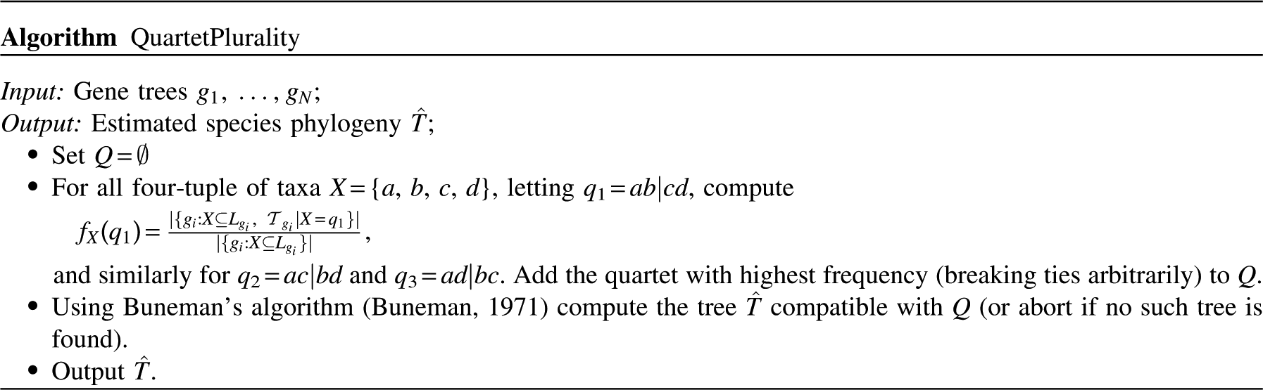
Algorithm QuartetPlurality.

3.2. A general formula

Our asymptotic analysis is based on the following claim. Recall that, for a subset of extant species X, we let \documentclass{aastex}\usepackage{amsbsy}\usepackage{amsfonts}\usepackage{amssymb}\usepackage{bm}\usepackage{mathrsfs}\usepackage{pifont}\usepackage{stmaryrd}\usepackage{textcomp}\usepackage{portland, xspace}\usepackage{amsmath, amsxtra}\pagestyle{empty}\DeclareMathSizes{10}{9}{7}{6}\begin{document} $${ \cal T} _s \mid X$$ \end{document} be the extant phylogeny topology restricted to X with corresponding edge set \documentclass{aastex}\usepackage{amsbsy}\usepackage{amsfonts}\usepackage{amssymb}\usepackage{bm}\usepackage{mathrsfs}\usepackage{pifont}\usepackage{stmaryrd}\usepackage{textcomp}\usepackage{portland, xspace}\usepackage{amsmath, amsxtra}\pagestyle{empty}\DeclareMathSizes{10}{9}{7}{6}\begin{document} $${ \cal E} ( { \cal T} _s \mid X )$$ \end{document} . Also recall that Λ(e)=λ(e)τ(e) is the expected number of LGT events on edge e, which we refer to as the LGT weight, or weight for short, of e. Let \documentclass{aastex}\usepackage{amsbsy}\usepackage{amsfonts}\usepackage{amssymb}\usepackage{bm}\usepackage{mathrsfs}\usepackage{pifont}\usepackage{stmaryrd}\usepackage{textcomp}\usepackage{portland, xspace}\usepackage{amsmath, amsxtra}\pagestyle{empty}\DeclareMathSizes{10}{9}{7}{6}\begin{document} \begin{align*}\bold \Lambda_X = \sum_{e \in { \cal E} ( { \cal T}_s \mid X ) } \bold \Lambda ( e ) ,\end{align*} \end{document}

be the total weight of the subtree \documentclass{aastex}\usepackage{amsbsy}\usepackage{amsfonts}\usepackage{amssymb}\usepackage{bm}\usepackage{mathrsfs}\usepackage{pifont}\usepackage{stmaryrd}\usepackage{textcomp}\usepackage{portland, xspace}\usepackage{amsmath, amsxtra}\pagestyle{empty}\DeclareMathSizes{10}{9}{7}{6}\begin{document} $${ \cal T}_s \mid X$$ \end{document} under the weights \documentclass{aastex}\usepackage{amsbsy}\usepackage{amsfonts}\usepackage{amssymb}\usepackage{bm}\usepackage{mathrsfs}\usepackage{pifont}\usepackage{stmaryrd}\usepackage{textcomp}\usepackage{portland, xspace}\usepackage{amsmath, amsxtra}\pagestyle{empty}\DeclareMathSizes{10}{9}{7}{6}\begin{document} $$\Lambda ( e ) , \ e \in E_s$$ \end{document} . Define the maximum quartet weight (MQW) as \documentclass{aastex}\usepackage{amsbsy}\usepackage{amsfonts}\usepackage{amssymb}\usepackage{bm}\usepackage{mathrsfs}\usepackage{pifont}\usepackage{stmaryrd}\usepackage{textcomp}\usepackage{portland, xspace}\usepackage{amsmath, amsxtra}\pagestyle{empty}\DeclareMathSizes{10}{9}{7}{6}\begin{document} \begin{align*}\bold \Upsilon^{\ ( 4 ) } = \max \{ \bold \Lambda_X : X \subseteq ( L_s^+ ) ^4 \} .\end{align*} \end{document}

Lemma 1 (Probability of a miss)

Let \documentclass{aastex}\usepackage{amsbsy}\usepackage{amsfonts}\usepackage{amssymb}\usepackage{bm}\usepackage{mathrsfs}\usepackage{pifont}\usepackage{stmaryrd}\usepackage{textcomp}\usepackage{portland, xspace}\usepackage{amsmath, amsxtra}\pagestyle{empty}\DeclareMathSizes{10}{9}{7}{6}\begin{document} $${ \cal T} _g$$ \end{document} be a gene tree topology distributed according to the random LGT model such that X={a, b, c, d} ⊆ L_g. Let \documentclass{aastex}\usepackage{amsbsy}\usepackage{amsfonts}\usepackage{amssymb}\usepackage{bm}\usepackage{mathrsfs}\usepackage{pifont}\usepackage{stmaryrd}\usepackage{textcomp}\usepackage{portland, xspace}\usepackage{amsmath, amsxtra}\pagestyle{empty}\DeclareMathSizes{10}{9}{7}{6}\begin{document} $$q_s^X$$ \end{document} (respectively \documentclass{aastex}\usepackage{amsbsy}\usepackage{amsfonts}\usepackage{amssymb}\usepackage{bm}\usepackage{mathrsfs}\usepackage{pifont}\usepackage{stmaryrd}\usepackage{textcomp}\usepackage{portland, xspace}\usepackage{amsmath, amsxtra}\pagestyle{empty}\DeclareMathSizes{10}{9}{7}{6}\begin{document} $$q_g^X$$ \end{document} ) be the quartet corresponding to \documentclass{aastex}\usepackage{amsbsy}\usepackage{amsfonts}\usepackage{amssymb}\usepackage{bm}\usepackage{mathrsfs}\usepackage{pifont}\usepackage{stmaryrd}\usepackage{textcomp}\usepackage{portland, xspace}\usepackage{amsmath, amsxtra}\pagestyle{empty}\DeclareMathSizes{10}{9}{7}{6}\begin{document} $${ \cal T}_g \mid X$$ \end{document} (respectively \documentclass{aastex}\usepackage{amsbsy}\usepackage{amsfonts}\usepackage{amssymb}\usepackage{bm}\usepackage{mathrsfs}\usepackage{pifont}\usepackage{stmaryrd}\usepackage{textcomp}\usepackage{portland, xspace}\usepackage{amsmath, amsxtra}\pagestyle{empty}\DeclareMathSizes{10}{9}{7}{6}\begin{document} $${ \cal T} _g \mid X$$ \end{document} ). Then \documentclass{aastex}\usepackage{amsbsy}\usepackage{amsfonts}\usepackage{amssymb}\usepackage{bm}\usepackage{mathrsfs}\usepackage{pifont}\usepackage{stmaryrd}\usepackage{textcomp}\usepackage{portland, xspace}\usepackage{amsmath, amsxtra}\pagestyle{empty}\DeclareMathSizes{10}{9}{7}{6}\begin{document} \begin{align*}{\mathbb P} [ q^X_g = q^X_s \mid X \subseteq L_g ] \geq \exp \left( - \Upsilon^{ ( 4 ) } \right) .\end{align*} \end{document}

Recall that Λ is the expected number of LGT events (as measured on the extant phylogeny) per gene. As a comparison, note that the probability that a gene tree is LGT-free is e^−Λ, which can be much smaller.

Proof (Lemma 1)

We first note that, by our assumption that the species phylogeny is bifurcating, \documentclass{aastex}\usepackage{amsbsy}\usepackage{amsfonts}\usepackage{amssymb}\usepackage{bm}\usepackage{mathrsfs}\usepackage{pifont}\usepackage{stmaryrd}\usepackage{textcomp}\usepackage{portland, xspace}\usepackage{amsmath, amsxtra}\pagestyle{empty}\DeclareMathSizes{10}{9}{7}{6}\begin{document} $$q_s^X$$ \end{document} is resolved. Similarly \documentclass{aastex}\usepackage{amsbsy}\usepackage{amsfonts}\usepackage{amssymb}\usepackage{bm}\usepackage{mathrsfs}\usepackage{pifont}\usepackage{stmaryrd}\usepackage{textcomp}\usepackage{portland, xspace}\usepackage{amsmath, amsxtra}\pagestyle{empty}\DeclareMathSizes{10}{9}{7}{6}\begin{document} $$q_g^X$$ \end{document} is resolved because under a Poisson process for the recipient location, the probability that a vertex has degree higher than 2 (that is, that a pruning and re-grafting occurs exactly at the location of an existing vertex) is 0.

Now we observe that if none of the recipient locations lands on \documentclass{aastex}\usepackage{amsbsy}\usepackage{amsfonts}\usepackage{amssymb}\usepackage{bm}\usepackage{mathrsfs}\usepackage{pifont}\usepackage{stmaryrd}\usepackage{textcomp}\usepackage{portland, xspace}\usepackage{amsmath, amsxtra}\pagestyle{empty}\DeclareMathSizes{10}{9}{7}{6}\begin{document} $${ \cal T}_s \mid X$$ \end{document} then the corresponding quartet remains intact. Indeed an SPR move can only (potentially) affect those quartets with at least one leaf in the pruned subtree, and this happens with probability \documentclass{aastex}\usepackage{amsbsy}\usepackage{amsfonts}\usepackage{amssymb}\usepackage{bm}\usepackage{mathrsfs}\usepackage{pifont}\usepackage{stmaryrd}\usepackage{textcomp}\usepackage{portland, xspace}\usepackage{amsmath, amsxtra}\pagestyle{empty}\DeclareMathSizes{10}{9}{7}{6}\begin{document} $$ \frac { \bold \Lambda_X } { \bold \Lambda } $$ \end{document} . The claim then follows by induction on the number of LGT events.

Hence the probability that \documentclass{aastex}\usepackage{amsbsy}\usepackage{amsfonts}\usepackage{amssymb}\usepackage{bm}\usepackage{mathrsfs}\usepackage{pifont}\usepackage{stmaryrd}\usepackage{textcomp}\usepackage{portland, xspace}\usepackage{amsmath, amsxtra}\pagestyle{empty}\DeclareMathSizes{10}{9}{7}{6}\begin{document} $$q_g^X = q_s^X$$ \end{document} is at least the probability that all LGT events (on the extant phylogeny) miss \documentclass{aastex}\usepackage{amsbsy}\usepackage{amsfonts}\usepackage{amssymb}\usepackage{bm}\usepackage{mathrsfs}\usepackage{pifont}\usepackage{stmaryrd}\usepackage{textcomp}\usepackage{portland, xspace}\usepackage{amsmath, amsxtra}\pagestyle{empty}\DeclareMathSizes{10}{9}{7}{6}\begin{document} $${ \cal T} _s \mid X$$ \end{document} , which is at least \documentclass{aastex}\usepackage{amsbsy}\usepackage{amsfonts}\usepackage{amssymb}\usepackage{bm}\usepackage{mathrsfs}\usepackage{pifont}\usepackage{stmaryrd}\usepackage{textcomp}\usepackage{portland, xspace}\usepackage{amsmath, amsxtra}\pagestyle{empty}\DeclareMathSizes{10}{9}{7}{6}\begin{document} \begin{align*} { \mathbb P } [ q^X_g = q^X_s \mid X \subseteq L_g ] & \geq \sum_ { i = 0 } ^ { + \infty } { \frac { e^ { - \bold \Lambda } \bold \Lambda^i } { i! } } \left( 1 - { \frac { \bold \Lambda_X } { \bold \Lambda } } \right) ^i \\ & = e^ { - \bold \Lambda } \exp \left( \bold \Lambda \left( 1 - { \frac { \bold \Lambda_X } { \bold \Lambda } } \right) \right) \\ & \geq \exp \left( - \Upsilon^ { \; ( 4 ) } \right) . \end{align*} \end{document} ■

3.3. Bounded-rates and Yule models

Next we argue that, under appropriate assumptions on the species phylogeny, the maximum quartet weight is bounded in such a way that the plurality quartet topology for every four-tuple of taxa X={a, b, c, d}, which we denote by \documentclass{aastex}\usepackage{amsbsy}\usepackage{amsfonts}\usepackage{amssymb}\usepackage{bm}\usepackage{mathrsfs}\usepackage{pifont}\usepackage{stmaryrd}\usepackage{textcomp}\usepackage{portland, xspace}\usepackage{amsmath, amsxtra}\pagestyle{empty}\DeclareMathSizes{10}{9}{7}{6}\begin{document} $$q_*^X$$ \end{document} , satisfies \documentclass{aastex}\usepackage{amsbsy}\usepackage{amsfonts}\usepackage{amssymb}\usepackage{bm}\usepackage{mathrsfs}\usepackage{pifont}\usepackage{stmaryrd}\usepackage{textcomp}\usepackage{portland, xspace}\usepackage{amsmath, amsxtra}\pagestyle{empty}\DeclareMathSizes{10}{9}{7}{6}\begin{document} $$q_*^X = q_s^X$$ \end{document} . As a result, our quartet set is compatible and \documentclass{aastex}\usepackage{amsbsy}\usepackage{amsfonts}\usepackage{amssymb}\usepackage{bm}\usepackage{mathrsfs}\usepackage{pifont}\usepackage{stmaryrd}\usepackage{textcomp}\usepackage{portland, xspace}\usepackage{amsmath, amsxtra}\pagestyle{empty}\DeclareMathSizes{10}{9}{7}{6}\begin{document} $${ \cal T} _s^ {+}$$ \end{document} can be reconstructed efficiently.

3.3.1. Bounded-rates model

We bound the maximum quartet weight ϒ⁽⁴⁾ in the bounded-rates model.

Lemma 2 (Bound on quartet weight: Bounded-rates case)

Under the Bounded-rates model, it holds that \documentclass{aastex}\usepackage{amsbsy}\usepackage{amsfonts}\usepackage{amssymb}\usepackage{bm}\usepackage{mathrsfs}\usepackage{pifont}\usepackage{stmaryrd}\usepackage{textcomp}\usepackage{portland, xspace}\usepackage{amsmath, amsxtra}\pagestyle{empty}\DeclareMathSizes{10}{9}{7}{6}\begin{document} \begin{align*}\Upsilon^{ ( 4 ) } = O \left( \overline { \lambda} \log n^ {+} \right) , \qquad \bold \Lambda = \Theta ( \overline { \lambda} n^ {+} ) .\end{align*} \end{document}

Proof (Lemma 2)

The first part of the proof is taken from Daskalakis and Roch (2010). Let h (respectively H) be the smallest (respectively largest) number of edges on a path between the root and an extant leaf. Because the number of extant leaves is n⁺ and the extant phylogeny is bifurcating (recall that we suppressed vertices of degree 2 after taking a restriction to the extant species), we must have 2^h ≤ n⁺ and 2^H ≥ n⁺. Since all extant leaves are contemporaneous it must be that \documentclass{aastex}\usepackage{amsbsy}\usepackage{amsfonts}\usepackage{amssymb}\usepackage{bm}\usepackage{mathrsfs}\usepackage{pifont}\usepackage{stmaryrd}\usepackage{textcomp}\usepackage{portland, xspace}\usepackage{amsmath, amsxtra}\pagestyle{empty}\DeclareMathSizes{10}{9}{7}{6}\begin{document} $$H \underline { \tau} \leq h \overline { \tau}$$ \end{document} . Combining these constraints gives \documentclass{aastex}\usepackage{amsbsy}\usepackage{amsfonts}\usepackage{amssymb}\usepackage{bm}\usepackage{mathrsfs}\usepackage{pifont}\usepackage{stmaryrd}\usepackage{textcomp}\usepackage{portland, xspace}\usepackage{amsmath, amsxtra}\pagestyle{empty}\DeclareMathSizes{10}{9}{7}{6}\begin{document} \begin{align*} { \frac { \underline { \tau } } { \overline { \tau } } } \log_2 n^ { + } \leq h \leq H \leq { \frac {\overline { \tau } } { \underline { \tau } } } \log_2 n^ { + } .\end{align*} \end{document}

Hence \documentclass{aastex}\usepackage{amsbsy}\usepackage{amsfonts}\usepackage{amssymb}\usepackage{bm}\usepackage{mathrsfs}\usepackage{pifont}\usepackage{stmaryrd}\usepackage{textcomp}\usepackage{portland, xspace}\usepackage{amsmath, amsxtra}\pagestyle{empty}\DeclareMathSizes{10}{9}{7}{6}\begin{document} \begin{align*}\max \{ {\bold \Lambda}_X : X \subseteq ( L_s^ { + } ) ^4 \} \leq 4 {\overline { \lambda } } { \overline{ \tau }} { \frac{ \overline{ \tau } } { \underline { \tau } } } \log_2 n^ { + } . \end{align*} \end{document}

The total number of edges in the extant phylogeny is 2n⁺ − 3 so that \documentclass{aastex}\usepackage{amsbsy}\usepackage{amsfonts}\usepackage{amssymb}\usepackage{bm}\usepackage{mathrsfs}\usepackage{pifont}\usepackage{stmaryrd}\usepackage{textcomp}\usepackage{portland, xspace}\usepackage{amsmath, amsxtra}\pagestyle{empty}\DeclareMathSizes{10}{9}{7}{6}\begin{document} \begin{align*}{\bold \Lambda} = \Theta ( \overline { \lambda} n^ {+} ).\end{align*} \end{document}

Using Lemma 2, we prove Theorem 1. First recall the following standard concentration inequality (see, e.g., Motwani and Raghavan, 1995):

Lemma 3 (Azuma-Hoeffding inequality)

Suppose \documentclass{aastex}\usepackage{amsbsy}\usepackage{amsfonts}\usepackage{amssymb}\usepackage{bm}\usepackage{mathrsfs}\usepackage{pifont}\usepackage{stmaryrd}\usepackage{textcomp}\usepackage{portland, xspace}\usepackage{amsmath, amsxtra}\pagestyle{empty}\DeclareMathSizes{10}{9}{7}{6}\begin{document} $${ \bf Z} = ( Z_1 , \ldots , Z_m )$$ \end{document} are independent random variables taking values in a set S, and \documentclass{aastex}\usepackage{amsbsy}\usepackage{amsfonts}\usepackage{amssymb}\usepackage{bm}\usepackage{mathrsfs}\usepackage{pifont}\usepackage{stmaryrd}\usepackage{textcomp}\usepackage{portland, xspace}\usepackage{amsmath, amsxtra}\pagestyle{empty}\DeclareMathSizes{10}{9}{7}{6}\begin{document} $$h \ : \ S^m \rightarrow {\mathbb R}$$ \end{document} is any t-Lipschitz function: |h(z) − h(z′)| ≤ t whenever \documentclass{aastex}\usepackage{amsbsy}\usepackage{amsfonts}\usepackage{amssymb}\usepackage{bm}\usepackage{mathrsfs}\usepackage{pifont}\usepackage{stmaryrd}\usepackage{textcomp}\usepackage{portland, xspace}\usepackage{amsmath, amsxtra}\pagestyle{empty}\DeclareMathSizes{10}{9}{7}{6}\begin{document} $${ \bf z} , { \bf z^{ \prime}} \in S^m$$ \end{document} differ at just one coordinate. Then, ∀ζ> 0, \documentclass{aastex}\usepackage{amsbsy}\usepackage{amsfonts}\usepackage{amssymb}\usepackage{bm}\usepackage{mathrsfs}\usepackage{pifont}\usepackage{stmaryrd}\usepackage{textcomp}\usepackage{portland, xspace}\usepackage{amsmath, amsxtra}\pagestyle{empty}\DeclareMathSizes{10}{9}{7}{6}\begin{document} \begin{align*} { \mathbb P } \left[ \mid h ( { \bf Z } ) - { \mathbb E } [ h ( { \bf Z } ) ] \mid \geq \zeta \right] \leq 2 \exp \left( - { \frac { \zeta^2 } { 2 t^2 m } } \right) .\end{align*} \end{document}

Proof (Theorem 1)

Consider the quartet-based approach described in Section 3.1. Take \documentclass{aastex}\usepackage{amsbsy}\usepackage{amsfonts}\usepackage{amssymb}\usepackage{bm}\usepackage{mathrsfs}\usepackage{pifont}\usepackage{stmaryrd}\usepackage{textcomp}\usepackage{portland, xspace}\usepackage{amsmath, amsxtra}\pagestyle{empty}\DeclareMathSizes{10}{9}{7}{6}\begin{document} $$\overline { \lambda} = C_1 / \log n^ {+}$$ \end{document} with C₁ > 0 small enough so that \documentclass{aastex}\usepackage{amsbsy}\usepackage{amsfonts}\usepackage{amssymb}\usepackage{bm}\usepackage{mathrsfs}\usepackage{pifont}\usepackage{stmaryrd}\usepackage{textcomp}\usepackage{portland, xspace}\usepackage{amsmath, amsxtra}\pagestyle{empty}\DeclareMathSizes{10}{9}{7}{6}\begin{document} \begin{align*}\bold \Lambda = O \left( { \frac { n^ { + } } { \log n^ { + } } } \right) ,\end{align*} \end{document}

and using Lemmas 1 and 2, we have for any four-tuple X of extant species \documentclass{aastex}\usepackage{amsbsy}\usepackage{amsfonts}\usepackage{amssymb}\usepackage{bm}\usepackage{mathrsfs}\usepackage{pifont}\usepackage{stmaryrd}\usepackage{textcomp}\usepackage{portland, xspace}\usepackage{amsmath, amsxtra}\pagestyle{empty}\DeclareMathSizes{10}{9}{7}{6}\begin{document} \begin{align*}{\mathbb P} [ X \subseteq L_g ] = p^4 ,\end{align*} \end{document}

and \documentclass{aastex}\usepackage{amsbsy}\usepackage{amsfonts}\usepackage{amssymb}\usepackage{bm}\usepackage{mathrsfs}\usepackage{pifont}\usepackage{stmaryrd}\usepackage{textcomp}\usepackage{portland, xspace}\usepackage{amsmath, amsxtra}\pagestyle{empty}\DeclareMathSizes{10}{9}{7}{6}\begin{document} \begin{align*} { \mathbb P } [ q^X_g = q^X_s \ \mid \ X \subseteq L_g ] \geq \exp \left( - \Upsilon^ { ( 4 ) } \right) \geq \exp \left( - O ( C_1 ) \right) \geq { \frac { 2 } { 3 } } ,\end{align*} \end{document}

for C₁ small enough. We choose C₂ > 0 large enough with \documentclass{aastex}\usepackage{amsbsy}\usepackage{amsfonts}\usepackage{amssymb}\usepackage{bm}\usepackage{mathrsfs}\usepackage{pifont}\usepackage{stmaryrd}\usepackage{textcomp}\usepackage{portland, xspace}\usepackage{amsmath, amsxtra}\pagestyle{empty}\DeclareMathSizes{10}{9}{7}{6}\begin{document} \begin{align*}N \geq C_2 \log n^ {+} ,\end{align*} \end{document}

and ɛ < p⁴ so that, using Lemma 3, the following inequalities hold. Consider the following events \documentclass{aastex}\usepackage{amsbsy}\usepackage{amsfonts}\usepackage{amssymb}\usepackage{bm}\usepackage{mathrsfs}\usepackage{pifont}\usepackage{stmaryrd}\usepackage{textcomp}\usepackage{portland, xspace}\usepackage{amsmath, amsxtra}\pagestyle{empty}\DeclareMathSizes{10}{9}{7}{6}\begin{document} \begin{align*}{ \cal E}_0 = \{ \mid \mid \{ g_i : X \subseteq L_{g_i} \} \mid - N p^4 \mid \leq N \varepsilon \} \end{align*} \end{document}

and \documentclass{aastex}\usepackage{amsbsy}\usepackage{amsfonts}\usepackage{amssymb}\usepackage{bm}\usepackage{mathrsfs}\usepackage{pifont}\usepackage{stmaryrd}\usepackage{textcomp}\usepackage{portland, xspace}\usepackage{amsmath, amsxtra}\pagestyle{empty}\DeclareMathSizes{10}{9}{7}{6}\begin{document} \begin{align*} { \cal E } _1 = \left\{ \mid \{ g_i : X \subseteq L_ { g_i } , \ { \cal T } _ { g_i } \mid X = q_1 \} \mid > \frac { 1 } { 2 } \mid \{ g_i : X \subseteq L_ { g_i } \} \mid \right\} .\end{align*} \end{document}

By Lemma 3, \documentclass{aastex}\usepackage{amsbsy}\usepackage{amsfonts}\usepackage{amssymb}\usepackage{bm}\usepackage{mathrsfs}\usepackage{pifont}\usepackage{stmaryrd}\usepackage{textcomp}\usepackage{portland, xspace}\usepackage{amsmath, amsxtra}\pagestyle{empty}\DeclareMathSizes{10}{9}{7}{6}\begin{document} \begin{align*}{\mathbb P} [ { \cal E}_0^c ] \leq \exp \left( - O ( \varepsilon^2 N ) \right) ,\end{align*} \end{document}

and \documentclass{aastex}\usepackage{amsbsy}\usepackage{amsfonts}\usepackage{amssymb}\usepackage{bm}\usepackage{mathrsfs}\usepackage{pifont}\usepackage{stmaryrd}\usepackage{textcomp}\usepackage{portland, xspace}\usepackage{amsmath, amsxtra}\pagestyle{empty}\DeclareMathSizes{10}{9}{7}{6}\begin{document} \begin{align*}{\mathbb P} [ { \cal E}_1^c \ \mid \ { \cal E}_0 ] \leq \exp \left( - O ( N ( p^4 - \varepsilon ) ) \right) .\end{align*} \end{document}

Hence, for a constant C₂ large enough, \documentclass{aastex}\usepackage{amsbsy}\usepackage{amsfonts}\usepackage{amssymb}\usepackage{bm}\usepackage{mathrsfs}\usepackage{pifont}\usepackage{stmaryrd}\usepackage{textcomp}\usepackage{portland, xspace}\usepackage{amsmath, amsxtra}\pagestyle{empty}\DeclareMathSizes{10}{9}{7}{6}\begin{document} \begin{align*} { \mathbb P } [ f_X ( q^X_s ) < 1 / 2 ] & \leq { \mathbb P } [ { \cal E } _0^c ] + { \mathbb P } [ { \cal E } _1^c \mid { \cal E } _0 ] \\ & \leq O \left( \frac { 1 } { ( n^ { + } ) ^4 } \right) . \end{align*} \end{document}

Then the plurality vote is correct for every four-tuple of taxa, and the extant phylogeny is correctly reconstructed. ■

3.3.2. Yule process

We now consider the Yule model.

Lemma 4 (Bound on quartet weight: Yule case)

Under the Yule model, it holds that \documentclass{aastex}\usepackage{amsbsy}\usepackage{amsfonts}\usepackage{amssymb}\usepackage{bm}\usepackage{mathrsfs}\usepackage{pifont}\usepackage{stmaryrd}\usepackage{textcomp}\usepackage{portland, xspace}\usepackage{amsmath, amsxtra}\pagestyle{empty}\DeclareMathSizes{10}{9}{7}{6}\begin{document} \begin{align*}\Upsilon^{ ( 4 ) } = \Theta \left( \overline \lambda \log n \right) , \qquad \bold \Lambda = \Theta \left( \overline \lambda n \right)\end{align*} \end{document}

with probability approaching 1 as n → +∞.

Proof (Lemma 4)

We consider a pure-birth process with birth rate ν starting from two species. For background on branching processes, see Athreya and Ney (1972).

Let Z_i be the (i − 1)-th interspeciation time. As a minimum of i independent exponential distributions with mean 1/ν, Z_i is an exponential with mean 1/ (iν). Moreover, the Z_is are independent. Hence the height of the phylogeny in time units, that is, the total time until n + 1 species are present [recall that we ignore the (n + 1)-st species] is \documentclass{aastex}\usepackage{amsbsy}\usepackage{amsfonts}\usepackage{amssymb}\usepackage{bm}\usepackage{mathrsfs}\usepackage{pifont}\usepackage{stmaryrd}\usepackage{textcomp}\usepackage{portland, xspace}\usepackage{amsmath, amsxtra}\pagestyle{empty}\DeclareMathSizes{10}{9}{7}{6}\begin{document} \begin{align*}{ \bf Z} = \sum_{i = 2}^{n + 1} Z_i ,\end{align*} \end{document}

and we have \documentclass{aastex}\usepackage{amsbsy}\usepackage{amsfonts}\usepackage{amssymb}\usepackage{bm}\usepackage{mathrsfs}\usepackage{pifont}\usepackage{stmaryrd}\usepackage{textcomp}\usepackage{portland, xspace}\usepackage{amsmath, amsxtra}\pagestyle{empty}\DeclareMathSizes{10}{9}{7}{6}\begin{document} \begin{align*} { \mathbb E } [ { \bf Z } ] = \sum_ { i = 2 } ^ { n + 1 } { \mathbb E } [ Z_i ] = \sum_ { i = 2 } ^ { n + 1 } { \frac { 1 } { i \nu } } = \Theta ( \nu^ { - 1 } \log n ) ,\end{align*} \end{document}

and \documentclass{aastex}\usepackage{amsbsy}\usepackage{amsfonts}\usepackage{amssymb}\usepackage{bm}\usepackage{mathrsfs}\usepackage{pifont}\usepackage{stmaryrd}\usepackage{textcomp}\usepackage{portland, xspace}\usepackage{amsmath, amsxtra}\pagestyle{empty}\DeclareMathSizes{10}{9}{7}{6}\begin{document} \begin{align*} { \rm Var } [ { \bf Z } ] = \sum_ { i = 2 } ^ { n + 1 } { \rm Var } [ Z_i ] = \sum_ { i = 2 } ^ { n + 1 } { \frac { 1 } { i^2 \nu^2 } } = \Theta ( \nu^ { - 2 } ) .\end{align*} \end{document}

The total weight of the phylogeny in time units \documentclass{aastex}\usepackage{amsbsy}\usepackage{amsfonts}\usepackage{amssymb}\usepackage{bm}\usepackage{mathrsfs}\usepackage{pifont}\usepackage{stmaryrd}\usepackage{textcomp}\usepackage{portland, xspace}\usepackage{amsmath, amsxtra}\pagestyle{empty}\DeclareMathSizes{10}{9}{7}{6}\begin{document} \begin{align*}{ \bf Y} = \sum_{i = 2}^{n + 1} i Z_i ,\end{align*} \end{document}

is a sum of n independent exponential random variables with parameter ν, and we have \documentclass{aastex}\usepackage{amsbsy}\usepackage{amsfonts}\usepackage{amssymb}\usepackage{bm}\usepackage{mathrsfs}\usepackage{pifont}\usepackage{stmaryrd}\usepackage{textcomp}\usepackage{portland, xspace}\usepackage{amsmath, amsxtra}\pagestyle{empty}\DeclareMathSizes{10}{9}{7}{6}\begin{document} \begin{align*} { \mathbb E } [ { \bf Y } ] = \sum_ { i = 2 } ^ { n + 1 } i { \mathbb E } [ Z_i ] = \sum_ { i = 2 } ^ { n + 1 } i { \frac { 1 } { i \nu } } = \nu^ { - 1 } n ,\end{align*} \end{document}

and \documentclass{aastex}\usepackage{amsbsy}\usepackage{amsfonts}\usepackage{amssymb}\usepackage{bm}\usepackage{mathrsfs}\usepackage{pifont}\usepackage{stmaryrd}\usepackage{textcomp}\usepackage{portland, xspace}\usepackage{amsmath, amsxtra}\pagestyle{empty}\DeclareMathSizes{10}{9}{7}{6}\begin{document} \begin{align*} { \rm Var } [ { \bf Y } ] = \sum_ { i = 2 } ^ { n + 1 } i^2 { \rm Var } [ Z_i ] = \sum_ { i = 2 } ^ { n + 1 } i^2 { \frac { 1 } { i^2 \nu^2 } } = \nu^ { - 2 } n.\end{align*} \end{document}

By Chebyshev's inequality, \documentclass{aastex}\usepackage{amsbsy}\usepackage{amsfonts}\usepackage{amssymb}\usepackage{bm}\usepackage{mathrsfs}\usepackage{pifont}\usepackage{stmaryrd}\usepackage{textcomp}\usepackage{portland, xspace}\usepackage{amsmath, amsxtra}\pagestyle{empty}\DeclareMathSizes{10}{9}{7}{6}\begin{document} \begin{align*} { \mathbb P } [ { \bf Z } \geq C_1 \log n ] \leq { \frac { C_2 } { C_3 \log^2 n } } \rightarrow 0 ,\end{align*} \end{document}

and \documentclass{aastex}\usepackage{amsbsy}\usepackage{amsfonts}\usepackage{amssymb}\usepackage{bm}\usepackage{mathrsfs}\usepackage{pifont}\usepackage{stmaryrd}\usepackage{textcomp}\usepackage{portland, xspace}\usepackage{amsmath, amsxtra}\pagestyle{empty}\DeclareMathSizes{10}{9}{7}{6}\begin{document} \begin{align*} { \mathbb P } [ { \bf Y } \leq C_4 n ] \leq { \frac { C_5 n } { C_6 n^2 } } \to 0 ,\end{align*} \end{document}

for appropriately chosen Cs not depending on n. The same holds in the other direction so that \documentclass{aastex}\usepackage{amsbsy}\usepackage{amsfonts}\usepackage{amssymb}\usepackage{bm}\usepackage{mathrsfs}\usepackage{pifont}\usepackage{stmaryrd}\usepackage{textcomp}\usepackage{portland, xspace}\usepackage{amsmath, amsxtra}\pagestyle{empty}\DeclareMathSizes{10}{9}{7}{6}\begin{document} $$\Upsilon^{ ( 4 ) } = \Theta ( \overline \lambda \log n )$$ \end{document} and \documentclass{aastex}\usepackage{amsbsy}\usepackage{amsfonts}\usepackage{amssymb}\usepackage{bm}\usepackage{mathrsfs}\usepackage{pifont}\usepackage{stmaryrd}\usepackage{textcomp}\usepackage{portland, xspace}\usepackage{amsmath, amsxtra}\pagestyle{empty}\DeclareMathSizes{10}{9}{7}{6}\begin{document} $$\bold \Lambda = \Theta ( \overline \lambda n )$$ \end{document} , with probability approaching 1. ■

Proof (Theorem 3)

Using Lemma 4, the proof of Theorem 3 follows from the same lines as that of Theorem 1. ■

3.4. Preferential LGT

We now prove Theorem 4.

Proof (Theorem 4)

The proof is similar to that of Theorems 1 and 3. The main difference is in the proof of Lemma 1. In that proof, note that if R < +∞, then for an LGT to affect the quartet on X, it must be that not only 1) the recipient location lands on \documentclass{aastex}\usepackage{amsbsy}\usepackage{amsfonts}\usepackage{amssymb}\usepackage{bm}\usepackage{mathrsfs}\usepackage{pifont}\usepackage{stmaryrd}\usepackage{textcomp}\usepackage{portland, xspace}\usepackage{amsmath, amsxtra}\pagestyle{empty}\DeclareMathSizes{10}{9}{7}{6}\begin{document} $${ \cal T} _s \mid X$$ \end{document} , but also 2) that it lands on a location below either branchings of the corresponding quartet tree within time R of the branching point. Indeed, these are the only locations where the corresponding leg of the quartet tree can potentially jump to a subtree corresponding to a different leg. (In fact, it must be that a leg on the other side of the internal branch of the quartet tree is within time 2R.) The length of this region is at most 4R in τ-distance. Hence, in the bound on the probability of a miss we get \documentclass{aastex}\usepackage{amsbsy}\usepackage{amsfonts}\usepackage{amssymb}\usepackage{bm}\usepackage{mathrsfs}\usepackage{pifont}\usepackage{stmaryrd}\usepackage{textcomp}\usepackage{portland, xspace}\usepackage{amsmath, amsxtra}\pagestyle{empty}\DeclareMathSizes{10}{9}{7}{6}\begin{document} \begin{align*}{\mathbb P} [ q^X_g = q^X_s \mid X \subseteq L_g ] \geq \exp \left( - \min \{ \Upsilon^{ ( 4 ) } , 4 R \overline \lambda \} \right) .\end{align*} \end{document}

The result then follows. ■

3.5. Nonrecoverability

We now prove Theorem 2.

Proof (Theorem 2)

We use a coupling argument (Lindvall, 1992). Fix δ > 0 small. We construct two species phylogenies with different topologies that cannot be distinguished with probability 1−δ from N gene tree topologies when the total expected amount of LGT Λ is of the order of n⁺ log log n⁺ per gene. In particular, the reconstruction problem cannot be solved in that case. The idea of a coupling is to run the stochastic processes of LGT on both phylogenies simultaneously so as to output the same gene trees with high probability without changing the marginal distributions (that is, the probability distributions of gene tree topologies on each phylogeny separately).

We proceed as follows. Consider a complete binary tree \documentclass{aastex}\usepackage{amsbsy}\usepackage{amsfonts}\usepackage{amssymb}\usepackage{bm}\usepackage{mathrsfs}\usepackage{pifont}\usepackage{stmaryrd}\usepackage{textcomp}\usepackage{portland, xspace}\usepackage{amsmath, amsxtra}\pagestyle{empty}\DeclareMathSizes{10}{9}{7}{6}\begin{document} $$T_s^{ \prime}$$ \end{document} on a set of n leaves (all extant) and denote the four children at height 2 from the root as a, b, c, d, where a and b are sisters and so are c and d. Let T_z be the subtree with n/4 leaves rooted at \documentclass{aastex}\usepackage{amsbsy}\usepackage{amsfonts}\usepackage{amssymb}\usepackage{bm}\usepackage{mathrsfs}\usepackage{pifont}\usepackage{stmaryrd}\usepackage{textcomp}\usepackage{portland, xspace}\usepackage{amsmath, amsxtra}\pagestyle{empty}\DeclareMathSizes{10}{9}{7}{6}\begin{document} $$z \in \{ a , b , c , d \} $$ \end{document} . Moreover, for simplicity, assume all edges of \documentclass{aastex}\usepackage{amsbsy}\usepackage{amsfonts}\usepackage{amssymb}\usepackage{bm}\usepackage{mathrsfs}\usepackage{pifont}\usepackage{stmaryrd}\usepackage{textcomp}\usepackage{portland, xspace}\usepackage{amsmath, amsxtra}\pagestyle{empty}\DeclareMathSizes{10}{9}{7}{6}\begin{document} $$T_s^{ \prime}$$ \end{document} have the same LGT weight. From \documentclass{aastex}\usepackage{amsbsy}\usepackage{amsfonts}\usepackage{amssymb}\usepackage{bm}\usepackage{mathrsfs}\usepackage{pifont}\usepackage{stmaryrd}\usepackage{textcomp}\usepackage{portland, xspace}\usepackage{amsmath, amsxtra}\pagestyle{empty}\DeclareMathSizes{10}{9}{7}{6}\begin{document} $$T_s^{ \prime}$$ \end{document} , we construct \documentclass{aastex}\usepackage{amsbsy}\usepackage{amsfonts}\usepackage{amssymb}\usepackage{bm}\usepackage{mathrsfs}\usepackage{pifont}\usepackage{stmaryrd}\usepackage{textcomp}\usepackage{portland, xspace}\usepackage{amsmath, amsxtra}\pagestyle{empty}\DeclareMathSizes{10}{9}{7}{6}\begin{document} $$T_s^{ \prime \prime}$$ \end{document} by rewiring the four nodes {a, b, c, d} such that a is now sister with c and b with d.

We generate N=Θ(log n) gene trees on each of \documentclass{aastex}\usepackage{amsbsy}\usepackage{amsfonts}\usepackage{amssymb}\usepackage{bm}\usepackage{mathrsfs}\usepackage{pifont}\usepackage{stmaryrd}\usepackage{textcomp}\usepackage{portland, xspace}\usepackage{amsmath, amsxtra}\pagestyle{empty}\DeclareMathSizes{10}{9}{7}{6}\begin{document} $$T_s^{ \prime}$$ \end{document} and \documentclass{aastex}\usepackage{amsbsy}\usepackage{amsfonts}\usepackage{amssymb}\usepackage{bm}\usepackage{mathrsfs}\usepackage{pifont}\usepackage{stmaryrd}\usepackage{textcomp}\usepackage{portland, xspace}\usepackage{amsmath, amsxtra}\pagestyle{empty}\DeclareMathSizes{10}{9}{7}{6}\begin{document} $$T_s^{ \prime \prime}$$ \end{document} as follows. We run the stochastic process of LGT on \documentclass{aastex}\usepackage{amsbsy}\usepackage{amsfonts}\usepackage{amssymb}\usepackage{bm}\usepackage{mathrsfs}\usepackage{pifont}\usepackage{stmaryrd}\usepackage{textcomp}\usepackage{portland, xspace}\usepackage{amsmath, amsxtra}\pagestyle{empty}\DeclareMathSizes{10}{9}{7}{6}\begin{document} $$T_s^{ \prime}$$ \end{document} as described in Definition 3. Let \documentclass{aastex}\usepackage{amsbsy}\usepackage{amsfonts}\usepackage{amssymb}\usepackage{bm}\usepackage{mathrsfs}\usepackage{pifont}\usepackage{stmaryrd}\usepackage{textcomp}\usepackage{portland, xspace}\usepackage{amsmath, amsxtra}\pagestyle{empty}\DeclareMathSizes{10}{9}{7}{6}\begin{document} $${ \cal T}_{g_1}^{ \prime} , \ldots , { \cal T}_{g_N}^{ \prime}$$ \end{document} be the gene-tree topologies so obtained. For \documentclass{aastex}\usepackage{amsbsy}\usepackage{amsfonts}\usepackage{amssymb}\usepackage{bm}\usepackage{mathrsfs}\usepackage{pifont}\usepackage{stmaryrd}\usepackage{textcomp}\usepackage{portland, xspace}\usepackage{amsmath, amsxtra}\pagestyle{empty}\DeclareMathSizes{10}{9}{7}{6}\begin{document} $$T_s^{ \prime \prime}$$ \end{document} and every gene, we use exactly the same LGT events as the ones generated on \documentclass{aastex}\usepackage{amsbsy}\usepackage{amsfonts}\usepackage{amssymb}\usepackage{bm}\usepackage{mathrsfs}\usepackage{pifont}\usepackage{stmaryrd}\usepackage{textcomp}\usepackage{portland, xspace}\usepackage{amsmath, amsxtra}\pagestyle{empty}\DeclareMathSizes{10}{9}{7}{6}\begin{document} $$T_s^{ \prime}$$ \end{document} where we identify the two edges adjacent to the roots in \documentclass{aastex}\usepackage{amsbsy}\usepackage{amsfonts}\usepackage{amssymb}\usepackage{bm}\usepackage{mathrsfs}\usepackage{pifont}\usepackage{stmaryrd}\usepackage{textcomp}\usepackage{portland, xspace}\usepackage{amsmath, amsxtra}\pagestyle{empty}\DeclareMathSizes{10}{9}{7}{6}\begin{document} $$T_s^{ \prime}$$ \end{document} and \documentclass{aastex}\usepackage{amsbsy}\usepackage{amsfonts}\usepackage{amssymb}\usepackage{bm}\usepackage{mathrsfs}\usepackage{pifont}\usepackage{stmaryrd}\usepackage{textcomp}\usepackage{portland, xspace}\usepackage{amsmath, amsxtra}\pagestyle{empty}\DeclareMathSizes{10}{9}{7}{6}\begin{document} $$T_s^{ \prime \prime}$$ \end{document} arbitrarily. Let \documentclass{aastex}\usepackage{amsbsy}\usepackage{amsfonts}\usepackage{amssymb}\usepackage{bm}\usepackage{mathrsfs}\usepackage{pifont}\usepackage{stmaryrd}\usepackage{textcomp}\usepackage{portland, xspace}\usepackage{amsmath, amsxtra}\pagestyle{empty}\DeclareMathSizes{10}{9}{7}{6}\begin{document} $${ \cal T}_{g_1}^{ \prime \prime} , \ldots , { \cal T}_{g_N}^{ \prime \prime}$$ \end{document} be the gene tree topologies so obtained.

Since \documentclass{aastex}\usepackage{amsbsy}\usepackage{amsfonts}\usepackage{amssymb}\usepackage{bm}\usepackage{mathrsfs}\usepackage{pifont}\usepackage{stmaryrd}\usepackage{textcomp}\usepackage{portland, xspace}\usepackage{amsmath, amsxtra}\pagestyle{empty}\DeclareMathSizes{10}{9}{7}{6}\begin{document} $$T_s^{ \prime}$$ \end{document} and \documentclass{aastex}\usepackage{amsbsy}\usepackage{amsfonts}\usepackage{amssymb}\usepackage{bm}\usepackage{mathrsfs}\usepackage{pifont}\usepackage{stmaryrd}\usepackage{textcomp}\usepackage{portland, xspace}\usepackage{amsmath, amsxtra}\pagestyle{empty}\DeclareMathSizes{10}{9}{7}{6}\begin{document} $$T_s^{ \prime \prime}$$ \end{document} are identical below, every \documentclass{aastex}\usepackage{amsbsy}\usepackage{amsfonts}\usepackage{amssymb}\usepackage{bm}\usepackage{mathrsfs}\usepackage{pifont}\usepackage{stmaryrd}\usepackage{textcomp}\usepackage{portland, xspace}\usepackage{amsmath, amsxtra}\pagestyle{empty}\DeclareMathSizes{10}{9}{7}{6}\begin{document} $$z \in \{ a , b , c , d \} $$ \end{document} and LGT events occur only between contemporaneous points, the subtrees under {a, b, c, d} in \documentclass{aastex}\usepackage{amsbsy}\usepackage{amsfonts}\usepackage{amssymb}\usepackage{bm}\usepackage{mathrsfs}\usepackage{pifont}\usepackage{stmaryrd}\usepackage{textcomp}\usepackage{portland, xspace}\usepackage{amsmath, amsxtra}\pagestyle{empty}\DeclareMathSizes{10}{9}{7}{6}\begin{document} $${ \cal T}_{g_i}^{ \prime}$$ \end{document} and \documentclass{aastex}\usepackage{amsbsy}\usepackage{amsfonts}\usepackage{amssymb}\usepackage{bm}\usepackage{mathrsfs}\usepackage{pifont}\usepackage{stmaryrd}\usepackage{textcomp}\usepackage{portland, xspace}\usepackage{amsmath, amsxtra}\pagestyle{empty}\DeclareMathSizes{10}{9}{7}{6}\begin{document} $${ \cal T}_{g_i}^{ \prime \prime}$$ \end{document} are identical for every gene i.

For \documentclass{aastex}\usepackage{amsbsy}\usepackage{amsfonts}\usepackage{amssymb}\usepackage{bm}\usepackage{mathrsfs}\usepackage{pifont}\usepackage{stmaryrd}\usepackage{textcomp}\usepackage{portland, xspace}\usepackage{amsmath, amsxtra}\pagestyle{empty}\DeclareMathSizes{10}{9}{7}{6}\begin{document} $$z \in Z$$ \end{document} , let e_z be the edge adjacent to z and above it in \documentclass{aastex}\usepackage{amsbsy}\usepackage{amsfonts}\usepackage{amssymb}\usepackage{bm}\usepackage{mathrsfs}\usepackage{pifont}\usepackage{stmaryrd}\usepackage{textcomp}\usepackage{portland, xspace}\usepackage{amsmath, amsxtra}\pagestyle{empty}\DeclareMathSizes{10}{9}{7}{6}\begin{document} $$T_s^{ \prime}$$ \end{document} (and in \documentclass{aastex}\usepackage{amsbsy}\usepackage{amsfonts}\usepackage{amssymb}\usepackage{bm}\usepackage{mathrsfs}\usepackage{pifont}\usepackage{stmaryrd}\usepackage{textcomp}\usepackage{portland, xspace}\usepackage{amsmath, amsxtra}\pagestyle{empty}\DeclareMathSizes{10}{9}{7}{6}\begin{document} $$T_s^{ \prime \prime}$$ \end{document} ). It remains to show that, for \documentclass{aastex}\usepackage{amsbsy}\usepackage{amsfonts}\usepackage{amssymb}\usepackage{bm}\usepackage{mathrsfs}\usepackage{pifont}\usepackage{stmaryrd}\usepackage{textcomp}\usepackage{portland, xspace}\usepackage{amsmath, amsxtra}\pagestyle{empty}\DeclareMathSizes{10}{9}{7}{6}\begin{document} $${ \cal T}_{g_i}^{ \prime}$$ \end{document} and \documentclass{aastex}\usepackage{amsbsy}\usepackage{amsfonts}\usepackage{amssymb}\usepackage{bm}\usepackage{mathrsfs}\usepackage{pifont}\usepackage{stmaryrd}\usepackage{textcomp}\usepackage{portland, xspace}\usepackage{amsmath, amsxtra}\pagestyle{empty}\DeclareMathSizes{10}{9}{7}{6}\begin{document} $${ \cal T}_{g_i}^{ \prime \prime}$$ \end{document} to be identical under the joint construction above, it suffices that the following good event occurs: three consecutive LGT moves start on the same edge in \documentclass{aastex}\usepackage{amsbsy}\usepackage{amsfonts}\usepackage{amssymb}\usepackage{bm}\usepackage{mathrsfs}\usepackage{pifont}\usepackage{stmaryrd}\usepackage{textcomp}\usepackage{portland, xspace}\usepackage{amsmath, amsxtra}\pagestyle{empty}\DeclareMathSizes{10}{9}{7}{6}\begin{document} $$e_a , \ldots , e_d$$ \end{document} (donor location) and land on the other three edges in \documentclass{aastex}\usepackage{amsbsy}\usepackage{amsfonts}\usepackage{amssymb}\usepackage{bm}\usepackage{mathrsfs}\usepackage{pifont}\usepackage{stmaryrd}\usepackage{textcomp}\usepackage{portland, xspace}\usepackage{amsmath, amsxtra}\pagestyle{empty}\DeclareMathSizes{10}{9}{7}{6}\begin{document} $$e_a , \ldots , e_d$$ \end{document} (recipient location), for example, a → d, a → c, a → b. (Fig. 3). Indeed, in that case, the first donor location above becomes the common ancestor to all nodes in the gene trees. From that point on, we obtain the same gene tree for both phylogenies.

FIG. 3.

Good event.

We claim that the probability that the good event does not occur is O(1/ log n). Under the assumption that Λ=Ω(n log log n) and that the LGT weights are equal, the number of LGT events on any edge is Poisson with mean Ω(log log n). Consider the time interval between the nodes at height 1 from the root and the nodes at height 2. Divide this interval into ν=O(log log n) equal subintervals \documentclass{aastex}\usepackage{amsbsy}\usepackage{amsfonts}\usepackage{amssymb}\usepackage{bm}\usepackage{mathrsfs}\usepackage{pifont}\usepackage{stmaryrd}\usepackage{textcomp}\usepackage{portland, xspace}\usepackage{amsmath, amsxtra}\pagestyle{empty}\DeclareMathSizes{10}{9}{7}{6}\begin{document} $$I_1 , \ldots , I_ \nu$$ \end{document} such that the number of LGT events on edge e_z in I_i is Poisson with mean C₀ for some constant C₀ > 0. In I_i, the probability that there is no LGT event originating from \documentclass{aastex}\usepackage{amsbsy}\usepackage{amsfonts}\usepackage{amssymb}\usepackage{bm}\usepackage{mathrsfs}\usepackage{pifont}\usepackage{stmaryrd}\usepackage{textcomp}\usepackage{portland, xspace}\usepackage{amsmath, amsxtra}\pagestyle{empty}\DeclareMathSizes{10}{9}{7}{6}\begin{document} $$e_b , \ldots , e_d$$ \end{document} and that there is exactly three LGT events originating from e_a and landing on e_b, e_c, e_d in that order is \documentclass{aastex}\usepackage{amsbsy}\usepackage{amsfonts}\usepackage{amssymb}\usepackage{bm}\usepackage{mathrsfs}\usepackage{pifont}\usepackage{stmaryrd}\usepackage{textcomp}\usepackage{portland, xspace}\usepackage{amsmath, amsxtra}\pagestyle{empty}\DeclareMathSizes{10}{9}{7}{6}\begin{document} \begin{align*}\tilde { p } = \left( e^ { - C_0 } \right) ^3 \left( e^ { - C_0 } { \frac { C_0^3 } { 3! } } \left( { \frac { 1 } { 3 } } \right)^3 \right) \equiv C_1.\end{align*} \end{document}

The subintervals are independent. The probability that the event above does not happen in any of \documentclass{aastex}\usepackage{amsbsy}\usepackage{amsfonts}\usepackage{amssymb}\usepackage{bm}\usepackage{mathrsfs}\usepackage{pifont}\usepackage{stmaryrd}\usepackage{textcomp}\usepackage{portland, xspace}\usepackage{amsmath, amsxtra}\pagestyle{empty}\DeclareMathSizes{10}{9}{7}{6}\begin{document} $$I_1 , \ldots , I_ \nu$$ \end{document} , is \documentclass{aastex}\usepackage{amsbsy}\usepackage{amsfonts}\usepackage{amssymb}\usepackage{bm}\usepackage{mathrsfs}\usepackage{pifont}\usepackage{stmaryrd}\usepackage{textcomp}\usepackage{portland, xspace}\usepackage{amsmath, amsxtra}\pagestyle{empty}\DeclareMathSizes{10}{9}{7}{6}\begin{document} \begin{align*}\tilde { p } ^ \nu = ( 1 - C_1 ) ^ \nu = O \left( { \frac { 1 } { \log n } } \right).\end{align*} \end{document}

This gives an upper bound of O(1/ log n) on the probability that the good event does not happen.

Therefore, by a union bound over the genes, the probability that the good event does not occur on at least one gene tree is Θ(log n) · O(1/ log n)=O(1), which is at most δ if the constant in Λ is large enough. If the good event occurs on every gene tree, then both phylogenies output the exact same set of gene tree topologies. That concludes the proof. ■

4. Highways of LGT

In this section, we add highways of gene sharing to the model. Highways are, in essence, nonrandom patterns of LGT (Beiko et al., 2005). These can potentially take different shapes. Following Bansal et al. (2011), we focus on pairs of edges in the phylogeny that undergo an unusually large number of LGT events between them.

We give two results. As long as the frequency of genes affected by highways is low enough, the species phylogeny can be reconstructed using the same approach as in Section 3. Moreover, with extra assumptions on the positions of the highways with respect to each other, the highways themselves can be inferred.

In this section, we assume n⁻=0.

4.1. Model

We generalize our model of LGT as follows.

Definition 6 (Highways of LGT)

Let T_s=(V_s, E_s, L_s; r, τ) be a species phylogeny with LGT rates 0 < λ(e) < +∞, \documentclass{aastex}\usepackage{amsbsy}\usepackage{amsfonts}\usepackage{amssymb}\usepackage{bm}\usepackage{mathrsfs}\usepackage{pifont}\usepackage{stmaryrd}\usepackage{textcomp}\usepackage{portland, xspace}\usepackage{amsmath, amsxtra}\pagestyle{empty}\DeclareMathSizes{10}{9}{7}{6}\begin{document} $$e \in E_s$$ \end{document} , and let 0 < p ≤ 1 be a taxon sampling probability. Assume n⁻=0. For \documentclass{aastex}\usepackage{amsbsy}\usepackage{amsfonts}\usepackage{amssymb}\usepackage{bm}\usepackage{mathrsfs}\usepackage{pifont}\usepackage{stmaryrd}\usepackage{textcomp}\usepackage{portland, xspace}\usepackage{amsmath, amsxtra}\pagestyle{empty}\DeclareMathSizes{10}{9}{7}{6}\begin{document} $$\beta = 1 , \ldots , B$$ \end{document} , let \documentclass{aastex}\usepackage{amsbsy}\usepackage{amsfonts}\usepackage{amssymb}\usepackage{bm}\usepackage{mathrsfs}\usepackage{pifont}\usepackage{stmaryrd}\usepackage{textcomp}\usepackage{portland, xspace}\usepackage{amsmath, amsxtra}\pagestyle{empty}\DeclareMathSizes{10}{9}{7}{6}\begin{document} $${ \bf H}_ \beta = ( e^H_{ \beta , 0} , e^H_{ \beta , 1} )$$ \end{document} be a pair of edges in T_s that share contemporaneous locations. We call H_β a highway. Let \documentclass{aastex}\usepackage{amsbsy}\usepackage{amsfonts}\usepackage{amssymb}\usepackage{bm}\usepackage{mathrsfs}\usepackage{pifont}\usepackage{stmaryrd}\usepackage{textcomp}\usepackage{portland, xspace}\usepackage{amsmath, amsxtra}\pagestyle{empty}\DeclareMathSizes{10}{9}{7}{6}\begin{document} $$g_1 , \ldots , g_N$$ \end{document} be N genes. Each highway H_β involves a subset \documentclass{aastex}\usepackage{amsbsy}\usepackage{amsfonts}\usepackage{amssymb}\usepackage{bm}\usepackage{mathrsfs}\usepackage{pifont}\usepackage{stmaryrd}\usepackage{textcomp}\usepackage{portland, xspace}\usepackage{amsmath, amsxtra}\pagestyle{empty}\DeclareMathSizes{10}{9}{7}{6}\begin{document} $${ \bf G}_{ \beta}^H$$ \end{document} of the genes. If gene \documentclass{aastex}\usepackage{amsbsy}\usepackage{amsfonts}\usepackage{amssymb}\usepackage{bm}\usepackage{mathrsfs}\usepackage{pifont}\usepackage{stmaryrd}\usepackage{textcomp}\usepackage{portland, xspace}\usepackage{amsmath, amsxtra}\pagestyle{empty}\DeclareMathSizes{10}{9}{7}{6}\begin{document} $$g_i \in { \bf G}_ \beta^H$$ \end{document} , then it undergoes an LGT event between a pair of contemporaneous locations \documentclass{aastex}\usepackage{amsbsy}\usepackage{amsfonts}\usepackage{amssymb}\usepackage{bm}\usepackage{mathrsfs}\usepackage{pifont}\usepackage{stmaryrd}\usepackage{textcomp}\usepackage{portland, xspace}\usepackage{amsmath, amsxtra}\pagestyle{empty}\DeclareMathSizes{10}{9}{7}{6}\begin{document} $$x^H_{ \beta , i} \in e^H_{ \beta , 0}$$ \end{document} and \documentclass{aastex}\usepackage{amsbsy}\usepackage{amsfonts}\usepackage{amssymb}\usepackage{bm}\usepackage{mathrsfs}\usepackage{pifont}\usepackage{stmaryrd}\usepackage{textcomp}\usepackage{portland, xspace}\usepackage{amsmath, amsxtra}\pagestyle{empty}\DeclareMathSizes{10}{9}{7}{6}\begin{document} $$y^H_{ \beta , i} \in e^H_{ \beta , 1}$$ \end{document} . We let γ_β be the fraction of genes such that \documentclass{aastex}\usepackage{amsbsy}\usepackage{amsfonts}\usepackage{amssymb}\usepackage{bm}\usepackage{mathrsfs}\usepackage{pifont}\usepackage{stmaryrd}\usepackage{textcomp}\usepackage{portland, xspace}\usepackage{amsmath, amsxtra}\pagestyle{empty}\DeclareMathSizes{10}{9}{7}{6}\begin{document} $$g_i \in { \bf G}_ \beta^H$$ \end{document} and we assume that \documentclass{aastex}\usepackage{amsbsy}\usepackage{amsfonts}\usepackage{amssymb}\usepackage{bm}\usepackage{mathrsfs}\usepackage{pifont}\usepackage{stmaryrd}\usepackage{textcomp}\usepackage{portland, xspace}\usepackage{amsmath, amsxtra}\pagestyle{empty}\DeclareMathSizes{10}{9}{7}{6}\begin{document} $$\gamma_ \beta > \underline \gamma$$ \end{document} for some \documentclass{aastex}\usepackage{amsbsy}\usepackage{amsfonts}\usepackage{amssymb}\usepackage{bm}\usepackage{mathrsfs}\usepackage{pifont}\usepackage{stmaryrd}\usepackage{textcomp}\usepackage{portland, xspace}\usepackage{amsmath, amsxtra}\pagestyle{empty}\DeclareMathSizes{10}{9}{7}{6}\begin{document} $$\underline \gamma$$ \end{document} (chosen below). In addition, independently from the above, we assume that each gene undergoes LGT events at random locations as described in Definition 3. We denote by \documentclass{aastex}\usepackage{amsbsy}\usepackage{amsfonts}\usepackage{amssymb}\usepackage{bm}\usepackage{mathrsfs}\usepackage{pifont}\usepackage{stmaryrd}\usepackage{textcomp}\usepackage{portland, xspace}\usepackage{amsmath, amsxtra}\pagestyle{empty}\DeclareMathSizes{10}{9}{7}{6}\begin{document} $${ \cal T}_{ g_1} , \ldots , { \cal T}_{ g_N}$$ \end{document} the gene tree topologies so obtained.

Remark 5 (Deterministic setting)

Note that the highways and which genes are involved in them are deterministic in this setting. Only the random LGT events are governed by a stochastic process. Note moreover that we allow highway events to go in either direction, that is, from \documentclass{aastex}\usepackage{amsbsy}\usepackage{amsfonts}\usepackage{amssymb}\usepackage{bm}\usepackage{mathrsfs}\usepackage{pifont}\usepackage{stmaryrd}\usepackage{textcomp}\usepackage{portland, xspace}\usepackage{amsmath, amsxtra}\pagestyle{empty}\DeclareMathSizes{10}{9}{7}{6}\begin{document} $$e^H_{ \beta , 0}$$ \end{document} to \documentclass{aastex}\usepackage{amsbsy}\usepackage{amsfonts}\usepackage{amssymb}\usepackage{bm}\usepackage{mathrsfs}\usepackage{pifont}\usepackage{stmaryrd}\usepackage{textcomp}\usepackage{portland, xspace}\usepackage{amsmath, amsxtra}\pagestyle{empty}\DeclareMathSizes{10}{9}{7}{6}\begin{document} $$e^H_{ \beta , 1}$$ \end{document} or vice versa.

4.2. Building the species tree in the presence of highways

We first prove that the species phylogeny can still be reconstructed in the presence of highways as long as the fraction of genes involved in highways is low enough. We only discuss the Bounded-rates model with R=+∞.

Theorem 5 (Highways of LGT)

Consider the bounded-rates model with R=+∞and assume that B < +∞is constant. Assume further that there is a constant \documentclass{aastex}\usepackage{amsbsy}\usepackage{amsfonts}\usepackage{amssymb}\usepackage{bm}\usepackage{mathrsfs}\usepackage{pifont}\usepackage{stmaryrd}\usepackage{textcomp}\usepackage{portland, xspace}\usepackage{amsmath, amsxtra}\pagestyle{empty}\DeclareMathSizes{10}{9}{7}{6}\begin{document} $$0 < \overline \gamma < 1$$ \end{document} such that \documentclass{aastex}\usepackage{amsbsy}\usepackage{amsfonts}\usepackage{amssymb}\usepackage{bm}\usepackage{mathrsfs}\usepackage{pifont}\usepackage{stmaryrd}\usepackage{textcomp}\usepackage{portland, xspace}\usepackage{amsmath, amsxtra}\pagestyle{empty}\DeclareMathSizes{10}{9}{7}{6}\begin{document} \begin{align*}\gamma_ \beta < \overline \gamma , \quad \beta = 1 , \ldots , B.\end{align*} \end{document}

If \documentclass{aastex}\usepackage{amsbsy}\usepackage{amsfonts}\usepackage{amssymb}\usepackage{bm}\usepackage{mathrsfs}\usepackage{pifont}\usepackage{stmaryrd}\usepackage{textcomp}\usepackage{portland, xspace}\usepackage{amsmath, amsxtra}\pagestyle{empty}\DeclareMathSizes{10}{9}{7}{6}\begin{document} \begin{align*}\overline \gamma < { \frac { 1 } { 2B } } ,\end{align*} \end{document}

then it is possible to reconstruct the topology of the extant phylogeny w.h.p. from N=Ω(log n⁺) gene-tree topologies if \documentclass{aastex}\usepackage{amsbsy}\usepackage{amsfonts}\usepackage{amssymb}\usepackage{bm}\usepackage{mathrsfs}\usepackage{pifont}\usepackage{stmaryrd}\usepackage{textcomp}\usepackage{portland, xspace}\usepackage{amsmath, amsxtra}\pagestyle{empty}\DeclareMathSizes{10}{9}{7}{6}\begin{document} $$\overline \lambda$$ \end{document} is such that \documentclass{aastex}\usepackage{amsbsy}\usepackage{amsfonts}\usepackage{amssymb}\usepackage{bm}\usepackage{mathrsfs}\usepackage{pifont}\usepackage{stmaryrd}\usepackage{textcomp}\usepackage{portland, xspace}\usepackage{amsmath, amsxtra}\pagestyle{empty}\DeclareMathSizes{10}{9}{7}{6}\begin{document} \begin{align*}\bold \Lambda = O \left( { \frac { n^ { + } } { \log n^ { + } } } \right).\end{align*} \end{document}

Proof (Theorem 5)

The proof is similar to that of Theorem 1. Note that a quartet tree in the species phylogeny can be affected by a highway in at most a fraction \documentclass{aastex}\usepackage{amsbsy}\usepackage{amsfonts}\usepackage{amssymb}\usepackage{bm}\usepackage{mathrsfs}\usepackage{pifont}\usepackage{stmaryrd}\usepackage{textcomp}\usepackage{portland, xspace}\usepackage{amsmath, amsxtra}\pagestyle{empty}\DeclareMathSizes{10}{9}{7}{6}\begin{document} $$< B \frac { 1 } { 2B } = \frac { 1 } { 2 } $$ \end{document} of the genes. Moreover, by the proof of Lemma 1, choosing C₁ small enough, a quartet tree is affected by a random LGT event in an arbitrarily small fraction of genes. Therefore, the plurality vote will reconstruct the correct split with high probability. The result follows. ■

4.3. Inferring highways

The problem of inferring the highway locations is essentially a network reconstruction problem. Such problems are often computationally intractable (see, e.g., Huson et al., 2010). Therefore, we require some extra assumptions. Our goal here is not to provide the most general result but rather to illustrate that our analysis extends naturally to certain network settings. The following assumption is related to so-called galled trees.

Assumption 1

We assume that no highway connects two edges in T_s separated by less than two edges or edges adjacent to root edges. (Such cases cannot be reconstructed.) Seen as an edge superimposed on T_s, a highway event \documentclass{aastex}\usepackage{amsbsy}\usepackage{amsfonts}\usepackage{amssymb}\usepackage{bm}\usepackage{mathrsfs}\usepackage{pifont}\usepackage{stmaryrd}\usepackage{textcomp}\usepackage{portland, xspace}\usepackage{amsmath, amsxtra}\pagestyle{empty}\DeclareMathSizes{10}{9}{7}{6}\begin{document} $$( x^H_{ \beta , i} , y^H_{ \beta , i} )$$ \end{document} forms a cycle. We assume that all such cycles are disjoint, that is, they do not share common locations.

We then prove the following. We use a computationally efficient algorithm, which we call RoadRoller, described in Figure 4 and explained in the proof.

FIG. 4.

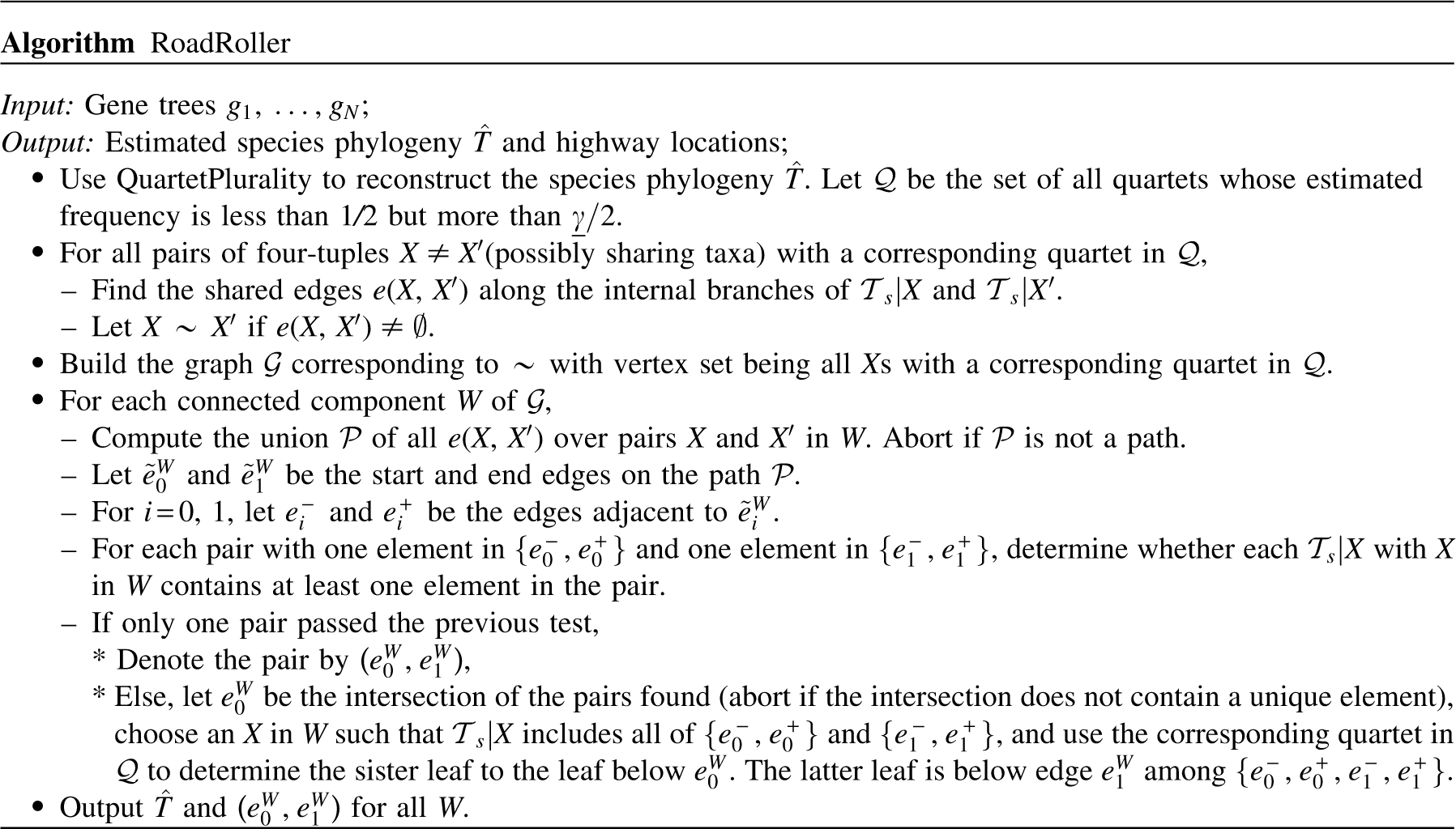
Algorithm RoadRoller.

Theorem 6 (Inferring highways)

Consider the Bounded-rates model with R=+∞and assume that B < +∞is constant. Assume further that there are constants \documentclass{aastex}\usepackage{amsbsy}\usepackage{amsfonts}\usepackage{amssymb}\usepackage{bm}\usepackage{mathrsfs}\usepackage{pifont}\usepackage{stmaryrd}\usepackage{textcomp}\usepackage{portland, xspace}\usepackage{amsmath, amsxtra}\pagestyle{empty}\DeclareMathSizes{10}{9}{7}{6}\begin{document} $$0 < \underline \gamma < \overline \gamma < + \infty$$ \end{document} such that \documentclass{aastex}\usepackage{amsbsy}\usepackage{amsfonts}\usepackage{amssymb}\usepackage{bm}\usepackage{mathrsfs}\usepackage{pifont}\usepackage{stmaryrd}\usepackage{textcomp}\usepackage{portland, xspace}\usepackage{amsmath, amsxtra}\pagestyle{empty}\DeclareMathSizes{10}{9}{7}{6}\begin{document} \begin{align*}\underline \gamma < \gamma_{ \beta} < \overline \gamma , \quad \beta = 1 , \ldots , B.\end{align*} \end{document}

and Assumption 1 holds then it is possible to reconstruct the topology of the extant phylogeny as well as the highway edges w.h.p. from N=Ω(log n⁺) gene tree topologies if \documentclass{aastex}\usepackage{amsbsy}\usepackage{amsfonts}\usepackage{amssymb}\usepackage{bm}\usepackage{mathrsfs}\usepackage{pifont}\usepackage{stmaryrd}\usepackage{textcomp}\usepackage{portland, xspace}\usepackage{amsmath, amsxtra}\pagestyle{empty}\DeclareMathSizes{10}{9}{7}{6}\begin{document} $$\overline \lambda$$ \end{document} is such that \documentclass{aastex}\usepackage{amsbsy}\usepackage{amsfonts}\usepackage{amssymb}\usepackage{bm}\usepackage{mathrsfs}\usepackage{pifont}\usepackage{stmaryrd}\usepackage{textcomp}\usepackage{portland, xspace}\usepackage{amsmath, amsxtra}\pagestyle{empty}\DeclareMathSizes{10}{9}{7}{6}\begin{document} \begin{align*}\bold \Lambda = O \left( { \frac { n^ { + } } { \log n^ { + } } } \right).\end{align*} \end{document}

Proof (Theorem 6)

Consider a four-tuple X such that \documentclass{aastex}\usepackage{amsbsy}\usepackage{amsfonts}\usepackage{amssymb}\usepackage{bm}\usepackage{mathrsfs}\usepackage{pifont}\usepackage{stmaryrd}\usepackage{textcomp}\usepackage{portland, xspace}\usepackage{amsmath, amsxtra}\pagestyle{empty}\DeclareMathSizes{10}{9}{7}{6}\begin{document} $${ \cal T} _s \mid X$$ \end{document} contains at least one highway location and such that the quartet \documentclass{aastex}\usepackage{amsbsy}\usepackage{amsfonts}\usepackage{amssymb}\usepackage{bm}\usepackage{mathrsfs}\usepackage{pifont}\usepackage{stmaryrd}\usepackage{textcomp}\usepackage{portland, xspace}\usepackage{amsmath, amsxtra}\pagestyle{empty}\DeclareMathSizes{10}{9}{7}{6}\begin{document} $$q_s^X$$ \end{document} is modified by the corresponding highway. Because such a highway must connect a leg of \documentclass{aastex}\usepackage{amsbsy}\usepackage{amsfonts}\usepackage{amssymb}\usepackage{bm}\usepackage{mathrsfs}\usepackage{pifont}\usepackage{stmaryrd}\usepackage{textcomp}\usepackage{portland, xspace}\usepackage{amsmath, amsxtra}\pagestyle{empty}\DeclareMathSizes{10}{9}{7}{6}\begin{document} $${ \cal T} _s \mid X$$ \end{document} to a subtree on the other side of the internal branch of \documentclass{aastex}\usepackage{amsbsy}\usepackage{amsfonts}\usepackage{amssymb}\usepackage{bm}\usepackage{mathrsfs}\usepackage{pifont}\usepackage{stmaryrd}\usepackage{textcomp}\usepackage{portland, xspace}\usepackage{amsmath, amsxtra}\pagestyle{empty}\DeclareMathSizes{10}{9}{7}{6}\begin{document} $${ \cal T} _s \mid X$$ \end{document} , our galled tree assumption implies that any given quartet tree can be affected by at most one highway, otherwise the corresponding cycles would intersect along the internal branch. Hence, from the proof of Theorem 5 and the assumption that \documentclass{aastex}\usepackage{amsbsy}\usepackage{amsfonts}\usepackage{amssymb}\usepackage{bm}\usepackage{mathrsfs}\usepackage{pifont}\usepackage{stmaryrd}\usepackage{textcomp}\usepackage{portland, xspace}\usepackage{amsmath, amsxtra}\pagestyle{empty}\DeclareMathSizes{10}{9}{7}{6}\begin{document} $$ {\overline \gamma} < \frac { 1 } { 2 } $$ \end{document} (instead of \documentclass{aastex}\usepackage{amsbsy}\usepackage{amsfonts}\usepackage{amssymb}\usepackage{bm}\usepackage{mathrsfs}\usepackage{pifont}\usepackage{stmaryrd}\usepackage{textcomp}\usepackage{portland, xspace}\usepackage{amsmath, amsxtra}\pagestyle{empty}\DeclareMathSizes{10}{9}{7}{6}\begin{document} $$ {\overline \gamma} < \frac { 1 } { 2B } $$ \end{document} ), we can reconstruct the extant phylogeny.

Further, it follows by the proof of Theorem 5 that, if \documentclass{aastex}\usepackage{amsbsy}\usepackage{amsfonts}\usepackage{amssymb}\usepackage{bm}\usepackage{mathrsfs}\usepackage{pifont}\usepackage{stmaryrd}\usepackage{textcomp}\usepackage{portland, xspace}\usepackage{amsmath, amsxtra}\pagestyle{empty}\DeclareMathSizes{10}{9}{7}{6}\begin{document} $$\underline \gamma > 0$$ \end{document} and C₁ is small enough, the second most frequent quartet over a four-tuple as above is the one obtained by going through the highway. Let \documentclass{aastex}\usepackage{amsbsy}\usepackage{amsfonts}\usepackage{amssymb}\usepackage{bm}\usepackage{mathrsfs}\usepackage{pifont}\usepackage{stmaryrd}\usepackage{textcomp}\usepackage{portland, xspace}\usepackage{amsmath, amsxtra}\pagestyle{empty}\DeclareMathSizes{10}{9}{7}{6}\begin{document} $${ \cal Q}$$ \end{document} be the set of all quartets whose estimated frequency is less than 1/2 but more than \documentclass{aastex}\usepackage{amsbsy}\usepackage{amsfonts}\usepackage{amssymb}\usepackage{bm}\usepackage{mathrsfs}\usepackage{pifont}\usepackage{stmaryrd}\usepackage{textcomp}\usepackage{portland, xspace}\usepackage{amsmath, amsxtra}\pagestyle{empty}\DeclareMathSizes{10}{9}{7}{6}\begin{document} $$\underline \gamma / 2$$ \end{document} . By the previous argument and Lemma 3 (see the proof of Theorem 1 for a similar computation), \documentclass{aastex}\usepackage{amsbsy}\usepackage{amsfonts}\usepackage{amssymb}\usepackage{bm}\usepackage{mathrsfs}\usepackage{pifont}\usepackage{stmaryrd}\usepackage{textcomp}\usepackage{portland, xspace}\usepackage{amsmath, amsxtra}\pagestyle{empty}\DeclareMathSizes{10}{9}{7}{6}\begin{document} $${ \cal Q}$$ \end{document} contains w.h.p. exactly those quartets affected by a highway.

For X, X′ with quartets in \documentclass{aastex}\usepackage{amsbsy}\usepackage{amsfonts}\usepackage{amssymb}\usepackage{bm}\usepackage{mathrsfs}\usepackage{pifont}\usepackage{stmaryrd}\usepackage{textcomp}\usepackage{portland, xspace}\usepackage{amsmath, amsxtra}\pagestyle{empty}\DeclareMathSizes{10}{9}{7}{6}\begin{document} $${ \cal Q}$$ \end{document} , write X ∼ X′ if the quartet trees \documentclass{aastex}\usepackage{amsbsy}\usepackage{amsfonts}\usepackage{amssymb}\usepackage{bm}\usepackage{mathrsfs}\usepackage{pifont}\usepackage{stmaryrd}\usepackage{textcomp}\usepackage{portland, xspace}\usepackage{amsmath, amsxtra}\pagestyle{empty}\DeclareMathSizes{10}{9}{7}{6}\begin{document} $${ \cal T} _s \mid X$$ \end{document} and \documentclass{aastex}\usepackage{amsbsy}\usepackage{amsfonts}\usepackage{amssymb}\usepackage{bm}\usepackage{mathrsfs}\usepackage{pifont}\usepackage{stmaryrd}\usepackage{textcomp}\usepackage{portland, xspace}\usepackage{amsmath, amsxtra}\pagestyle{empty}\DeclareMathSizes{10}{9}{7}{6}\begin{document} $${ \cal T} _s \mid X^{ \prime}$$ \end{document} share an edge along their internal branch. Let e(X, X′) be the set of all such shared edges. Note that, although we are considering four-tuples affected by highways, we are working on the species phylogeny \documentclass{aastex}\usepackage{amsbsy}\usepackage{amsfonts}\usepackage{amssymb}\usepackage{bm}\usepackage{mathrsfs}\usepackage{pifont}\usepackage{stmaryrd}\usepackage{textcomp}\usepackage{portland, xspace}\usepackage{amsmath, amsxtra}\pagestyle{empty}\DeclareMathSizes{10}{9}{7}{6}\begin{document} $${ \cal T} _s$$ \end{document} which has been reconstructed.

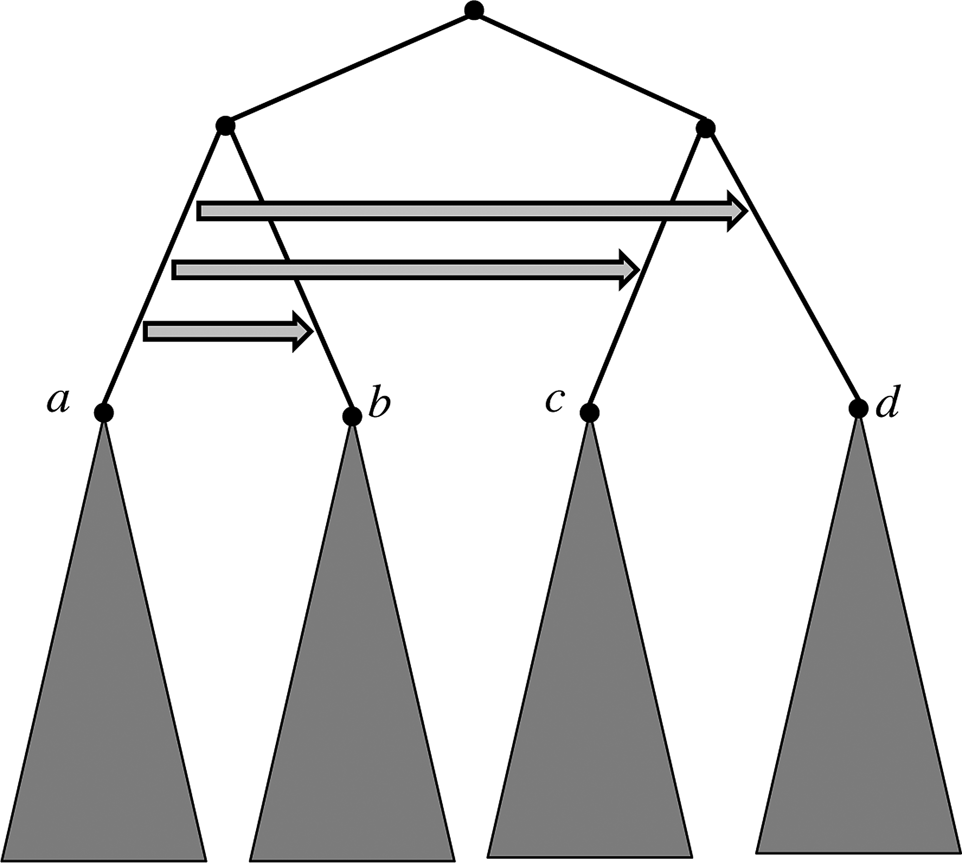
By the argument above, quartets sharing an edge along their internal branch are necessarily affected by the same highway. Take the transitive closure ∼_* of ∼. Let W be an equivalence class of ∼_*. We reconstruct the corresponding highway as follows. The union of all edges in e(X, X′) for some pair X, X′ in W forms a path \documentclass{aastex}\usepackage{amsbsy}\usepackage{amsfonts}\usepackage{amssymb}\usepackage{bm}\usepackage{mathrsfs}\usepackage{pifont}\usepackage{stmaryrd}\usepackage{textcomp}\usepackage{portland, xspace}\usepackage{amsmath, amsxtra}\pagestyle{empty}\DeclareMathSizes{10}{9}{7}{6}\begin{document} $${ \cal P}$$ \end{document} in \documentclass{aastex}\usepackage{amsbsy}\usepackage{amsfonts}\usepackage{amssymb}\usepackage{bm}\usepackage{mathrsfs}\usepackage{pifont}\usepackage{stmaryrd}\usepackage{textcomp}\usepackage{portland, xspace}\usepackage{amsmath, amsxtra}\pagestyle{empty}\DeclareMathSizes{10}{9}{7}{6}\begin{document} $${ \cal T} _s$$ \end{document} . Let \documentclass{aastex}\usepackage{amsbsy}\usepackage{amsfonts}\usepackage{amssymb}\usepackage{bm}\usepackage{mathrsfs}\usepackage{pifont}\usepackage{stmaryrd}\usepackage{textcomp}\usepackage{portland, xspace}\usepackage{amsmath, amsxtra}\pagestyle{empty}\DeclareMathSizes{10}{9}{7}{6}\begin{document} $$\tilde{e}_0^{W}$$ \end{document} and \documentclass{aastex}\usepackage{amsbsy}\usepackage{amsfonts}\usepackage{amssymb}\usepackage{bm}\usepackage{mathrsfs}\usepackage{pifont}\usepackage{stmaryrd}\usepackage{textcomp}\usepackage{portland, xspace}\usepackage{amsmath, amsxtra}\pagestyle{empty}\DeclareMathSizes{10}{9}{7}{6}\begin{document} $$\tilde{e}_1^{W}$$ \end{document} be the start and end edges on this path. The highway corresponding to W connects an edge \documentclass{aastex}\usepackage{amsbsy}\usepackage{amsfonts}\usepackage{amssymb}\usepackage{bm}\usepackage{mathrsfs}\usepackage{pifont}\usepackage{stmaryrd}\usepackage{textcomp}\usepackage{portland, xspace}\usepackage{amsmath, amsxtra}\pagestyle{empty}\DeclareMathSizes{10}{9}{7}{6}\begin{document} $$e_0^W$$ \end{document} adjacent to \documentclass{aastex}\usepackage{amsbsy}\usepackage{amsfonts}\usepackage{amssymb}\usepackage{bm}\usepackage{mathrsfs}\usepackage{pifont}\usepackage{stmaryrd}\usepackage{textcomp}\usepackage{portland, xspace}\usepackage{amsmath, amsxtra}\pagestyle{empty}\DeclareMathSizes{10}{9}{7}{6}\begin{document} $$\tilde{e}_0^{W}$$ \end{document} with an edge \documentclass{aastex}\usepackage{amsbsy}\usepackage{amsfonts}\usepackage{amssymb}\usepackage{bm}\usepackage{mathrsfs}\usepackage{pifont}\usepackage{stmaryrd}\usepackage{textcomp}\usepackage{portland, xspace}\usepackage{amsmath, amsxtra}\pagestyle{empty}\DeclareMathSizes{10}{9}{7}{6}\begin{document} $$e_1^W$$ \end{document} adjacent to \documentclass{aastex}\usepackage{amsbsy}\usepackage{amsfonts}\usepackage{amssymb}\usepackage{bm}\usepackage{mathrsfs}\usepackage{pifont}\usepackage{stmaryrd}\usepackage{textcomp}\usepackage{portland, xspace}\usepackage{amsmath, amsxtra}\pagestyle{empty}\DeclareMathSizes{10}{9}{7}{6}\begin{document} $$\tilde{e}_1^{W}$$ \end{document} (see Fig. 5). (Note that a highway is represented by exactly one W because w.h.p. all quartets affected by this highway are in \documentclass{aastex}\usepackage{amsbsy}\usepackage{amsfonts}\usepackage{amssymb}\usepackage{bm}\usepackage{mathrsfs}\usepackage{pifont}\usepackage{stmaryrd}\usepackage{textcomp}\usepackage{portland, xspace}\usepackage{amsmath, amsxtra}\pagestyle{empty}\DeclareMathSizes{10}{9}{7}{6}\begin{document} $${ \cal Q}$$ \end{document} and they are all connected under ∼; see Fig. 5.)

FIG. 5.

Setup in the proof of Theorem 6. The gray arrow indicates a highway. Here \documentclass{aastex}\usepackage{amsbsy}\usepackage{amsfonts}\usepackage{amssymb}\usepackage{bm}\usepackage{mathrsfs}\usepackage{pifont}\usepackage{stmaryrd}\usepackage{textcomp}\usepackage{portland, xspace}\usepackage{amsmath, amsxtra}\pagestyle{empty}\DeclareMathSizes{10}{9}{7}{6}\begin{document} $$X = \{ a , b , c , d \} , { \cal T}_s \mid X = ab \mid cd$$ \end{document} and \documentclass{aastex}\usepackage{amsbsy}\usepackage{amsfonts}\usepackage{amssymb}\usepackage{bm}\usepackage{mathrsfs}\usepackage{pifont}\usepackage{stmaryrd}\usepackage{textcomp}\usepackage{portland, xspace}\usepackage{amsmath, amsxtra}\pagestyle{empty}\DeclareMathSizes{10}{9}{7}{6}\begin{document} $$bc \mid ad \in { \cal Q}$$ \end{document} .

As we argued in the proof of Lemma 1, all quartets affected by the highway corresponding to W contain at least one leaf in a pruned subtree. Because we allow LGT events in both directions along a highway, there are two potential pruned subtrees. Moreover, the other three leaves must be in separate subtrees hanging from the path \documentclass{aastex}\usepackage{amsbsy}\usepackage{amsfonts}\usepackage{amssymb}\usepackage{bm}\usepackage{mathrsfs}\usepackage{pifont}\usepackage{stmaryrd}\usepackage{textcomp}\usepackage{portland, xspace}\usepackage{amsmath, amsxtra}\pagestyle{empty}\DeclareMathSizes{10}{9}{7}{6}\begin{document} $${ \cal P}$$ \end{document} . By our assumption, there are at least three such subtrees (in addition to the two potentially pruned subtrees).

Hence, the pruned subtrees can be identified by checking the four-tuples in W and finding the pairs of subtrees with at least one of them present in all of W. If there is a unique such pair, this gives the two highway edges and we are done. Otherwise, the recipient edge is the intersection of the pairs found. To identify the donor edge, one simply needs to use a four-tuple X of leaves in the four adjacent subtrees to the endpoints of \documentclass{aastex}\usepackage{amsbsy}\usepackage{amsfonts}\usepackage{amssymb}\usepackage{bm}\usepackage{mathrsfs}\usepackage{pifont}\usepackage{stmaryrd}\usepackage{textcomp}\usepackage{portland, xspace}\usepackage{amsmath, amsxtra}\pagestyle{empty}\DeclareMathSizes{10}{9}{7}{6}\begin{document} $${ \cal P}$$ \end{document} and check to which branch of \documentclass{aastex}\usepackage{amsbsy}\usepackage{amsfonts}\usepackage{amssymb}\usepackage{bm}\usepackage{mathrsfs}\usepackage{pifont}\usepackage{stmaryrd}\usepackage{textcomp}\usepackage{portland, xspace}\usepackage{amsmath, amsxtra}\pagestyle{empty}\DeclareMathSizes{10}{9}{7}{6}\begin{document} $${ \cal T} _s \mid X$$ \end{document} the subtree corresponding to the recipient edge is moved in \documentclass{aastex}\usepackage{amsbsy}\usepackage{amsfonts}\usepackage{amssymb}\usepackage{bm}\usepackage{mathrsfs}\usepackage{pifont}\usepackage{stmaryrd}\usepackage{textcomp}\usepackage{portland, xspace}\usepackage{amsmath, amsxtra}\pagestyle{empty}\DeclareMathSizes{10}{9}{7}{6}\begin{document} $${ \cal Q}$$ \end{document} (that is, in the highway-affected quartet topology). ■

5. Distance Method and Sequence Lengths

In this section, in the highway-free case, we analyze an alternative, distance-based approach that has been considered in the literature, and we provide sequence-length requirements. Although the quartet-based method analyzed in Section 3 can in principle handle arbitrary branch lengths (as only the topology of the gene trees is used), here we need to assume that the gene-tree branch lengths are determined by interspeciation times and lineage-specific rates of substitution. For simplicity, we assume that there is no gene-specific substitution rate. In practice, one could incorporate such rates by using a normalization procedure as detailed in Kim and Salisbury (2001) and Ge et al. (2005).

5.1. A distance-based approach

We analyze a distance-based approach similar to that introduced in Kim and Salisbury (2001) and studied empirically in Ge et al. (2005). Given branch lengths, a gene tree is naturally equipped with a tree metric on the leaves D_g : L_g × L_g → (0, +∞) defined as follows \documentclass{aastex}\usepackage{amsbsy}\usepackage{amsfonts}\usepackage{amssymb}\usepackage{bm}\usepackage{mathrsfs}\usepackage{pifont}\usepackage{stmaryrd}\usepackage{textcomp}\usepackage{portland, xspace}\usepackage{amsmath, amsxtra}\pagestyle{empty}\DeclareMathSizes{10}{9}{7}{6}\begin{document} \begin{align*}\forall u , v \in L_g , \ { \rm D}_g ( u , v ) = \sum_{e \in { \rm P}_g ( u , v ) } \omega_g ( e ) ,\end{align*} \end{document}

where P_g(u, v) is the set of edges on the path between u and v in T_g. We will refer to D_g(u, v) as the evolutionary distance between u and v under g.

For each pair of extant species {a, b}, we compute the median \documentclass{aastex}\usepackage{amsbsy}\usepackage{amsfonts}\usepackage{amssymb}\usepackage{bm}\usepackage{mathrsfs}\usepackage{pifont}\usepackage{stmaryrd}\usepackage{textcomp}\usepackage{portland, xspace}\usepackage{amsmath, amsxtra}\pagestyle{empty}\DeclareMathSizes{10}{9}{7}{6}\begin{document} \begin{align*}{ \rm D_m} ( a , b ) = { \rm Median} \{ { \rm D}_{g_i} ( a , b ) : i = 1 , \ldots , N , \ \{ a , b \} \subseteq L_{g_i} \} .\end{align*} \end{document}

We abort if a pair is not included in any of the gene trees. We then use the distance matrix D_m to build a tree using the Short Quartet Method (Erdös et al., 1999a) (or any other statistically consistent, fast-converging distance-based method). We will refer to this method as the MedianTree (MT) method. The algorithm is detailed in Figure 6.

FIG. 6.

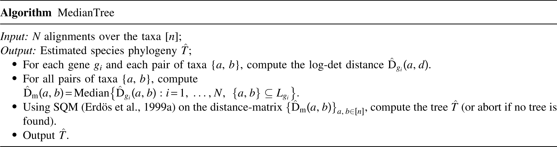
Algorithm MedianTree.

Probabilistic analysis

Define the maximum path weight (MPW) \documentclass{aastex}\usepackage{amsbsy}\usepackage{amsfonts}\usepackage{amssymb}\usepackage{bm}\usepackage{mathrsfs}\usepackage{pifont}\usepackage{stmaryrd}\usepackage{textcomp}\usepackage{portland, xspace}\usepackage{amsmath, amsxtra}\pagestyle{empty}\DeclareMathSizes{10}{9}{7}{6}\begin{document} \begin{align*}\Upsilon^{\; ( 2 ) } = \max \{ \bold \Lambda_X : X \subseteq ( L_s^ + ) ^2 \} .\end{align*} \end{document}

Then:

Lemma 5 (Probability of a miss: Distance case)

Let T_g=(V_g, E_g, L_g; ω_g) be a gene tree distributed according to the random LGT model such that X={a, b} ⊆ L_g. Let D_s(a, b) be the evolutionary distance between a and b under the topology of the extant phylogeny (that is, under the event that no LGT has occurred). Then \documentclass{aastex}\usepackage{amsbsy}\usepackage{amsfonts}\usepackage{amssymb}\usepackage{bm}\usepackage{mathrsfs}\usepackage{pifont}\usepackage{stmaryrd}\usepackage{textcomp}\usepackage{portland, xspace}\usepackage{amsmath, amsxtra}\pagestyle{empty}\DeclareMathSizes{10}{9}{7}{6}\begin{document} \begin{align*}{\mathbb P} [ { \rm D}_g ( a , b ) = { \rm D}_s ( a , b ) \mid X \subseteq L_g ] \geq \exp \left( - \Upsilon^{\; ( 2 ) } \right) .\end{align*} \end{document}

Proof (Lemma 5)

The proof is similar to that of Lemma 1. ■

Lemma 6 (Bound on path weight: Bounded-rates case)

Under the bounded-rates model, it holds that \documentclass{aastex}\usepackage{amsbsy}\usepackage{amsfonts}\usepackage{amssymb}\usepackage{bm}\usepackage{mathrsfs}\usepackage{pifont}\usepackage{stmaryrd}\usepackage{textcomp}\usepackage{portland, xspace}\usepackage{amsmath, amsxtra}\pagestyle{empty}\DeclareMathSizes{10}{9}{7}{6}\begin{document} \begin{align*}\Upsilon^{\; ( 2 ) } = O \left( \overline \lambda \log n^ {+} \right) .\end{align*} \end{document} ■

Proof (Lemma 6)

Note that \documentclass{aastex}\usepackage{amsbsy}\usepackage{amsfonts}\usepackage{amssymb}\usepackage{bm}\usepackage{mathrsfs}\usepackage{pifont}\usepackage{stmaryrd}\usepackage{textcomp}\usepackage{portland, xspace}\usepackage{amsmath, amsxtra}\pagestyle{empty}\DeclareMathSizes{10}{9}{7}{6}\begin{document} \begin{align*} \max \{ {\bold \Lambda}_X : X \subseteq ( L_s^ { + } ) ^2 \} \leq 2 {\overline {\lambda }} { \overline { \tau }} { \frac {\overline{ \tau }} { \underline {\tau } }} \log_2 n^ { + } .\end{align*} \end{document}

Lemma 7 (Bound on path weight: Yule case)

Under the Yule model, it holds that \documentclass{aastex}\usepackage{amsbsy}\usepackage{amsfonts}\usepackage{amssymb}\usepackage{bm}\usepackage{mathrsfs}\usepackage{pifont}\usepackage{stmaryrd}\usepackage{textcomp}\usepackage{portland, xspace}\usepackage{amsmath, amsxtra}\pagestyle{empty}\DeclareMathSizes{10}{9}{7}{6}\begin{document} \begin{align*}\Upsilon^{ ( 2 ) } = \Theta \left( \overline \lambda \log n \right) ,\end{align*} \end{document}

with probability approaching 1 as n → +∞.

Proof (Lemma 7)

The proof is similar to that of Lemma 4. ■

Proof (Theorems 1 and 3)

Using MT and Lemmas 6 and 7, the proof of Theorem 1 (and of Theorem 3) follows from the same lines as that of Theorem 1. Note however that our extra assumption on the gene-tree branch lengths is needed here to ensure that evolutionary distances are the same across all genes. ■

5.2. Taking into account sequence length

We have assumed so far that gene tree topologies and evolutionary distances are known perfectly. Of course, this is not the case in practice, and the effect of sequence length must be accounted for. One issue that arises is that LGT events may create very short branches that are difficult to infer. Nevertheless, we can prove the following. We assume that sequence data is generated independently on each gene tree according to a GTR model. Evolutionary distances are estimated using the log-det distance. See, for example, Semple and Steel (2003) for background on GTR models of substitution and the log-det distance. We assume n⁻=0 for simplicity.

Theorem 7 (Sequence-length requirements)

Under the bounded-rates and Yule models for the species phylogeny and the GTR model for sequences, assuming that substitution rates are bounded between constants, a sequence length per gene polynomial in n suffices for the MT algorithm to succeed if the number of genes is at most polynomial in n.

Proof (Theorem 7)

We only discuss the Yule model. The argument for the bounded-rates model is similar.

In our second proof of Theorem 3, we relied on the fact that, for every pair of taxa w.h.p., a strict majority of the gene-tree evolutionary distances has not been affected by LGT. Hence, if the worst case estimation error on the evolutionary distances is ɛ, then the median of the estimated distances must be in the interval [D_s(a, b) − ɛ, D_s(a, b) + ɛ] for all pairs of taxa a, b. Further, by the concentration bounds in Erdös et al. (1999b), for the SQM step of our MT algorithm to return the correct topology w.h.p., the sequence length must scale as an exponential of the depth of the tree divided by the square of the shortest branch length.

Under the Yule model, with probability approaching 1, the depth of the tree is O(log n) (by the proof of Lemma 4) and the shortest branch length (the minimum of O(n) exponentials with mean O(1)) is 1/poly(n). Hence the result follows.² ■

6. Discussion

We have shown that a species phylogeny or network can be reconstructed despite high levels of random LGT, and we have provided explicit quantitative bounds on tolerable rates of LGT. Moreover, our analysis sheds light on effective approaches for species tree building in the presence of LGT. Several problems remain open:

• Galtier and Daubin (2008) hypothesize that random LGT only becomes a significant hurdle when the rate of LGT greatly exceeds the rate of diversification. In our setting, this would imply that a value of Λ as high as Ω(n) may be achievable. Note that branches close to the leaves are particularly easy to reconstruct because they lie on small quartet trees that are less likely than deep ones to be hit by an LGT event. Is a recursive approach starting from the leaves possible here? See Mossel (2004) and Daskalakis et al. (2011) for recursive approaches in a related context.

• In a related problem, we have analyzed distance-based and quartet-based methods. A better understanding of bipartition-based approaches is needed and may lead to a higher threshold for Λ.

• What can be proved when a model of extinction is incorporated?

• What can be proved when the number of genes is significantly less than log n?

• In the presence of highways, dealing with more general network settings would be desirable. Also, our definition of highways as connecting two edges is somewhat restrictive. In general, one is also interested in preferential genetic transfers between clades.

• On the practical side, the predictions made here should be further tested on real and simulated datasets. We note that there is extisting work in this direction (Beiko et al., 2005; Ge et al., 2005; Galtier, 2007; Puigbo et al., 2009, 2010; Koonin et al., 2011; Bansal et al., 2011).

Footnotes

Acknowledgments

S.R. was supported by NSF grant DMS-1007144. S.S. was supported by the USA-Israel Binational Science Foundation and by the Israel Science Foundation.

Disclosure Statement

No competing financial interests exist.

1

Note that such estimates are typically based on small numbers of genomes, and, therefore, are probably lower than reality (Galtier and Daubin, ).

2

Note that unlike Erdös et al. (), we use the interspeciation times generated by the continuous-time branching process. In particular, their “few logs” result does not apply to our setting.

References

Arvestad

, Lagergren

, Sennblad

2009. The gene evolution model and computing its associated probabilities. J. ACM, 56,2Article 7.

Athreya

K.B.

, Ney

P.E.

1972. Branching processes. Springer-Verlag: New YorkDie Grundlehren der mathematischen Wissenschaften, Band 196.

Bandelt

H.-J.

, Dress

1986. Reconstructing the shape of a tree from observed dissimilarity data. Adv. Appl. Math., 7:309–343.

Bansal

M.S.

, Banay

, Gogarten

J.P.

et al. 2011. Detecting highways of horizontal gene transfer. J. Comput. Biol., 18:1087–1114.

Bapteste

, Susko

, Leigh

et al. 2005. Do orthologous gene phylogenies really support tree-thinking? BMC Evol. Biol., 5:33.

Baum

1992. Combining trees as a way of combining data sets for phylogenetic inference. Taxon, 41:3–10.

Beiko

, Harlow

, Ragan

2005. Highways of gene sharing in prokaryotes. Proc. Natl. Acad. Sci. USA, 102:14332–14337.

Berry

, Gascuel

2001. Inferring evolutionary trees with strong combinatorial evidence. Theor. Comput. Sci., 240:271–298.

Buneman

1971. The recovery of trees from measures of dissimilarity, 387–395. Hodson

, Kendall

, Tautu

Anglo-Romanian Conference on Mathematics in the Archaeological and Historical Sciences. Edinburgh University Press: Mamaia, Romania.

10.

Chung

, Ane

2011. Comparing two bayesian methods for gene tree/species tree reconstruction: Simulations with incomplete lineage sorting and horizontal gene transfer. Syst. Biol., 60:261–275.

11.

Csürös

, Miklós

2006. A probabilistic model for gene content evolution with duplication, loss, and horizontal transfer. RECOMB, 206–220.

12.

Dagan

, Martin

2006. The tree of one percent. Genome Biol., 7:118.

13.

Daskalakis

, Roch

2010. Alignment-free phylogenetic reconstruction. RECOMB, 123–137.

14.

Daskalakis

, Mossel

, Roch

2011. Evolutionary trees and the ising model on the bethe lattice: a proof of steel's conjecture. Probab. Theory Rel., 149:149–189.

15.

Degnan

J.H.

, Rosenberg

N.A.

2009. Gene tree discordance, phylogenetic inference and the multispecies coalescent. Trends Ecol. Evol., 24:332–340.

16.

Delsuc

, Brinkmann

, Philippe

2005. Phylogenomics and the reconstruction of the tree of life. Nat. Rev. Genet., 6:361–375.

17.

Dewhirst

F.E.

, Shen

, Scimeca

et al. 2005. Discordant 16S and 23S rRNA gene phylogenies for the Genus Helicobacter: Implications for phylogenetic inference and systematics. J. Bacteriol., 187:6106–6118.

18.

Doolittle

, Bapteste

2007. Pattern pluralism and the tree of life hypothesis. Proc. Natl. Acad. Sci. USA, 104:2043–2049.

19.

Eisen

J.A.

, Fraser

C.M.

2003. Phylogenomics: Intersection of evolution and genomics. Science, 300:1706–1707.

20.

Erdös

P.L.

, Steel

M.A.

, Székely

L.A.

et al. 1999a. A few logs suffice to build (almost) all trees (part 1) Random Struct. Algor., 14:153–184.

21.

Erdös

P.L.

, Steel

M.A.

, Székely

L.A.

et al. 1999b. A few logs suffice to build (almost) all trees (part 2) Theor. Comput. Sci., 221:77–118.

22.

Galtier

2007. A model of horizontal gene transfer and the bacterial phylogeny problem. Syst. Biol., 56:633–642.

23.

Galtier

, Daubin

2008. Dealing with incongruence in phylogenomic analyses. Philos. Trans. R. Soc. Lond. B Biol. Sci., 363:4023–4029.

24.

, Wang

, Kim

2005. The cobweb of life revealed by genome-scale estimates of horizontal gene transfer. PLoS Biol., 3:e316.

25.

Gogarten

J.P.

, Doolittle

W.F.

, Lawrence

J.G.

2002. Prokaryotic evolution in light of gene transfer. Mol. Biol. Evol., 19:2226–2238.

26.

Gogarten

J.P.

, Townsend

J.P.

2005. Horizontal gene transfer, genome innovation and evolution. Nat. Rev. Micro., 3:679–687.

27.

Huson

D.H.

, Rupp

, Scornavacca

2010. Phylogenetic Networks: Concepts, Algorithms and Applications. Cambridge University Press: Cambridge.

28.

Jin

, Nakhleh

, Snir

et al. 2006. Maximum likelihood of phylogenetic networks. Bioinformatics, 22:2604–11.

29.

Jin

, Nakhleh

, Snir

et al. 2009. Parsimony score of phylogenetic networks: Hardness results and a linear-time heuristic. IEEE/ACM Trans. Comput. Biology Bioinform., 6:495–505.

30.

Joly

, McLenachan

P.A.

, Lockhart

P.J.

2009. A statistical approach for distinguishing hybridization and incomplete lineage sorting. Am. Nat., 174:E54–E70.

31.

Kim

, Salisbury

B.A.

2001. A tree obscured by vines: Horizontal gene transfer and the median tree method of estimating species phylogeny. Pacific Symposium on Biocomputing, 571–582.

32.

Koonin

2007. The biological big bang model for the major transitions in evolution. Biol. Direct, 2:21.

33.

Koonin

E.V.

, Puigbo

, Wolf

Y.I.

2011. Comparison of phylogenetic trees and search for a central trend in the forest of life. J. Comput. Biol., 18:917–924.

34.

Kubatko

L.S.

2009. Identifying hybridization events in the presence of coalescence via model selection. Syst. Biol., 58:478–488.

35.

Lindvall

1992. Lectures on the Coupling Method. Wiley: New York.

36.

Maddison

W.P.

1997. Gene trees in species trees. Syst. Biol., 46:523–536.

37.

Meng

, Kubatko

L.S.

2009. Detecting hybrid speciation in the presence of incomplete lineage sorting using gene tree incongruence: A model. Theor. Popul. Biol., 75:35–45.

38.

Mossel

2004. Phase transitions in phylogeny. Trans. Amer. Math. Soc., 356:2379–2404.

39.

Motwani

, Raghavan

1995. Randomized algorithms. Cambridge University Press: Cambridge.

40.

Puigbo

, Wolf

, Koonin

2009. Search for a ‘tree of life’ in the thicket of the phylogenetic forest. J. Biol., 8:59.

41.

Puigbo

, Wolf

Y.I.

, Koonin

E.V.

2010. The tree and net components of prokaryote evolution. Genome Biol. Evol., 2:745–756.

42.

Ragan

1992. Matrix representation in reconstructing phylogenetic-relationships among the eukaryotes. Biosystems, 28:47–55.

43.

Ragan

M.A.

, Beiko

R.G.

2009. Lateral genetic transfer: open issues. Philos. Trans. R. Soc. Lond. B Biol. Sci., 364:2241–2251.

44.

Rannala

, Yang

1996. Probability distribution of molecular evolutionary trees: A new method of phylogenetic inference. J. Mol. Evol., 43:304–311.

45.

Roch

, Snir

2012. Recovering the tree-like trend of evolution despite extensive lateral genetic transfer: A probabilistic analysis. RECOMB, 224–238.

46.

Schouls

L.M.

, Schot

C.S.

, Jacobs

J.A.

2003. Horizontal transfer of segments of the 16S rRNA genes between species of the Streptococcus anginosus group. J. Bacteriol., 185:7241–7246.

47.

Semple

, Steel

2003. Phylogenetics. 22 Mathematics and its Applications series. Oxford University Press: New York.

48.

Smets

B.F.

, Barkay

2005. Horizontal gene transfer: perspectives at a crossroads of scientific disciplines. Nat. Rev. Micro., 3:675–678.

49.

Snir

, Rao

2010. Quartets maxcut: A divide and conquer quartets algorithm. IEEE/ACM Trans. Comput. Biology Bioinform., 7:704–718.

50.

Snir

, Rao

2012. Quartet maxcut: A fast algorithm for amalgamating quartet trees. Mol. Phylogenet. Evol., 62:1–8.

51.

Steel

1992. The complexity of reconstructing trees from qualitative characters and subtress. J. Classif., 9:91–116.

52.

Suchard

M.A.

2005. Stochastic models for horizontal gene transfer. Genetics, 170:419–431.

53.

Than

, Ruths

, Innan

et al. 2007. Confounding factors in hgt detection: Statistical error, coalescent effects, and multiple solutions. J. Comput. Biol., 14:517–535.

54.

van Berkum

, Terefework

, Paulin

et al. 2003. Discordant phylogenies within the rrn loci of rhizobia. J. Bacteriol., 185:2988–2998.

55.

Yap

W.H.

, Zhang

, Wang

1999. Distinct types of rrna operons exist in the genome of the Actinomycete Thermomonospora chromogena and evidence for horizontal transfer of an entire rRNA operon. J. Bacteriol., 181:5201–5209.

56.

, Than

, Degnan

J.H.

et al. 2011. Coalescent histories on phylogenetic networks and detection of hybridization despite incomplete lineage sorting. Syst. Biol., 60:138–149.

57.

Zhaxybayeva

, Gogarten

J.P.

, Charlebois

R.L.

et al. 2006. Phylogenetic analyses of cyanobacterial genomes: Quantification of horizontal gene transfer events. Genome Res., 16:1099–1108.

58.

Zhaxybayeva

, Lapierre

, Gogarten

2004. Genome mosaicism and organismal lineages. Trends Genet., 20:254–260.