Ballast : A Ball-based Algorithm for Structural Motifs

Abstract

Structural motifs encapsulate local sequence-structure-function relationships characteristic of related proteins, enabling the prediction of functional characteristics of new proteins, providing molecular-level insights into how those functions are performed, and supporting the development of variants specifically maintaining or perturbing function in concert with other properties. Numerous computational methods have been developed to search through databases of structures for instances of specified motifs. However, it remains an open problem how best to leverage the local geometric and chemical constraints underlying structural motifs in order to develop motif-finding algorithms that are both theoretically and practically efficient. We present a simple, general, efficient approach, called Ballast (ball-based algorithm for structural motifs), to match given structural motifs to given structures. Ballast combines the best properties of previously developed methods, exploiting the composition and local geometry of a structural motif and its possible instances in order to effectively filter candidate matches. We show that on a wide range of motif-matching problems, Ballast efficiently and effectively finds good matches, and we provide theoretical insights into why it works well. By supporting generic measures of compositional and geometric similarity, Ballast provides a powerful substrate for the development of motif-matching algorithms.

1. Introduction

With the availability of a huge and ever-increasing database of amino acid sequences, along with a smaller but also expanding and already largely representative database of three-dimensional protein structures, we are faced with the challenge of moving beyond characterizing what the proteins are to what they do and how they do it. At the same time, we are presented with the opportunity to gain fundamental insights into relationships among sequence, structure, and function. Such identified relationships can further be used prospectively, e.g., to design variants whose function is specifically modified or variants whose function is maintained while other properties (stability, solubility, etc.) are modified.

Since detailed, experimental characterization of sequence-structure-function relationships is currently unable to keep pace with genomics and structural genomics efforts, computational methods are required. Structural motifs (Fig. 1) define patterns of amino acids that are localized within a structure and important for a particular function, and thus provide a powerful means for capturing, analyzing, and utilizing sequence-structure-function relationships. The utility of structural motifs is based on the hypothesis that, in many cases, protein function is determined not by overall fold but by a relatively small number of functionally important residues. This hypothesis is supported by convergent evolution of function, loss of function upon mutation of key residues, and the diversity of folds for some protein functions (Hegyi and Gerstein, 1999).

FIG. 1.

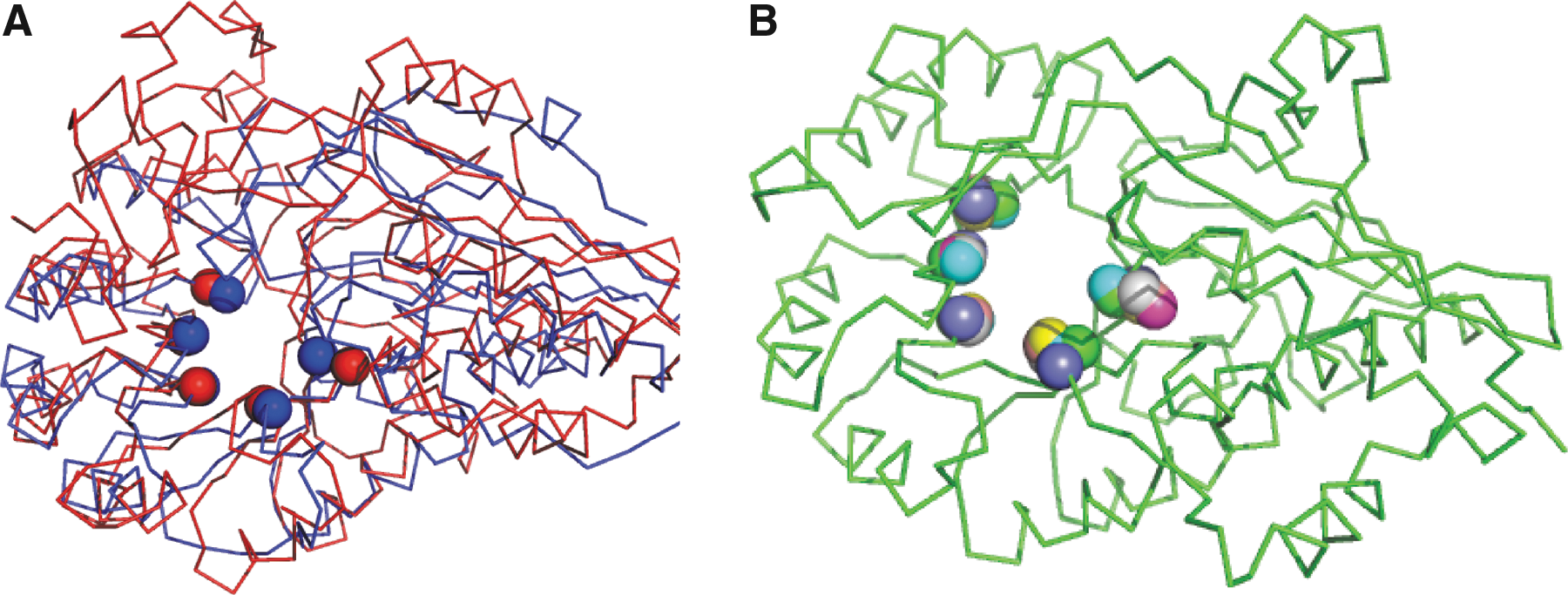
Enolase superfamily motif. (A) Two enolase superfamily structures (backbone trace) and their instances of a motif (C^α spheres) common to diverse members of this superfamily (Meng et al., 2004). Red: E. coli glucarate dehydratase (PDB ID 1ec7D); blue: E. coli O-succinylbenzoate synthase 2 (pdb id 1fhv). They have 19% sequence identity, and globally structurally align to ≈5 Å; the motif aligns to <1 Å. (B) Motif residues from seven templates superimposed on a mandelate racemase backbone (PDB ID 2mnrA). PDB, protein databank.

Structural motifs can better and more directly represent and utilize sequence-structure-function relationships than can alternative approaches such as sequence motifs and alignments and global structural alignments. Typical sequence motifs may not adequately capture a compact set of key functional residues, as such residues need not be nearby in the sequence. While sequence alignment methods can often be effectively used to identify evolutionarily related proteins, and phylogenetic analysis [e.g., orthology (Loewenstein et al., 2009)] can give further confidence in inferring related function, these techniques typically cannot help distinguish key functional residues from the overall background of evolutionarily related amino acids. They also have a hard time dealing with cases of limited sequence identity (as in the enolases in Fig. 1). Global structure alignment techniques can identify near and remote homologs and even unrelated proteins with similar overall three-dimensional structures, but do not directly separate key functional residues from the overall scaffold. These techniques can also have difficulties distinguishing functional subclasses within a superfamily (with the enolases once again providing an example).

Motif matching is (one name for) a core problem in structural motifs; the goal is to search for instances of a motif (query) in a set of protein structures (targets). Motif matching is a complex problem, with both a compositional and a geometric component. The compositional component requires residues in the motif to be matched with compatible residues (the same or similar amino acid types, in similar chemical environments, etc.). The geometric component requires the spatial distribution of motif residues to be similar to the spatial distribution of the matched residues. Often an additional statistical component, which is somewhat orthogonal to the actual matching problem itself, seeks to determine whether the match is likely to have occurred simply due to chance.

Numerous approaches for the motif-matching problem have been proposed (see Moll et al., 2010, for a good summary). Three approaches are fairly representative of the field and serve to establish the key contrasts in methodology.

Geometric hashing (Nussinov and Wolfson, 1991). This is one of the most-used methods for efficiently finding three-dimensional objects represented by discrete points that have undergone an affine transformation (Wolfson and Rigoutsos, 1997). The main idea is to preprocess the query and store its points (with labels for amino acid types, etc.) in a hash table, and to look up the targets against the hash table. The hashing and the look-up are performed by choosing sets of three points to define coordinate systems, and for each, transforming the remaining points accordingly, thereby defining rigid-body transformations that serve to align target points with query points. After its introduction in computer vision, this technique has been used in the development of many algorithms for structural biology, including motif analysis (Wallace et al., 1997; Barker and Thornton, 2003; Shulman-Peleg et al., 2004).

LabelHash (Moll et al., 2010). In contrast to geometric hashing, LabelHash hashes tuples of residues (typically three-tuples) from the target based on amino acid types rather than geometry, though each tuple does have to satisfy certain geometric constraints. Given a query, LabelHash looks up all matches to a submotif of the tuple size. It expands each partial match to a complete match using a depth-first search, a variant of the match augmentation algorithm (Chen et al., 2007). The residues added to a match during match augmentation are not subject to the geometric constraints of reference sets, and partial matches with root-mean-square deviation (RMSD) greater than a certain threshold are discarded.

Graph-based methods (Najmanovich et al., 2008; Bandyopadhyay et al., 2009). These and other graph-based approaches (e.g., Artymiuk et al., 1994; Gardiner et al., 1997; Milik et al., 2003; Wangikar et al., 2003) represent the query residues (or atoms) as vertices connected by edges for proximal pairs. In many cases, edges are defined by contact (e.g., based on a distance threshold), though Bandyopadhyay et al. (2009) derive the graphs from almost-Delaunay triangulations. In general, graph-based methods face the subgraph isomorphism problem, a well-known NP-complete problem (Ullmann, 1976). To tackle this, Bandyopadhyay et al. employ a heuristic that enables the search to be terminated when the local neighborhood of a subgraph is a witness to the impossibility of a match. Other graph-based methods formulate motif matching in terms of clique finding, though this is also NP-hard (Karp, 1972) and difficult to approximate (Feige et al., 1996). In IsoCleft (Najmanovich et al., 2008), cliques are found in a graph that has nodes for pairs of query and target residues with similar composition and edges for those pairs with similar geometry. A two-stage heuristic approach is then used to detect a match as the largest clique in this graph.

Despite the extensive amount of work on motif matching, it remains a challenge to efficiently identify all the instances of a structural motif in a database of protein structures (Moll et al., 2010). Since the protein databank (PDB) (Bernstein et al., 1977) has over 81,000 structures as of June 2012, efficiency is required.

Our contribution. We focus on the local geometric and compositional constraints defining a structural motif and derive a novel motif-matching approach called Ballast. Our approach combines the best properties of the previously proposed approaches: geometric hashing (geometric, but global), subgraph matching, and label hashing (local, but combinatorial). Ballast takes advantage of the locality of the residues in a structural motif and directly considers both geometry and composition (Fig. 2).

FIG. 2.

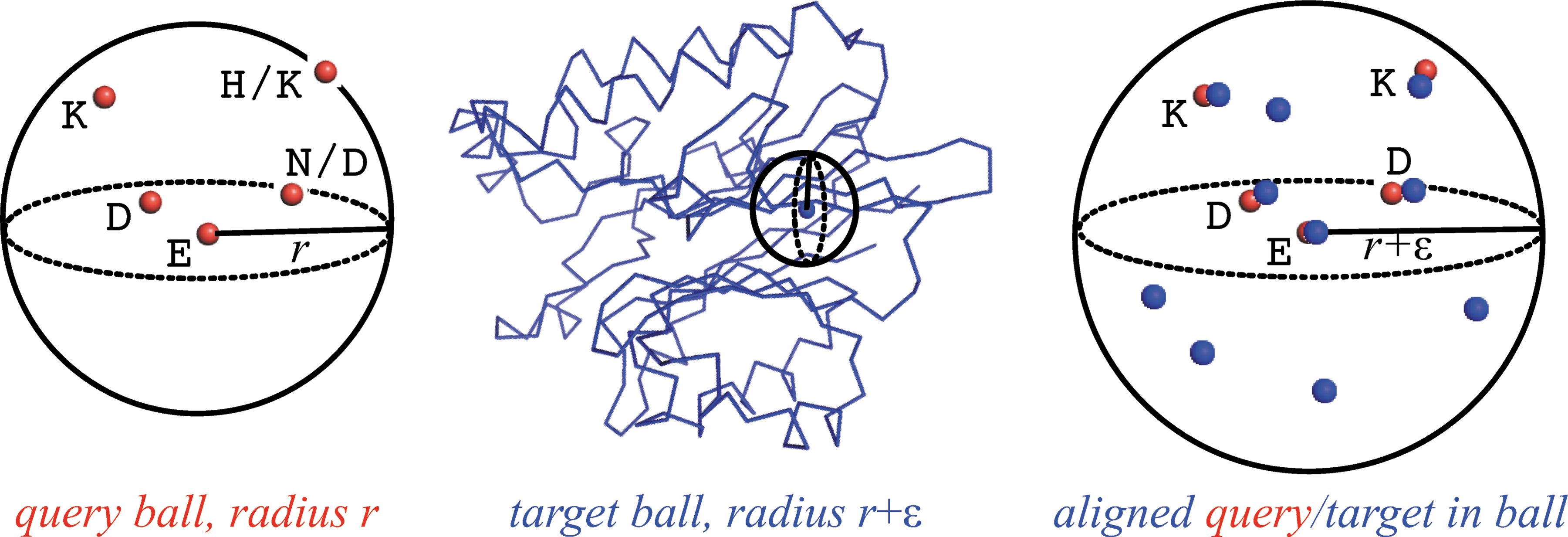
Ballast employs local (ball-based) matching to find in a target structure (blue) an instance of a query motif (red) defined in terms of a set of points (geometry, e.g., C^α coordinates) and labels (composition, e.g., allowed amino acids). A query ball is centered on one of the query points and contains the other points. An expanded target ball, with a larger radius to account for structural variation, is scanned through the target structure, centering it at each residue. If the target ball passes some filters (e.g., it contains a sufficient number of the query labels), then possible alignments between the query and target points are evaluated. The efficiency of Ballast stems from the fact that there are relatively few balls to consider, many of these are filtered, and the remaining ones have relatively few points to assess for matches.

We provide analytical evidence of the efficiency of Ballast, characterizing its performance under a suitable generative model for 3D structures. We derive an upper bound on the time complexity of our algorithm that holds with high probability and is substantially better than the complexity of other algorithms. We also provide empirical evidence of the efficiency and effectiveness of Ballast in practice. On a large and diverse set of previously studied motif-matching problems, it efficiently searches a large structural database. For those searches, the running time of Ballast is comparable to what was reported in Moll et al. (2010) for the state-of-the-art LabelHash code (though for different hardware), despite requiring no preprocessing or large index. Ballast is relatively unaffected by the number of motif points and scales well with the motif radius.

2. Problem Statement, Algorithm, and Analysis

We represent both motifs and target structures with labeled point sets. For the points, Ballast supports the commonly used representations of C^α, C^β, and side-chain centroid coordinates. For the labels on the points, Ballast currently supports amino acid types and is readily extensible to employ other (discrete) representations of composition (e.g., physicochemical classes). Sets of allowed labels may be provided for query points (i.e., possible amino acid types, allowing for substitution). More formally, we are given a query set \documentclass{aastex}\usepackage{amsbsy}\usepackage{amsfonts}\usepackage{amssymb}\usepackage{bm}\usepackage{mathrsfs}\usepackage{pifont}\usepackage{stmaryrd}\usepackage{textcomp}\usepackage{portland, xspace}\usepackage{amsmath, amsxtra}\pagestyle{empty}\DeclareMathSizes{10}{9}{7}{6}\begin{document} $$Q = \{ q_1 , q_2 , \ldots , q_k \} \subset {\mathbb R}^3$$ \end{document} of k points, and a target set \documentclass{aastex}\usepackage{amsbsy}\usepackage{amsfonts}\usepackage{amssymb}\usepackage{bm}\usepackage{mathrsfs}\usepackage{pifont}\usepackage{stmaryrd}\usepackage{textcomp}\usepackage{portland, xspace}\usepackage{amsmath, amsxtra}\pagestyle{empty}\DeclareMathSizes{10}{9}{7}{6}\begin{document} $$T \subset {\mathbb R}^3$$ \end{document} of n points (for a single structure at a time). We also have a function \documentclass{aastex}\usepackage{amsbsy}\usepackage{amsfonts}\usepackage{amssymb}\usepackage{bm}\usepackage{mathrsfs}\usepackage{pifont}\usepackage{stmaryrd}\usepackage{textcomp}\usepackage{portland, xspace}\usepackage{amsmath, amsxtra}\pagestyle{empty}\DeclareMathSizes{10}{9}{7}{6}\begin{document} $$A : Q \rightarrow 2^{ \cal A}$$ \end{document} mapping a query point to a set of allowed amino acids (from set \documentclass{aastex}\usepackage{amsbsy}\usepackage{amsfonts}\usepackage{amssymb}\usepackage{bm}\usepackage{mathrsfs}\usepackage{pifont}\usepackage{stmaryrd}\usepackage{textcomp}\usepackage{portland, xspace}\usepackage{amsmath, amsxtra}\pagestyle{empty}\DeclareMathSizes{10}{9}{7}{6}\begin{document} $${ \cal A} = \{ { \rm Ala} , { \rm Arg} , \ldots \} $$ \end{document} ), along with a function \documentclass{aastex}\usepackage{amsbsy}\usepackage{amsfonts}\usepackage{amssymb}\usepackage{bm}\usepackage{mathrsfs}\usepackage{pifont}\usepackage{stmaryrd}\usepackage{textcomp}\usepackage{portland, xspace}\usepackage{amsmath, amsxtra}\pagestyle{empty}\DeclareMathSizes{10}{9}{7}{6}\begin{document} $$a : T \rightarrow { \cal A}$$ \end{document} mapping a target point to its (single) amino acid in the structure.

Our goal is to find a subset M of T with ∣M∣=∣Q∣= k that matches Q. Many different geometric and compositional criteria have been considered in defining what constitutes a possible match and in evaluating these to select the best. For geometric evaluation, we focus here on the common RMSD criterion. Let v_M : Q → M be the bijection describing a possible match between Q and M. Then, \documentclass{aastex}\usepackage{amsbsy}\usepackage{amsfonts}\usepackage{amssymb}\usepackage{bm}\usepackage{mathrsfs}\usepackage{pifont}\usepackage{stmaryrd}\usepackage{textcomp}\usepackage{portland, xspace}\usepackage{amsmath, amsxtra}\pagestyle{empty}\DeclareMathSizes{10}{9}{7}{6}\begin{document} $$d_ { RMSD } ( M , Q ) = \sqrt { { \frac { 1 } { k } } \sum\nolimits_ { i = 1 } ^k \mid \mid q_i - v_M ( q_i ) \mid \mid ^2 } $$ \end{document} where ∥p − q∥ denotes the distance between points p and q. For compositional evaluation, we simply assess whether or not the target amino acids belong to the corresponding query sets. That is, \documentclass{aastex}\usepackage{amsbsy}\usepackage{amsfonts}\usepackage{amssymb}\usepackage{bm}\usepackage{mathrsfs}\usepackage{pifont}\usepackage{stmaryrd}\usepackage{textcomp}\usepackage{portland, xspace}\usepackage{amsmath, amsxtra}\pagestyle{empty}\DeclareMathSizes{10}{9}{7}{6}\begin{document} $$d_{AA} ( M , Q ) = \sum\nolimits_{i = 1}^k I \{ a ( v_M ( q_i ) ) \,\notin\, A ( q_i ) \} $$ \end{document} where I{·} is the indicator function. Ballast readily supports variations of these criteria (including distance differences and substitution scores), so we will continue to refer to geometric and compositional criteria generically. We consider a match to be a candidate if it satisfies constraints on the geometric and compositional criteria, namely that d_RMSD is at most a user-specified threshold θ and d_AA is zero (all amino acid types match).

Ballast assumes that a motif is both compact and relatively similar to the query. For compactness (see Fig. 2), we assume that there is a ball of radius r, centered on one of the points in Q and containing all of the points, such that r is “small” compared to the overall structure. For geometric similarity, we assume that for each pair of points in Q, the corresponding pair of points in T has about the same distance, within a user-specified parameter ɛ ≥ 0. Note that this is a local geometric constraint, somewhat complementary to the global RMSD constraint above; a candidate must satisfy both constraints. This further implies that the instance in the target fits within a ball of radius of at most r+ɛ when centered on one of the points in T. These assumptions, which also underlie graph-based methods, generally hold for structural motifs (particularly those defining catalytic sites), as we demonstrate in the results. We also show in the theoretical analysis below that they directly lead to the efficiency of Ballast. We note that r is part of the definition of a motif and follows from the given points, while ɛ is part of the definition of a match and is set by the user. In the results, we study the effects of ɛ on the output and efficiency.

The basic idea of our algorithm is straightforward (see Algorithm 1 and Fig. 2). We find the ball of minimum radius r, centered at some \documentclass{aastex}\usepackage{amsbsy}\usepackage{amsfonts}\usepackage{amssymb}\usepackage{bm}\usepackage{mathrsfs}\usepackage{pifont}\usepackage{stmaryrd}\usepackage{textcomp}\usepackage{portland, xspace}\usepackage{amsmath, amsxtra}\pagestyle{empty}\DeclareMathSizes{10}{9}{7}{6}\begin{document} $$\hat{q} \in Q$$ \end{document} , that contains all the points in query Q. Then we separately consider each point p in target T and examine the set of points B_p(r + ɛ) within the ball centered at p and of radius r+ɛ. We generate as candidate matches all the subsets of size k of B_p(r + ɛ) that contain p and satisfy the geometric and compositional constraints. While candidate generation could be done in a brute force fashion, we instead filter the possible matched target points for each query point to those correspondingly close to the center and of the corresponding amino acid type. We then take one point from each set, avoiding repetitions and ensuring satisfaction of the constraints. We show below that, while this generation step could be expensive, it is likely to be cheap due to the filtering, the locality, and compactness of the ball, and the physical nature of protein packing. Finally, we rank the candidates.

We now analyze the efficiency of Ballast. The ball of minimum radius r that contains all the points in Q (Lines 1, 2) can be found in time O (k²) by computing the O (k²) distances for all pairs of points in Q, and then finding for each point q in Q the maximum of the k − 1 distances between q and the other points in Q. The naive way to find all the points in B_p(r + ɛ) (Line 6) requires time O (n). This naive implementation is very efficient in practice and has been used in our experiments. However, we note that the complexity of this part can be improved employing a range tree (Lueker, 1978; Willard, 1978). A range tree is a data structure on n points (in 3D space) that can be built in time O (n log² n). It allows orthogonal range queries to be answered in time O (log²n + w), where w is the number of points reported. Since we want to find all the points in B_p(r + ɛ), we can first perform an orthogonal range query to retrieve all the points in the cube with edge length 2(r + ɛ) centered at p. Assuming there are w such points, then in time O (w) we can then find the ones in B_p(r + ɛ). For the generation of candidate matches (Lines 7–10), if we denote by m the number of points in B_p(r + ɛ), then in the worst case there are \documentclass{aastex}\usepackage{amsbsy}\usepackage{amsfonts}\usepackage{amssymb}\usepackage{bm}\usepackage{mathrsfs}\usepackage{pifont}\usepackage{stmaryrd}\usepackage{textcomp}\usepackage{portland, xspace}\usepackage{amsmath, amsxtra}\pagestyle{empty}\DeclareMathSizes{10}{9}{7}{6}\begin{document} $$m \choose k$$ \end{document} candidates; we tighten this in the corollary below, based on our geometric and compositional constraints. Thus the generation of candidate matches requires \documentclass{aastex}\usepackage{amsbsy}\usepackage{amsfonts}\usepackage{amssymb}\usepackage{bm}\usepackage{mathrsfs}\usepackage{pifont}\usepackage{stmaryrd}\usepackage{textcomp}\usepackage{portland, xspace}\usepackage{amsmath, amsxtra}\pagestyle{empty}\DeclareMathSizes{10}{9}{7}{6}\begin{document} $$O \; \left( {{m \choose k} \;f_c ( k ) } \right)$$ \end{document} time, where f_c(k) is the time required to evaluate a subset of k points for the constraints (instantiated for our constraints below). Therefore, the time complexity of our algorithm is \documentclass{aastex}\usepackage{amsbsy}\usepackage{amsfonts}\usepackage{amssymb}\usepackage{bm}\usepackage{mathrsfs}\usepackage{pifont}\usepackage{stmaryrd}\usepackage{textcomp}\usepackage{portland, xspace}\usepackage{amsmath, amsxtra}\pagestyle{empty}\DeclareMathSizes{10}{9}{7}{6}\begin{document} $$O \ \left( {k^2 + n \ \left( \log^2 n + w + {m \choose k} f_c ( k ) \right) } \right)$$ \end{document} .

Algorithm 1:

Pseudocode for algorithm Ballast.

	Input: Query set Q, target set T, radius expansion ɛ > 0, RMSD threshold θ
	Output: Candidate matches C ⊂ 2^T
1	\documentclass{aastex}\usepackage{amsbsy}\usepackage{amsfonts}\usepackage{amssymb}\usepackage{bm}\usepackage{mathrsfs}\usepackage{pifont}\usepackage{stmaryrd}\usepackage{textcomp}\usepackage{portland, xspace}\usepackage{amsmath, amsxtra}\pagestyle{empty}\DeclareMathSizes{10}{9}{7}{6}\begin{document} $$\hat {q} \leftarrow \arg \min \nolimits_{q \in Q} \max \{\mid \mid q - q_i \mid \mid : q_i \in Q \ \backslash \ \{ q \} \} $$ \end{document} ;
2	\documentclass{aastex}\usepackage{amsbsy}\usepackage{amsfonts}\usepackage{amssymb}\usepackage{bm}\usepackage{mathrsfs}\usepackage{pifont}\usepackage{stmaryrd}\usepackage{textcomp}\usepackage{portland, xspace}\usepackage{amsmath, amsxtra}\pagestyle{empty}\DeclareMathSizes{10}{9}{7}{6}\begin{document} $$r \leftarrow \max \{ \mid \mid \hat {q} - q_i \mid \mid : q_i \in Q \ \backslash \ \{ \hat {q} \} \} $$ \end{document} ;
3	C ← ∅;
4	for \documentclass{aastex}\usepackage{amsbsy}\usepackage{amsfonts}\usepackage{amssymb}\usepackage{bm}\usepackage{mathrsfs}\usepackage{pifont}\usepackage{stmaryrd}\usepackage{textcomp}\usepackage{portland, xspace}\usepackage{amsmath, amsxtra}\pagestyle{empty}\DeclareMathSizes{10}{9}{7}{6}\begin{document} $$p \in T$$ \end{document} do
5	if \documentclass{aastex}\usepackage{amsbsy}\usepackage{amsfonts}\usepackage{amssymb}\usepackage{bm}\usepackage{mathrsfs}\usepackage{pifont}\usepackage{stmaryrd}\usepackage{textcomp}\usepackage{portland, xspace}\usepackage{amsmath, amsxtra}\pagestyle{empty}\DeclareMathSizes{10}{9}{7}{6}\begin{document} $$a ( p ) \in A ( \hat {q} )$$ \end{document} then
6	\documentclass{aastex}\usepackage{amsbsy}\usepackage{amsfonts}\usepackage{amssymb}\usepackage{bm}\usepackage{mathrsfs}\usepackage{pifont}\usepackage{stmaryrd}\usepackage{textcomp}\usepackage{portland, xspace}\usepackage{amsmath, amsxtra}\pagestyle{empty}\DeclareMathSizes{10}{9}{7}{6}\begin{document} $$B_p ( r + \varepsilon ) \leftarrow \{ p^{ \prime} \in T \ \backslash \ \{ p \} : \mid \mid p - p^{ \prime} \mid \mid \leq r + \varepsilon \} $$ \end{document} ;
7	for \documentclass{aastex}\usepackage{amsbsy}\usepackage{amsfonts}\usepackage{amssymb}\usepackage{bm}\usepackage{mathrsfs}\usepackage{pifont}\usepackage{stmaryrd}\usepackage{textcomp}\usepackage{portland, xspace}\usepackage{amsmath, amsxtra}\pagestyle{empty}\DeclareMathSizes{10}{9}{7}{6}\begin{document} $$q_i \in Q \ \backslash \ \{ \hat {q} \} $$ \end{document} do
8	\documentclass{aastex}\usepackage{amsbsy}\usepackage{amsfonts}\usepackage{amssymb}\usepackage{bm}\usepackage{mathrsfs}\usepackage{pifont}\usepackage{stmaryrd}\usepackage{textcomp}\usepackage{portland, xspace}\usepackage{amsmath, amsxtra}\pagestyle{empty}\DeclareMathSizes{10}{9}{7}{6}\begin{document} $$d_i \leftarrow \mid \mid { \hat {q}} - q_i \mid \mid$$ \end{document} ;
9	\documentclass{aastex}\usepackage{amsbsy}\usepackage{amsfonts}\usepackage{amssymb}\usepackage{bm}\usepackage{mathrsfs}\usepackage{pifont}\usepackage{stmaryrd}\usepackage{textcomp}\usepackage{portland, xspace}\usepackage{amsmath, amsxtra}\pagestyle{empty}\DeclareMathSizes{10}{9}{7}{6}\begin{document} $$B_p^{ ( i ) } ( r + \varepsilon ) \leftarrow \{ p^{ \prime} \in B_p ( r + \varepsilon ) : a ( p^{ \prime} ) \in A ( q_i ) , \mid \mid p - p^{ \prime} \mid \mid \in [ d_i - \varepsilon , d_i + \varepsilon ] \} $$ \end{document} ;
10	\documentclass{aastex}\usepackage{amsbsy}\usepackage{amsfonts}\usepackage{amssymb}\usepackage{bm}\usepackage{mathrsfs}\usepackage{pifont}\usepackage{stmaryrd}\usepackage{textcomp}\usepackage{portland, xspace}\usepackage{amsmath, amsxtra}\pagestyle{empty}\DeclareMathSizes{10}{9}{7}{6}\begin{document} $$C \leftarrow C \cup \{ M \in \prod \nolimits_i B_p^{ ( i ) } ( r + \varepsilon )$$ \end{document} : M has no repeats, d_RMSD (M, Q) < θ, \documentclass{aastex}\usepackage{amsbsy}\usepackage{amsfonts}\usepackage{amssymb}\usepackage{bm}\usepackage{mathrsfs}\usepackage{pifont}\usepackage{stmaryrd}\usepackage{textcomp}\usepackage{portland, xspace}\usepackage{amsmath, amsxtra}\pagestyle{empty}\DeclareMathSizes{10}{9}{7}{6}\begin{document} $$\qquad\ \ \ \qquad\forall q \neq q^{ \prime} \in Q : \mid \mid \mid q - q^{ \prime} \mid \mid - \mid \mid v_M ( q ) - v_M ( q^{ \prime} ) \mid \mid \mid \leq \varepsilon \} $$ \end{document} ;
11	Sort C by geometric and compositional criteria;
12	return C;

The efficiency of our algorithm strongly depends on the number m of points that are found in B_p(r + ɛ). In the worst case, m could be as large as n, and thus our algorithm could require Ω (n^k) time, but in practice our method is extremely efficient. To understand why, we analyze the performance of our algorithm when the input is not adversarially chosen, but when the points in T are drawn from a probability distribution. This distribution is the same considered for the G(n, r, ℓ) random geometric graph model (Muthukrishnan and Pandurangan, 2005), a generalization of the G(n, r) random geometric graph model (Penrose, 2003) that scales to arbitrary sizes. In the G(n, r, ℓ) model, the vertices are points placed uniformly at random in [0, ℓ]³. We present a probabilistic analysis to show that the average case performance of the algorithm is good; this provides a theoretical insight as to why the algorithm works efficiently in practice.

We now prove that if the points in T are drawn uniformly at random in [0, ℓ]³, and for reasonable values of the parameters r and ɛ, the number of points inside B_p(r + ɛ) is small whp.¹

Lemma 2.1

Let T be a set of n points drawn uniformly at random from [0, ℓ]³ and r, ɛ ≥ 0 such that \documentclass{aastex}\usepackage{amsbsy}\usepackage{amsfonts}\usepackage{amssymb}\usepackage{bm}\usepackage{mathrsfs}\usepackage{pifont}\usepackage{stmaryrd}\usepackage{textcomp}\usepackage{portland, xspace}\usepackage{amsmath, amsxtra}\pagestyle{empty}\DeclareMathSizes{10}{9}{7}{6}\begin{document} $$r + \varepsilon \in O \ \left( \ell ( \frac { { \log n } } { n } ) ^ { 1 / 3 } \right)$$ \end{document} . Then \documentclass{aastex}\usepackage{amsbsy}\usepackage{amsfonts}\usepackage{amssymb}\usepackage{bm}\usepackage{mathrsfs}\usepackage{pifont}\usepackage{stmaryrd}\usepackage{textcomp}\usepackage{portland, xspace}\usepackage{amsmath, amsxtra}\pagestyle{empty}\DeclareMathSizes{10}{9}{7}{6}\begin{document} $$m = \max \nolimits_{p \in T} \{ \mid B_p ( r + \varepsilon ) \mid \} \in O \ ( \log n )$$ \end{document} whp.

Proof

Consider a point \documentclass{aastex}\usepackage{amsbsy}\usepackage{amsfonts}\usepackage{amssymb}\usepackage{bm}\usepackage{mathrsfs}\usepackage{pifont}\usepackage{stmaryrd}\usepackage{textcomp}\usepackage{portland, xspace}\usepackage{amsmath, amsxtra}\pagestyle{empty}\DeclareMathSizes{10}{9}{7}{6}\begin{document} $$p \in T$$ \end{document} . Let E be the event “a point drawn uniformly at random from [0, ℓ]³ is at distance at most r + ɛ from p.” Since \documentclass{aastex}\usepackage{amsbsy}\usepackage{amsfonts}\usepackage{amssymb}\usepackage{bm}\usepackage{mathrsfs}\usepackage{pifont}\usepackage{stmaryrd}\usepackage{textcomp}\usepackage{portland, xspace}\usepackage{amsmath, amsxtra}\pagestyle{empty}\DeclareMathSizes{10}{9}{7}{6}\begin{document} $$r + \varepsilon \in O \ \left( { \ell ( \frac { { \log n } } { n } ) ^ { 1 / 3 } } \right)$$ \end{document} , we have \documentclass{aastex}\usepackage{amsbsy}\usepackage{amsfonts}\usepackage{amssymb}\usepackage{bm}\usepackage{mathrsfs}\usepackage{pifont}\usepackage{stmaryrd}\usepackage{textcomp}\usepackage{portland, xspace}\usepackage{amsmath, amsxtra}\pagestyle{empty}\DeclareMathSizes{10}{9}{7}{6}\begin{document} $$ { \bf Pr } [ { E } ] \le c_1 \frac { { \log n } } { n } $$ \end{document} , for a suitable constant c₁.

Thus we can bound the expected number of points in B_p(r + ɛ): \documentclass{aastex}\usepackage{amsbsy}\usepackage{amsfonts}\usepackage{amssymb}\usepackage{bm}\usepackage{mathrsfs}\usepackage{pifont}\usepackage{stmaryrd}\usepackage{textcomp}\usepackage{portland, xspace}\usepackage{amsmath, amsxtra}\pagestyle{empty}\DeclareMathSizes{10}{9}{7}{6}\begin{document} \begin{align}\mu = { \bf E } [ \mid B_p ( r + \varepsilon ) \mid \le n c_1 \frac { { \log n } \ } { n } = c_1 \log n.\end{align} \end{document}

Now fix a constant c₂ > 3c₁. By Chernoff bound (Mitzenmacher and Upfal, 2005) with δ = c₂/c₁ − 1 we have: \documentclass{aastex}\usepackage{amsbsy}\usepackage{amsfonts}\usepackage{amssymb}\usepackage{bm}\usepackage{mathrsfs}\usepackage{pifont}\usepackage{stmaryrd}\usepackage{textcomp}\usepackage{portland, xspace}\usepackage{amsmath, amsxtra}\pagestyle{empty}\DeclareMathSizes{10}{9}{7}{6}\begin{document} \begin{align} { \bf Pr } [ \mid B_p ( r + \varepsilon ) \mid \ge c_2 \log n ] & \,= \, { \bf Pr } [ \mid B_p ( r + \varepsilon ) \mid \ge ( 1 + \delta ) \mu ] \\ & \le e^ { - \frac { \delta^2 \mu } { 3 } } \\ & \le e^ { - d \log n } \\ & \le \frac { 1 } { n^ { d } } \end{align} \end{document}

for a constant d > 1. Then, applying the union bound on all points \documentclass{aastex}\usepackage{amsbsy}\usepackage{amsfonts}\usepackage{amssymb}\usepackage{bm}\usepackage{mathrsfs}\usepackage{pifont}\usepackage{stmaryrd}\usepackage{textcomp}\usepackage{portland, xspace}\usepackage{amsmath, amsxtra}\pagestyle{empty}\DeclareMathSizes{10}{9}{7}{6}\begin{document} $$p \in T$$ \end{document} , we have that: \documentclass{aastex}\usepackage{amsbsy}\usepackage{amsfonts}\usepackage{amssymb}\usepackage{bm}\usepackage{mathrsfs}\usepackage{pifont}\usepackage{stmaryrd}\usepackage{textcomp}\usepackage{portland, xspace}\usepackage{amsmath, amsxtra}\pagestyle{empty}\DeclareMathSizes{10}{9}{7}{6}\begin{document} \begin{align} { \bf Pr } [ \exists p: \mid B_p ( r + \varepsilon ) \mid \ge c_2 \log n ] \le n \frac { 1 } { n^ { d } } \le \frac { 1 } { n^ { d - 1 } } \end{align} \end{document}

for n sufficiently large, that is \documentclass{aastex}\usepackage{amsbsy}\usepackage{amsfonts}\usepackage{amssymb}\usepackage{bm}\usepackage{mathrsfs}\usepackage{pifont}\usepackage{stmaryrd}\usepackage{textcomp}\usepackage{portland, xspace}\usepackage{amsmath, amsxtra}\pagestyle{empty}\DeclareMathSizes{10}{9}{7}{6}\begin{document} $$m \in O \ ( \log \, n )$$ \end{document} whp. ■

Lemma 2.1 gives theoretical evidence of why the use of a ball results in an efficient approach: Since “few” residues are found in a ball whp. when the residues are placed randomly, few subsets are considered for candidate generation and hence few candidates are explicitly examined. We can use this to bound the overall time complexity.

Theorem 2.2

Let T be a set of n points drawn uniformly at random from [0, ℓ]³, Q a set of \documentclass{aastex}\usepackage{amsbsy}\usepackage{amsfonts}\usepackage{amssymb}\usepackage{bm}\usepackage{mathrsfs}\usepackage{pifont}\usepackage{stmaryrd}\usepackage{textcomp}\usepackage{portland, xspace}\usepackage{amsmath, amsxtra}\pagestyle{empty}\DeclareMathSizes{10}{9}{7}{6}\begin{document} $$k \in o ( \log \, n )$$ \end{document} points and r, ɛ ≥ 0 such that \documentclass{aastex}\usepackage{amsbsy}\usepackage{amsfonts}\usepackage{amssymb}\usepackage{bm}\usepackage{mathrsfs}\usepackage{pifont}\usepackage{stmaryrd}\usepackage{textcomp}\usepackage{portland, xspace}\usepackage{amsmath, amsxtra}\pagestyle{empty}\DeclareMathSizes{10}{9}{7}{6}\begin{document} $$r + \varepsilon \in O \ \left( { \ell ( \frac { { \log n } } { n } ) ^ { 1 / 3 } } \right)$$ \end{document} . Then for any (small) constant d > 0 the time complexity of our algorithm is bounded by O (n^1+d f_c(k)) whp.

Proof

From Lemma 2.1 \documentclass{aastex}\usepackage{amsbsy}\usepackage{amsfonts}\usepackage{amssymb}\usepackage{bm}\usepackage{mathrsfs}\usepackage{pifont}\usepackage{stmaryrd}\usepackage{textcomp}\usepackage{portland, xspace}\usepackage{amsmath, amsxtra}\pagestyle{empty}\DeclareMathSizes{10}{9}{7}{6}\begin{document} $$m \in O \ ( \log \, n )$$ \end{document} whp, that is m ≤ c log n for a certain constant c > 0. Since k = o (log n), there exists a function g(n) such that \documentclass{aastex}\usepackage{amsbsy}\usepackage{amsfonts}\usepackage{amssymb}\usepackage{bm}\usepackage{mathrsfs}\usepackage{pifont}\usepackage{stmaryrd}\usepackage{textcomp}\usepackage{portland, xspace}\usepackage{amsmath, amsxtra}\pagestyle{empty}\DeclareMathSizes{10}{9}{7}{6}\begin{document} $$\displaystyle \lim_ { n \rightarrow \infty } \frac { k } { \log n } = \frac { 1 } { g ( n ) } \rightarrow 0$$ \end{document} , that is g(n) → ∞ for n → ∞ and \documentclass{aastex}\usepackage{amsbsy}\usepackage{amsfonts}\usepackage{amssymb}\usepackage{bm}\usepackage{mathrsfs}\usepackage{pifont}\usepackage{stmaryrd}\usepackage{textcomp}\usepackage{portland, xspace}\usepackage{amsmath, amsxtra}\pagestyle{empty}\DeclareMathSizes{10}{9}{7}{6}\begin{document} $$k \le \frac { \log n } { g ( n ) } $$ \end{document} for n sufficiently large. Thus, for n sufficiently large we have \documentclass{aastex}\usepackage{amsbsy}\usepackage{amsfonts}\usepackage{amssymb}\usepackage{bm}\usepackage{mathrsfs}\usepackage{pifont}\usepackage{stmaryrd}\usepackage{textcomp}\usepackage{portland, xspace}\usepackage{amsmath, amsxtra}\pagestyle{empty}\DeclareMathSizes{10}{9}{7}{6}\begin{document} \begin{align} { m \choose k } & \le \left( \frac { { c e \log n } } { k } \right) ^k \\ & \le \left( { \frac { c e \log n } { \log n / g ( n ) } } \right) ^ { \log n / g ( n ) } \\ & \le \left( c e \right) ^ { \log n / g ( n ) } \left( g ( n ) \right) ^ { \log n / g ( n ) } . \end{align} \end{document}

Note that for any (small) constant d > 0, we have \documentclass{aastex}\usepackage{amsbsy}\usepackage{amsfonts}\usepackage{amssymb}\usepackage{bm}\usepackage{mathrsfs}\usepackage{pifont}\usepackage{stmaryrd}\usepackage{textcomp}\usepackage{portland, xspace}\usepackage{amsmath, amsxtra}\pagestyle{empty}\DeclareMathSizes{10}{9}{7}{6}\begin{document} $$\left( c e \right) ^{ \log n / g ( n ) } \in O \ { ( n^{d / 2} ) }$$ \end{document} and \documentclass{aastex}\usepackage{amsbsy}\usepackage{amsfonts}\usepackage{amssymb}\usepackage{bm}\usepackage{mathrsfs}\usepackage{pifont}\usepackage{stmaryrd}\usepackage{textcomp}\usepackage{portland, xspace}\usepackage{amsmath, amsxtra}\pagestyle{empty}\DeclareMathSizes{10}{9}{7}{6}\begin{document} $$\left( g ( n ) \right) ^{ \log n / g ( n ) } \in O \ { ( n^{d / 2} ) }$$ \end{document} . Thus we have \documentclass{aastex}\usepackage{amsbsy}\usepackage{amsfonts}\usepackage{amssymb}\usepackage{bm}\usepackage{mathrsfs}\usepackage{pifont}\usepackage{stmaryrd}\usepackage{textcomp}\usepackage{portland, xspace}\usepackage{amsmath, amsxtra}\pagestyle{empty}\DeclareMathSizes{10}{9}{7}{6}\begin{document} \begin{align}{m \choose k} \le \left( c e \right) ^{ \log n / g ( n ) } \left( g ( n ) \right) ^{ \log n / g ( n ) } \in O \ { ( n^d ) }\end{align} \end{document}

for any (small) constant d > 0. Note that the analysis of Lemma 2.1 holds if we consider the event E as “a point drawn uniformly at random from [0, ℓ]³ is in the cube of edge 2(r + ɛ) centered in p.” Thus, w is O (log n), and the theorem follows. ■

The complexity of our approach depends on the effectiveness in the constraints used to filter candidates (through f_c(k)). We now obtain a more precise analysis by incorporating the constraints in our current implementation. Note that the rigid superposition to evaluate d_RMSD(M, Q) can be computed in time O (k) (Arun et al., 1987), and that the time complexity to check if M satisfies pairwise distances and allows amino acids substitutions constraints is O (k²). Thus, in this case we have \documentclass{aastex}\usepackage{amsbsy}\usepackage{amsfonts}\usepackage{amssymb}\usepackage{bm}\usepackage{mathrsfs}\usepackage{pifont}\usepackage{stmaryrd}\usepackage{textcomp}\usepackage{portland, xspace}\usepackage{amsmath, amsxtra}\pagestyle{empty}\DeclareMathSizes{10}{9}{7}{6}\begin{document} $$f_c ( k ) \in O \ { ( k^2 ) }$$ \end{document} .

Corollary 2.3

Let T be a set of n points drawn uniformly at random from [0, 1]³, Q a set of \documentclass{aastex}\usepackage{amsbsy}\usepackage{amsfonts}\usepackage{amssymb}\usepackage{bm}\usepackage{mathrsfs}\usepackage{pifont}\usepackage{stmaryrd}\usepackage{textcomp}\usepackage{portland, xspace}\usepackage{amsmath, amsxtra}\pagestyle{empty}\DeclareMathSizes{10}{9}{7}{6}\begin{document} $$k \in o \ ( \log n )$$ \end{document} points, and ɛ ≥ 0 such that \documentclass{aastex}\usepackage{amsbsy}\usepackage{amsfonts}\usepackage{amssymb}\usepackage{bm}\usepackage{mathrsfs}\usepackage{pifont}\usepackage{stmaryrd}\usepackage{textcomp}\usepackage{portland, xspace}\usepackage{amsmath, amsxtra}\pagestyle{empty}\DeclareMathSizes{10}{9}{7}{6}\begin{document} $$r + \varepsilon \in O \ ( { n^{ - 1 / 3}} )$$ \end{document} . If we look for matches satisfying our constraints (maximum RMSD of θ, matching amino acid types, and maximum pairwise distance expansion of ε), the time complexity of algorithm is bounded by o (n^1+d log²n) whp. for any (small) constant d > 0.

It follows that Ballast is more efficient than previous motif-matching approaches. Geometric hashing. All possible bases of 3 points in T are considered, and the points in T are transformed to each such basis. Since there are Θ (n³) such bases and each transformation requires time Θ (n), the total complexity is Θ (n⁴). LabelHash. For a new protein target T, LabelHash starts with “reference sets,” all 3-tuples from T, as possible seeds for matching, and then augments them to full-size matches. Thus, the time complexity is at least Θ (n³). This is of course a loose characterization, since it does not take into account the augmentation phase. (For a fixed target, the LabelHash index avoids the recomputation of the reference sets of the target. A similar strategy could be used with our approach, e.g., precomputing the points inside B_p(r + ɛ) for each point p in each target structure, for different values of r and ɛ.) Graph-based methods. Even before tackling the NP-hard subgraph isomorphism, Bandyopadhyay et al. (2009) compute an almost-Delaunay triangulation. The proposed algorithm (Bandyopadhyay and Snoeyink, 2004) requires time O (n⁵ log n) in the worst case, but runs in O (n² log n) expected time (no result whp. is proved). IsoCleft (Najmanovich et al., 2008) uses the Bron and Kerbosch algorithm (Bron and Kerbosch, 1973) to detect the largest clique, which can take up to O (3^n/3) time.

3. Results

In order to assess the practical utility of Ballast, we applied it to a wide range of matching problems previously studied by LabelHash (Moll et al., 2010). Two case studies enable us to explore the matching of structural motifs initially defined from structural analysis (enolases; Meng et al., 2004) and sequence analysis (SOIPPA; Xie and Bourne, 2008). A set of 147 motifs derived from the Catalytic Site Atlas (CSA; Porter et al., 2004) are not so rigorously characterized but serve as a large-scale benchmark.

Since Ballast addresses the motif-matching problem rather than the motif-discovery problem, we focus on its performance in finding motifs, not on the significance of the motifs themselves (e.g., by assessing the p-values under some null model). Ballast is guaranteed to find all instances satisfying the definition of a motif and the settings of the ɛ (local distance expansion) and θ (global RMSD) parameters. In order to analyze the structural variability underlying the motif, and the effects of the geometric constraints, we vary these parameters and characterize the numbers of matches in the “foreground” dataset used to develop the motif (essentially a sensitivity measure) as well as in a large “background” dataset of structures (specificity). The case study-specific foregrounds are introduced below. For the background, we used 30111 non redundant protein structures from the PDB, clustered by BLASTClust at 95% sequence identity.

Moll et al. (2010) performed an extensive evaluation of the performance of LabelHash, including its scalability with multiple cores. Our current implementation of Ballast is in single-threaded Java code, but is embarrassingly parallel and could easily be extended to distribute different subsets of the target database to different cores. For now, we simply study the single-core performance of Ballast in searching our 30111-member background database, analyzing the dependence on ɛ. There is no need to study the effects of θ on the time required by Ballast, as θ is an RMSD threshold only applied in a post-processing step to filter the candidate matches; the choice of threshold value does not impact the running time.

Results are provided in terms of wall-clock time on a Linux machine with an AMD Opteron 2435 processor and 32 GB memory (though we do not require or utilize large memory).

We do not present a direct performance comparison against LabelHash since we run Ballast on different hardware and a different background dataset from that reported for LabelHash (Moll et al., 2010; 21745 structures, roughly 2/3 our background). Indeed, our purpose is only to show that the current straightforward implementation of Ballast has reasonable performance, comparable to other, highly optimized tools. We do see in all our test cases that the wall-clock times are fairly comparable, on the same order of magnitude (though again with different hardware). We have an advantage when motifs have more points; they have an advantage when the amino acid labels are unambiguous. As we have emphasized throughout, our key contribution is a new algorithmic framework that combines locality and geometry, and provides a strong theoretical rationale for efficient performance. We also note that, as part of its simplicity, Ballast requires no extra data structures and only preprocesses the PDB files into binary files in order to speed the loading time (a few MB extra). In contrast, LabelHash employs a preprocessed 9.5 GB hash table for a 21745-structure background, which increases to 65 GB when considering the entire PDB; as reported (Moll et al., 2010), this number would grow to approximately 5 TB with reference sets of size 4.

3.1. Enolase superfamily

The enolase superfamily (ES) includes seven major subgroups that share core catalytic sites supporting the abstraction of a proton from a carbon adjacent to a carboxylic acid, in order to form an enolate anion intermediate (Babbitt et al., 1996). Enzymes in the superfamily have in common two domains, an N-terminal capping domain for substrate specificity and a C-terminal TIM beta/alpha-barrel domain containing key catalytic residues at the ends of the beta strands. A five-residue structural motif common to the superfamily was developed by Meng et al. (2004) based on seven representative structure templates (Fig. 1). Using residue numbering based on mandelate racemase (PDB id 2MNR) and listing multiple allowed amino acid types where appropriate, the ES motif includes KH164, D195, E221, EDN247, and HK297; we note that according to the structure-function linkage database (Pegg et al., 2006), there is some ambiguity in the first position. As the superfamily is known to have particularly diverse structures in terms of C^α RMSDs, side-chain centroids were instead used to define the motif geometry. While Meng et al. originally used SPASM (Kleywegt, 1999) for motif matching, Moll et al. (2010) demonstrated that LabelHash could also successfully match it against the superfamily members.

We used Ballast to search for instances of the ES motif in a foreground ES family benchmark of 77 chains provided by Meng et al. (excluding the one with no PDB code). The top part of Figure 3 illustrates the number of matches found in both the superfamily and background under different settings of the parameters. We reemphasize that Ballast is complete with respect to the parameter values, so this analysis is a characterization of the quality of the motif rather than the quality of the algorithm. That is, the efficiency of Ballast enables us to characterize the structural variability over the instances of a motif and the effects on sensitivity and specificity in trying to account for that variability by allowing some local and global geometric “slop.” We find that the enolase motif is rather robust. The foreground requires an RMSD of 1 Å or more to allow for variation among instances of the motif. The pairwise distances can vary by around 2 Å but are relatively stable with any ɛ at least that large. Looser settings also lead to the identification of multiple instances in some of the foreground structures, though we only report one match per structure in the figure. With RMSD at 1 Å and ɛ at 2 Å, we find 66 of the 77 foreground matches. Six of the missing ones require an RMSD of 1.1 Å, and one also requires ɛ of 3 Å. The remaining four all belong to the subfamily of methylaspartate ammonialyase, which is apparently more structurally variable, requiring RMSD of 1.5 Å and ɛ of 4 Å.

FIG. 3.
Matches found by Ballast in the foreground and background for enolases and SOIPPA-derived motifs (identified by PDB ID), under different values for ɛ (x-axis) and RMSD threshold (different lines, red: 0.5; blue: 1.0; magenta: 1.5; green: 2.0). The foreground sizes are indicated by black dashed horizontal lines; the background size, not shown, is roughly 30111, though we excluded foreground structures. SOIPPA, sequence Order-Independent Profile-Profile Alignment (SOIPPA) method; RMSD, root-mean-square deviation.

There are relatively few instances of the ES motif in the background. With the basic settings (RMSD: 1 Å, ɛ: 2 Å) required to achieve reasonable foreground coverage (66/77, 86%), there are only 68 nonforeground matches among the 30100 background structures (0.23%), excluding 11 structures in the foreground. Of those, 22 were not in the original foreground dataset but actually do belong to the enolase superfamily according to the structure–function linkage database (Pegg et al., 2006). The remaining 46 are not known to be ES members although many have very good instances of the motif (19 with RMSDs ≤ 0.5 Å). Bumping the RMSD up to 1.5 Å while holding ɛ at 2 Å yields better sensitivity (72/77, 93.5%) at the price of some additional background hits (total of 82, 0.27%, with 23 not in the foreground but in the superfamily). Increasing ɛ at the higher RMSD threshold has detrimental effects on specificity. Thus, Ballast enables us to conclude that the ES motif provides a fairly “tight” specification of the structural pattern common to the superfamily and distinct from other structures.

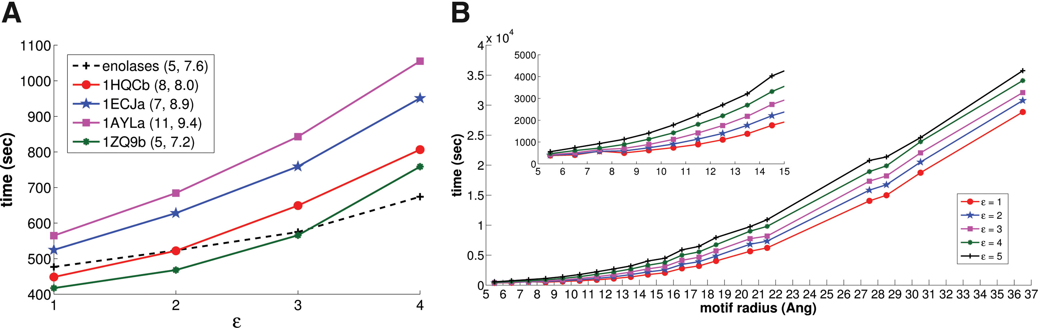
The dashed line in Figure 4 (left) characterizes the running time of Ballast for the background search at different ɛ values. While increasing the distance expansion parameter results in a larger ball size and more potential matches to assess, even the 4 Å setting only requires an additional 197 seconds beyond that for the baseline 1 Å. In terms of a rough comparison of wall-clock times (on different hardware; see the start of the Results for a discussion), we note that LabelHash (Moll et al., 2010) reported roughly 1000 seconds for a background search, about twice as long as Ballast.

FIG. 4.
Wall-clock timing results for Ballast background searches. (A) ES motif (dashed lines) and SOIPPA-derived motifs (solid), with varying ɛ (x-axis). In the legend, each motif is characterized by (# points, radius). (B) Averages over motifs in the Catalytic Site Atlas (CSA) database, grouped by radius (within ±0.5 Å, at different ɛ values [lines].

3.2. SOIPPA-derived motifs

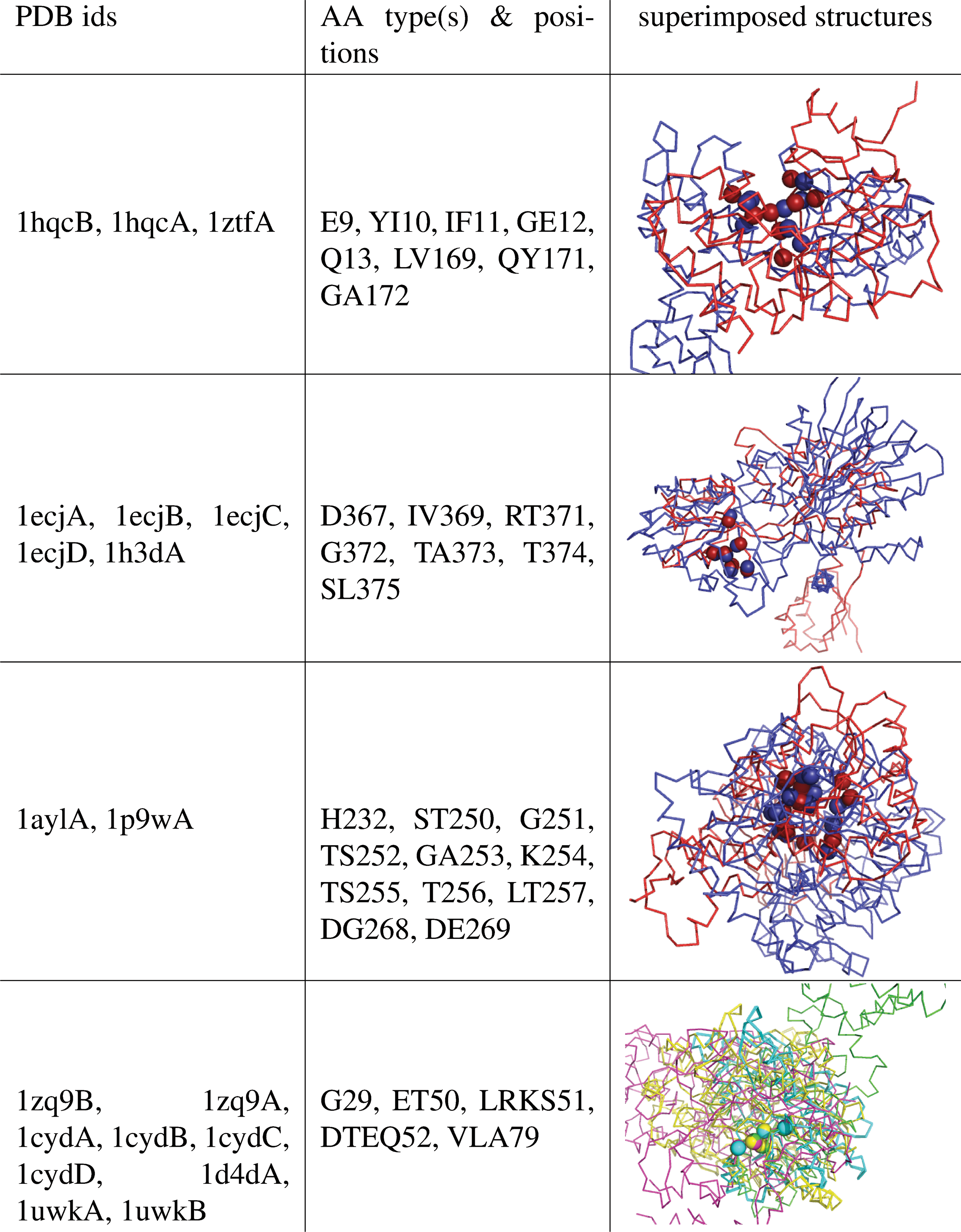
Xie and Bourne (2008) developed the Sequence Order–Independent Profile–Profile Alignment (SOIPPA) method to align protein structures independent of the sequential order of the residues, and identify motifs with similar local structures but distinct sequences. Moll et al. (2010) derived structural motifs from SOIPPA motifs by, for each SOIPPA motif, using the C^α coordinates from one template structure, along with all SOIPPA-identified alternative amino acid types. Motif details are provided in Figure 5; note that some motifs show up in multiple chains.

FIG. 5.
SOIPPA-derived motifs.

As discussed, Ballast enables us to evaluate the robustness of a motif by performing searches at different threshold values and thereby assessing structural variability in terms of these local (ɛ) and global (RMSD) parameters. We matched each motif against a foreground dataset consisting of the original SOIPPA-aligned structures, as well the entire background database; the bottom part of Figure 3 summarizes the numbers of matches. Note that the motifs show up multiple times in some of the foreground structures; each is counted separately in these figures. The different foreground datasets clearly have different levels of structural diversity, as might be expected from motifs initially derived from sequence profiles. For example, 1zq9B is very “tight,” with the entire foreground covered at any setting of the parameters and hitting only 19 background structures with, e.g., ɛ of 1 Å and RMSD of 0.5 Å. 1ecjA is also quite tight, with ɛ of 2 Å and RMSD of 1 Å covering the entire foreground and only three members of the background. It also remains quite stable to background hits with increasing ɛ under the smaller RMSD thresholds. On the other hand, we need ɛ of 4 Å and RMSD of 2 Å to cover the foregrounds for 1hqcB and 1aylA, hitting respectively 16 matches in 13 unique chains (1hqcB) and 36 in 15 (1aylA). In the case of 1hqcB, the two chains of 1hqc are covered before the other foreground chain. Again we see the power of Ballast in performing a range of motif searches and helping characterize the trade-offs required to account for structural variability.

Efficiency wise, our implementation took less than 1100 seconds of wall-clock time to match each motif against the background database even with ɛ set to 4 Å (Fig. 4, left). The motifs range from 5 residues up to 11 residues and about 7.2 Å to 9.4 Å in ball radius, with the larger ones taking a bit longer. We see good scalability over the ɛ range. 1zq9b suffers the largest loss due to the extra time for outputting the large number of matches. These numbers again compare very favorably to those reported by LabelHash (though again on different hardware with a different background), which exceed 5000 seconds. This is because the LabelHash hash keys are typically for only three residues, and the extension from the quick identification of those “core” sets to an entire motif (of up to 11 points) is relatively expensive. In contrast, Ballast simultaneously filters on both geometry and amino acid content. This same contrast holds for graph-based approaches, as subgraph isomorphism scales poorly with subgraph size.

3.3. Catalytic Site Atlas

The Catalytic Site Atlas (CSA) (Porter et al., 2004) defines residues implicated as comprising catalytic sites for a range of families. Moll et al. (2010) constructed 147 motifs from 147 CSA sites within 118 unique EC classes spanning 6 top-level EC classifications (oxidoreductases, transferases, hydrolases, lyases, isomerases, and ligases). Each motif was defined using the C^α geometry and amino acid types for a single representative structure, due to the lack of characterized substitutions and alignments. We followed the same procedure to generate an analogous dataset, though note that the actual members may be different from those used by Moll et al. (2010) (and we do have different sizes of the foreground sets), due to changing databases and so forth. The task is then to search each motif against a foreground comprising the members of the corresponding EC family, as well as the background.

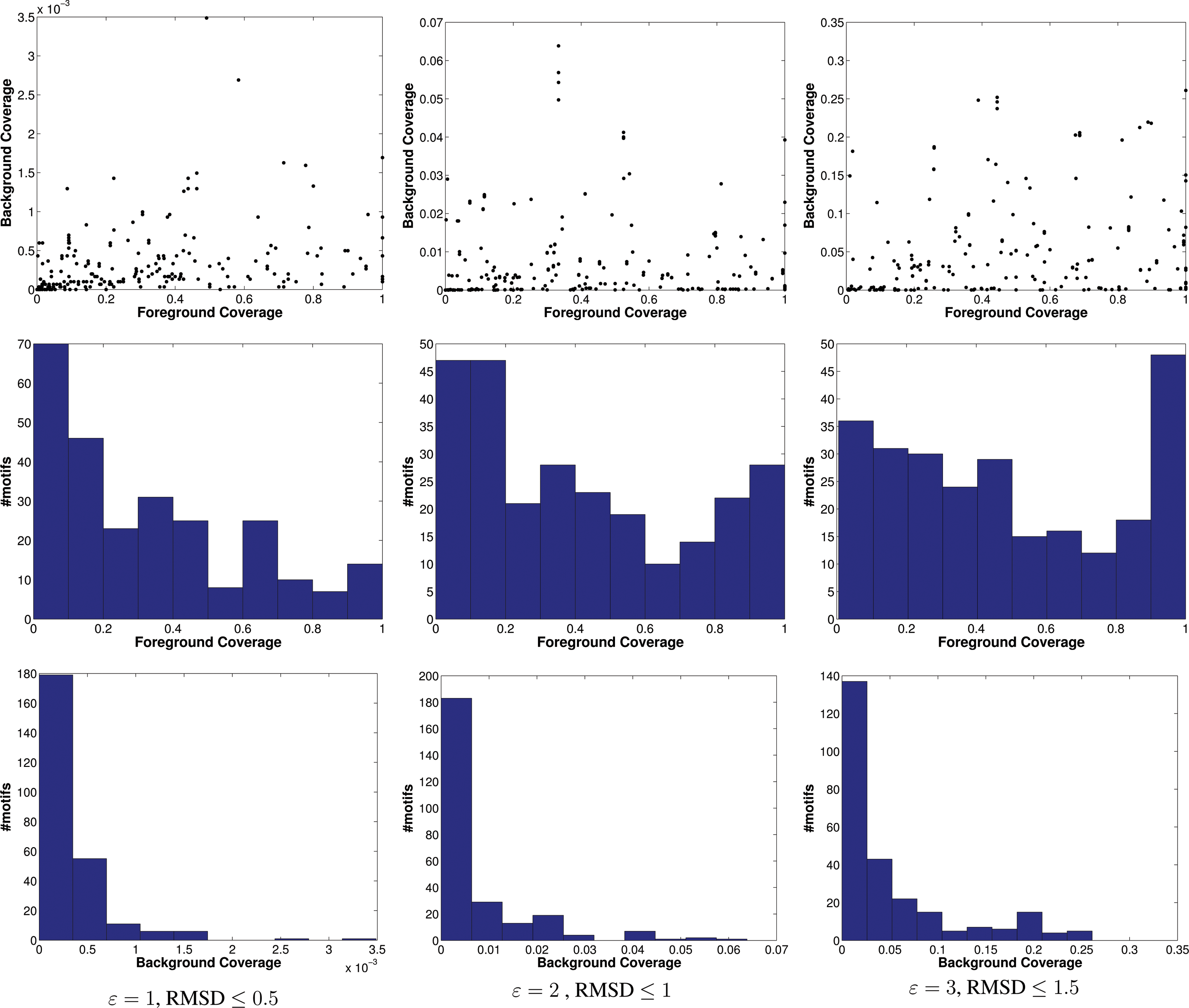
Unlike the enolase and SOIPPA-derived motifs, these are not rigorously defined or assessed as “motifs” per se, so they vary widely in their ability to capture the foreground and not the background. In fact, (Moll et al., 2010) found that while the motifs are quite specific, covering only 0.1–0.2% of the background, their sensitivity ranges from 0 to 100%. They discussed a number of reasons, including the fact that no amino acid substitutions were allowed, as well as the construction of the motifs based on CSA rather than EC classes. We found similar lack of specificity and sensitivity (Fig. 6 illustrates coverage of foreground and background by CSA motifs), but still use this dataset as a large-scale study of the effects of different motif definitions, with the number of points ranging from 4 to 8 and the radius from about 5 Å to about 37 Å [!].

FIG. 6.
Coverage of 147 CSA motifs, visualized as scatterplots (top panels); foreground histograms (middle panels); background histograms, at three different pairs of parameter settings (bottom panels).

Figure 4 (right panel) summarizes the wall-clock times required for background searches, aggregated by the radius, with different lines for different values of ɛ. The performance does depend on the motif radius, though the larger radii aren't really appropriate structural motifs. For motifs with a radius of at most 9 Å (in line with the case study motifs), the average running time was 600 seconds, while for larger motifs of radius 15 Å, it degraded smoothly to 1300 seconds. LabelHash did quite a bit better on these searches, averaging about 150 seconds for the (different) background search, since most of the motifs have a small number of points (4 or 5) and unique amino acid labels, so that indeed most of the effort is handled by hashing. We also aggregated the times by the number of points (Fig. 7 provides boxplots of CSA timing results at different values of ɛ). As we observed for SOIPPA motifs, Ballast is relatively insensitive to the number of motif points, in contrast to LabelHash and graph-based methods.

FIG. 7.
Wall-clock timing results for Ballast background searches. Boxplots over motifs in CSA database, grouped by number of points at different ɛ. Each box extends from the bottom quartile to the top one and whiskers extend 1.5 times this range.

4. Conclusion

We have presented a new approach to structural motif matching, making use of balls to localize computations, and directly utilizing both local geometry and chemical composition to find motif instances. We showed that our algorithm is efficient and effective in both theory and practice. Ballast's efficiency and its interpretable, tweakable parameters enable the analysis of structural variability inherent in the definition of a motif, and implications for specificity and sensitivity. It can thus also be quite useful in motif discovery. To a large extent, the Ballast approach is generic to assessments of geometric and compositional similarity, and while we instantiated it with common choices, it can readily support a variety of alternatives (distance difference, weighted metrics, solvent accessibility, local chemical environment). Ballast provides a powerful and efficient substrate for exploring fundamental questions in defining and developing motifs and characterizing sequence-structure-function relationships, and we look forward to further extending and applying it in a wide range of such contexts. A Java implementation of Ballast is freely available upon request.

Footnotes

Acknowledgment

This work was supported in part by NSF grant CCF-0915388 / 1023160, collaborative among CBK, GP, and FV.

Disclosure Statement

The authors declare that no competing financial interests exist.

1

We say that an event holds with high probability, abbreviated whp., if it holds with probability at least 1 − n^−c for some constant c > 0, for sufficiently large n.

References

Artymiuk

P.J.

, Poirrette

A.R.

, Grindley

H.M.

et al. 1994. A graph-theoretic approach to the identification of three-dimensional patterns of amino acid side-chains in protein structures. J. Mol. Biol., 243:327–344.

Arun

K.S.

, Huang

T.S.

, Blostein

S.D.

1987. Least-squares fitting of two 3-D point sets. IEEE Trans. Pattern Anal. Mach. Intell., 9:698–700.

Babbitt

P.C.

, Hasson

M.S.

, Wedekind

J.E.

et al. 1996. The enolase superfamily: A general strategy for enzyme-catalyzed abstraction of the α-protons of carboxylic acids. Biochemistry, 35:16489–16501.

Bandyopadhyay

, Snoeyink

2004. Almost-Delaunay simplices: nearest neighbor relations for imprecise points. Proc. SODA, 410–419.

Bandyopadhyay

, Huan

, Prins

et al. 2009. Identification of family-specific residue packing motifs and their use for structure-based protein function prediction: I. Method development. J. Comput. Aided Mol. Des., 23:773–784.

Barker

J.A.

, Thornton

J.M.

2003. An algorithm for constraint-based structural template matching: application to 3D templates with statistical analysis. Bioinformatics, 19:1644–1649.

Bernstein

F.C.

, Koetzle

T.F.

, Williams

G.J.

et al. 1977. The Protein Data Bank: a computer-based archival file for macromolecular structures. J. Mol. Biol., 112:535–542.

Bron

, Kerbosch

1973. Algorithm 457: finding all cliques of an undirected graph. Commun. ACM, 16:575–577.

Chen

B.Y.

, Fofanov

V.Y.

, Bryant

D.H.

et al. 2007. The MASH pipeline for protein function prediction and an algorithm for the geometric refinement of 3D motifs. J. Comput. Biol., 14:791–816.

10.

Feige

, Goldwasser

, Lovász

et al. 1996. Interactive proofs and the hardness of approximating cliques. J. ACM, 43:268–292.

11.

Gardiner

E.J.

, Artymiuk

P.J.

, Willett

. 1997. Clique-detection algorithms for matching three-dimensional molecular structures. J. Mol. Graph. Model., 15:245–253.

12.

Hegyi

, Gerstein

1999. The relationship between protein structure and function: a comprehensive survey with application to the yeast genome. J. Mol. Biol., 288:147–164.

13.

Karp

R.M.

1972. Reducibility among combinatorial problems. Complexity of Computer Computations, 40:85–103.

14.

Kleywegt

G.J.

1999. Recognition of spatial motifs in protein structures. J. Mol. Biol., 285:1887–1897.

15.

Loewenstein

, Raimondo

, Redfern

O.C.

et al. 2009. Protein function annotation by homology-based inference. Genome Biol., 10:207.

16.

Lueker

G.S.

1978. A data structure for orthogonal range queries. Proc. 19th Annual Symposium on Foundations of Computer Science, 28–34.

17.

Meng

E.C.

, Polacco

B.J

, Babbitt

P.C

. 2004. Superfamily active site templates. Proteins, 55:962–976.

18.

Milik

, Szalma

, Olszewski

K.A.

2003. Common Structural Cliques: a tool for protein structure and function analysis. Protein Eng., 16:543–552.

19.

Mitzenmacher

, Upfal

2005. Probability and Computing: Randomized Algorithms and Probabilistic Analysis. Cambridge Univ. Press: New York.

20.

Moll

, Bryant

D.H.

, Kavraki

L.E.

2010. The LabelHash algorithm for substructure matching. BMC Bioinformatics, 11:555.

21.

Muthukrishnan

, Pandurangan

2005. The bin-covering technique for thresholding random geometric graph properties. Proc. SODA, 989–998.

22.

Najmanovich

, Kurbatova

, Thornton

2008. Detection of 3D atomic similarities and their use in the discrimination of small molecule protein-binding sites. Bioinformatics, 24:i105–111.

23.

Nussinov

, Wolfson

H. J.

1991. Efficient detection of three-dimensional structural motifs in biological macromolecules by computer vision techniques. PNAS, 88:10495–10499.

24.

Pegg

S.C.

, Brown

S.D.

, Ojha

et al. 2006. Leveraging enzyme structure-function relationships for functional inference and experimental design: the structure-function linkage database. Biochemistry, 45:2545–2555.

25.

Penrose

M.D.

2003. Random Geometric Graphs. Oxford University Press: New York.

26.

Porter

C.T.

, Bartlett

G.J.

, Thornton

J.M.

2004. The Catalytic Site Atlas: a resource of catalytic sites and residues identified in enzymes using structural data. Nucleic Acids Res., 32:D129–133.

27.

Shulman-Peleg

, Nussinov

, Wolfson

H.J.

2004. Recognition of functional sites in protein structures. J. Mol. Biol., 339:607–633.

28.

Ullmann

J.R.

1976. An algorithm for subgraph isomorphism. J. ACM, 23:31–42.

29.

Wallace

A.C.

, Borkakoti

, Thornton

J.M.

1997. TESS: a geometric hashing algorithm for deriving 3D coordinate templates for searching structural databases. Application to enzyme active sites. Protein Sci., 6:2308–2323.

30.

Wangikar

P.P.

, Tendulkar

A.V.

, Ramya

et al. 2003. Functional sites in protein families uncovered via an objective and automated graph theoretic approach. J. Mol. Biol., 326:955–978.

31.

Willard

D.E.

1978. Predicate-Oriented Database Search Algorithms. Outstanding Dissertations in the Computer Sciences. Garland Publishing: New York.

32.

Wolfson

H.J.

, Rigoutsos

1997. Geometric hashing: An overview. Computing in Science and Engineering, 4:10–21.

33.

Xie

, Bourne

P.E.

2008. Detecting evolutionary relationships across existing fold space, using sequence order-independent profile-profile alignments. PNAS, 105:5441–5446.