An Effective Exact Algorithm and a New Upper Bound for the Number of Contacts in the Hydrophobic-Polar Two-Dimensional Lattice Model

2.1. Preliminary definitions

Let Σ be a finite alphabet of symbols and Σ* the Kleene star of Σ, that is, the set of all possible finite sequences of symbols belonging to Σ. An amino acid sequence of length n is a sequence \documentclass{aastex}\usepackage{amsbsy}\usepackage{amsfonts}\usepackage{amssymb}\usepackage{bm}\usepackage{mathrsfs}\usepackage{pifont}\usepackage{stmaryrd}\usepackage{textcomp}\usepackage{portland, xspace}\usepackage{amsmath, amsxtra}\pagestyle{empty}\DeclareMathSizes{10}{9}{7}{6}\begin{document} $$a_1 , \ldots , a_n \in (\{A , \ldots , Z \} \setminus \{B , J , O , U , X , Z \}) ^*$$ \end{document} . The HP encoding of an amino acid sequence \documentclass{aastex}\usepackage{amsbsy}\usepackage{amsfonts}\usepackage{amssymb}\usepackage{bm}\usepackage{mathrsfs}\usepackage{pifont}\usepackage{stmaryrd}\usepackage{textcomp}\usepackage{portland, xspace}\usepackage{amsmath, amsxtra}\pagestyle{empty}\DeclareMathSizes{10}{9}{7}{6}\begin{document} $$a_1 , \ldots , a_n$$ \end{document} is the sequence \documentclass{aastex}\usepackage{amsbsy}\usepackage{amsfonts}\usepackage{amssymb}\usepackage{bm}\usepackage{mathrsfs}\usepackage{pifont}\usepackage{stmaryrd}\usepackage{textcomp}\usepackage{portland, xspace}\usepackage{amsmath, amsxtra}\pagestyle{empty}\DeclareMathSizes{10}{9}{7}{6}\begin{document} $$\hat{a}_1 , \ldots , \hat{a}_n \in \{H , P \} ^*$$ \end{document} , where \documentclass{aastex}\usepackage{amsbsy}\usepackage{amsfonts}\usepackage{amssymb}\usepackage{bm}\usepackage{mathrsfs}\usepackage{pifont}\usepackage{stmaryrd}\usepackage{textcomp}\usepackage{portland, xspace}\usepackage{amsmath, amsxtra}\pagestyle{empty}\DeclareMathSizes{10}{9}{7}{6}\begin{document} \begin{align*}\hat{a}_i = \begin{cases}H \qquad {\rm if} \ a_i \in \{A , V , L , I , P , F , M , W , G , C \} \\ P \qquad{\rm otherwise}\end{cases}\end{align*} \end{document}

for \documentclass{aastex}\usepackage{amsbsy}\usepackage{amsfonts}\usepackage{amssymb}\usepackage{bm}\usepackage{mathrsfs}\usepackage{pifont}\usepackage{stmaryrd}\usepackage{textcomp}\usepackage{portland, xspace}\usepackage{amsmath, amsxtra}\pagestyle{empty}\DeclareMathSizes{10}{9}{7}{6}\begin{document} $$i = 1 , \ldots , n$$ \end{document} . We encode a self-avoiding walk on a 2D lattice of an HP sequence \documentclass{aastex}\usepackage{amsbsy}\usepackage{amsfonts}\usepackage{amssymb}\usepackage{bm}\usepackage{mathrsfs}\usepackage{pifont}\usepackage{stmaryrd}\usepackage{textcomp}\usepackage{portland, xspace}\usepackage{amsmath, amsxtra}\pagestyle{empty}\DeclareMathSizes{10}{9}{7}{6}\begin{document} $$\hat{a}_1 , \ldots , \hat{a}_n$$ \end{document} as the sequence \documentclass{aastex}\usepackage{amsbsy}\usepackage{amsfonts}\usepackage{amssymb}\usepackage{bm}\usepackage{mathrsfs}\usepackage{pifont}\usepackage{stmaryrd}\usepackage{textcomp}\usepackage{portland, xspace}\usepackage{amsmath, amsxtra}\pagestyle{empty}\DeclareMathSizes{10}{9}{7}{6}\begin{document} $$\langle d_1 , \ldots , d_{n - 1} \rangle$$ \end{document} , where \documentclass{aastex}\usepackage{amsbsy}\usepackage{amsfonts}\usepackage{amssymb}\usepackage{bm}\usepackage{mathrsfs}\usepackage{pifont}\usepackage{stmaryrd}\usepackage{textcomp}\usepackage{portland, xspace}\usepackage{amsmath, amsxtra}\pagestyle{empty}\DeclareMathSizes{10}{9}{7}{6}\begin{document} $$d_i \in \{L , R , U , D \} $$ \end{document} is the direction of the link that connects beads â_i and â_i+1. Observe that, for i ≥ 2, each d_i can be chosen in at most three ways, because there are at most three empty cells that are first-neighbors to bead â_i-1. Moreover, the second bead, and its associated direction d₁, can be fixed at any of the four first-neighbor sites that are all equivalent by symmetry. Given a configuration \documentclass{aastex}\usepackage{amsbsy}\usepackage{amsfonts}\usepackage{amssymb}\usepackage{bm}\usepackage{mathrsfs}\usepackage{pifont}\usepackage{stmaryrd}\usepackage{textcomp}\usepackage{portland, xspace}\usepackage{amsmath, amsxtra}\pagestyle{empty}\DeclareMathSizes{10}{9}{7}{6}\begin{document} $$\langle d_1 , \ldots , d_{n - 1} \rangle$$ \end{document} , we define the vector (x_i, y_i) as the coordinate of bead â_i in the lattice, where \documentclass{aastex}\usepackage{amsbsy}\usepackage{amsfonts}\usepackage{amssymb}\usepackage{bm}\usepackage{mathrsfs}\usepackage{pifont}\usepackage{stmaryrd}\usepackage{textcomp}\usepackage{portland, xspace}\usepackage{amsmath, amsxtra}\pagestyle{empty}\DeclareMathSizes{10}{9}{7}{6}\begin{document} \begin{align*}(x_i , y_i) = \begin{cases}(0 , 0) \quad\quad\quad\quad\quad {\rm if} \ i = 1 \\ (x_{i - 1} - 1 , y_{i - 1}) \ {\rm if} \ i > 1 \ {\rm and} \ d_{i - 1} = L \\ (x_{i - 1} + 1 , y_{i - 1}) \ {\rm if} \ i > 1 \ {\rm and} \ d_{i - 1} = R \\ (x_{i - 1} , y_{i - 1} - 1) \ {\rm if} \ i > 1 \ {\rm and } \ d_{i - 1} = U \\ (x_{i - 1} , y_{i - 1} + 1) \ {\rm if} \ i > 1 \ {\rm and} \ d_{i - 1} = D \end{cases}\end{align*} \end{document}

Given two distinct beads â_i and â_j, i ≠ j, we define the energy of the corresponding contact, if any, as ε(i, j) = C(i, j)E(â_i,â _j), where \documentclass{aastex}\usepackage{amsbsy}\usepackage{amsfonts}\usepackage{amssymb}\usepackage{bm}\usepackage{mathrsfs}\usepackage{pifont}\usepackage{stmaryrd}\usepackage{textcomp}\usepackage{portland, xspace}\usepackage{amsmath, amsxtra}\pagestyle{empty}\DeclareMathSizes{10}{9}{7}{6}\begin{document} \begin{align*}C (i , j) = \begin{cases}1 \qquad {\rm if} \ \mid i - j \mid \neq 1 \ {\rm and} \ d ((x_i , y_i) , (x_j , y_j)) = 1 \\ 0 \qquad {\rm otherwise}\end{cases}\end{align*} \end{document}

indicates whether the beads are topologically first-neighbors (d(·) is the euclidean distance) and are not adjacent in the original sequence and \documentclass{aastex}\usepackage{amsbsy}\usepackage{amsfonts}\usepackage{amssymb}\usepackage{bm}\usepackage{mathrsfs}\usepackage{pifont}\usepackage{stmaryrd}\usepackage{textcomp}\usepackage{portland, xspace}\usepackage{amsmath, amsxtra}\pagestyle{empty}\DeclareMathSizes{10}{9}{7}{6}\begin{document} \begin{align*}E (\hat{a}_1 , \hat{a}_2) = \begin{cases} - 1 \ \quad {\rm if} \ \hat{a}_1 = \hat{a}_2 = H \\ 0 \qquad {\rm otherwise}\end{cases}\end{align*} \end{document}

defines the energy of a contact depending on the bead types. In the HP model, an HH contact provides a unitary contribution while all the other combinations yield zero energy. Finally, we define the energy of a configuration as \documentclass{aastex}\usepackage{amsbsy}\usepackage{amsfonts}\usepackage{amssymb}\usepackage{bm}\usepackage{mathrsfs}\usepackage{pifont}\usepackage{stmaryrd}\usepackage{textcomp}\usepackage{portland, xspace}\usepackage{amsmath, amsxtra}\pagestyle{empty}\DeclareMathSizes{10}{9}{7}{6}\begin{document} \begin{align*}\sum_{i < j} \epsilon (i , j)\end{align*} \end{document}

In this model, the problem of finding the configuration(s) with minimal energy is equivalent to finding the configuration(s) with maximum number of HH contacts.

Given an HP sequence \documentclass{aastex}\usepackage{amsbsy}\usepackage{amsfonts}\usepackage{amssymb}\usepackage{bm}\usepackage{mathrsfs}\usepackage{pifont}\usepackage{stmaryrd}\usepackage{textcomp}\usepackage{portland, xspace}\usepackage{amsmath, amsxtra}\pagestyle{empty}\DeclareMathSizes{10}{9}{7}{6}\begin{document} $$S = \hat{a}_1 , \ldots , \hat{a}_n$$ \end{document} , we partition the set of H beads into the following two subsets: \documentclass{aastex}\usepackage{amsbsy}\usepackage{amsfonts}\usepackage{amssymb}\usepackage{bm}\usepackage{mathrsfs}\usepackage{pifont}\usepackage{stmaryrd}\usepackage{textcomp}\usepackage{portland, xspace}\usepackage{amsmath, amsxtra}\pagestyle{empty}\DeclareMathSizes{10}{9}{7}{6}\begin{document} \begin{align*} & {\cal H}_E = \{i \mid \hat{a}_i = H \ {\rm and} \ i \ {\rm mod} \ 2 = 0 \} \\ & {\cal H}_O = \{i \mid \hat{a}_i = H \ {\rm and} \ i \ {\rm mod} \ 2 = 1 \} \end{align*} \end{document}

We say that an H bead is of type E(O) if it belongs to the subset \documentclass{aastex}\usepackage{amsbsy}\usepackage{amsfonts}\usepackage{amssymb}\usepackage{bm}\usepackage{mathrsfs}\usepackage{pifont}\usepackage{stmaryrd}\usepackage{textcomp}\usepackage{portland, xspace}\usepackage{amsmath, amsxtra}\pagestyle{empty}\DeclareMathSizes{10}{9}{7}{6}\begin{document} $${\cal H}_E ({\cal H}_O)$$ \end{document} . The \documentclass{aastex}\usepackage{amsbsy}\usepackage{amsfonts}\usepackage{amssymb}\usepackage{bm}\usepackage{mathrsfs}\usepackage{pifont}\usepackage{stmaryrd}\usepackage{textcomp}\usepackage{portland, xspace}\usepackage{amsmath, amsxtra}\pagestyle{empty}\DeclareMathSizes{10}{9}{7}{6}\begin{document} $${\cal H}_E$$ \end{document} set contains all H beads of even index, and the \documentclass{aastex}\usepackage{amsbsy}\usepackage{amsfonts}\usepackage{amssymb}\usepackage{bm}\usepackage{mathrsfs}\usepackage{pifont}\usepackage{stmaryrd}\usepackage{textcomp}\usepackage{portland, xspace}\usepackage{amsmath, amsxtra}\pagestyle{empty}\DeclareMathSizes{10}{9}{7}{6}\begin{document} $${\cal H}_O$$ \end{document} set contains all H beads of odd index. It is easy to see that on a 2D lattice an HH contact is possible only between two beads that do not belong to the same subset, as no pair of beads in either subset can be first-neighbors. This property is known as the parity problem and holds also in cubic lattices. Given a bead â_i, for \documentclass{aastex}\usepackage{amsbsy}\usepackage{amsfonts}\usepackage{amssymb}\usepackage{bm}\usepackage{mathrsfs}\usepackage{pifont}\usepackage{stmaryrd}\usepackage{textcomp}\usepackage{portland, xspace}\usepackage{amsmath, amsxtra}\pagestyle{empty}\DeclareMathSizes{10}{9}{7}{6}\begin{document} $$i = 1 , \ldots , n$$ \end{document} , we say that the bead is internal if \documentclass{aastex}\usepackage{amsbsy}\usepackage{amsfonts}\usepackage{amssymb}\usepackage{bm}\usepackage{mathrsfs}\usepackage{pifont}\usepackage{stmaryrd}\usepackage{textcomp}\usepackage{portland, xspace}\usepackage{amsmath, amsxtra}\pagestyle{empty}\DeclareMathSizes{10}{9}{7}{6}\begin{document} $$i\, {\notin} \{1 , n \} $$ \end{document} . Note that, in any configuration that is a valid self-avoiding walk, all internal beads have exactly two sequence-adjacent elements, while the first and the last bead have exactly one sequence-adjacent element. The following elementary lemma holds:

Lemma 1. Given an HP sequence of length n, the maximum number of nonadjacent first neighbors of a given bead, in any self-avoiding walk covering the whole sequence, is equal to 2 if the bead is internal and to 3 otherwise, that is, \documentclass{aastex}\usepackage{amsbsy}\usepackage{amsfonts}\usepackage{amssymb}\usepackage{bm}\usepackage{mathrsfs}\usepackage{pifont}\usepackage{stmaryrd}\usepackage{textcomp}\usepackage{portland, xspace}\usepackage{amsmath, amsxtra}\pagestyle{empty}\DeclareMathSizes{10}{9}{7}{6}\begin{document} \begin{align*}\sum_j C (i , j) \le \begin{cases}2 \qquad if \ i\ \notin\ \{1 , n \} \\ 3 \qquad otherwise\end{cases}\end{align*} \end{document}

for all i = 1, … ,n.

Hence, the maximum number of contacts in which a bead can participate is equal to 2 if the bead is internal and to 3 otherwise. The maximum number of contacts achievable by the beads of type O and E is then \documentclass{aastex}\usepackage{amsbsy}\usepackage{amsfonts}\usepackage{amssymb}\usepackage{bm}\usepackage{mathrsfs}\usepackage{pifont}\usepackage{stmaryrd}\usepackage{textcomp}\usepackage{portland, xspace}\usepackage{amsmath, amsxtra}\pagestyle{empty}\DeclareMathSizes{10}{9}{7}{6}\begin{document} \begin{align*} \begin{split} & C_E = 2 \mid {\cal H}_E \mid + e_E \\ & C_O = 2 \mid {\cal H}_O \mid + e_1 + e_O\end{split} \tag{1}\end{align*} \end{document}

where the e_x terms take care to consider extra contacts made by sequence extremities: e_E is 1 if \documentclass{aastex}\usepackage{amsbsy}\usepackage{amsfonts}\usepackage{amssymb}\usepackage{bm}\usepackage{mathrsfs}\usepackage{pifont}\usepackage{stmaryrd}\usepackage{textcomp}\usepackage{portland, xspace}\usepackage{amsmath, amsxtra}\pagestyle{empty}\DeclareMathSizes{10}{9}{7}{6}\begin{document} $$\hat{a}_n \in {\cal H}_E$$ \end{document} and 0 otherwise, e_O is defined analogously to e_E, and e₁ is 1 if â₁ = H and 0 otherwise. The maximum number of contacts achievable by the HP sequence S is then bounded with the number \documentclass{aastex}\usepackage{amsbsy}\usepackage{amsfonts}\usepackage{amssymb}\usepackage{bm}\usepackage{mathrsfs}\usepackage{pifont}\usepackage{stmaryrd}\usepackage{textcomp}\usepackage{portland, xspace}\usepackage{amsmath, amsxtra}\pagestyle{empty}\DeclareMathSizes{10}{9}{7}{6}\begin{document} \begin{align*}C_{\rm parity} = \min (C_E , C_O) \tag{2}\end{align*} \end{document}

However, in the next section we present a new upper bound on the number of contacts achievable by an HP sequence.

2.2. New results on the structures of HP sequences

In this section, we present some new results on the configurations of HP sequences on the 2D lattice model. Given a configuration of an HP sequence on a 2D lattice, we define the H-core as the smallest rectangle containing all the H beads. Let \documentclass{aastex}\usepackage{amsbsy}\usepackage{amsfonts}\usepackage{amssymb}\usepackage{bm}\usepackage{mathrsfs}\usepackage{pifont}\usepackage{stmaryrd}\usepackage{textcomp}\usepackage{portland, xspace}\usepackage{amsmath, amsxtra}\pagestyle{empty}\DeclareMathSizes{10}{9}{7}{6}\begin{document} $$S = \hat{a}_1 , \ldots , \hat{a}_n$$ \end{document} be an HP sequence with m H beads and let also \documentclass{aastex}\usepackage{amsbsy}\usepackage{amsfonts}\usepackage{amssymb}\usepackage{bm}\usepackage{mathrsfs}\usepackage{pifont}\usepackage{stmaryrd}\usepackage{textcomp}\usepackage{portland, xspace}\usepackage{amsmath, amsxtra}\pagestyle{empty}\DeclareMathSizes{10}{9}{7}{6}\begin{document} \begin{align*}{\cal P}_S = \{i \mid 2 \le i < n \wedge \hat{a}_i = P \wedge \hat{a}_{i - 1} = \hat{a}_{i + 1} = H \} \end{align*} \end{document}

be the set of P beads whose previous and next neighbors in the sequence are H beads. We call such beads P singlets. Observe that the minimum area that the H-core must span is equal to \documentclass{aastex}\usepackage{amsbsy}\usepackage{amsfonts}\usepackage{amssymb}\usepackage{bm}\usepackage{mathrsfs}\usepackage{pifont}\usepackage{stmaryrd}\usepackage{textcomp}\usepackage{portland, xspace}\usepackage{amsmath, amsxtra}\pagestyle{empty}\DeclareMathSizes{10}{9}{7}{6}\begin{document} \begin{align*}A_{\min} = m + \mid {\cal P}_S \mid\end{align*} \end{document}

because it must contain, by definition, all the H beads, as well as all the P beads in \documentclass{aastex}\usepackage{amsbsy}\usepackage{amsfonts}\usepackage{amssymb}\usepackage{bm}\usepackage{mathrsfs}\usepackage{pifont}\usepackage{stmaryrd}\usepackage{textcomp}\usepackage{portland, xspace}\usepackage{amsmath, amsxtra}\pagestyle{empty}\DeclareMathSizes{10}{9}{7}{6}\begin{document} $${\cal P}_S$$ \end{document} , since it is not possible to place them outside the core.

We now introduce the concept of a connected H-core, which in turn will lead to the definition of a new upper bound on the number of contacts achievable by an HP sequence. We say that an H-core is connected if it satisfies the property that each row and column contains at least one H bead or one P singlet. We devise an interesting relationship between the size of a connected H-core and the maximum number of contacts that can be achieved within it. Let (L₁,L₂) be the dimensions of an H-core. The number of cells available in such a rectangle is L₁L₂ and the number of segments in such a rectangle, which represents the maximum number of contacts that can be obtained by placing an H bead in each cell, is \documentclass{aastex}\usepackage{amsbsy}\usepackage{amsfonts}\usepackage{amssymb}\usepackage{bm}\usepackage{mathrsfs}\usepackage{pifont}\usepackage{stmaryrd}\usepackage{textcomp}\usepackage{portland, xspace}\usepackage{amsmath, amsxtra}\pagestyle{empty}\DeclareMathSizes{10}{9}{7}{6}\begin{document} \begin{align*}(L_1 - 1) L_2 + (L_2 - 1) L_1.\end{align*} \end{document}

This can be observed in Figure 1a, depicting an example H-core of dimensions L₁ = 3 and L₂ = 4, correspondingly containing 12 cells (3 * 4) and 17 segments (2 * 4 + 3 * 3) linking these cells. These segments represent the potential contacts that a given configuration, within such H-core, can realize.

OPEN IN VIEWER

FIG. 1.

(a) Number of cells and segments for an H-core of dimensions L₁ = 3 and L₂ = 4. (b) A configuration for sequence HHHPHHHHPHP. (c) Analysis of such configuration, in terms of segment types: 4 segments are realized into contacts, 5 are internal H-H links, and 8 segments are wasted. (d) A different configuration for the same sequence. (e) Analysis of such configuration (now only 1 contact is realized, and 11 are wasted).

Observe that in an H-core with dimensions (L₁, L₂), m cells will be occupied by H beads, and therefore L₁L₂ −m cells must be either empty or occupied with P beads. The segments adjacent to these cells cannot contribute any contact. Figure 1b shows a sequence (HHHPHHHHPHP) configured into the example H-core; and for such configuration, Figure 1c analyzes the nature of the available 17 segments. Four (in red) are realized into contacts, while the remaining 13 are not. Of the remaining 13: five (in black) are H-H links internal to the sequence, and eight (in light gray) are adjacent to non–H-cell segments. We call these “wasted.” Figure 1d and e show a different configuration for the same sequence, which realizes only one contact: for the remaining segments, five are H-H links internal to the sequence (this number is of course a property of the sequence and does not depend on the configuration) and as many as 11 segments are wasted.

In order to estimate the minimum number of segments that must be wasted (i.e., they are not realized into contacts) because of non–H-cells, we introduce the following simple result:

Lemma 2. Let \documentclass{aastex}\usepackage{amsbsy}\usepackage{amsfonts}\usepackage{amssymb}\usepackage{bm}\usepackage{mathrsfs}\usepackage{pifont}\usepackage{stmaryrd}\usepackage{textcomp}\usepackage{portland, xspace}\usepackage{amsmath, amsxtra}\pagestyle{empty}\DeclareMathSizes{10}{9}{7}{6}\begin{document} $$\bar{P}$$ \end{document} denote either a P bead or an empty cell on the lattice. Given an H-core and an associated row (column) with \documentclass{aastex}\usepackage{amsbsy}\usepackage{amsfonts}\usepackage{amssymb}\usepackage{bm}\usepackage{mathrsfs}\usepackage{pifont}\usepackage{stmaryrd}\usepackage{textcomp}\usepackage{portland, xspace}\usepackage{amsmath, amsxtra}\pagestyle{empty}\DeclareMathSizes{10}{9}{7}{6}\begin{document} $$n_{\bar{P}} > {\ 0}$$ \end{document} beads of type \documentclass{aastex}\usepackage{amsbsy}\usepackage{amsfonts}\usepackage{amssymb}\usepackage{bm}\usepackage{mathrsfs}\usepackage{pifont}\usepackage{stmaryrd}\usepackage{textcomp}\usepackage{portland, xspace}\usepackage{amsmath, amsxtra}\pagestyle{empty}\DeclareMathSizes{10}{9}{7}{6}\begin{document} $$\bar{P}$$ \end{document} , the number of \documentclass{aastex}\usepackage{amsbsy}\usepackage{amsfonts}\usepackage{amssymb}\usepackage{bm}\usepackage{mathrsfs}\usepackage{pifont}\usepackage{stmaryrd}\usepackage{textcomp}\usepackage{portland, xspace}\usepackage{amsmath, amsxtra}\pagestyle{empty}\DeclareMathSizes{10}{9}{7}{6}\begin{document} $$H \bar{P}$$ \end{document} and \documentclass{aastex}\usepackage{amsbsy}\usepackage{amsfonts}\usepackage{amssymb}\usepackage{bm}\usepackage{mathrsfs}\usepackage{pifont}\usepackage{stmaryrd}\usepackage{textcomp}\usepackage{portland, xspace}\usepackage{amsmath, amsxtra}\pagestyle{empty}\DeclareMathSizes{10}{9}{7}{6}\begin{document} $$\bar{P} \bar{P}$$ \end{document} pairs of adjacent beads in the row (column) is equal to \documentclass{aastex}\usepackage{amsbsy}\usepackage{amsfonts}\usepackage{amssymb}\usepackage{bm}\usepackage{mathrsfs}\usepackage{pifont}\usepackage{stmaryrd}\usepackage{textcomp}\usepackage{portland, xspace}\usepackage{amsmath, amsxtra}\pagestyle{empty}\DeclareMathSizes{10}{9}{7}{6}\begin{document} $$n_{\bar {P}} - 1 + n_H$$ \end{document} , where n_H is the number of H beads after collapsing all the sequences of adjacent H beads into a single H bead.

Proof. Consider the row (column) obtained by collapsing all the sequences of adjacent H beads into a single H bead; this normalization removes all the HH pairs, making the analysis simpler, and does not change the number of \documentclass{aastex}\usepackage{amsbsy}\usepackage{amsfonts}\usepackage{amssymb}\usepackage{bm}\usepackage{mathrsfs}\usepackage{pifont}\usepackage{stmaryrd}\usepackage{textcomp}\usepackage{portland, xspace}\usepackage{amsmath, amsxtra}\pagestyle{empty}\DeclareMathSizes{10}{9}{7}{6}\begin{document} $${\bar{\rm P}} \bar{\rm P}$$ \end{document} and \documentclass{aastex}\usepackage{amsbsy}\usepackage{amsfonts}\usepackage{amssymb}\usepackage{bm}\usepackage{mathrsfs}\usepackage{pifont}\usepackage{stmaryrd}\usepackage{textcomp}\usepackage{portland, xspace}\usepackage{amsmath, amsxtra}\pagestyle{empty}\DeclareMathSizes{10}{9}{7}{6}\begin{document} $$\hbox{H}\bar{\rm P}$$ \end{document} pairs. Let h_e be the number of H beads that are adjacent, in the normalized sequence, to one \documentclass{aastex}\usepackage{amsbsy}\usepackage{amsfonts}\usepackage{amssymb}\usepackage{bm}\usepackage{mathrsfs}\usepackage{pifont}\usepackage{stmaryrd}\usepackage{textcomp}\usepackage{portland, xspace}\usepackage{amsmath, amsxtra}\pagestyle{empty}\DeclareMathSizes{10}{9}{7}{6}\begin{document} $$\bar{\rm P}$$ \end{document} bead, that is, the number of H beads that are the first or last element of the row (column); n_H−h_e is thus the number of H beads that are adjacent to two \documentclass{aastex}\usepackage{amsbsy}\usepackage{amsfonts}\usepackage{amssymb}\usepackage{bm}\usepackage{mathrsfs}\usepackage{pifont}\usepackage{stmaryrd}\usepackage{textcomp}\usepackage{portland, xspace}\usepackage{amsmath, amsxtra}\pagestyle{empty}\DeclareMathSizes{10}{9}{7}{6}\begin{document} $$\bar{\rm P}$$ \end{document} beads. Then, it is easy to verify that the number of \documentclass{aastex}\usepackage{amsbsy}\usepackage{amsfonts}\usepackage{amssymb}\usepackage{bm}\usepackage{mathrsfs}\usepackage{pifont}\usepackage{stmaryrd}\usepackage{textcomp}\usepackage{portland, xspace}\usepackage{amsmath, amsxtra}\pagestyle{empty}\DeclareMathSizes{10}{9}{7}{6}\begin{document} $$\bar{\rm P} \bar{\rm P}$$ \end{document} and \documentclass{aastex}\usepackage{amsbsy}\usepackage{amsfonts}\usepackage{amssymb}\usepackage{bm}\usepackage{mathrsfs}\usepackage{pifont}\usepackage{stmaryrd}\usepackage{textcomp}\usepackage{portland, xspace}\usepackage{amsmath, amsxtra}\pagestyle{empty}\DeclareMathSizes{10}{9}{7}{6}\begin{document} $${\rm H} \bar{\rm P}$$ \end{document} pairs is equal to \documentclass{aastex}\usepackage{amsbsy}\usepackage{amsfonts}\usepackage{amssymb}\usepackage{bm}\usepackage{mathrsfs}\usepackage{pifont}\usepackage{stmaryrd}\usepackage{textcomp}\usepackage{portland, xspace}\usepackage{amsmath, amsxtra}\pagestyle{empty}\DeclareMathSizes{10}{9}{7}{6}\begin{document} $$n_{\bar{P}} - 1 - (n_H - h_e)$$ \end{document} and 2(n_H−h_e) + h_e, respectively. Hence, the total number of pairs is \documentclass{aastex}\usepackage{amsbsy}\usepackage{amsfonts}\usepackage{amssymb}\usepackage{bm}\usepackage{mathrsfs}\usepackage{pifont}\usepackage{stmaryrd}\usepackage{textcomp}\usepackage{portland, xspace}\usepackage{amsmath, amsxtra}\pagestyle{empty}\DeclareMathSizes{10}{9}{7}{6}\begin{document} $$n_{\bar{P}} - 1 + n_H$$ \end{document} and the claim follows.

Let \documentclass{aastex}\usepackage{amsbsy}\usepackage{amsfonts}\usepackage{amssymb}\usepackage{bm}\usepackage{mathrsfs}\usepackage{pifont}\usepackage{stmaryrd}\usepackage{textcomp}\usepackage{portland, xspace}\usepackage{amsmath, amsxtra}\pagestyle{empty}\DeclareMathSizes{10}{9}{7}{6}\begin{document} $$n_{\bar{P}} (i , *)$$ \end{document} and \documentclass{aastex}\usepackage{amsbsy}\usepackage{amsfonts}\usepackage{amssymb}\usepackage{bm}\usepackage{mathrsfs}\usepackage{pifont}\usepackage{stmaryrd}\usepackage{textcomp}\usepackage{portland, xspace}\usepackage{amsmath, amsxtra}\pagestyle{empty}\DeclareMathSizes{10}{9}{7}{6}\begin{document} $$n_{\bar{P}} (* , \ j)$$ \end{document} denote the number of beads of type \documentclass{aastex}\usepackage{amsbsy}\usepackage{amsfonts}\usepackage{amssymb}\usepackage{bm}\usepackage{mathrsfs}\usepackage{pifont}\usepackage{stmaryrd}\usepackage{textcomp}\usepackage{portland, xspace}\usepackage{amsmath, amsxtra}\pagestyle{empty}\DeclareMathSizes{10}{9}{7}{6}\begin{document} $$\bar{\rm P}$$ \end{document} in the i-th row and in the j-th column, respectively; likewise for n_H(i,* ) and n_H(*, j). Let also \documentclass{aastex}\usepackage{amsbsy}\usepackage{amsfonts}\usepackage{amssymb}\usepackage{bm}\usepackage{mathrsfs}\usepackage{pifont}\usepackage{stmaryrd}\usepackage{textcomp}\usepackage{portland, xspace}\usepackage{amsmath, amsxtra}\pagestyle{empty}\DeclareMathSizes{10}{9}{7}{6}\begin{document} $$R_P = \{1 \le i \le L_1 \mid n_{\bar{P}} (i , *) > 0 \} $$ \end{document} and \documentclass{aastex}\usepackage{amsbsy}\usepackage{amsfonts}\usepackage{amssymb}\usepackage{bm}\usepackage{mathrsfs}\usepackage{pifont}\usepackage{stmaryrd}\usepackage{textcomp}\usepackage{portland, xspace}\usepackage{amsmath, amsxtra}\pagestyle{empty}\DeclareMathSizes{10}{9}{7}{6}\begin{document} $$C_P = \{1 \le j \le L_2 \mid n_{\bar{P}} (* ,\ j) > 0 \} $$ \end{document} be the set of row and column indexes with at least one P bead. Based on Lemma 2, we are now able to provide a lower bound on the number of wasted contacts in a connected H-core:

Theorem 1. Given a connected H-core with dimensions (L₁, L₂) and containing m H beads, the number of \documentclass{aastex}\usepackage{amsbsy}\usepackage{amsfonts}\usepackage{amssymb}\usepackage{bm}\usepackage{mathrsfs}\usepackage{pifont}\usepackage{stmaryrd}\usepackage{textcomp}\usepackage{portland, xspace}\usepackage{amsmath, amsxtra}\pagestyle{empty}\DeclareMathSizes{10}{9}{7}{6}\begin{document} $${\rm H} \bar{\rm P}$$ \end{document} and \documentclass{aastex}\usepackage{amsbsy}\usepackage{amsfonts}\usepackage{amssymb}\usepackage{bm}\usepackage{mathrsfs}\usepackage{pifont}\usepackage{stmaryrd}\usepackage{textcomp}\usepackage{portland, xspace}\usepackage{amsmath, amsxtra}\pagestyle{empty}\DeclareMathSizes{10}{9}{7}{6}\begin{document} $$\bar{\rm P} \bar{\rm P}$$ \end{document} pairs is at least 2(L₁L₂ −m).

Proof. By Lemma 2, the total number of \documentclass{aastex}\usepackage{amsbsy}\usepackage{amsfonts}\usepackage{amssymb}\usepackage{bm}\usepackage{mathrsfs}\usepackage{pifont}\usepackage{stmaryrd}\usepackage{textcomp}\usepackage{portland, xspace}\usepackage{amsmath, amsxtra}\pagestyle{empty}\DeclareMathSizes{10}{9}{7}{6}\begin{document} $${\rm H} \bar{\rm P}$$ \end{document} and \documentclass{aastex}\usepackage{amsbsy}\usepackage{amsfonts}\usepackage{amssymb}\usepackage{bm}\usepackage{mathrsfs}\usepackage{pifont}\usepackage{stmaryrd}\usepackage{textcomp}\usepackage{portland, xspace}\usepackage{amsmath, amsxtra}\pagestyle{empty}\DeclareMathSizes{10}{9}{7}{6}\begin{document} $$\bar{\rm P} \bar{\rm P}$$ \end{document} pairs is equal to \documentclass{aastex}\usepackage{amsbsy}\usepackage{amsfonts}\usepackage{amssymb}\usepackage{bm}\usepackage{mathrsfs}\usepackage{pifont}\usepackage{stmaryrd}\usepackage{textcomp}\usepackage{portland, xspace}\usepackage{amsmath, amsxtra}\pagestyle{empty}\DeclareMathSizes{10}{9}{7}{6}\begin{document} \begin{align*}\sum_{i \in R_P} n_{\bar{P}} (i , *) + \sum_{j \in C_P} n_{\bar{P}} (* ,\ j) + \sum_{i \in R_P} (n_H (i , *) - 1) + \sum_{j \in C_P} (n_H (* ,\ j) - 1) .\end{align*} \end{document}

It is easy to see that the first part of the expression, \documentclass{aastex}\usepackage{amsbsy}\usepackage{amsfonts}\usepackage{amssymb}\usepackage{bm}\usepackage{mathrsfs}\usepackage{pifont}\usepackage{stmaryrd}\usepackage{textcomp}\usepackage{portland, xspace}\usepackage{amsmath, amsxtra}\pagestyle{empty}\DeclareMathSizes{10}{9}{7}{6}\begin{document} $$\sum_{i \in R_P} n_{\bar{P}} (i , *) + \sum_{j \in C_P} n_{\bar{P}} (* ,\ j)$$ \end{document} , is equal to 2(L₁L₂ −m), as each \documentclass{aastex}\usepackage{amsbsy}\usepackage{amsfonts}\usepackage{amssymb}\usepackage{bm}\usepackage{mathrsfs}\usepackage{pifont}\usepackage{stmaryrd}\usepackage{textcomp}\usepackage{portland, xspace}\usepackage{amsmath, amsxtra}\pagestyle{empty}\DeclareMathSizes{10}{9}{7}{6}\begin{document} $$\bar{\rm P}$$ \end{document} bead occurs once in all the rows and once in all the columns. We now show that, in a connected H-core, the second part, \documentclass{aastex}\usepackage{amsbsy}\usepackage{amsfonts}\usepackage{amssymb}\usepackage{bm}\usepackage{mathrsfs}\usepackage{pifont}\usepackage{stmaryrd}\usepackage{textcomp}\usepackage{portland, xspace}\usepackage{amsmath, amsxtra}\pagestyle{empty}\DeclareMathSizes{10}{9}{7}{6}\begin{document} $$\sum_{i \in R_P} (n_H (i , *) - 1) + \sum_{j \in C_P} (n_H (* ,\ j) - 1)$$ \end{document} , is ≥0. Consider a generic row with index i (the reasoning is analogous in the case of a column). If n_H(i,* ) > 0, then its contribution to the sum is at least 0. Instead, if n_H(i,* ) = 0, by definition of connected H-core, the row must contain a P singlet. Let j be the column coordinate of the P singlet. Since row i does not contain any H bead, the two H beads adjacent (in the sequence) to the P singlet must belong to column j, that is, n_H(*, j) ≥ 2. Hence, the total contribution of row i and column j to the sum is equal to n_H(i,* ) + n_H(*, j) − 2 ≥ 0.

Therefore, by Theorem 1, in a connected H-core, the number of wasted contacts is at least 2(L₁L₂−m). Moreover, we have also one contact less for each H-H link in the walk because these links must lie inside the H-core. Let \documentclass{aastex}\usepackage{amsbsy}\usepackage{amsfonts}\usepackage{amssymb}\usepackage{bm}\usepackage{mathrsfs}\usepackage{pifont}\usepackage{stmaryrd}\usepackage{textcomp}\usepackage{portland, xspace}\usepackage{amsmath, amsxtra}\pagestyle{empty}\DeclareMathSizes{10}{9}{7}{6}\begin{document} \begin{align*}{\cal H}_I = \{i \mid i < n \wedge \hat{a}_i = \hat{a}_{i + 1} = H \} \end{align*} \end{document}

be the set of H beads such that the next adjacent bead in the sequence is of type H. The number of H-H links only depends on the sequence and is equal to \documentclass{aastex}\usepackage{amsbsy}\usepackage{amsfonts}\usepackage{amssymb}\usepackage{bm}\usepackage{mathrsfs}\usepackage{pifont}\usepackage{stmaryrd}\usepackage{textcomp}\usepackage{portland, xspace}\usepackage{amsmath, amsxtra}\pagestyle{empty}\DeclareMathSizes{10}{9}{7}{6}\begin{document} $$\mid {\cal H}_I \mid$$ \end{document} (this value is 5 for the example in Fig. 1). For the sequence S, an upper bound of the number of contacts achievable in a connected H-core with dimensions (L₁, L₂) is then \documentclass{aastex}\usepackage{amsbsy}\usepackage{amsfonts}\usepackage{amssymb}\usepackage{bm}\usepackage{mathrsfs}\usepackage{pifont}\usepackage{stmaryrd}\usepackage{textcomp}\usepackage{portland, xspace}\usepackage{amsmath, amsxtra}\pagestyle{empty}\DeclareMathSizes{10}{9}{7}{6}\begin{document} \begin{align*}(L_1 - 1) L_2 + (L_2 - 1) L_1 - 2 (L_1L_2 - m) - \mid {\cal H}_I \mid = 2m - \mid {\cal H}_I \mid - L_1 - L_2.\end{align*} \end{document}

Let \documentclass{aastex}\usepackage{amsbsy}\usepackage{amsfonts}\usepackage{amssymb}\usepackage{bm}\usepackage{mathrsfs}\usepackage{pifont}\usepackage{stmaryrd}\usepackage{textcomp}\usepackage{portland, xspace}\usepackage{amsmath, amsxtra}\pagestyle{empty}\DeclareMathSizes{10}{9}{7}{6}\begin{document} \begin{align*}area (t) = \lfloor{t / 2} \rfloor \,\,\lceil{t / 2} \rceil , \tag{3}\end{align*} \end{document}

be the maximum area of a rectangle with semi-perimeter t. By coalescing the two variables L₁ and L₂ into the corresponding sum, denoted as t, we can then define the function \documentclass{aastex}\usepackage{amsbsy}\usepackage{amsfonts}\usepackage{amssymb}\usepackage{bm}\usepackage{mathrsfs}\usepackage{pifont}\usepackage{stmaryrd}\usepackage{textcomp}\usepackage{portland, xspace}\usepackage{amsmath, amsxtra}\pagestyle{empty}\DeclareMathSizes{10}{9}{7}{6}\begin{document} \begin{align*}\phi (t) = 2m - \mid {\cal H}_I \mid - t ,\end{align*} \end{document}

that maps a semiperimeter onto the maximum number of contacts achievable in an H-core with area at most equal to area(t). The φ function is strictly decreasing in \documentclass{aastex}\usepackage{amsbsy}\usepackage{amsfonts}\usepackage{amssymb}\usepackage{bm}\usepackage{mathrsfs}\usepackage{pifont}\usepackage{stmaryrd}\usepackage{textcomp}\usepackage{portland, xspace}\usepackage{amsmath, amsxtra}\pagestyle{empty}\DeclareMathSizes{10}{9}{7}{6}\begin{document} $${\mathbb R}^ {+}$$ \end{document} and injective; hence, area(t) is an upper bound for the area of a connected configuration of S with φ(t) contacts. Observe that the minimum value for t is equal to the smallest semiperimeter of a rectangle with area equal or greater than A_min. The following lemma defines the formula to compute such a value:

Lemma 3. Given A ∈ N, the smallest semiperimeter of a rectangle with integer dimensions and area equal or greater than A is \documentclass{aastex}\usepackage{amsbsy}\usepackage{amsfonts}\usepackage{amssymb}\usepackage{bm}\usepackage{mathrsfs}\usepackage{pifont}\usepackage{stmaryrd}\usepackage{textcomp}\usepackage{portland, xspace}\usepackage{amsmath, amsxtra}\pagestyle{empty}\DeclareMathSizes{10}{9}{7}{6}\begin{document} \begin{align*}\lceil{2 \sqrt A} \,\rceil\end{align*} \end{document}

Proof. Let \documentclass{aastex}\usepackage{amsbsy}\usepackage{amsfonts}\usepackage{amssymb}\usepackage{bm}\usepackage{mathrsfs}\usepackage{pifont}\usepackage{stmaryrd}\usepackage{textcomp}\usepackage{portland, xspace}\usepackage{amsmath, amsxtra}\pagestyle{empty}\DeclareMathSizes{10}{9}{7}{6}\begin{document} $$\sqrt A = n + \epsilon$$ \end{document} , for 0 ≤ ε < 1. If ε = 0, the smallest semiperimeter of a rectangle with area equal or greater than n² is 2n, and the claim follows. Otherwise, if ε > 0, we have that the smallest semiperimeter is equal or greater than 2n + 1, because A > n² = area(2n). Moreover, observe that area(2n + 1) =n(n + 1). Hence, we have that for n² < A ≤ n(n + 1) the smallest semi-perimeter is 2n + 1. With a similar reasoning it can be shown that, for n(n + 1) < A ≤ (n + 1)², the smallest semiperimeter is 2n + 2. Now, observe that for 0 < ε ≤ 0.5, we must have n² < A ≤ n(n + 1), since A is an integer and (n + ε)²< n(n + 1) + 1. Hence, the function \documentclass{aastex}\usepackage{amsbsy}\usepackage{amsfonts}\usepackage{amssymb}\usepackage{bm}\usepackage{mathrsfs}\usepackage{pifont}\usepackage{stmaryrd}\usepackage{textcomp}\usepackage{portland, xspace}\usepackage{amsmath, amsxtra}\pagestyle{empty}\DeclareMathSizes{10}{9}{7}{6}\begin{document} $$\lceil{2 \sqrt A} \,\rceil$$ \end{document} maps correctly any n² < A ≤ n(n + 1) onto the value 2n + 1. Similarly, for 0.5 < ε < 1 we have n(n + 1) < A < (n + 1),² and the function \documentclass{aastex}\usepackage{amsbsy}\usepackage{amsfonts}\usepackage{amssymb}\usepackage{bm}\usepackage{mathrsfs}\usepackage{pifont}\usepackage{stmaryrd}\usepackage{textcomp}\usepackage{portland, xspace}\usepackage{amsmath, amsxtra}\pagestyle{empty}\DeclareMathSizes{10}{9}{7}{6}\begin{document} $$\lceil{2 \sqrt A} \,\rceil$$ \end{document} maps correctly any such area onto the value 2n + 2.

From Lemma 3, it follows that the maximum number of contacts achievable in a connected configuration by a sequence with minimum area A_min is \documentclass{aastex}\usepackage{amsbsy}\usepackage{amsfonts}\usepackage{amssymb}\usepackage{bm}\usepackage{mathrsfs}\usepackage{pifont}\usepackage{stmaryrd}\usepackage{textcomp}\usepackage{portland, xspace}\usepackage{amsmath, amsxtra}\pagestyle{empty}\DeclareMathSizes{10}{9}{7}{6}\begin{document} $$\phi (\lceil{2 \sqrt{A_{\min}}} \rceil)$$ \end{document} .

We now show that no nonconnected configuration may exist with at least \documentclass{aastex}\usepackage{amsbsy}\usepackage{amsfonts}\usepackage{amssymb}\usepackage{bm}\usepackage{mathrsfs}\usepackage{pifont}\usepackage{stmaryrd}\usepackage{textcomp}\usepackage{portland, xspace}\usepackage{amsmath, amsxtra}\pagestyle{empty}\DeclareMathSizes{10}{9}{7}{6}\begin{document} $$\phi (\lceil{2 \sqrt{A_{\min}}} \rceil)$$ \end{document} contacts—this will conclude the proof on the new upper bound. Note that, by definition, a nonconnected H-core must have at least one internal row or column, containing only nonsinglet P beads or empty cells. Obviously, we do not consider any border row or column, because they would not belong to an H-core, by definition. Moreover, such a core can be always decomposed into two or more connected H-cores such that no HH contact spans two cores (as, otherwise, we could merge the two cores into a bigger connected core).

Lemma 4. An HP sequence with minimum area A_min does not admit nonconnected configurations with at least \documentclass{aastex}\usepackage{amsbsy}\usepackage{amsfonts}\usepackage{amssymb}\usepackage{bm}\usepackage{mathrsfs}\usepackage{pifont}\usepackage{stmaryrd}\usepackage{textcomp}\usepackage{portland, xspace}\usepackage{amsmath, amsxtra}\pagestyle{empty}\DeclareMathSizes{10}{9}{7}{6}\begin{document} $$\phi (\lceil{2 \sqrt{A_{\min}}} \rceil)$$ \end{document} contacts.

Proof. We prove the result by contradiction. Assume that there exists one nonconnected configuration with at least \documentclass{aastex}\usepackage{amsbsy}\usepackage{amsfonts}\usepackage{amssymb}\usepackage{bm}\usepackage{mathrsfs}\usepackage{pifont}\usepackage{stmaryrd}\usepackage{textcomp}\usepackage{portland, xspace}\usepackage{amsmath, amsxtra}\pagestyle{empty}\DeclareMathSizes{10}{9}{7}{6}\begin{document} $$\phi (\lceil{2 \sqrt{A_{\min}}} \rceil)$$ \end{document} contacts. Clearly, we must have A_min ≥ 2 for such a configuration to exist. We first prove it in the case when the configuration can be decomposed into two maximal connected cores. Let P₁ and P₂ be the semiperimeters of such cores. By definition, the HH contacts must be fully contained in the two cores. Hence, it must hold that \documentclass{aastex}\usepackage{amsbsy}\usepackage{amsfonts}\usepackage{amssymb}\usepackage{bm}\usepackage{mathrsfs}\usepackage{pifont}\usepackage{stmaryrd}\usepackage{textcomp}\usepackage{portland, xspace}\usepackage{amsmath, amsxtra}\pagestyle{empty}\DeclareMathSizes{10}{9}{7}{6}\begin{document} \begin{align*}\phi (P_1) + \phi (P_2) \ge \phi (\lceil{2 \sqrt{A_{\min}}} \rceil) ,\end{align*} \end{document}

which can be easily proven to be equivalent to the condition \documentclass{aastex}\usepackage{amsbsy}\usepackage{amsfonts}\usepackage{amssymb}\usepackage{bm}\usepackage{mathrsfs}\usepackage{pifont}\usepackage{stmaryrd}\usepackage{textcomp}\usepackage{portland, xspace}\usepackage{amsmath, amsxtra}\pagestyle{empty}\DeclareMathSizes{10}{9}{7}{6}\begin{document} \begin{align*}P_1 + P_2 \le \lceil{2 \sqrt{A_{\min}}} \rceil.\end{align*} \end{document}

Observe that the sum of the areas of the two connected cores must be at least A_min. Hence, in the best-case scenario, the two areas are of the form B; A_min−B and their semiperimeters are equal to \documentclass{aastex}\usepackage{amsbsy}\usepackage{amsfonts}\usepackage{amssymb}\usepackage{bm}\usepackage{mathrsfs}\usepackage{pifont}\usepackage{stmaryrd}\usepackage{textcomp}\usepackage{portland, xspace}\usepackage{amsmath, amsxtra}\pagestyle{empty}\DeclareMathSizes{10}{9}{7}{6}\begin{document} $$2 \sqrt B$$ \end{document} and \documentclass{aastex}\usepackage{amsbsy}\usepackage{amsfonts}\usepackage{amssymb}\usepackage{bm}\usepackage{mathrsfs}\usepackage{pifont}\usepackage{stmaryrd}\usepackage{textcomp}\usepackage{portland, xspace}\usepackage{amsmath, amsxtra}\pagestyle{empty}\DeclareMathSizes{10}{9}{7}{6}\begin{document} $$2 \sqrt{A_{\min} - B}$$ \end{document} , respectively. The function \documentclass{aastex}\usepackage{amsbsy}\usepackage{amsfonts}\usepackage{amssymb}\usepackage{bm}\usepackage{mathrsfs}\usepackage{pifont}\usepackage{stmaryrd}\usepackage{textcomp}\usepackage{portland, xspace}\usepackage{amsmath, amsxtra}\pagestyle{empty}\DeclareMathSizes{10}{9}{7}{6}\begin{document} $$\sqrt x + \sqrt{A_{\min} - x}$$ \end{document} , where 1 ≤ x < A_min, has two minima at x = 1 and x = A_min−1. Summing up, we obtain the following inequality \documentclass{aastex}\usepackage{amsbsy}\usepackage{amsfonts}\usepackage{amssymb}\usepackage{bm}\usepackage{mathrsfs}\usepackage{pifont}\usepackage{stmaryrd}\usepackage{textcomp}\usepackage{portland, xspace}\usepackage{amsmath, amsxtra}\pagestyle{empty}\DeclareMathSizes{10}{9}{7}{6}\begin{document}\begin{align*}2 \sqrt{1} + 2 \sqrt{A_{\min} - 1} \le \lceil{2 \sqrt{A_{\min}}} \rceil < 2 \sqrt{A_{\min}} + 1 ,\end{align*}\end{document}

which is true only for A_min < 2, thus contradicting the hypothesis. Clearly, the proof also holds if the number of connected cores is greater than two.

Let \documentclass{aastex}\usepackage{amsbsy}\usepackage{amsfonts}\usepackage{amssymb}\usepackage{bm}\usepackage{mathrsfs}\usepackage{pifont}\usepackage{stmaryrd}\usepackage{textcomp}\usepackage{portland, xspace}\usepackage{amsmath, amsxtra}\pagestyle{empty}\DeclareMathSizes{10}{9}{7}{6}\begin{document} $$C_{{\rm area}} = \phi (\lceil{2 \sqrt{A_{\min}} \rceil})$$ \end{document} . By Lemmas 3 and 4 and the definition of φ it follows that C_area is a new upper bound for the number of contacts achievable by an HP sequence with minimum area A_min. Indeed, no connected configuration with more than C_area contacts may exist, as the corresponding area would be smaller than A_min, while, by Lemma 4, no nonconnected configuration may exist with at least C_area contacts. Summing up, and remembering that \documentclass{aastex}\usepackage{amsbsy}\usepackage{amsfonts}\usepackage{amssymb}\usepackage{bm}\usepackage{mathrsfs}\usepackage{pifont}\usepackage{stmaryrd}\usepackage{textcomp}\usepackage{portland, xspace}\usepackage{amsmath, amsxtra}\pagestyle{empty}\DeclareMathSizes{10}{9}{7}{6}\begin{document} $$A_{\min} = m + \mid {\cal P}_S \mid$$ \end{document} , we provide the following theorem stating the new bound:

Theorem 2. The number of contacts achievable by an HP sequence with m H beads and corresponding sets \documentclass{aastex}\usepackage{amsbsy}\usepackage{amsfonts}\usepackage{amssymb}\usepackage{bm}\usepackage{mathrsfs}\usepackage{pifont}\usepackage{stmaryrd}\usepackage{textcomp}\usepackage{portland, xspace}\usepackage{amsmath, amsxtra}\pagestyle{empty}\DeclareMathSizes{10}{9}{7}{6}\begin{document} $${\cal P}_S$$ \end{document} (P singlets) and \documentclass{aastex}\usepackage{amsbsy}\usepackage{amsfonts}\usepackage{amssymb}\usepackage{bm}\usepackage{mathrsfs}\usepackage{pifont}\usepackage{stmaryrd}\usepackage{textcomp}\usepackage{portland, xspace}\usepackage{amsmath, amsxtra}\pagestyle{empty}\DeclareMathSizes{10}{9}{7}{6}\begin{document} $${\cal H}_I$$ \end{document} (internal H-H links) is at most equal to \documentclass{aastex}\usepackage{amsbsy}\usepackage{amsfonts}\usepackage{amssymb}\usepackage{bm}\usepackage{mathrsfs}\usepackage{pifont}\usepackage{stmaryrd}\usepackage{textcomp}\usepackage{portland, xspace}\usepackage{amsmath, amsxtra}\pagestyle{empty}\DeclareMathSizes{10}{9}{7}{6}\begin{document} \begin{align*}C_{area} = \phi (\lceil{2 \sqrt{m + \mid {\cal P}_S \mid} \rceil}) = 2m - \mid {\cal H}_I \mid - \lceil{2 \sqrt{m + \mid {\cal P}_S \mid} \rceil}\end{align*} \end{document}

This represents a new upper bound on the number of contacts achievable by an HP sequence, in addition to the known upper bound presented in equation 3, and due to the parity issue.

Note that either of the two upper bounds may be the most stringent, depending on the sequence. Therefore, the new upper bound is the minimum of the two: \documentclass{aastex}\usepackage{amsbsy}\usepackage{amsfonts}\usepackage{amssymb}\usepackage{bm}\usepackage{mathrsfs}\usepackage{pifont}\usepackage{stmaryrd}\usepackage{textcomp}\usepackage{portland, xspace}\usepackage{amsmath, amsxtra}\pagestyle{empty}\DeclareMathSizes{10}{9}{7}{6}\begin{document} \begin{align*}C_{\rm {upper - bound}} - \min (C_{\rm area} , C_{\rm parity})\end{align*} \end{document}

In Section 3, Table 1 shows that the new bound outperforms the existing one in several cases.

2.3. A new algorithm for finding optimal structures on the 2D lattice

We propose a new algorithm for the PSP problem based on the HP model on 2D lattices. Our algorithm is based on a pruned exhaustive search. Given an HP sequence, the algorithm explores the corresponding tree representation of all its possible configurations, the size of the tree being exponential in the length of the sequence in a top-down fashion. However, we add the ability to detect whether a partial configuration, corresponding to an internal node, may yield an optimal configuration. When this assertion is false, we say that the partial configuration is prunable and the algorithm can safely stop exploring the current branch of the tree, that is, all the configurations that can be derived from (that start with) the current partial configuration are discarded.

Formally, the number of possible configurations on a 2D lattice for an HP sequence of length n is at most 3ⁿ⁻², because, as explained in the previous section, we can assign a fixed position to the first two beads and place each of the remaining n−2 beads in at most three different ways. Hence, the set of all possible configurations of a sequence of length n can be represented using a complete 3-ary tree with height n−2. The number of iterations of the algorithm is therefore bounded by (3ⁿ⁻¹ − 1)/2 (the number of nodes of a 3-ary tree with height n−2). For each partial configuration of length k that is recognized as prunable, the number of iterations is reduced by a number bounded by (3^n−2−k−1)/2. The detection of prunable partial configurations is achieved using a number of pruning criteria, which exploit various properties of the state associated to a given partial configuration.

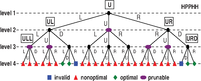
An example of a search tree is depicted in Figure 2. Leaf nodes represent configurations; some of them are invalid as they are not self-avoiding walks, such as configuration URDL; others are valid but do not achieve the highest possible number of contacts, such as configuration UUUU; finally, some are valid and optimal, such as configurations URDD and URDR. Without actually reaching all leaves, the algorithm is able to compute if a partial configuration, such as for example UU, cannot possibly lead to an optimal configuration and can prune computation early.

OPEN IN VIEWER

FIG. 2.

Search tree for sequence HPPHH. Level 0 is not represented, and the value of level 1, that is, the direction of the second bead is fixed at U, because the four branches of the root node are all equivalent up to rotations. Observe, furthermore, that all L-branches from the center, backbone of the tree are equivalent (specular) to their corresponding R-branches. Therefore, all corresponding calls are skipped. The left part of the tree is therefore not actually explored and is shown here only for the sake of clarity.

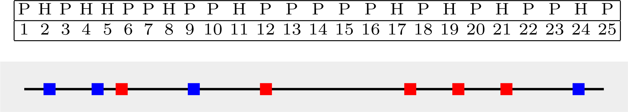
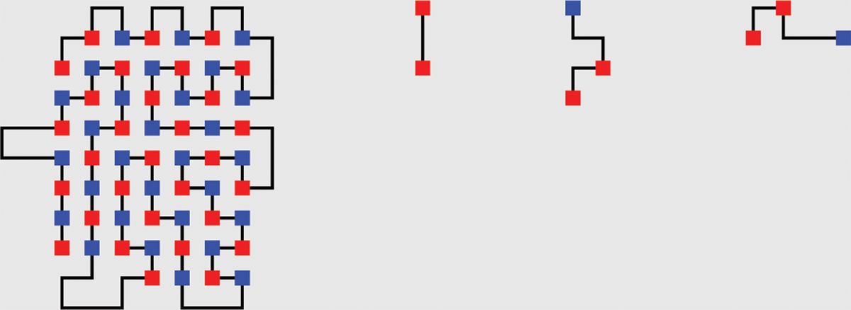
In Figure 3, we depict an example sequence of length 25, S _e  = PHPH²(PPH)²P⁵(HP)³PHP, which will guide us, as a running example, through the algorithm. In our pictures H beads are depicted as squares, and they are colored blue if they belong to \documentclass{aastex}\usepackage{amsbsy}\usepackage{amsfonts}\usepackage{amssymb}\usepackage{bm}\usepackage{mathrsfs}\usepackage{pifont}\usepackage{stmaryrd}\usepackage{textcomp}\usepackage{portland, xspace}\usepackage{amsmath, amsxtra}\pagestyle{empty}\DeclareMathSizes{10}{9}{7}{6}\begin{document} $${\cal H}_E$$ \end{document} and red if they belong to \documentclass{aastex}\usepackage{amsbsy}\usepackage{amsfonts}\usepackage{amssymb}\usepackage{bm}\usepackage{mathrsfs}\usepackage{pifont}\usepackage{stmaryrd}\usepackage{textcomp}\usepackage{portland, xspace}\usepackage{amsmath, amsxtra}\pagestyle{empty}\DeclareMathSizes{10}{9}{7}{6}\begin{document} $${\cal H}_O$$ \end{document} . P beads are not depicted, that is, they appear as a straight line that connects the sequence. Above the sequence, the index of each bead is shown, from 1 to 25. There are 4 Hs of type blue, and 5 Hs of type red. Hence, we have \documentclass{aastex}\usepackage{amsbsy}\usepackage{amsfonts}\usepackage{amssymb}\usepackage{bm}\usepackage{mathrsfs}\usepackage{pifont}\usepackage{stmaryrd}\usepackage{textcomp}\usepackage{portland, xspace}\usepackage{amsmath, amsxtra}\pagestyle{empty}\DeclareMathSizes{10}{9}{7}{6}\begin{document} $$\mid {\cal H}_E \mid = 4 , \mid {\cal H}_O \mid = 5$$ \end{document} , and C_parity = C_E = 8. Moreover, we have that \documentclass{aastex}\usepackage{amsbsy}\usepackage{amsfonts}\usepackage{amssymb}\usepackage{bm}\usepackage{mathrsfs}\usepackage{pifont}\usepackage{stmaryrd}\usepackage{textcomp}\usepackage{portland, xspace}\usepackage{amsmath, amsxtra}\pagestyle{empty}\DeclareMathSizes{10}{9}{7}{6}\begin{document} $$\mid {\cal H}_I \mid = 1$$ \end{document} and \documentclass{aastex}\usepackage{amsbsy}\usepackage{amsfonts}\usepackage{amssymb}\usepackage{bm}\usepackage{mathrsfs}\usepackage{pifont}\usepackage{stmaryrd}\usepackage{textcomp}\usepackage{portland, xspace}\usepackage{amsmath, amsxtra}\pagestyle{empty}\DeclareMathSizes{10}{9}{7}{6}\begin{document} $$\mid {\cal P}_S \mid = 3$$ \end{document} , so C_area = 10 and the stricter upper bound is given by C_parity. Consequently, in order to achieve eight contacts, all four H beads belonging to \documentclass{aastex}\usepackage{amsbsy}\usepackage{amsfonts}\usepackage{amssymb}\usepackage{bm}\usepackage{mathrsfs}\usepackage{pifont}\usepackage{stmaryrd}\usepackage{textcomp}\usepackage{portland, xspace}\usepackage{amsmath, amsxtra}\pagestyle{empty}\DeclareMathSizes{10}{9}{7}{6}\begin{document} $${\cal H}_E$$ \end{document} must achieve two contacts each. Observe that the energy of the optimal configuration(s) can be less than C_parity, that is, there might not be a configuration with such energy. In the case of the example sequence mentioned above, an optimal configuration with C_parity contacts (eight, in this case) does exist and is pictured in Figure 4.

OPEN IN VIEWER

FIG. 3.

(a) The sequence Se = PHPH²(PPH)²P⁵(HP)³PHP, of length 25, and the corresponding indexes of each bead; (b) graphical representation of Se. The link between sequence-adjacent beads is shown as a black segment. H beads are depicted as squares, and they are colored in blue if they belong to \documentclass{aastex}\usepackage{amsbsy}\usepackage{amsfonts}\usepackage{amssymb}\usepackage{bm}\usepackage{mathrsfs}\usepackage{pifont}\usepackage{stmaryrd}\usepackage{textcomp}\usepackage{portland, xspace}\usepackage{amsmath, amsxtra}\pagestyle{empty}\DeclareMathSizes{10}{9}{7}{6}\begin{document} $${\cal H}_E$$ \end{document} , and in red if they belong to \documentclass{aastex}\usepackage{amsbsy}\usepackage{amsfonts}\usepackage{amssymb}\usepackage{bm}\usepackage{mathrsfs}\usepackage{pifont}\usepackage{stmaryrd}\usepackage{textcomp}\usepackage{portland, xspace}\usepackage{amsmath, amsxtra}\pagestyle{empty}\DeclareMathSizes{10}{9}{7}{6}\begin{document} $${\cal H}_O$$ \end{document} . P beads are not depicted, that is, they appear as a straight line that connects the sequence. There are four blue Hs in this sequence (at indexes 2, 4, 8, 24), and five red Hs (at indexes 5, 11, 17, 19, 21).

OPEN IN VIEWER

FIG. 4.

The single, optimal configuration for the example sequence S _e . It has C_parity contacts (eight in this case: two for each of the blue beads).

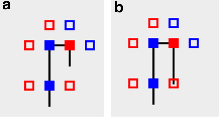
The main idea that we exploit in the proposed algorithm is based on the concept of exposed site. When a bead is placed on the lattice, it exposes sites where other beads must be located in order to create contacts. Hence, the placement of a bead imposes some constraints on a configuration, that is, it reduces the degrees of freedom and, consequently, makes it possible to predict if a partial configuration may or may not lead to an optimal configuration. In particular, we define the notion of weight of an exposed site and show how to use the information about the number and weight of exposed sites to state whether a configuration cannot yield a given, sought-after number of contacts. Figure 5a shows a partial configuration of an HP sequence, where three sites are exposed by O beads and two sites are exposed by E beads.

OPEN IN VIEWER

FIG. 5.

Partial configurations of the example sequence S _e : (a) Partial configuration UUURD. The H beads of types O and E are colored in red and blue, respectively. The link between sequence-adjacent beads is shown as a black segment. Empty squares are exposed sites. (b) Partial configuration UUURDD. The last placed P bead occupies a site exposed by the second bead and thus wastes a contact.

Formally, we define exposed site as an empty cell on the lattice that has at least one H bead as first-neighbor. We define the weight of an exposed site as the number of H beads that are first-neighbors of the site. The weight corresponds to the number of contacts that can be obtained by placing an H bead on the site. We say that an exposed site is of type O(E) if its first-neighbor(s) belong to the subset \documentclass{aastex}\usepackage{amsbsy}\usepackage{amsfonts}\usepackage{amssymb}\usepackage{bm}\usepackage{mathrsfs}\usepackage{pifont}\usepackage{stmaryrd}\usepackage{textcomp}\usepackage{portland, xspace}\usepackage{amsmath, amsxtra}\pagestyle{empty}\DeclareMathSizes{10}{9}{7}{6}\begin{document} $${\cal H}_O ({\cal H}_E)$$ \end{document} . Note that, analogously to the beads case, two exposed sites of the same type cannot be first-neighbors.

We define the state of a partial configuration as the tuple \documentclass{aastex}\usepackage{amsbsy}\usepackage{amsfonts}\usepackage{amssymb}\usepackage{bm}\usepackage{mathrsfs}\usepackage{pifont}\usepackage{stmaryrd}\usepackage{textcomp}\usepackage{portland, xspace}\usepackage{amsmath, amsxtra}\pagestyle{empty}\DeclareMathSizes{10}{9}{7}{6}\begin{document} \begin{align*}(C , (x_{\min} , y_{\min}) , (x_{\max} , y_{\max}) , W_O , W_E , S_O , S_E) ,\end{align*} \end{document}

where

We denote as h_E(k) the number of beads in \documentclass{aastex}\usepackage{amsbsy}\usepackage{amsfonts}\usepackage{amssymb}\usepackage{bm}\usepackage{mathrsfs}\usepackage{pifont}\usepackage{stmaryrd}\usepackage{textcomp}\usepackage{portland, xspace}\usepackage{amsmath, amsxtra}\pagestyle{empty}\DeclareMathSizes{10}{9}{7}{6}\begin{document} $${\cal H}_E$$ \end{document} that occur in the suffix of length n−k of the sequence, that is, \documentclass{aastex}\usepackage{amsbsy}\usepackage{amsfonts}\usepackage{amssymb}\usepackage{bm}\usepackage{mathrsfs}\usepackage{pifont}\usepackage{stmaryrd}\usepackage{textcomp}\usepackage{portland, xspace}\usepackage{amsmath, amsxtra}\pagestyle{empty}\DeclareMathSizes{10}{9}{7}{6}\begin{document} \begin{align*}h_E (k) = \mid \{i \mid i > k \wedge i \in {\cal H}_E \} \mid ,\tag{4}\end{align*} \end{document}

and h_O(k) is defined analogously. For the example sequence, h_E(15) = 1, h_O(15) = 3 (there is one remaining blue bead among the last 10 (25–15) beads, there are 3 remaining red beads among the last 10).

Our algorithm takes two input parameters in addition to the HP sequence. The first parameter is the number C_I ≤ min(C_parity,C_area) of expected contacts. Since the maximum number of contacts of the optimal configuration(s) is not known a priori, we parametrize it. The second parameter is the number Area_I, which is the maximum area of the H-core. The algorithm finds all the configurations of the sequence with a number of contacts equal at least to C_I and with H-core area equal at most to Area_I.

To find all the optimal configurations of a given sequence we proceed as follows. Given a sequence with contact bounds C_parity and C_area, we run the algorithm for each C_I value in the range 1, 2, … , min(C_parity,C_area) in decreasing order, in such a way that we can stop as soon as at least one configuration with the expected energy is found. Concerning the area parameter, given the parameter C_I we have to find a bound on the maximum area of any configuration of the sequence with C_I contacts. Values of Area_I below the maximum area are not safe as the algorithm could miss some or even all the configurations. Based on the results presented in Section 2.2, if C_I = C_area we use Equation 3 to compute the parameter Area_I from the semiperimeter \documentclass{aastex}\usepackage{amsbsy}\usepackage{amsfonts}\usepackage{amssymb}\usepackage{bm}\usepackage{mathrsfs}\usepackage{pifont}\usepackage{stmaryrd}\usepackage{textcomp}\usepackage{portland, xspace}\usepackage{amsmath, amsxtra}\pagestyle{empty}\DeclareMathSizes{10}{9}{7}{6}\begin{document} $$\lceil{\sqrt{2 A_{\min}} \rceil}$$ \end{document} , otherwise we set Area_I to ∞.

While traversing the search tree, the algorithm recursively computes the state associated with the partial configuration corresponding to the current node in the tree. It then evaluates various pruning criteria that allow one to establish whether the current partial configuration cannot yield a configuration with C_I contacts.

The pruning criteria that we discuss first are based on the parameter C_I. We say that a waste of w contacts occurs if an exposed site, with weight w, is occupied by a P bead. The maximum number of contacts that are exposed by the H beads of type O is C_O. Since we want to find all the configurations with at least C_I contacts, we can then waste at most \documentclass{aastex}\usepackage{amsbsy}\usepackage{amsfonts}\usepackage{amssymb}\usepackage{bm}\usepackage{mathrsfs}\usepackage{pifont}\usepackage{stmaryrd}\usepackage{textcomp}\usepackage{portland, xspace}\usepackage{amsmath, amsxtra}\pagestyle{empty}\DeclareMathSizes{10}{9}{7}{6}\begin{document} \begin{align*}W_O^{\max} = C_O - C_I\end{align*} \end{document}

contacts exposed by H beads of type O. The same consideration holds for the H beads of type E. Note that, since C_I ≤ C_parity = min(C_E, C_O), both \documentclass{aastex}\usepackage{amsbsy}\usepackage{amsfonts}\usepackage{amssymb}\usepackage{bm}\usepackage{mathrsfs}\usepackage{pifont}\usepackage{stmaryrd}\usepackage{textcomp}\usepackage{portland, xspace}\usepackage{amsmath, amsxtra}\pagestyle{empty}\DeclareMathSizes{10}{9}{7}{6}\begin{document} $$W_O^{\max}$$ \end{document} and \documentclass{aastex}\usepackage{amsbsy}\usepackage{amsfonts}\usepackage{amssymb}\usepackage{bm}\usepackage{mathrsfs}\usepackage{pifont}\usepackage{stmaryrd}\usepackage{textcomp}\usepackage{portland, xspace}\usepackage{amsmath, amsxtra}\pagestyle{empty}\DeclareMathSizes{10}{9}{7}{6}\begin{document} $$W_E^{\max}$$ \end{document} are non-negative and thus well defined. The pruning criterion is then:

 Criterion 1. If WE >  \documentclass{aastex}\usepackage{amsbsy}\usepackage{amsfonts}\usepackage{amssymb}\usepackage{bm}\usepackage{mathrsfs}\usepackage{pifont}\usepackage{stmaryrd}\usepackage{textcomp}\usepackage{portland, xspace}\usepackage{amsmath, amsxtra}\pagestyle{empty}\DeclareMathSizes{10}{9}{7}{6}\begin{document} $$W_E^{\max}$$ \end{document} or WO >  \documentclass{aastex}\usepackage{amsbsy}\usepackage{amsfonts}\usepackage{amssymb}\usepackage{bm}\usepackage{mathrsfs}\usepackage{pifont}\usepackage{stmaryrd}\usepackage{textcomp}\usepackage{portland, xspace}\usepackage{amsmath, amsxtra}\pagestyle{empty}\DeclareMathSizes{10}{9}{7}{6}\begin{document} $$W_O^{max}$$ \end{document} , the current configuration is prunable.

Figure 5b shows a partial configuration of the example sequence S _e in which one site of type E with unitary weight is wasted, that is, W_E = 1. If C_I = C_parity, it follows that \documentclass{aastex}\usepackage{amsbsy}\usepackage{amsfonts}\usepackage{amssymb}\usepackage{bm}\usepackage{mathrsfs}\usepackage{pifont}\usepackage{stmaryrd}\usepackage{textcomp}\usepackage{portland, xspace}\usepackage{amsmath, amsxtra}\pagestyle{empty}\DeclareMathSizes{10}{9}{7}{6}\begin{document} $$W_E^{\max} = 0$$ \end{document} , and thus the partial configuration is prunable, as it cannot possibly lead to an optimal configuration of C_parity contacts.

The next pruning criterion relates to exposed sites. Observe that the minimum number of exposed sites of type O that must be occupied, in order to not waste more than \documentclass{aastex}\usepackage{amsbsy}\usepackage{amsfonts}\usepackage{amssymb}\usepackage{bm}\usepackage{mathrsfs}\usepackage{pifont}\usepackage{stmaryrd}\usepackage{textcomp}\usepackage{portland, xspace}\usepackage{amsmath, amsxtra}\pagestyle{empty}\DeclareMathSizes{10}{9}{7}{6}\begin{document} $$W_O^{\max}$$ \end{document} −W_O contacts, is equal to \documentclass{aastex}\usepackage{amsbsy}\usepackage{amsfonts}\usepackage{amssymb}\usepackage{bm}\usepackage{mathrsfs}\usepackage{pifont}\usepackage{stmaryrd}\usepackage{textcomp}\usepackage{portland, xspace}\usepackage{amsmath, amsxtra}\pagestyle{empty}\DeclareMathSizes{10}{9}{7}{6}\begin{document} \begin{align*}S_O - (W_O^{\max} - W_O)\end{align*} \end{document}

because, in the most conservative case, each site has unitary weight, and thus we can waste at most a number of sites equal to the number of wastable contacts; the same reasoning holds for the sites of type E. It follows that the number of H beads in the remaining suffix of the sequence (defined by the map h_O(·) in Eq. 4) must be equal at least to the number of exposed sites that have to be occupied. Given a partial configuration of length k, the pruning criterion is then:

 Criterion 2. If h_O(k) < S_E−( \documentclass{aastex}\usepackage{amsbsy}\usepackage{amsfonts}\usepackage{amssymb}\usepackage{bm}\usepackage{mathrsfs}\usepackage{pifont}\usepackage{stmaryrd}\usepackage{textcomp}\usepackage{portland, xspace}\usepackage{amsmath, amsxtra}\pagestyle{empty}\DeclareMathSizes{10}{9}{7}{6}\begin{document} $$W_E^{\max} - W_E$$ \end{document} ) or h_E(k) < S_O−( \documentclass{aastex}\usepackage{amsbsy}\usepackage{amsfonts}\usepackage{amssymb}\usepackage{bm}\usepackage{mathrsfs}\usepackage{pifont}\usepackage{stmaryrd}\usepackage{textcomp}\usepackage{portland, xspace}\usepackage{amsmath, amsxtra}\pagestyle{empty}\DeclareMathSizes{10}{9}{7}{6}\begin{document} $$W_O^{\max} - W_O$$ \end{document} ), the current configuration is prunable.

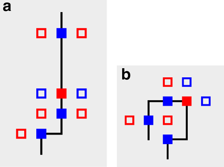
Figure 6a shows a partial configuration of the example sequence S _e in which there are not enough remaining beads of type O that may occupy the exposed sites of type E. Specifically, we have h_O(8) = 4, S_E = 5, and W_E = 0. Hence, if C_I = C_parity, the configuration is prunable.

OPEN IN VIEWER

FIG. 6.

Partial configurations of the example sequence S _e : (a) Partial configuration URUUUUUU. There are four beads of type O left; hence, it is not possible to occupy all the sites exposed by the beads of type E (there are five of them). This situation will result necessarily in wasting at least a contact, and therefore C_parity cannot be achieved. Hence, this configuration is prunable. (b) Partial configuration UURRDDLD showing an unreachable exposed site with weight 3.

We now focus on the number of contacts of a given configuration. In particular, we try to estimate the maximum number of remaining contacts achievable by a given partial configuration. If this number is smaller than C_I−C, (C is the current number of contacts of the partial configuration), we may conclude that the current configuration cannot yield C_I contacts. A pruning criterion follows:

 Criterion 3. Let C_left be the maximum number of remaining contacts that can be achieved by the current configuration. If C_left < (C_I−C), the current configuration is prunable.

We show next how to estimate C_left. The first observation concerns the number of contacts that an H bead generates when placed on the lattice. By Lemma 1, any internal bead can make at most two contacts while the last bead can make at most three contacts. Moreover, note that the last bead can make three contacts only if it is an H bead. Obviously, the placement of the first bead does not give rise to any contact. This fact leads to a simple loose estimate of the maximum number of contacts achievable by a partial configuration of length k: \documentclass{aastex}\usepackage{amsbsy}\usepackage{amsfonts}\usepackage{amssymb}\usepackage{bm}\usepackage{mathrsfs}\usepackage{pifont}\usepackage{stmaryrd}\usepackage{textcomp}\usepackage{portland, xspace}\usepackage{amsmath, amsxtra}\pagestyle{empty}\DeclareMathSizes{10}{9}{7}{6}\begin{document} \begin{align*}2 (h_E (k) + h_O (k)) + e_n\end{align*} \end{document}

where e_n is 1 if â_n = H and 0 otherwise. However, it is possible to obtain a closer (i.e., correct but less conservative) estimate by exploiting the information on the number and weight of the existing exposed sites. As explained above, an H bead, when placed on the lattice, exposes either two sites if it is internal or three if it is the first or the last bead; to generate contacts, the exposed sites must be occupied by a bead of the opposite type. There are three main conditions under which an exposed site cannot be occupied by such a bead with a resulting waste equal to the corresponding weight:

Figure 6a and 6b shows examples of Conditions 2 and 3. Let 1 ≤ k < n be the length of a given partial configuration. We focus on the beads of type O, but the reasoning is analogous for the other case. A crucial observation is that the beads cannot make more than \documentclass{aastex}\usepackage{amsbsy}\usepackage{amsfonts}\usepackage{amssymb}\usepackage{bm}\usepackage{mathrsfs}\usepackage{pifont}\usepackage{stmaryrd}\usepackage{textcomp}\usepackage{portland, xspace}\usepackage{amsmath, amsxtra}\pagestyle{empty}\DeclareMathSizes{10}{9}{7}{6}\begin{document} $$2 \mid {\cal H}_O \mid + e_1 + e_O$$ \end{document} contacts (see Eq. 1), which implies that we can estimate the number of potential residual contacts by considering the H beads and the exposed sites of type O only. We can write the maximum number of remaining contacts as C₁+C₂, where C₁ and C₂ are the contacts achievable by the remaining and placed beads, respectively. As for the beads that have not been placed yet, we assume that the most favorable case applies, that is, C₁ = 2h_O(k)+e_O. Let s_O(i) be the number of exposed sites of type O with weight i, for \documentclass{aastex}\usepackage{amsbsy}\usepackage{amsfonts}\usepackage{amssymb}\usepackage{bm}\usepackage{mathrsfs}\usepackage{pifont}\usepackage{stmaryrd}\usepackage{textcomp}\usepackage{portland, xspace}\usepackage{amsmath, amsxtra}\pagestyle{empty}\DeclareMathSizes{10}{9}{7}{6}\begin{document} $$i = 1 , \ldots , 4$$ \end{document} ; s_E is defined analogously. Concerning the placed beads, the respective number of potential contacts is 2( \documentclass{aastex}\usepackage{amsbsy}\usepackage{amsfonts}\usepackage{amssymb}\usepackage{bm}\usepackage{mathrsfs}\usepackage{pifont}\usepackage{stmaryrd}\usepackage{textcomp}\usepackage{portland, xspace}\usepackage{amsmath, amsxtra}\pagestyle{empty}\DeclareMathSizes{10}{9}{7}{6}\begin{document} $$\mid {\cal H}_O \mid - h_O (k)$$ \end{document} )+e₁. However, the following inequality holds: \documentclass{aastex}\usepackage{amsbsy}\usepackage{amsfonts}\usepackage{amssymb}\usepackage{bm}\usepackage{mathrsfs}\usepackage{pifont}\usepackage{stmaryrd}\usepackage{textcomp}\usepackage{portland, xspace}\usepackage{amsmath, amsxtra}\pagestyle{empty}\DeclareMathSizes{10}{9}{7}{6}\begin{document} \begin{align*}C_2 \le \sum_{i = 1}^{4}i \cdot s_O (i) \le 2 (\mid {\cal H}_O \mid - h_O (k)) + e_1 - C ,\end{align*} \end{document}

that is, the weighted sum of the exposed sites is the maximum number of contacts still achievable by the placed beads, and it cannot exceed the number of potential contacts minus the existing contacts. Hence, we can use \documentclass{aastex}\usepackage{amsbsy}\usepackage{amsfonts}\usepackage{amssymb}\usepackage{bm}\usepackage{mathrsfs}\usepackage{pifont}\usepackage{stmaryrd}\usepackage{textcomp}\usepackage{portland, xspace}\usepackage{amsmath, amsxtra}\pagestyle{empty}\DeclareMathSizes{10}{9}{7}{6}\begin{document} $$C_2 = \sum_{i = 1}^{4}i \cdot s_O (i)$$ \end{document} . Observe that the number of contacts wasted because of Condition 1, that is, W_O, is equal to the third term minus the second term. When such two quantities are equal, no site is wasted; instead, if the difference is positive, one or more sites are wasted, because when a site is occupied by a P bead, the number of exposed sites decreases while C does not increase. To take into account Conditions 2 and 3, we need a tighter bound for the term \documentclass{aastex}\usepackage{amsbsy}\usepackage{amsfonts}\usepackage{amssymb}\usepackage{bm}\usepackage{mathrsfs}\usepackage{pifont}\usepackage{stmaryrd}\usepackage{textcomp}\usepackage{portland, xspace}\usepackage{amsmath, amsxtra}\pagestyle{empty}\DeclareMathSizes{10}{9}{7}{6}\begin{document} $$\sum \nolimits _{i = 1}^{4}i \cdot s_O (i)$$ \end{document} . Observe that the sites with weight 4 cannot be reached and only one site with weight 3 can be occupied (by the last bead, provided that it is an H bead of type E). Moreover, note that we cannot occupy more than h_E(k) sites, as we would not have enough beads available. In order to account for the most conservative scenario, we assume that the sites with highest weights are occupied. The number of sites that can be effectively occupied is then \documentclass{aastex}\usepackage{amsbsy}\usepackage{amsfonts}\usepackage{amssymb}\usepackage{bm}\usepackage{mathrsfs}\usepackage{pifont}\usepackage{stmaryrd}\usepackage{textcomp}\usepackage{portland, xspace}\usepackage{amsmath, amsxtra}\pagestyle{empty}\DeclareMathSizes{10}{9}{7}{6}\begin{document} $$M_O = M_O^3 + M_O^2 + M_O^1 \le S_O$$ \end{document} , where \documentclass{aastex}\usepackage{amsbsy}\usepackage{amsfonts}\usepackage{amssymb}\usepackage{bm}\usepackage{mathrsfs}\usepackage{pifont}\usepackage{stmaryrd}\usepackage{textcomp}\usepackage{portland, xspace}\usepackage{amsmath, amsxtra}\pagestyle{empty}\DeclareMathSizes{10}{9}{7}{6}\begin{document} \begin{align*} & M_O^3 = \min (s_O (3) , e_E) \\ & M_O^2 = \min (s_O (2) , h_E (k) - M_O^3) \\ & M_O^1 = \min (s_O (1) , h_E (k) - M_O^3 - M_O^2) \end{align*} \end{document}

Hence, if M_O < S_O, we waste \documentclass{aastex}\usepackage{amsbsy}\usepackage{amsfonts}\usepackage{amssymb}\usepackage{bm}\usepackage{mathrsfs}\usepackage{pifont}\usepackage{stmaryrd}\usepackage{textcomp}\usepackage{portland, xspace}\usepackage{amsmath, amsxtra}\pagestyle{empty}\DeclareMathSizes{10}{9}{7}{6}\begin{document} $$\sum_{i = 0}^4 i (s_O (i) - M_O^i)$$ \end{document} contacts because of Conditions 2 and/or 3. Summing up, the resulting formula is: \documentclass{aastex}\usepackage{amsbsy}\usepackage{amsfonts}\usepackage{amssymb}\usepackage{bm}\usepackage{mathrsfs}\usepackage{pifont}\usepackage{stmaryrd}\usepackage{textcomp}\usepackage{portland, xspace}\usepackage{amsmath, amsxtra}\pagestyle{empty}\DeclareMathSizes{10}{9}{7}{6}\begin{document} \begin{align*}2h_O (k) + e_O + 3M_O^3 + 2M_O^2 + M_O^1\end{align*} \end{document}

The next pruning criterion concerns the H-core, that is, the smallest rectangle containing all the H beads placed in the current configuration:

 Criterion 4. If the area of the H-core encoded by the coordinates (x_min, y_min),(x_max, y_max) is bigger than Area_I, the current configuration is prunable.

We recall that Area_I is the parameter of the algorithm that specifies the maximum area of the H-core. Observe that the parameter Area_I is constrained by the inequality Area_I ≥ A_min. Moreover, note that the maximum number of nonsinglet P beads in the H-core is bounded by Area_I−A_min; otherwise, the H-core could not contain all the H beads. This observation leads to another pruning criterion:

 Criterion 5. If the number of nonsinglet P beads in the current H-core is greater than Area_I−A_min, the current configuration is prunable.

When C_I = C_area, we can also devise another pruning criterion, based on Theorem 1. By Theorem 1 and the definition of φ, it follows that in any connected H-core with dimensions (L₁, L₂), m H beads and φ(L₁ + L₂) contacts the waste must be exactly 2(L₁L₂−m), that is, \documentclass{aastex}\usepackage{amsbsy}\usepackage{amsfonts}\usepackage{amssymb}\usepackage{bm}\usepackage{mathrsfs}\usepackage{pifont}\usepackage{stmaryrd}\usepackage{textcomp}\usepackage{portland, xspace}\usepackage{amsmath, amsxtra}\pagestyle{empty}\DeclareMathSizes{10}{9}{7}{6}\begin{document} \begin{align*}\sum_{i \in R_P} (n_H (i , *) - 1) + \sum_{j \in C_P} (n_H (* ,\ j) - 1) = 0 ,\end{align*} \end{document}

where we recall that n_H is the number of H beads in a row (column) after collapsing all the sequences of adjacent H beads into a single H bead. Moreover, it is a simple observation that in a configuration with semiperimeter \documentclass{aastex}\usepackage{amsbsy}\usepackage{amsfonts}\usepackage{amssymb}\usepackage{bm}\usepackage{mathrsfs}\usepackage{pifont}\usepackage{stmaryrd}\usepackage{textcomp}\usepackage{portland, xspace}\usepackage{amsmath, amsxtra}\pagestyle{empty}\DeclareMathSizes{10}{9}{7}{6}\begin{document} $$\lceil{2 \sqrt{A_{\min}} \rceil}$$ \end{document} , which is the smallest semiperimeter possible to contain the whole sequence, we have n_H ≥ 1 for any row and column, that is, each row and column contains at least one H bead. This observation leads to our final pruning criterion:

 Criterion 6. If C_I = C_area and there is one row or column with n_H > 1, the current configuration is prunable.

The criterion in practice says that in a configuration with C_area contacts, there cannot be in any row or in any column a segment of Ps delimited by Hs at each end. Figure 7 exemplifies this concept: a benchmark sequence is pictured, S1 - 9, with one of its optimal configurations. The picture then shows three partial configurations that are pruned because of Criterion 6. In fact, in all three cases we have a segment of Ps delimited by Hs: in the first and second case this happens along a column, while in the third case it happens along a row.

OPEN IN VIEWER

FIG. 7.

Example of how early in the search Criterion 6 is able to prune. The picture shows an optimal configuration for sequence S1-9 (reversed), and three partial configurations that are pruned because of Criterion 6. The first partial configuration is pruned as early as the third bead, and the second and third configuration as early as the fifth bead.

One important thing to notice is how early in the search this criterion is able to prune: already in the third or fifth bead, in a sequence of length 64. Notice that, instead, the criteria based on exposed sites would not be effective, in this case, this early in the search. Criterion 6, in combination with Criterion 5, is indeed the main reason minwalk performs so effectively in those benchmark sequences where the optimal number of contacts is equal to the upper bound C_area.