Gene regulatory network inference (that is, determination of the regulatory interactions between a set of genes) provides mechanistic insights of central importance to research in systems biology. Most contemporary network inference methods rely on a sparsity/regularization coefficient, which we call ζ (zeta), to determine the degree of sparsity of the network estimates, that is, the total number of links between the nodes. However, they offer little or no advice on how to select this sparsity coefficient, in particular, for biological data with few samples. We show that an empty network is more accurate than estimates obtained for a poor choice of ζ. In order to avoid such poor choices, we propose a method for optimization of ζ, which maximizes the accuracy of the inferred network for any sparsity-dependent inference method and data set. Our procedure is based on leave-one-out cross-optimization and selection of the ζ value that minimizes the prediction error. We also illustrate the adverse effects of noise, few samples, and uninformative experiments on network inference as well as our method for optimization of ζ. We demonstrate that our ζ optimization method for two widely used inference algorithms—Glmnet and NIR—gives accurate and informative estimates of the network structure, given that the data is informative enough.
1. Introduction
Gene regulatory networks (GRNs) model the mechanistic interactions among genes, giving insight into how signals among genes are propagated through the genetic network and how genes respond to exogenous and endogenous stimuli. Much work has been done on developing and evaluating algorithms for inference of regulatory networks from perturbations and responses in expression data (Bansal et al., 2007; He et al., 2009; Hache et al., 2009a; Marbach et al., 2010). The primary goal is to find the structure of the network, that is, the interactions that exist within the set of nodes. Accurate prediction of the observed responses is in general not sufficient for accurate estimation of the network structure. Most contemporary inference methods rely on a sparsity/regularization coefficient, which we call ζ (zeta), to control the degree of sparsity of the network estimates (that is, the number of links between the nodes). They however offer little or no advice on how to select this sparsity coefficient, even though it is typically crucial for accurate estimation of the structure. In particular, the low number of samples encountered in biological data sets is problematic and makes it unclear if classical model selection and cross-validation strategies work. We therefore investigated if the optimal ζ value can be found based on the prediction error for data with a low number of samples, and as a result, propose a method for optimization of ζ, which maximizes the accuracy of the inferred network for a given inference method and data set. We apply our method to three in silico data sets with varying information content and demonstrate that our method works well when the data is informative enough.
By selecting the sparsity coefficient, one in general determines the trade-off between accuracy of data prediction and model complexity. Classical model selection criteria, such as Akaike information criterion (AIC), Bayesian information criterion (BIC), and cross-validation, have long been studied and shown to perform a good trade-off under certain conditions, in particular, when the number of samples is large and the model is used for data prediction (Stoica and Selen, 2004). These classical methods have been used in a few studies for selection of the regularization coefficient during the past decade, including applications to biological data (Fan and Li, 2001; Thorsson and Michael, 2005; Wang et al., 2007; Lian, 2009; Friedman et al., 2010; Menéndez et al., 2010; Demir-Kavuk et al., 2011). The BIC (Wang et al., 2007; Lian, 2009; Menéndez et al., 2010) is shown to be favorable over the other criteria tested in their study, while Thorsson and Michael (2005) found selection based on minimization of the prediction error in cross-validation and bootstraping to be favorable over AIC and BIC. Cross-validation (Bonneau et al., 2006; Friedman et al., 2010) is used for selection of the regularization coefficient in LASSO, but they instead chose the value corresponding to the sparsest model within one standard error from the minimum to decrease the number of false positives. Selection of the sparsity coefficient in network inference is only studied in Menéndez et al. (2010). In vivo data (Bonneau et al., 2006) is used to infer the GRN of Halobacterium, and the researchers selected ζ, but the “true” network is unknown and the performance can therefore not be properly evaluated. In silico data from the DREAM4 challenge (Menéndez et al., 2010) is used for method evaluation, but the signed topology that we are interested in is not considered. Networks with 100 genes were used to generate their data, simulating 100 multifactorial steady-state perturbation experiments. We consider a similar network inference case but use a small network and systematically vary data properties to gain insight on how to select ζ for three different inference algorithms. We focus on the relation between the prediction error and topological accuracy in network inference from data with few samples and do not therefore consider rules that make a specific trade-off between predictive ability and model complexity, such as AIC and BIC.
The use of simulated data from gold standard networks for evaluation of network inference algorithms is standard nowadays. Several in silico network and data-generating software programs have therefore been created (Mendes et al., 2003; Hache et al., 2009b; Schaffter et al., 2011). These tools use varying modeling approaches and biological mechanisms to simulate biological networks and network motifs. Data sets based on simpler, directly generated, linear ordinary differential equation (ODE) models have also been used in benchmarking (Bansal et al., 2007). For simplicity and control of network and data properties, we use a linear ODE model for data generation.
2. Problem Description
Throughout this article, we consider a system that can be approximated as first order linear ODEs:
\documentclass{aastex}\usepackage{amsbsy}\usepackage{amsfonts}\usepackage{amssymb}\usepackage{bm}\usepackage{mathrsfs}\usepackage{pifont}\usepackage{stmaryrd}\usepackage{textcomp}\usepackage{portland, xspace}\usepackage{amsmath, amsxtra}\pagestyle{empty}\DeclareMathSizes{10}{9}{7}{6}\begin{document}\begin{align*}\begin{split} & \dot{x}_i ( t ) = \sum\nolimits_{j = 1}^N
a_{ij}x_j ( t ) + p_i ( t ) - f_i ( t ) \\ & y_i ( t ) = x_i ( t )
+ e_i ( t ) \end{split} \tag{1}\end{align*}\end{document}
where the state vector \documentclass{aastex}\usepackage{amsbsy}\usepackage{amsfonts}\usepackage{amssymb}\usepackage{bm}\usepackage{mathrsfs}\usepackage{pifont}\usepackage{stmaryrd}\usepackage{textcomp}\usepackage{portland, xspace}\usepackage{amsmath, amsxtra}\pagestyle{empty}\DeclareMathSizes{10}{9}{7}{6}\begin{document}$$\textbf{\textit{x}} ( t ) = [ x_1 ( t ) , x_2 ( t ) , \ldots , x_N ( t ) ] ^T$$\end{document} represents actual mRNA expression changes relative to the initial state of the system. The vector \documentclass{aastex}\usepackage{amsbsy}\usepackage{amsfonts}\usepackage{amssymb}\usepackage{bm}\usepackage{mathrsfs}\usepackage{pifont}\usepackage{stmaryrd}\usepackage{textcomp}\usepackage{portland, xspace}\usepackage{amsmath, amsxtra}\pagestyle{empty}\DeclareMathSizes{10}{9}{7}{6}\begin{document}$$\textbf{\textit{p}} ( t ) = [ p_1 ( t ) , p_2 ( t ) , \ldots , p_N ( t ) ] ^T$$\end{document} is the desired or measured perturbation that differs from the applied one by the noise f(t), and \documentclass{aastex}\usepackage{amsbsy}\usepackage{amsfonts}\usepackage{amssymb}\usepackage{bm}\usepackage{mathrsfs}\usepackage{pifont}\usepackage{stmaryrd}\usepackage{textcomp}\usepackage{portland, xspace}\usepackage{amsmath, amsxtra}\pagestyle{empty}\DeclareMathSizes{10}{9}{7}{6}\begin{document}$$\textbf{\textit{y}} ( t ) = [ y_1 ( t ) , y_2 ( t ) , \ldots , y_N ( t ) ] ^T$$\end{document} is the measured response that differs from the expression changes by the noise e(t). The parameters aij of the interaction matrix describe the influence of gene j on gene i. A positive value represents an activation, while a negative value represents an inhibition. The relative strength of the interaction is given by the value of the parameter. We make the common assumption that only steady state data is recorded and write the system in matrix notation as
\documentclass{aastex}\usepackage{amsbsy}\usepackage{amsfonts}\usepackage{amssymb}\usepackage{bm}\usepackage{mathrsfs}\usepackage{pifont}\usepackage{stmaryrd}\usepackage{textcomp}\usepackage{portland, xspace}\usepackage{amsmath, amsxtra}\pagestyle{empty}\DeclareMathSizes{10}{9}{7}{6}\begin{document}\begin{align*}
\textbf{\textit{Y}} = -
\textbf{\textit{A}}^\textbf{\textit{-1}}\textbf{\textit{P}} +
\textbf{\textit{A}}^\textbf{\textit{-1}}\textbf{\textit{F}} +
\textbf{\textit{E}}. \tag{2}
\end{align*}\end{document}
Here, Y is our steady state expression matrix after applying the perturbations P, and A is the interaction matrix. This type of linear data model has previously been used when inferring gene regulatory networks (Gardner et al., 2003; Julius et al., 2009; Lorenz et al., 2009; Nordling and Jacobsen, 2009; Jörnsten et al., 2011). In this case, the goal of network inference corresponds to inference of the structure of the interaction matrix A.
To obtain sparse network models, a variety of methods that either directly or indirectly place a weight or constraint on the model complexity in terms of the number of nonzero parameters aij have been developed in several fields (Stoica and Selen, 2004; Fan and Li, 2006; Candes and Wakin, 2008; Hecker et al., 2009; Fan and Lv, 2010;). The idea is to exclude less influential interactions while keeping the most influential ones, in terms of ability to predict experimental observations by penalizing small nonzero parameters. To accomplish this, a method-specific sparsity/regularization coefficient, which we here denote \documentclass{aastex}\usepackage{amsbsy}\usepackage{amsfonts}\usepackage{amssymb}\usepackage{bm}\usepackage{mathrsfs}\usepackage{pifont}\usepackage{stmaryrd}\usepackage{textcomp}\usepackage{portland, xspace}\usepackage{amsmath, amsxtra}\pagestyle{empty}\DeclareMathSizes{10}{9}{7}{6}\begin{document}$$\tilde{\zeta}$$\end{document} and later standardize such that \documentclass{aastex}\usepackage{amsbsy}\usepackage{amsfonts}\usepackage{amssymb}\usepackage{bm}\usepackage{mathrsfs}\usepackage{pifont}\usepackage{stmaryrd}\usepackage{textcomp}\usepackage{portland, xspace}\usepackage{amsmath, amsxtra}\pagestyle{empty}\DeclareMathSizes{10}{9}{7}{6}\begin{document}$$\zeta \in [ 0 , 1 ]$$\end{document}, is used in most methods to set the weight or constraint on the number of links, like in the LASSO method (Tibshirani, 1996)
\documentclass{aastex}\usepackage{amsbsy}\usepackage{amsfonts}\usepackage{amssymb}\usepackage{bm}\usepackage{mathrsfs}\usepackage{pifont}\usepackage{stmaryrd}\usepackage{textcomp}\usepackage{portland, xspace}\usepackage{amsmath, amsxtra}\pagestyle{empty}\DeclareMathSizes{10}{9}{7}{6}\begin{document}\begin{align*}
\hat{\textbf{\textit{A}}}_{\rm reg} (\tilde{ \zeta}) = \arg
\min_\textbf{\textit{A}} \| \textbf{\textit{AY}} +
\textbf{\textit{P}} \| _{l_2} + \tilde{\zeta} \|
\textbf{\textit{A}} \| _{l_1} , \tag{3}
\end{align*}\end{document}
which is one of the most well-known ones. Several conditions for near ideal model selection have been established for certain methods, in particular given a suitable choice of ζ (Wang et al., 2007; Candès and Plan, 2009; Fan and Lv, 2010), but how to choose ζ based on data sets with a low number of samples is still an open problem. Therefore, we studied how the selection of ζ affects the network estimate for data sets of the type common in systems biology. The idea is to investigate, through numerical simulations and analysis, if an efficient method for selection of ζ that can be wrapped around implementations of existing inference methods could be developed. In order to be efficient, the method must select a ζ value such that no network estimate that is structurally more similar to the “true” network exists for any other choice of ζ for that particular inference method. As a result, we propose such a method.
3. Methods
3.1. Pretreatment of data
A model is only useful for prediction of experiments similar to the ones from which it was estimated, so the validation set should only contain experiments that are linearly dependent on the experiments in the training set.
We therefore measure the degree of linear dependence between an experiment yk and the ones in the training set Yt≠k as
\documentclass{aastex}\usepackage{amsbsy}\usepackage{amsfonts}\usepackage{amssymb}\usepackage{bm}\usepackage{mathrsfs}\usepackage{pifont}\usepackage{stmaryrd}\usepackage{textcomp}\usepackage{portland, xspace}\usepackage{amsmath, amsxtra}\pagestyle{empty}\DeclareMathSizes{10}{9}{7}{6}\begin{document}\begin{align*}
\eta_{y_k} \triangleq \| \textbf{\textit{Y}}_{t \neq k}^T
\textbf{\textit{y}}_{k} \|_1 \tag{4}
\end{align*}\end{document}
and similarly for the perturbations. All directions of the system are sufficiently excited in the examples that we provide later on, and we therefore use the smallest singular value σN as our limit on η. The index set of the validation experiments is hence
\documentclass{aastex}\usepackage{amsbsy}\usepackage{amsfonts}\usepackage{amssymb}\usepackage{bm}\usepackage{mathrsfs}\usepackage{pifont}\usepackage{stmaryrd}\usepackage{textcomp}\usepackage{portland, xspace}\usepackage{amsmath, amsxtra}\pagestyle{empty}\DeclareMathSizes{10}{9}{7}{6}\begin{document}\begin{align*}{ \cal V} \ \triangleq \{ k \mid
\eta_{\textbf{\textit{y}}_k} \geq \sigma_N ( \textbf{\textit{Y}})
\ {\rm and} \eta_{\textbf{\textit{p}}_k} \geq \sigma_N
(\textbf{\textit{P}}) \} . \tag{5}\end{align*}\end{document}
The sparsity of the estimated network for a specific ζ value depends on both the data and the algorithm used. To simplify the comparison between different data sets and algorithms, we therefore standardize ζ, such that an empty network is obtained for ζ = 1 and a full network for ζ = 0. For Glmnet and LSCO, the standardized ζ is equal to the actual \documentclass{aastex}\usepackage{amsbsy}\usepackage{amsfonts}\usepackage{amssymb}\usepackage{bm}\usepackage{mathrsfs}\usepackage{pifont}\usepackage{stmaryrd}\usepackage{textcomp}\usepackage{portland, xspace}\usepackage{amsmath, amsxtra}\pagestyle{empty}\DeclareMathSizes{10}{9}{7}{6}\begin{document}$$\tilde{ \zeta}$$\end{document} divided by the smallest \documentclass{aastex}\usepackage{amsbsy}\usepackage{amsfonts}\usepackage{amssymb}\usepackage{bm}\usepackage{mathrsfs}\usepackage{pifont}\usepackage{stmaryrd}\usepackage{textcomp}\usepackage{portland, xspace}\usepackage{amsmath, amsxtra}\pagestyle{empty}\DeclareMathSizes{10}{9}{7}{6}\begin{document}$$\tilde{ \zeta}$$\end{document}, such that the network estimate \documentclass{aastex}\usepackage{amsbsy}\usepackage{amsfonts}\usepackage{amssymb}\usepackage{bm}\usepackage{mathrsfs}\usepackage{pifont}\usepackage{stmaryrd}\usepackage{textcomp}\usepackage{portland, xspace}\usepackage{amsmath, amsxtra}\pagestyle{empty}\DeclareMathSizes{10}{9}{7}{6}\begin{document}$$ \hat {\textbf{\textit{A}}}_{{ \rm reg}} = 0 $$\end{document} for all different training data sets \documentclass{aastex}\usepackage{amsbsy}\usepackage{amsfonts}\usepackage{amssymb}\usepackage{bm}\usepackage{mathrsfs}\usepackage{pifont}\usepackage{stmaryrd}\usepackage{textcomp}\usepackage{portland, xspace}\usepackage{amsmath, amsxtra}\pagestyle{empty}\DeclareMathSizes{10}{9}{7}{6}\begin{document}$$\{ \textbf{\textit{Y}}_{t \neq k} , \textbf{\textit{P}}_{t \neq k} \} $$\end{document}. For NIR (Di Bernardo et al., 2004), the standardized ζ is (\documentclass{aastex}\usepackage{amsbsy}\usepackage{amsfonts}\usepackage{amssymb}\usepackage{bm}\usepackage{mathrsfs}\usepackage{pifont}\usepackage{stmaryrd}\usepackage{textcomp}\usepackage{portland, xspace}\usepackage{amsmath, amsxtra}\pagestyle{empty}\DeclareMathSizes{10}{9}{7}{6}\begin{document}$$( N - \tilde{ \zeta} ) / N$$\end{document}).
3.2. Leave-one-out cross-optimization
When few experiments exist, use of the whole data set to predict the network might be an attractive option, but it would lead to overfitting of the parameters to noise. As the number of observations tend to be small, we employ a leave-one-out cross-optimization (LOOCO) scheme, where each experiment k that fulfills Equation (5) in turn is left out, and the remaining t ≠ k experiments are used to estimate the model \documentclass{aastex}\usepackage{amsbsy}\usepackage{amsfonts}\usepackage{amssymb}\usepackage{bm}\usepackage{mathrsfs}\usepackage{pifont}\usepackage{stmaryrd}\usepackage{textcomp}\usepackage{portland, xspace}\usepackage{amsmath, amsxtra}\pagestyle{empty}\DeclareMathSizes{10}{9}{7}{6}\begin{document}$$\hat {\textbf{\textit{A}}}$$\end{document}. After re-estimation of the parameters, this model is then used to predict the response in kth experiment.
Introduction of a term-penalizing model complexity unfortunately also affects the estimate of most nonzero parameters, biasing them away from the value minimizing the prediction error. Though a number of approaches to reduce the bias have been constructed (Fan and Li, 2001; Fan et al., 2009; Lian, 2009), none of them remove it completely in all cases, and many inference methods do not utilize these approaches. Therefore, for all models we re-estimate the nonzero parameters using a constrained least-squares (CLS) method solving the following optimization problem
\documentclass{aastex}\usepackage{amsbsy}\usepackage{amsfonts}\usepackage{amssymb}\usepackage{bm}\usepackage{mathrsfs}\usepackage{pifont}\usepackage{stmaryrd}\usepackage{textcomp}\usepackage{portland, xspace}\usepackage{amsmath, amsxtra}\pagestyle{empty}\DeclareMathSizes{10}{9}{7}{6}\begin{document}\begin{align*} \hat {\textbf{\textit{A}}} = \arg \min_\textbf{\textit{A}} & \sum {\rm diag} ( {\Delta^T} \textbf{\textit{R}} \Delta) \tag {6a}\end{align*}\end{document}\documentclass{aastex}\usepackage{amsbsy}\usepackage{amsfonts}\usepackage{amssymb}\usepackage{bm}\usepackage{mathrsfs}\usepackage{pifont}\usepackage{stmaryrd}\usepackage{textcomp}\usepackage{portland, xspace}\usepackage{amsmath, amsxtra}\pagestyle{empty}\DeclareMathSizes{10}{9}{7}{6}\begin{document}\begin{align*}{\rm s.t.} {\Delta} = \textbf{\textit{A}} \textbf{\textit{Y}} + \textbf{\textit{P}} , \tag{6b}\end{align*}\end{document}\documentclass{aastex}\usepackage{amsbsy}\usepackage{amsfonts}\usepackage{amssymb}\usepackage{bm}\usepackage{mathrsfs}\usepackage{pifont}\usepackage{stmaryrd}\usepackage{textcomp}\usepackage{portland, xspace}\usepackage{amsmath, amsxtra}\pagestyle{empty}\DeclareMathSizes{10}{9}{7}{6}\begin{document}\begin{align*} \textbf{\textit{R}} = \left(\hat{\textbf{\textit{A}}}_{\rm init} {\rm Cov} [\textbf{\textit{y}}] \hat{\textbf{\textit{A}}}_{\rm init}^{T} + {\rm Cov} [\textbf{\textit{p}}] \right)^{-1} , \tag{6c}\end{align*}\end{document}\documentclass{aastex}\usepackage{amsbsy}\usepackage{amsfonts}\usepackage{amssymb}\usepackage{bm}\usepackage{mathrsfs}\usepackage{pifont}\usepackage{stmaryrd}\usepackage{textcomp}\usepackage{portland, xspace}\usepackage{amsmath, amsxtra}\pagestyle{empty}\DeclareMathSizes{10}{9}{7}{6}\begin{document}\begin{align*}{\rm sign} \textbf{\textit{A}} = {\rm sign} \hat{\textbf{\textit{A}}}_{\rm reg} \tag{6d}\end{align*}\end{document}
Here, \documentclass{aastex}\usepackage{amsbsy}\usepackage{amsfonts}\usepackage{amssymb}\usepackage{bm}\usepackage{mathrsfs}\usepackage{pifont}\usepackage{stmaryrd}\usepackage{textcomp}\usepackage{portland, xspace}\usepackage{amsmath, amsxtra}\pagestyle{empty}\DeclareMathSizes{10}{9}{7}{6}\begin{document}$$\hat{\textbf{\textit{A}}}_{\rm init}$$\end{document} is equal to the estimate given by the network inference method \documentclass{aastex}\usepackage{amsbsy}\usepackage{amsfonts}\usepackage{amssymb}\usepackage{bm}\usepackage{mathrsfs}\usepackage{pifont}\usepackage{stmaryrd}\usepackage{textcomp}\usepackage{portland, xspace}\usepackage{amsmath, amsxtra}\pagestyle{empty}\DeclareMathSizes{10}{9}{7}{6}\begin{document}$$\hat{\textbf{\textit{A}}}_{{ \rm reg}}$$\end{document} if the network inference method gives an estimate that can be used for prediction, otherwise the ordinary least-squares estimate \documentclass{aastex}\usepackage{amsbsy}\usepackage{amsfonts}\usepackage{amssymb}\usepackage{bm}\usepackage{mathrsfs}\usepackage{pifont}\usepackage{stmaryrd}\usepackage{textcomp}\usepackage{portland, xspace}\usepackage{amsmath, amsxtra}\pagestyle{empty}\DeclareMathSizes{10}{9}{7}{6}\begin{document}$$\hat{\textbf{\textit{A}}}_{{ \rm ols}} = - \textbf{\textit{P}} \textbf{\textit{Y}}^{ \dag}$$\end{document} is used. Here, the dagger (†) denotes the Moore-Penrose generalized inverse, Cov[y] the covariance matrix of the response in an experiment or an estimate of it, Cov[p] the covariance matrix of the perturbation in an experiment or an estimate of it, and sign the signum function. This is a simplification of the method presented in Julius et al. (2009), where the covariance is assumed to be identical in all experiments, and their l1 constraint is replaced by constraining the structure to be identical to that of the estimate given by the network inference method for the investigated \documentclass{aastex}\usepackage{amsbsy}\usepackage{amsfonts}\usepackage{amssymb}\usepackage{bm}\usepackage{mathrsfs}\usepackage{pifont}\usepackage{stmaryrd}\usepackage{textcomp}\usepackage{portland, xspace}\usepackage{amsmath, amsxtra}\pagestyle{empty}\DeclareMathSizes{10}{9}{7}{6}\begin{document}$$\tilde{ \zeta}$$\end{document}. It is based on the relation between weighted least squares and maximum likelihood estimators, clear that the solution of this optimization problem is close to the maximum likelihood estimate under the structural constraints, given that the errors are normally distributed with the assumed covariance matrices and \documentclass{aastex}\usepackage{amsbsy}\usepackage{amsfonts}\usepackage{amssymb}\usepackage{bm}\usepackage{mathrsfs}\usepackage{pifont}\usepackage{stmaryrd}\usepackage{textcomp}\usepackage{portland, xspace}\usepackage{amsmath, amsxtra}\pagestyle{empty}\DeclareMathSizes{10}{9}{7}{6}\begin{document}$$\hat{\textbf{\textit{A}}}_{\rm init}$$\end{document} is sufficiently close to the final estimate. Consequently, the estimate is close to the the best linear unbiased estimate under the structural constraints, which is equal to the minimum variance unbiased estimate for normally distributed errors. This re-estimation, therefore, enables us to obtain unbiased estimates of the nonzero parameters that minimize the prediction error. We solve this convex optimization problem using CVX in Matlab.
3.3. Selection of optimal ζ
The prediction error of all network estimates \documentclass{aastex}\usepackage{amsbsy}\usepackage{amsfonts}\usepackage{amssymb}\usepackage{bm}\usepackage{mathrsfs}\usepackage{pifont}\usepackage{stmaryrd}\usepackage{textcomp}\usepackage{portland, xspace}\usepackage{amsmath, amsxtra}\pagestyle{empty}\DeclareMathSizes{10}{9}{7}{6}\begin{document}$$\hat {\textbf{A}}$$\end{document} obtained by the LOOCO for a specific ζ is evaluated by the mean residual sum of squares (RSS)
\documentclass{aastex}\usepackage{amsbsy}\usepackage{amsfonts}\usepackage{amssymb}\usepackage{bm}\usepackage{mathrsfs}\usepackage{pifont}\usepackage{stmaryrd}\usepackage{textcomp}\usepackage{portland, xspace}\usepackage{amsmath, amsxtra}\pagestyle{empty}\DeclareMathSizes{10}{9}{7}{6}\begin{document}\begin{align*} {\rm RSS} (\zeta) \triangleq \frac {1} {\cal V} \sum_{k
\in {\cal V}} \| \hat{\textbf{\textit{y}}} _k -
\textbf{\textit{y}} _k \|^2. \tag {7}
\end{align*}\end{document}
Here, \documentclass{aastex}\usepackage{amsbsy}\usepackage{amsfonts}\usepackage{amssymb}\usepackage{bm}\usepackage{mathrsfs}\usepackage{pifont}\usepackage{stmaryrd}\usepackage{textcomp}\usepackage{portland, xspace}\usepackage{amsmath, amsxtra}\pagestyle{empty}\DeclareMathSizes{10}{9}{7}{6}\begin{document}$$\hat{\textbf{\textit{y}}}_k = - \hat{\textbf{\textit{A}}}^{ - 1} \textbf{\textit{p}}_{k}$$\end{document} is the predicted response and \documentclass{aastex}\usepackage{amsbsy}\usepackage{amsfonts}\usepackage{amssymb}\usepackage{bm}\usepackage{mathrsfs}\usepackage{pifont}\usepackage{stmaryrd}\usepackage{textcomp}\usepackage{portland, xspace}\usepackage{amsmath, amsxtra}\pagestyle{empty}\DeclareMathSizes{10}{9}{7}{6}\begin{document}$${\cal V}$$\end{document} is the cardinality of the index set of the validation experiments determined in Equation (5).
We select the largest ζ value that minimizes the mean RSS
\documentclass{aastex}\usepackage{amsbsy}\usepackage{amsfonts}\usepackage{amssymb}\usepackage{bm}\usepackage{mathrsfs}\usepackage{pifont}\usepackage{stmaryrd}\usepackage{textcomp}\usepackage{portland, xspace}\usepackage{amsmath, amsxtra}\pagestyle{empty}\DeclareMathSizes{10}{9}{7}{6}\begin{document}\begin{align*}\zeta^{*} \triangleq \max \arg \min_{ \zeta \in [ 0
, 1 ] } { \rm RSS} ( \zeta ) . \tag{8}\end{align*}\end{document}
We later demonstrate that this selection gives efficient estimates for sufficiently informative data.
3.4. Performance evaluation
We assess the accuracy of the network estimates by comparing their structure to the “true” network \documentclass{aastex}\usepackage{amsbsy}\usepackage{amsfonts}\usepackage{amssymb}\usepackage{bm}\usepackage{mathrsfs}\usepackage{pifont}\usepackage{stmaryrd}\usepackage{textcomp}\usepackage{portland, xspace}\usepackage{amsmath, amsxtra}\pagestyle{empty}\DeclareMathSizes{10}{9}{7}{6}\begin{document}$$ \check {\textbf{\textit{A}}}$$\end{document} used for generation of the in silico data. Both the existence and sign of each link is equally important for us, so for each estimated \documentclass{aastex}\usepackage{amsbsy}\usepackage{amsfonts}\usepackage{amssymb}\usepackage{bm}\usepackage{mathrsfs}\usepackage{pifont}\usepackage{stmaryrd}\usepackage{textcomp}\usepackage{portland, xspace}\usepackage{amsmath, amsxtra}\pagestyle{empty}\DeclareMathSizes{10}{9}{7}{6}\begin{document}$$ \hat{\textbf{\textit{A}}}$$\end{document} we measure the similarity of signed topology (SST)
\documentclass{aastex}\usepackage{amsbsy}\usepackage{amsfonts}\usepackage{amssymb}\usepackage{bm}\usepackage{mathrsfs}\usepackage{pifont}\usepackage{stmaryrd}\usepackage{textcomp}\usepackage{portland, xspace}\usepackage{amsmath, amsxtra}\pagestyle{empty}\DeclareMathSizes{10}{9}{7}{6}\begin{document}\begin{align*} {\rm SST} \triangleq \frac { 1 } { N^2 } \sum_ { i = 1 } ^N \sum_ { j = 1 } ^N \left( { \rm sign } ( \hat { a } _ { ij } ) = = { \rm sign } ( \check { a } _ { ij } ) \right) . \tag { 9 } \end{align*}\end{document}
The estimate corresponding to the ζ value at which the SST is maximized is most similar to the “true” network for the inference method, the efficient estimate.
3.5. Network inference algorithms
To demonstrate the proposed workflow, we choose two commonly used network inference algorithms, Glmnet (Friedman et al., 2010) and NIR (Di Bernardo et al., 2004). Glmnet is a fast linear regression method that uses LASSO, ridge regression, or a combination of them, but we only utilize LASSO. NIR is a linear regression method that uses a discrete regularization parameter k, representing the number of regulators per gene, and does an exhaustive search of all k combinations. For comparison, we also use ordinary least squares with a cutoff (LSCO) to set all links that are weaker than the threshold \documentclass{aastex}\usepackage{amsbsy}\usepackage{amsfonts}\usepackage{amssymb}\usepackage{bm}\usepackage{mathrsfs}\usepackage{pifont}\usepackage{stmaryrd}\usepackage{textcomp}\usepackage{portland, xspace}\usepackage{amsmath, amsxtra}\pagestyle{empty}\DeclareMathSizes{10}{9}{7}{6}\begin{document}$${\tilde \zeta}$$\end{document} to zero.
\documentclass{aastex}\usepackage{amsbsy}\usepackage{amsfonts}\usepackage{amssymb}\usepackage{bm}\usepackage{mathrsfs}\usepackage{pifont}\usepackage{stmaryrd}\usepackage{textcomp}\usepackage{portland, xspace}\usepackage{amsmath, amsxtra}\pagestyle{empty}\DeclareMathSizes{10}{9}{7}{6}\begin{document}\begin{align*}\hat{a}_{ij}\ \triangleq \begin{cases}a_{ij}^{ols} \qquad { \rm if} \
a_{ij}^{ols} \geq \tilde{ \zeta} \\ \qquad \qquad \qquad \qquad \
{ \rm with} \ \textbf{\textit{A}}_{ols} = - \textbf{\textit{P}}
\textbf{\textit{Y}}^{ \dag}. \\ 0 \quad \quad \ \ { \rm
otherwise}\end{cases} \tag{10}\end{align*}\end{document}
3.6. Data sets
To be able to control and systematically vary the properties of the data, as well as evaluate the performance by comparing to the “true” network, we constructed a network with 10 nodes and 25 links (Fig. S1 and Table S1; Supplementary Material available online at www.liebertonline.com/cmb) and used it to generate in silico data. We want to simulate steady-state perturbation experiments of the type previously performed in vivo for inference of a 10-gene network of the Snf1 signaling pathway in S. cerevisiae (Lorenz et al., 2009) and have therefore tuned the properties such that the network is biologically plausible. It is sparse, each gene has a negative self-loop representing mRNA degradation, the digraph forms one strong component, the degree of interampatteness is 145, it is stable (that is, all eigenvalues are negative), and the time constants of the system are in the range 0.089 to 12 (Nordling and Jacobsen, 2009). We used the network to generate data sets with different information content by varying the perturbations and noise that is added to the simulated response. Here we present results for three data sets with 20, 15, and 10 experiments with signal to noise ratio (SNR) 35, 7, 1.5, respectively. The same white Gaussian noise realization obtained by randn in Matlab occurs after scaling of the variance added to the response in all three data sets. The perturbations were designed to counteract the intrinsic signal attenuation such that all directions of the system are excited and the singular values of the response matrices in all cases are in the range 0.77 to 1.2.
4. Results And Discussion
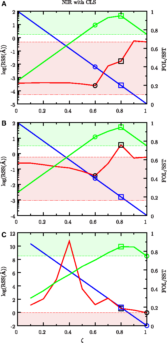
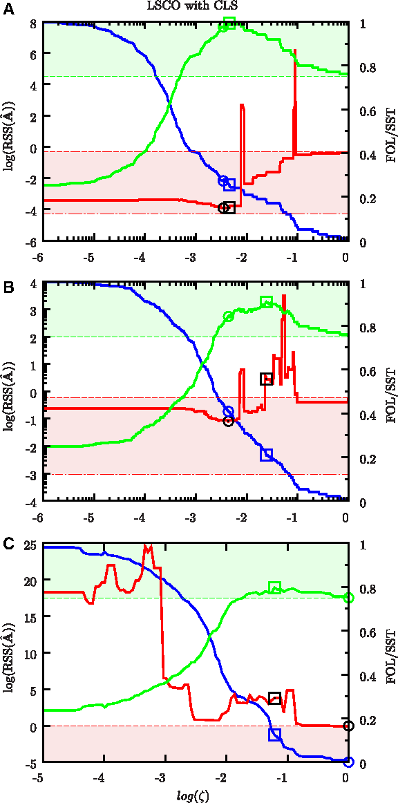
We have investigated the effect of the sparsity coefficient ζ on network inference using three different algorithms: Glmnet, NIR, and LSCO, as well as the performance of the proposed method to identify an optimal ζ value. The inference was done for 1000 ζ values covering the range from a full network to an empty one, and we present the fraction of links (FOL), similarity of signed topology (SST), and residual sum of squares (RSS) of the estimated networks in Figures 1–4. The three data sets differ only in terms of the information content. Therefore, we call the most informative data set with 20 experiments and SNR 35 the “informative data set,” the one with 15 experiments and SNR 7 the “partly informative data set,” and the one with 10 experiments and SNR 1.5 the “uninformative data set.” Using Glmnet and LSCO, it is possible to recover the “true” network for certain ζ values with the informative data set (Figs. 1A and 3A), while none of the three algorithms can recover the “true” network for any ζ value with the other two data sets (Figs. 1–3B and C). It is based on the RSS possible to select the ζ value that gives the best network estimate for the informative and partly informative data sets (Figs. 1–3A and B), but not for the uninformative data set (Figs. 1–3C).
Performance of Glmnet with constrained least squares (CLS) as a function of ζ. Blue curve is the mean fraction of links (FOL), green curve the mean similarity of signed topology (SST), and red curve the mean residual sum of squares (RSS). Informative data with 20 experiments (A), partly informative data with 15 experiments (B) and uninformative data with 10 experiments (C). The best estimates are marked with □ and minimum RSS are marked with○.
Performance of NIR with CLS as a function of ζ. For explanations, see Figure 1.
Performance of LSCO with CLS as a function of ζ. For explanations, see Figure 1.
Performance of Glmnet without CLS as a function of ζ for the informative data (A) and with CLS when all experiments are included in the validation set (B). For explanations, see Figure 1.
All curves represent mean values over all the network estimates obtained by the leave-one-out cross-optimization (LOOCO) for each ζ value. An SST of one implies that all the network estimates contain the same links with same signs as the “true” network, and zero that they are completely different. The shaded green area marks the region in which the network estimates are more similar to the “true” network than an empty network. The lower boundary of this region is in other words defined by the SST of the empty network, and any network estimates with lower SST provide essentially no mechanistic understanding of the system. Previous works have typically used random networks with the correct number of links to define a lower boundary on when an inference method is useful (Menéndez et al., 2010), but we use the empty network, since even random networks with both the correct number of links and fraction of positive and negative ones on average have a lower SST for sufficiently sparse networks like ours (see Supplementary Material). The shaded red area is bounded by the mean RSS for prediction of the responses in the validation set by the empty network A = 0 and the least-squares estimate A = −PY†. The lower boundary is merely included for visual comparison to the least-squares estimate, while any network estimate with a larger RSS than the upper bound essentially is useless for data prediction.
By studying the green SST curve for the three methods in Figures 1–3, it is obvious that an efficient network estimate only is obtained for a narrow range of ζ values. To get a network estimate with an SST within 5% of the best one for the informative data, ζ must be selected within a range of 0.0078 (Glmnet), 0.1 (NIR), and 0.013 (LSCO). This confirms previous reports stating that careful selection of ζ is essential to obtain a network estimate with a structure similar to that of the “true” network (Menéndez et al., 2010).
By comparing the results obtained for the three data sets, the adverse effect of noise and few samples was observed. The SST of the best estimate decreases with decreasing information content for all three methods as expected (Figs. 1–3). Note that each gene will have the same indegree in the estimates given by NIR, while one gene has indegree 4, three genes indegree 3, and the remaining ones indegree 2 in our network (Fig. S1), so NIR cannot for any ζ or data set give an estimate with SST one. This explains why the best NIR estimate for the informative data differs from the “true” network, and why the SST of the best estimate is identical for the informative and partly informative data sets. For all three methods, the RSS of the estimates increases with decreasing information content for most ζ values. The RSS is for all ζ value larger than the RSS of an empty network for the uninformative data set, illustrating that a ζ value giving efficient estimates for mechanistic inference cannot be found based on the RSS when the number of experiments or SNR is too low.
It is well known that regularization introduces a bias in the parameter estimates, and several methods intended to decrease it have been published (Fan and Li, 2001; Fan et al., 2009; Lian, 2009). The effect of this bias on the RSS is best seen in our figures by comparing the red RSS curve in Figure 1A and Figure 4A for the informative data set. The RSS curve generated after re-estimation of the nonzero parameters using constrained least squares (CLS) in Figure 1A has its minimum near the optimal ζ, while the minimum in Figure 4A is located at a smaller ζ value, corresponding to an estimate that has a lower SST than an empty network. In order to find the optimal ζ based on the minimum RSS, this bias must be removed. We have chosen to do such a re-estimation of the nonzero parameters, since many network inference methods with this bias exist, and we want to find a method for selection of ζ that can be wrapped around any network inference method that depends on a sparsity coefficient. In Friedman et al. (2010) and Bonneau et al. (2006), the previouly mentioned one-standard-deviation rule is used in part to compensate for the effect of bias.
Only linearly dependent experiments should be included in the validation data set to avoid predicting the outcome of experiments that the training data set lacks information about. Inclusion of such experiments in general increases the RSS for almost all ζ values and moves the minimum away from the efficient estimate. This is for the informative data set seen by comparing the RSS when all experiments are included in the validation data set used during LOOCO (Fig. 4B) and when only the experiments in \documentclass{aastex}\usepackage{amsbsy}\usepackage{amsfonts}\usepackage{amssymb}\usepackage{bm}\usepackage{mathrsfs}\usepackage{pifont}\usepackage{stmaryrd}\usepackage{textcomp}\usepackage{portland, xspace}\usepackage{amsmath, amsxtra}\pagestyle{empty}\DeclareMathSizes{10}{9}{7}{6}\begin{document}$${\cal V}$$\end{document}Equation (5) are included (Fig 1A). The RSS of the former is at least three orders of magnitude larger in the interesting ζ range.
By combining a selection of linearly dependent experiments and unbiased re-estimation of parameters, it is for sufficiently informative data, based on the RSS of the validation data set, possible to choose a ζ value close to the optimal one, at least for the three inference algorithms that we have investigated here (Figs. 1–3). The proposed ζ selection method hence optimizes the accuracy of the inferred network, with a tendency toward having more false positives than negatives when the “true” network cannot be found. This tendency is best seen for NIR. The “true” network has four links on one row, hence all NIR estimates for a ζ larger than 0.6 lack at least one true link, which increases the RSS and prevents us from finding the optimal ζ. Instead, our method identifies the largest ζ value at which the estimate contains all links present in the “true” network and some false positives.
5. Conclusions
Network estimates that are structurally close to the “true” network are only obtained within a narrow range of ζ values, and estimates that are more different than the empty network are obtained for poor choices. The range of good estimates depends on both the algorithm and data set, which makes data-based selection of ζ imperative. We demonstrate that the ζ value yielding highly accurate network estimates can be determined by minimization of the prediction error in a leave-one-out cross-optimization scheme for data with only 1.5 to 2 times as many experiments as variables.
We also demonstrate the adverse effect of noise and too few samples and how these problems can be detected based on the residual sum of squares becoming larger than for an empty network. Correct selection of ζ requires that noninformative data samples are excluded from the validation set, as well as re-estimation of biased parameters. We therefore include these two steps in the proposed method for ζ optimization. The proposed method can be wrapped around almost any regulatory network inference method and works well for sufficiently informative data, thus improving the workflow from data to network models that provide a better understanding of the biological mechanism.
Footnotes
Disclosure Statement
No competing financial interests exist.
References
1.
BansalM., BelcastroV., Ambesi-ImpiombatoA.et al.2007. How to infer gene networks from expression profiles. Molecular Systems Biology, 3:78.
2.
BonneauR., ReissD.J., ShannonP.et al.2006. The Inferelator: an algorithm for learning parsimonious regulatory networks from systems-biology data sets de novo. Genome Biology, 7:R36.
3.
CandèsE.J., PlanY.2009. Near-ideal model selection by l1 minimization. The Annals of Statistics, 37:2145–2177.
4.
CandesE., WakinM.2008. An introduction to compressive sampling. IEEE Signal Processing Magazine, 25:21–30.
5.
Demir-KavukO., KamadaM., AkutsuT.et al.2011. Prediction using step-wise L1, L2 regularization and feature selection for small data sets with large number of features. BMC Bioinformatics, 12:412.
6.
Di BernardoD., GardnerT.S., CollinsJ.J.2004. Robust identification of large genetic networks. Pacific Symposium on Biocomputing, 497:486–97.
7.
FanJ., LiR.2001. Variable slection via nonconcave penalized likelihood and its oracle properties. Journal of the American Statistical Association, 96:1348–1360.
8.
FanJ., LiR.2006. Statistical challenges with high dimensionality: feature selection in knowledge discovery. Proceedings of the International Congress of Mathematicians. European Mathematical Society: Madrid, Spain.
9.
FanJ., LvJ.2010. A selective overview of variable selection in high dimensional feature space (invited review article)Statistica Sinica, 20:101–148.
10.
FanJ., FengY., WuY.2009. Network exploration via the adaptive LASSO and SCAD penalties. The Annals of Applied Statistics, 3:521–541.
11.
FriedmanJ., HastieT., TibshiraniR.2010. Regularization paths for generalized linear models via coordinate descent. Journal of statistical software, 33:1–22.
12.
GardnerT.S., BernardoD., LorenzD.et al.2003. Inferring genetic networks and identifying compound mode of action via expression profiling. Science, 301:102–105.
13.
HacheH., LehrachH., HerwigR.2009a. Reverse engineering of gene regulatory networks: a comparative study. EURASIP Journal on Bioinformatics & Systems Biology, 617281.
HeF., BallingR., ZengA.-P.2009. Reverse engineering and verification of gene networks: principles, assumptions, and limitations of present methods and future perspectives. Journal of Biotechnology, 144:190–203.
16.
HeckerM., LambeckS., ToepferS.et al.2009. Gene regulatory network inference: data integration in dynamic models-a review. Bio Systems, 96:86–103.
17.
JörnstenR., AbeniusT., KlingT.et al.2011. Network modeling of the transcriptional effects of copy number aberrations in glioblastoma. Molecular Systems Biology, 7:486.
18.
JuliusA., ZavlanosM., BoydS.et al.2009. Genetic network identification using convex programming. IET Systems Biology, 3:155–166.
19.
LianH.2009. Shrinkage tuning parameter selection in precision matrices estimation. Journal of Statistical Planning and Inference, 141:2839–2848.
20.
LorenzD.R., CantorC.R., CollinsJ.J.2009. A network biology approach to aging in yeast. Proceedings of the National Academy of Sciences of the United States of America, 106:1145–1150.
21.
MarbachD., PrillR.J., SchaffterT.et al.2010. Revealing strengths and weaknesses of methods for gene network inference. Proceedings of the National Academy of Sciences of the United States of America, 107:6286–6291.
22.
MendesP., ShaW., YeK.2003. Artificial gene networks for objective comparison of analysis algorithms. Bioinformatics, 19:ii122–ii129.
23.
MenéndezP., KourmpetisY.A.I., ter BraakC.J.F.et al.2010. Gene regulatory networks from multifactorial perturbations using Graphical Lasso: application to the DREAM4 challenge. PloS One, 5:e14147.
24.
NordlingT.E.M., JacobsenE.W.2009. Interampatteness—a generic property of biochemical networks. IET Systems Biology, 3:388.
25.
SchaffterT., MarbachD., FloreanoD.2011. GeneNetWeaver: In silico benchmark generation and performance profiling of network inference methods. Bioinformatics, 27:2263–2270.
26.
StoicaP., SelenY.2004. Model-order selection: a review of information criterion rules. IEEE Signal Processing Magazine, 21:36–47.
27.
ThorssonV., MichaelH.2005. Statistical applications in genetics and molecular biology reverse engineering galactose regulation in yeast through model selection Statistical Applications in Genetics and Molecular. Biology, 4,1.
28.
TibshiraniR.1996. Regression shrinkage and selection via the lasso. Journal of the Royal Statistical Society Series B Methodological, 58:267–288.
29.
WangH., LiR., TsaiC.-L.2007. Tuning parameter selectors for the smoothly clipped absolute deviation method. Biometrika, 94:553–568.
Supplementary Material
Please find the following supplemental material available below.
For Open Access articles published under a Creative Commons License, all supplemental material carries the same license as the article it is associated with.
For non-Open Access articles published, all supplemental material carries a non-exclusive license, and permission requests for re-use of supplemental material or any part of supplemental material shall be sent directly to the copyright owner as specified in the copyright notice associated with the article.