Predicting Protein–Protein Interactions from Multimodal Biological Data Sources via Nonnegative Matrix Tri-Factorization

2.1. Predict new protein interactions via PPI networks

Objective to predict PPIs We first predict protein interactions only using PPI network data. Considering the protein interaction prediction as a matrix completion problem, where the input PPI adjacency matrix X contains missing entries (pairs of proteins whose interactions are yet to be determined), we wish to predict Y, which has full entries (i.e., every element of Y is filled with computed values). Y completes X in the sense that Y _Ω  = X _Ω , or more explicitly, Y _ij  = X _ij , \documentclass{aastex}\usepackage{amsbsy}\usepackage{amsfonts}\usepackage{amssymb}\usepackage{bm}\usepackage{mathrsfs}\usepackage{pifont}\usepackage{stmaryrd}\usepackage{textcomp}\usepackage{portland, xspace}\usepackage{amsmath, amsxtra}\pagestyle{empty}\DeclareMathSizes{10}{9}{7}{6}\begin{document} $$\forall (i , j) \in \Omega$$ \end{document} , where Ω denotes the set of edges where the input adjacency matrix X has known values (the set of interacting edges). Mathematically, the PPI prediction problem can be solved as the following optimization problem: \documentclass{aastex}\usepackage{amsbsy}\usepackage{amsfonts}\usepackage{amssymb}\usepackage{bm}\usepackage{mathrsfs}\usepackage{pifont}\usepackage{stmaryrd}\usepackage{textcomp}\usepackage{portland, xspace}\usepackage{amsmath, amsxtra}\pagestyle{empty}\DeclareMathSizes{10}{9}{7}{6}\begin{document} \begin{align*}\min \limits_{\bf {Y}} \ J_1 = \ \mid\mid {\bf X} - {\bf Y} \mid\mid _ \Omega^2 = \sum \limits_{(i , j) \in \Omega} ({\bf X} - {\bf Y}) _{ij}^2. \tag{2}\end{align*} \end{document}

Due to the low-rank nature of the adjacency matrix as discussed earlier, the completed matrix Y can be factorized and written as Y = HSH ^T , where \documentclass{aastex}\usepackage{amsbsy}\usepackage{amsfonts}\usepackage{amssymb}\usepackage{bm}\usepackage{mathrsfs}\usepackage{pifont}\usepackage{stmaryrd}\usepackage{textcomp}\usepackage{portland, xspace}\usepackage{amsmath, amsxtra}\pagestyle{empty}\DeclareMathSizes{10}{9}{7}{6}\begin{document} $${\bf H} \in {\mathbb R}_{+} ^{n \times k}$$ \end{document} and \documentclass{aastex}\usepackage{amsbsy}\usepackage{amsfonts}\usepackage{amssymb}\usepackage{bm}\usepackage{mathrsfs}\usepackage{pifont}\usepackage{stmaryrd}\usepackage{textcomp}\usepackage{portland, xspace}\usepackage{amsmath, amsxtra}\pagestyle{empty}\DeclareMathSizes{10}{9}{7}{6}\begin{document} $${\bf S} \in {\mathbb R}_{+} ^{k \times k}$$ \end{document} are the factor matrices with nonnegative elements. As a result, Y = HSH ^T can be seen as a low-rank representation of the input matrix X with rank of k ≪ n. Thus, we can rewrite Equation (2) as follows: \documentclass{aastex}\usepackage{amsbsy}\usepackage{amsfonts}\usepackage{amssymb}\usepackage{bm}\usepackage{mathrsfs}\usepackage{pifont}\usepackage{stmaryrd}\usepackage{textcomp}\usepackage{portland, xspace}\usepackage{amsmath, amsxtra}\pagestyle{empty}\DeclareMathSizes{10}{9}{7}{6}\begin{document} \begin{align*}\min \limits_{{\bf H} \geq 0 , {\bf S} \geq 0} \ J_2 = \mid\mid {\bf X} - {\bf HSH}^T \mid\mid _ \Omega^2. \tag{3}\end{align*} \end{document}

Note that, although there exist other low-rank matrix approximation methods, for example, singular value decomposition (SVD), using NMTF as in Equation (3) to constrain the factor matrices H and S to be nonnegative is a natural choice because all the entries of the input PPI adjacency matrix X are positive by definition. Moreover, because of the clustering interpretation of NMTF (Ding et al., 2005, 2006b), other biological data sources can be easily incorporated via manifold regularization as introduced later.

The solution algorithm Different from standard NMTF-based objectives (as in Lee and Seung, 1999; Ding et al., 2005, 2006b; Wang et al., 2011a), which are defined over the whole input nonnegative matrix, the objective in Equation (3) for PPI prediction is defined over a subset of the entries that correspond to known PPIs. Therefore, the solution algorithms to standard NMTF cannot be directly applied to solve Equation (3). To this end, we present an iterative algorithm in Algorithm 1 to solve Equation (3).

The main step of Algorithm 1 is step 4, which solves a symmetric NMF problem (Wang et al., 2011a). Following our earlier publication in Wang et al. (2011a), Equation (5) can be solved by an iterative algorithm with the following updating rules: \documentclass{aastex}\usepackage{amsbsy}\usepackage{amsfonts}\usepackage{amssymb}\usepackage{bm}\usepackage{mathrsfs}\usepackage{pifont}\usepackage{stmaryrd}\usepackage{textcomp}\usepackage{portland, xspace}\usepackage{amsmath, amsxtra}\pagestyle{empty}\DeclareMathSizes{10}{9}{7}{6}\begin{document} \begin{align*} {\bf H} _ {jk} \leftarrow {\bf H} _ {jk} {\left[\frac {{\bf (ZHS)} _ {jk}} {({\bf HSH} ^T {\bf HS}) _ {jk}} \right] ^ {1 / 4}} , \qquad {\bf S} _ {ik} \leftarrow {\bf S} _ {ik} \frac {({\bf H} ^T {\bf ZH}) _ {ik}} {({\bf H} ^T {\bf HSH} ^T {\bf H}) _ {ik}} , \tag {4} \end{align*} \end{document}

where the superscripts are removed for notation brevity. The correctness and convergence of the updating rules in Equation (4) can be rigorously proved as detailed in Wang et al. (2011a). Apparently, Algorithm 1 converts the difficult problem to solve Equation (3) as a series of standard NMTF problems, for which existing algorithms, such as the updating rules in Equation (4), can be used.

Solving Equation (3) by Algorithm 1 for matrix completion, our NMTF approach to predict PPIs is proposed.

The convergence of the solution algorithm Now we prove the following theorem that guarantees the convergence of Algorithm 1.

Theorem 1. Algorithm 1 monotonically decreases the objective value of J₁ in Equation (2) in each iteration.

Proof. First, by definition we have \documentclass{aastex}\usepackage{amsbsy}\usepackage{amsfonts}\usepackage{amssymb}\usepackage{bm}\usepackage{mathrsfs}\usepackage{pifont}\usepackage{stmaryrd}\usepackage{textcomp}\usepackage{portland, xspace}\usepackage{amsmath, amsxtra}\pagestyle{empty}\DeclareMathSizes{10}{9}{7}{6}\begin{document} $${\bf Y}^{(t)} = {\bf Y}_ \Omega^{(t)} + {\bf Y}^{(t)}_M ,$$ \end{document} thus \documentclass{aastex}\usepackage{amsbsy}\usepackage{amsfonts}\usepackage{amssymb}\usepackage{bm}\usepackage{mathrsfs}\usepackage{pifont}\usepackage{stmaryrd}\usepackage{textcomp}\usepackage{portland, xspace}\usepackage{amsmath, amsxtra}\pagestyle{empty}\DeclareMathSizes{10}{9}{7}{6}\begin{document} \begin{align*}\mid \mid {\bf X} - {\bf Y}^{(t)} \mid \mid ^2_ \Omega = \mid \mid ({\bf X}_ \Omega + {\bf Y}^{(t)}_M) - {\bf Y}^{(t)} \mid \mid ^2. \tag{6}\end{align*} \end{document}

Then because Algorithm 1 can be summarized as computing \documentclass{aastex}\usepackage{amsbsy}\usepackage{amsfonts}\usepackage{amssymb}\usepackage{bm}\usepackage{mathrsfs}\usepackage{pifont}\usepackage{stmaryrd}\usepackage{textcomp}\usepackage{portland, xspace}\usepackage{amsmath, amsxtra}\pagestyle{empty}\DeclareMathSizes{10}{9}{7}{6}\begin{document} \begin{align*}\min_{{\bf Y}^{(t + 1)}} \mid \mid ({\bf X}_ \Omega + {\bf Y}_M^{(t)}) - {\bf Y}^{(t + 1)} \mid \mid ^2 , \ \ t = 0 , 1 , {\ldots} \,, \; {\bf Y}_M^{(0)} = 0 , \tag{7}\end{align*} \end{document}

we can derive \documentclass{aastex}\usepackage{amsbsy}\usepackage{amsfonts}\usepackage{amssymb}\usepackage{bm}\usepackage{mathrsfs}\usepackage{pifont}\usepackage{stmaryrd}\usepackage{textcomp}\usepackage{portland, xspace}\usepackage{amsmath, amsxtra}\pagestyle{empty}\DeclareMathSizes{10}{9}{7}{6}\begin{document} \begin{align*}\mid \mid ({\bf X} + {\bf Y}^{(t)}_M) - {\bf Y}^{(t)} \mid \mid ^2 \geq \mid \mid ({\bf X} + {\bf Y}_M^{(t)}) - {\bf Y}^{(t + 1)} \mid \mid ^2. \tag{8}\end{align*} \end{document}

Again, by definition we have \documentclass{aastex}\usepackage{amsbsy}\usepackage{amsfonts}\usepackage{amssymb}\usepackage{bm}\usepackage{mathrsfs}\usepackage{pifont}\usepackage{stmaryrd}\usepackage{textcomp}\usepackage{portland, xspace}\usepackage{amsmath, amsxtra}\pagestyle{empty}\DeclareMathSizes{10}{9}{7}{6}\begin{document} $${\bf Y}^{(t + 1)} = {\bf Y}^{(t + 1)}_ \Omega + {\bf Y}^{(t + 1)}_M$$ \end{document} , thus \documentclass{aastex}\usepackage{amsbsy}\usepackage{amsfonts}\usepackage{amssymb}\usepackage{bm}\usepackage{mathrsfs}\usepackage{pifont}\usepackage{stmaryrd}\usepackage{textcomp}\usepackage{portland, xspace}\usepackage{amsmath, amsxtra}\pagestyle{empty}\DeclareMathSizes{10}{9}{7}{6}\begin{document} \begin{align*} \mid \mid ({\bf X} + {\bf Y}^{(t)}_M) - {\bf Y}^{(t + 1)} \mid \mid ^2 & = \mid \mid ({\bf X} - {\bf Y}^{(t + 1)}) _ \Omega + ({\bf Y}^{(t)} - {\bf Y}^{(t + 1)}) _M \mid \mid ^2 & (9) \\ & = \mid \mid {\bf X} - {\bf Y}^{(t + 1)} \mid \mid ^2_ \Omega + \mid \mid {\bf Y}^{(t)} - {\bf Y}^{(t + 1)} \mid \mid ^2_M \geq \mid \mid {\bf X} - {\bf Y}^{(t + 1)} \mid \mid ^2_ \Omega\end{align*} \end{document}

Combining Equations (6), (8), and (9), we obtain \documentclass{aastex}\usepackage{amsbsy}\usepackage{amsfonts}\usepackage{amssymb}\usepackage{bm}\usepackage{mathrsfs}\usepackage{pifont}\usepackage{stmaryrd}\usepackage{textcomp}\usepackage{portland, xspace}\usepackage{amsmath, amsxtra}\pagestyle{empty}\DeclareMathSizes{10}{9}{7}{6}\begin{document} \begin{align*}\mid \mid {\bf X} - {\bf Y}^{(t)} \mid \mid ^2_ \Omega \geq \mid \mid {\bf X} - {\bf Y}^{(t + 1)} \mid \mid ^2_ \Omega \quad {\rm for} \ t = 0 , 1 , 2 , 3 , {\ldots} \,, \tag{10}\end{align*} \end{document}

which proves the theorem.    ▪

As in Equation (10), the approximation errors, that is, the objective value J₁ in Equation (2), goes down monotonically but remains bigger than zero, i.e., \documentclass{aastex}\usepackage{amsbsy}\usepackage{amsfonts}\usepackage{amssymb}\usepackage{bm}\usepackage{mathrsfs}\usepackage{pifont}\usepackage{stmaryrd}\usepackage{textcomp}\usepackage{portland, xspace}\usepackage{amsmath, amsxtra}\pagestyle{empty}\DeclareMathSizes{10}{9}{7}{6}\begin{document} $$\mid \mid {\bf X} - {\bf Y}^{(0)} \mid \mid ^2_ \Omega \geq \mid \mid {\bf X} - {\bf Y}^{(1)} \mid \mid ^2_ \Omega \geq \mid \mid {\bf X} - {\bf Y}^{(2)} \mid \mid ^2_ \Omega \geq \cdots \geq 0$$ \end{document} , therefore Theorem 1 guarantees the convergence of the algorithm.

2.2. Predict new protein interactions from multimodal biological data

In the last subsection, we introduced how to infer putative protein interactions using only the PPI network data, while in practice we may have other biological data as well, such as protein sequence data (Martin et al., 2005; Shen et al., 2007; Martial et al., 2010), 3D protein structures (Ben-Hur and Noble, 2005; Chen and Liu, 2005; Qiu et al., 2007), and so on. To exploit the useful information contained in the biological data from other sources, in this subsection we further develop the proposed NMTF-based matrix completion approach.

An important reason for the popularity of NMTF in statistical learning lies in its close connection to k-means clustering (Ding et al., 2005, 2006b). Specifically, given a symmetric nonnegative input matrix W, the factor matrix H can be seen as the clustering indications of the vertices (Luo et al., 2009). Therefore, if we have biological data other than PPI networks appearing in form of pairwise similarity, we can incorporate them through manifold regularization (Chung, 1997; Shi and Malik, 2000). Specifically, let \documentclass{aastex}\usepackage{amsbsy}\usepackage{amsfonts}\usepackage{amssymb}\usepackage{bm}\usepackage{mathrsfs}\usepackage{pifont}\usepackage{stmaryrd}\usepackage{textcomp}\usepackage{portland, xspace}\usepackage{amsmath, amsxtra}\pagestyle{empty}\DeclareMathSizes{10}{9}{7}{6}\begin{document} $${\bf W}_{(k)} (0 \leq k \leq K)$$ \end{document} be a set of pairwise similarities constructed from different biological data, an integrated similarity among proteins can be constructed as \documentclass{aastex}\usepackage{amsbsy}\usepackage{amsfonts}\usepackage{amssymb}\usepackage{bm}\usepackage{mathrsfs}\usepackage{pifont}\usepackage{stmaryrd}\usepackage{textcomp}\usepackage{portland, xspace}\usepackage{amsmath, amsxtra}\pagestyle{empty}\DeclareMathSizes{10}{9}{7}{6}\begin{document} $${\bf W} = \sum \nolimits_k \eta_k{\bf W}_{(k)} \ {(\eta_k \geq 0, \sum \nolimits_k \eta_k = 1)}$$ \end{document} where \documentclass{aastex}\usepackage{amsbsy}\usepackage{amsfonts}\usepackage{amssymb}\usepackage{bm}\usepackage{mathrsfs}\usepackage{pifont}\usepackage{stmaryrd}\usepackage{textcomp}\usepackage{portland, xspace}\usepackage{amsmath, amsxtra}\pagestyle{empty}\DeclareMathSizes{10}{9}{7}{6}\begin{document} $$\eta_k$$ \end{document} are parameters to balance the data from different sources. We further develop the objective in Equation (3) as follows: \documentclass{aastex}\usepackage{amsbsy}\usepackage{amsfonts}\usepackage{amssymb}\usepackage{bm}\usepackage{mathrsfs}\usepackage{pifont}\usepackage{stmaryrd}\usepackage{textcomp}\usepackage{portland, xspace}\usepackage{amsmath, amsxtra}\pagestyle{empty}\DeclareMathSizes{10}{9}{7}{6}\begin{document} \begin{align*}\min \limits_{{\bf H} \geq 0 , {\bf S} \geq 0} J_4 = \mid \mid {\bf X} - {\bf HSH}^T \mid \mid _ \Omega^2 + 2 \lambda {\bf tr} ({\bf H}^T ({\bf D} - {\bf W}) {\bf H)} , \qquad s.t. \ {\bf H}^T{\bf D}{\bf H} = I , \tag{11}\end{align*} \end{document}

where D is a diagonal matrix whose diagonal entries D _ii  = ∑ _j W _ij are the degree of the corresponding data points on W, and λ is a parameter to balance the relative importance of the regularization term, which is empirically selected as λ = 0.01 in all our experimental evaluations. Because H can be seen as the “soft” clustering labels (Ding et al., 2005), the second term in Equation (11) enforces the smoothness over the variation of the clustering labels with respect to the underlying manifold described by W (Cai et al., 2008; Gu and Zhou, 2009), by which additional biological data sources are incorporated.

Equation (11) takes a similar form to Equation (3), which, again, is not a standard NMTF problem. We use Algorithm 1 to solve it by replacing step 4 to minimize the following objective: \documentclass{aastex}\usepackage{amsbsy}\usepackage{amsfonts}\usepackage{amssymb}\usepackage{bm}\usepackage{mathrsfs}\usepackage{pifont}\usepackage{stmaryrd}\usepackage{textcomp}\usepackage{portland, xspace}\usepackage{amsmath, amsxtra}\pagestyle{empty}\DeclareMathSizes{10}{9}{7}{6}\begin{document} \begin{align*}J_4 = \mid \mid {\bf Z} - {\bf HSH}^T \mid \mid ^2 + 2 \lambda{\bf tr} ({\bf H}^T ({\bf D} - {\bf W}) {\bf H}) , \qquad s.t. \ {\bf H} \geq 0 , {\bf S} \geq 0 , {\bf H}^T{\bf DH} = I , \tag{12}\end{align*} \end{document}

which can be solved using the following updating rules: \documentclass{aastex}\usepackage{amsbsy}\usepackage{amsfonts}\usepackage{amssymb}\usepackage{bm}\usepackage{mathrsfs}\usepackage{pifont}\usepackage{stmaryrd}\usepackage{textcomp}\usepackage{portland, xspace}\usepackage{amsmath, amsxtra}\pagestyle{empty}\DeclareMathSizes{10}{9}{7}{6}\begin{document} \begin{align*} {\bf H} _ {ik} \leftarrow {\bf H} _ {ik} \left[\frac {({\bf ZHS} + \lambda {\bf WH}) _ {ik}} {({\bf HSH} ^T {\bf HS} + {\bf DH} {\Lambda}) _ {ik}} \right] ^ \frac {1} {4} , \qquad {\bf S} _ {ik} \leftarrow {\bf S} _ {ik} \left[\frac {({\bf H} ^T {\bf ZH}) _ {ik}} {({\bf H} ^T {\bf HSH} ^T {\bf H}) _ {ik}} \right] ^ \frac {1} {2} , \tag {13} \end{align*} \end{document}

where Λ is the Lagrangian multiplier for the constraint H ^T DH = I, and its value is given by Λ =H ^T XHS − H ^T HSH ^T HS + λH ^T WH. The rigorous proof of the correctness and the convergence of the iteration procedures in Equation (13) can be found in our earlier publication in Wang et al. (2011e).

Note that, the objective in Equation (12) is different from the objectives of many existing related works (Cai et al., 2008; Gu and Zhou, 2009) using NMF in that the orthogonality H ^T DH = I is enforced. This is important because the second term of Equation (12) can be written as \documentclass{aastex}\usepackage{amsbsy}\usepackage{amsfonts}\usepackage{amssymb}\usepackage{bm}\usepackage{mathrsfs}\usepackage{pifont}\usepackage{stmaryrd}\usepackage{textcomp}\usepackage{portland, xspace}\usepackage{amsmath, amsxtra}\pagestyle{empty}\DeclareMathSizes{10}{9}{7}{6}\begin{document} $${\bf tr} ({\bf H}^T ({\bf D} - {\bf W}) {\bf H}) = \sum\nolimits_{k = 1}^K h_k^T ({\bf D} - {\bf W}) h_k$$ \end{document} . Without the orthogonality constraint, different columns become independent of each other, thereby reaching the same minimum with same solution, that is, \documentclass{aastex}\usepackage{amsbsy}\usepackage{amsfonts}\usepackage{amssymb}\usepackage{bm}\usepackage{mathrsfs}\usepackage{pifont}\usepackage{stmaryrd}\usepackage{textcomp}\usepackage{portland, xspace}\usepackage{amsmath, amsxtra}\pagestyle{empty}\DeclareMathSizes{10}{9}{7}{6}\begin{document} $$h_1^* = \cdots = h_k^*$$ \end{document} . When λ is not small, degenerate solution will be obtained and the approximation of Z by HSH ^T is degraded. We refer interested readers to Wang et al. (2011e) for more detailed discussions on the importance and effectiveness of enforcing orthogonality constraints in manifold regularized NMTF.

Solving Equation (11) for matrix completion, our regularized non-negative matrix tri-factorization (R-NMTF) approach for PPI prediction is proposed, which is able to utilize both PPI network data as well as other biological data.

4.1. Improved prediction capability in cross-validation

We first evaluate the proposed methods and compare their prediction capabilities against three most recent PPI prediction methods.

(1) Tensor product pairwise kernel (TPPK) method (Ben-Hur and Noble, 2005): This method builds a kernel for pairwise objects. In order for a fair comparison, protein sequence and protein interaction network topology are used for kernel construction. PPI prediction is then carried out by the ranking scores for noninteracting protein pairs yielded by an SVM on the resulted score.

where \documentclass{aastex}\usepackage{amsbsy}\usepackage{amsfonts}\usepackage{amssymb}\usepackage{bm}\usepackage{mathrsfs}\usepackage{pifont}\usepackage{stmaryrd}\usepackage{textcomp}\usepackage{portland, xspace}\usepackage{amsmath, amsxtra}\pagestyle{empty}\DeclareMathSizes{10}{9}{7}{6}\begin{document} $${\cal N}_k (x_i)$$ \end{document} is the set of k-nearest neighbors of x_i, and d (·,·) is distance function built from a kernel by \documentclass{aastex}\usepackage{amsbsy}\usepackage{amsfonts}\usepackage{amssymb}\usepackage{bm}\usepackage{mathrsfs}\usepackage{pifont}\usepackage{stmaryrd}\usepackage{textcomp}\usepackage{portland, xspace}\usepackage{amsmath, amsxtra}\pagestyle{empty}\DeclareMathSizes{10}{9}{7}{6}\begin{document} $$d (x_i , x_j) = \sqrt{{\cal K} (x_i , x_i) - 2{\cal K} (x_i , x_j) + {\cal K} (x_j , x_j)}$$ \end{document} . In our evaluations, we use the mismatch kernel for protein sequence data.

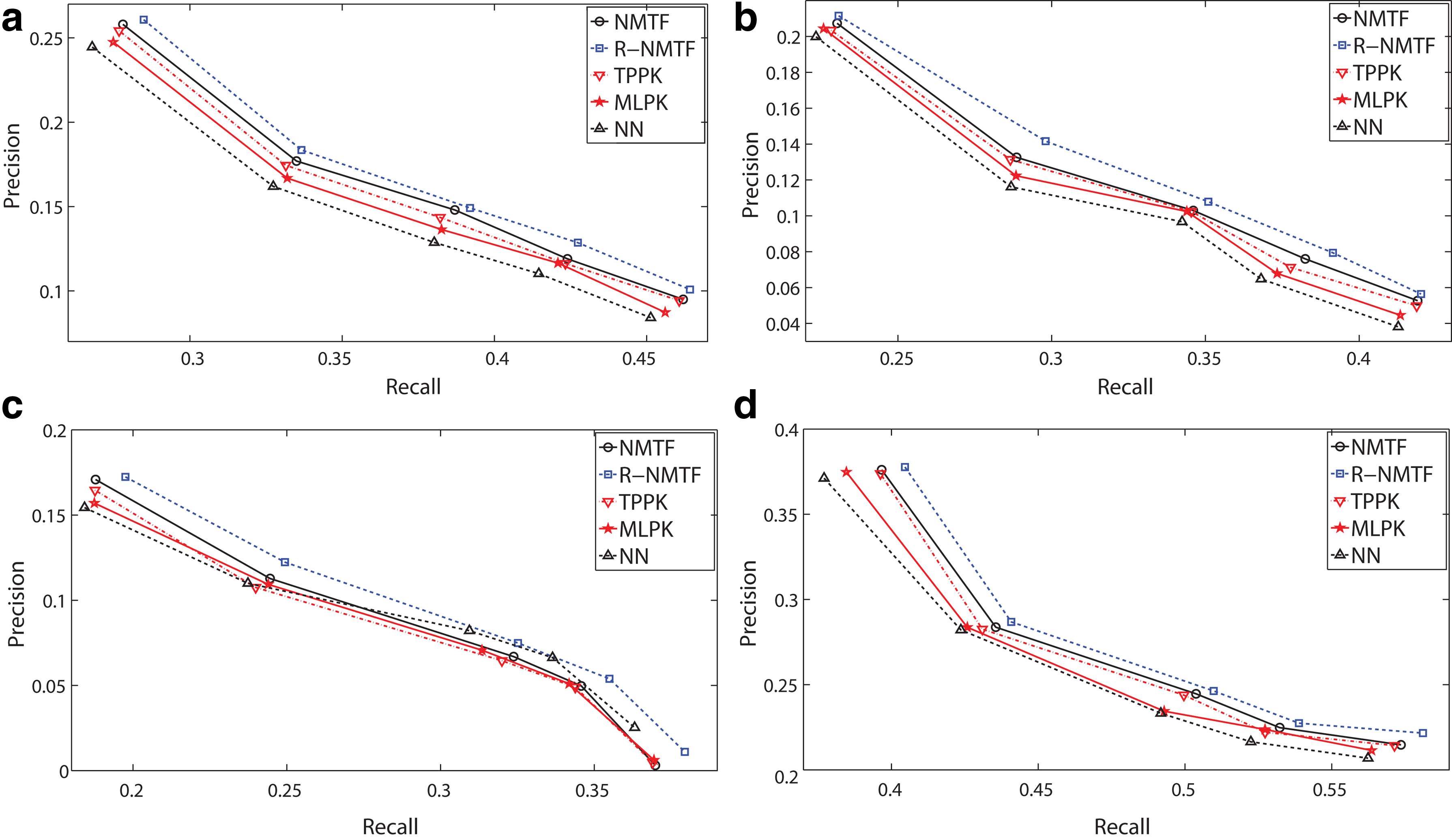
Experimental procedures For each method, we perform 20-fold cross-validation as follows. For each trial, we remove 5% known edges (PPIs) from the input graph and try to recover them using the remaining graph, which is repeated by 10 times. The average results over the 10 trials on every species are reported in Figure 2. During each trial, an internal five-fold cross validation is performed for parameter selection. For our NMTF and R-NMTF methods, the parameter is the rank k of the factor matrices H and S. For TPPK and MLPK methods, we use the Gaussian kernel, therefore the parameters are the two regularization parameters. For NN method, we select the k of NN from {1, 2, 3, 5, 10, 15}, which is the same as in Martial et al. (2010). We fine-tune the parameters for best prediction precision for all the compared methods.

OPEN IN VIEWER

FIG. 2.

Precision-recall curves by 20-fold cross-validation on four species by the compared PPI prediction methods. NMFT, nonnegative matrix tri-factorization; R-NMTF, regularized nonnegative matrix tri-factorization; TPPK, tensor product pairwise kernel method; MLPK, metric learning pairwise kernel method; NN, nearest neighbor.

Results Because all compared methods produce a list of ranking scores for noninteracting protein pairs, we employ precision-recall curves to measure the prediction performance. We compute the precisions and recalls when picking up a range of top k noninteracting protein pairs as predictions and average them over the 10 trials. The resulted precision-recall curves of four species are reported in Figure 2. From the results, we can see that both proposed methods, NMTF and R-NMTF, consistently outperform comparable methods, sometimes very significantly. In addition, the prediction performances of R-NMTF method are always better than those of NMTF method, which is consistent with our previous theoretical analysis in that multimodal biological data, i.e., protein interaction network plus protein sequence data, offer enhanced prediction performance. We also observe that the TPPK method achieves similar performances to the proposed NMTF method for D. melanogaster and C. elegans species. However, our NMTF method uses only protein interaction network data, while TPPK method exploits both network data and sequence data.

A more careful analysis on the prediction results shows that the noninteracting protein pairs (including the noninteracting protein paris in the original PPI graphs and those removed due to cross-validation) with high ranking scores identified by the proposed methods typically exhibit high similarities in their functional roles. In Table 2, we list the predicted protein pairs with top 10 highest ranking scores by R-NMTF method on S. cerevisiae species, in which the biological functions of all protein pairs are very similar to each other. For example, “PHO91” works as “Low-affinity phosphate transporter of the vacuolar membrane,” which is also the main functional role of its putative interacting partner “PHO90.” Moreover, both of them have functionalities of “transcription independent of Pi and Pho4p activity” and “overexpression results in vigorous growth.” These observations clearly demonstrate that these two proteins are functionally related and tend to interact with each other, which provides concrete evidence to support that the predicted protein interactions by the proposed R-NMTF are biologically meaningful.

Note that, in our empirical studies, we only use one additional data source (i.e., protein sequence data) for the purpose of demonstration. In practice, more biological data, when available, could be incorporated through a proper kernel construction under the R-NMTF prediction framework to achieve better prediction results.

4.2. Conserved functional similarity of predicted new protein interactions

It is generally believed that interacting protein pairs tend to have similar functional roles. We test this hypothesis by evaluating the function similarities between our predicted interacting proteins on S. cerevisiae species. We use the Resnik score (Resnik, 1995) on the GO annotation system to measure the functional similarities between protein pairs.

Specifically, given a term t in GO, its information content is quantified as −log, where the probability of the term is taken to be its frequency among annotations to all GO terms. If a term t is annotated to a protein, it must be annotated with all the ancestors of the term t. Therefore, the higher the term is located in the GO hierarchy, the less its information content. In the case of GO, a term might have multiple parent terms, so that a pair of terms might have more than one path of common ancestors. Denoting the set of all common-ancestor terms of t₁ and t₂ as A(t₁, t₂) we define the similarity between two terms, t₁ and t₂, as sim \documentclass{aastex}\usepackage{amsbsy}\usepackage{amsfonts}\usepackage{amssymb}\usepackage{bm}\usepackage{mathrsfs}\usepackage{pifont}\usepackage{stmaryrd}\usepackage{textcomp}\usepackage{portland, xspace}\usepackage{amsmath, amsxtra}\pagestyle{empty}\DeclareMathSizes{10}{9}{7}{6}\begin{document} $$ (t_1, t_2) = \max \nolimits_{a \in A} (t_1, t_2) - \log p(a) $$ \end{document} . Because an individual protein could have multiple functions, we compute the similarity of two proteins, p₁ and p₂, by matching each function of p₁ to its most similar function of p₂, and the average is taken over all such pairs of functions as sim \documentclass{aastex}\usepackage{amsbsy}\usepackage{amsfonts}\usepackage{amssymb}\usepackage{bm}\usepackage{mathrsfs}\usepackage{pifont}\usepackage{stmaryrd}\usepackage{textcomp}\usepackage{portland, xspace}\usepackage{amsmath, amsxtra}\pagestyle{empty}\DeclareMathSizes{10}{9}{7}{6}\begin{document} $$(p_1 \rightarrow p_2) = {\rm avg} \left[\sum{_{s \in p_1}} \max \nolimits_{{t \in p_2}} \ {\rm sim} (s , t) \right]$$ \end{document} . As this measurement is not symmetric with respect to p₁ and p₂, the final semantic similarity between the two proteins is defined as sim \documentclass{aastex}\usepackage{amsbsy}\usepackage{amsfonts}\usepackage{amssymb}\usepackage{bm}\usepackage{mathrsfs}\usepackage{pifont}\usepackage{stmaryrd}\usepackage{textcomp}\usepackage{portland, xspace}\usepackage{amsmath, amsxtra}\pagestyle{empty}\DeclareMathSizes{10}{9}{7}{6}\begin{document} $$(p_1 , p_2) = \frac {1} {2} \times \left[{\rm sim} \ (p_1 \rightarrow p_2) + {\rm sim} \ (p_2 \rightarrow p_1) \right]$$ \end{document} .

The average Resnik scores of known interacting protein pairs, noninteracting protein pairs, and predicted putative interacting protein pairs by the proposed NMTF and R-NMTF methods are reported in Table 3, from which we have the following observations.

First, the average Resnik score of known interacting protein pairs is higher than that of noninteracting protein pairs, which is consistent with the aforementioned assumption that the interacting protein pairs have more similar biological functions than those not interacting.

Second, the average Resnik score of the predicted putative interacting protein pairs by the proposed NMTF and R-NMTF methods are close to that of known interacting protein pairs. Namely, the proteins in the predicted PPIs are highly functionally similar, which confirms the correctness of the proposed methods from protein function similarity perspective.

Last, but not least, the predicted protein interactions by R-NMTF method have higher semantic score than those by NMTF method. Therefore, prediction by R-NMTF method using multimodal biological data sources is more advantageous than that by NMTF method using only one data source.

4.3. Capability to predict new protein interactions

The ultimate goal of computational methods to predict protein interactions is to discover new interacting protein pairs that can be served as potential targets for experimental screening. Therefore, we predict protein interactions on S. cerevisiae species by the proposed R-NMTF method on the PPI graph using BioGRID data of version 2.0.56 (published on August 31, 2009).

We examine the prediction results and find that among the top 200 putative PPIs predicted by our R-NMTF method, 87 protein pairs are consistent with other evidence (i.e., they are verified by experimental results and appear in recent published literatures). For example, protein “BNI1” and protein “CTF3” are not documented as a PPI in BioGRID data of version 2.0.56 but predicted to be interacting by our method. By a careful document survey, we notice that the experimental supporting document to this protein pair only appears in early 2010 (Vizeacoumar et al., 2010). This result firmly confirms the effectiveness of our method in predicting new protein interactions. Other predicted putative protein pairs together with the PubMed document IDs for their supporting literatures are listed in Appendix Table 5. Most them are also incorporated in the most recent BioGRID data of version 3.1.69 (published on September 30, 2010). The high overlaps between our predictions and the results in existing literature give a solid support of the usefulness of the proposed method.

4.4. Improved protein function prediction using predicted PPI networks

Protein interaction networks are broadly used in various biological applications, whose performances are inevitably determined by the quality input PPI graphs. Therefore, we assess the quality of predicted PPI networks in protein function prediction on S. cerevisiae species.

We predict protein functions on the original PPI graph constructed from the BioGRID database, the PPI graph filled by the top 1000 putative interacting protein pairs predicted by NMTF method, and that by R-NMTF method. We make predictions using the following three benchmark graph-based protein function prediction methods:

(1) Majority voting (MV) (Schwikowski et al., 2000) method: This method assigns functions to a protein via its connecting neighbors in certain ranges.

We implement these methods following the details in the original literatures. Because FF method produces a ranking list of predicted protein functions, we select a threshold such that the prediction precision is maximized. Five-fold cross-validation is performed to predict the functions in “biological process” of GO. The average prediction precision over all test functions and five trials of cross-validation of the involved methods on different PPI graphs are reported in Table 4.

The results in Table 4 show that the function prediction performance for all three methods are improved when the predicted PPI graphs are used. Such results experimentally prove that the predicted PPI graphs have higher quality than the original one, which demonstrates that the filled putative protein interactions by the proposed methods are largely biologically meaningful. Thus, we can tentatively conclude that the proposed NMTF and R-NMTF indeed can improve the protein interaction networks. Again, multimodal biological data sources based R-NMTF method is better than single data source-based NMTF method.

6.1. Predicted new protein interactions with highest-ranking scores by R-NMTF method

In Table 5, we list a subset (87 out of 200) of the predicted putative protein interactions with highest ranking scores on the original S. cerevisiae PPI graph by the proposed R-NMTF method. These protein pairs are already discovered to be interacting in existing literatures. The document ID in PubMed of the supporting literatures are listed in the third column of Table 5.

References

1.
AloyP., CeulemansH., StarkA.et al.2003. The relationship between sequence and interaction divergence in proteins. J. Mol. Biol., 332:989–998.
2.
AshburnerM., BallC., BlakeJ.et al.2000. Gene ontology: tool for the unification of biology. Nat. Genet., 25:25–29.
3.
BarkerD., PagelM.2005. Predicting functional gene-links from phylogenetic-statistical analyses of whole genomes. PLoS Comp. Biol., 1:24–31.
4.
Ben-HurA., NobleW.2005. Kernel methods for predicting protein–protein interactions. Bioinformatics, 21:i38.
BowersP., CokusS., EisenbergD.et al.2004a. Use of logic relationships to decipher protein network organization. Science, 306:2246.
7.
BowersP., O'ConnorB., CokusS.et al.2005. Utilizing logical relationships in genomic data to decipher cellular processes. FEBS Journal, 272:5110–5118.
8.
BowersP., PellegriniM., ThompsonM.et al.2004b. Prolinks: a database of protein functional linkages derived from coevolution. Genome Biol., 5:R35.
9.
CaiD., HeX., WuX.et al.2008. Non-negative matrix factorization on manifold. In Proceedings of the 2008 Eighth IEEE International Conference on Data Mining, 63–72.
10.
CandèsE., PlanY.2009. Matrix completion with noise. Proceedings of the IEEE.
DaiO., PrasadN.2010. Low-rank matrix completion for inference of protein-protein interaction networks. In AIP Conference Proceedings. 1281:1531.
16.
DingC., HeX., SimonH.2005. On the equivalence of nonnegative matrix factorization and spectral clustering. Proc. SIAM Data Mining Conf, 606–610.
17.
DingC., LiT., JordanM.2006a. Convex and semi-nonnegative matrix factorizations for clustering and low-dimension representation. Technical Report LBNL-60428. Lawrence Berkeley National Laboratory.
18.
DingC., LiT., PengW.et al.2006b. Orthogonal nonnegative matrix t-factorizations for clustering. Proceedings of the 12th ACM SIGKDD international conference on knowledge discovery and data mining, 126–135.
19.
EnrightA., IliopoulosI., KyrpidesN.et al.1999. Protein interaction maps for complete genomes based on gene fusion events. Nature, 402:86–90.
20.
ErmolaevaM., WhiteO., SalzbergS.2001. Prediction of operons in microbial genomes. Nucleic Acids Res., 29:1216.
21.
GohC., BoganA., JoachimiakM.et al.2000. Co-evolution of proteins with their interaction partners1. J. Mol. Biol., 299:283–293.
22.
GuQ., ZhouJ.2009. Co-clustering on manifolds. Proceedings of the 15th ACM SIGKDD international conference on knowledge discovery and data mining, 359–368.
23.
HoY., GruhlerA., HeilbutA.et al.2002. Systematic identification of protein complexes in Saccharomyces cerevisiae by mass spectrometry. Nature, 415:180–183.
24.
ItoT., TashiroK., MutaS.et al.2000. Toward a protein–protein interaction map of the budding yeast: a comprehensive system to examine two-hybrid interactions in all possible combinations between the yeast proteins. Proceedings of the National Academy of Sciences of the United States of America, 97:1143.
25.
JansenR., YuH., GreenbaumD.et al.2003. A Bayesian networks approach for predicting protein–protein interactions from genomic data. Science, 302:449.
26.
JothiR., CherukuriP., TasneemA.et al.2006. Co-evolutionary analysis of domains in interacting proteins reveals insights into domain-domain interactions mediating protein–protein interactions. J. Mol. Biol., 362:861–875.
27.
LeeD., SeungH.1999. Learning the parts of objects by non-negative matrix factorization. Nature, 401:788–791.
28.
LeslieC., EskinE., WestonJ.et al.2003. Mismatch string kernels for SVM protein classification. Adv Neural Inf Process Syst., 1441–1448.
29.
LittlerS., HubbardS.2005. Conservation of orientation and sequence in protein domain-domain interactions. J. Mol. Biol., 345:1265–1279.
30.
LuoD., DingC., HuangH.et al.2009. Non-negative laplacian embedding. In 2009 Ninth IEEE International Conference on Data Mining, 337–346.
31.
MarcotteC., MarcotteE.2002. Predicting functional linkages from gene fusions with confidence. Applied Bioinformatics, 1:93–100.
32.
MarcotteE., PellegriniM., NgH.et al.1999. Detecting protein function and protein–protein interactions from genome sequences. Science, 285:751.
33.
MartialH., MichaelR., Jean-PhilippeV.et al.2010. Large-scale prediction of protein–protein interactions from structures. BMC Bioinformatics, 11.
Moreno-HagelsiebG., Collado-VidesJ.2002. A powerful non-homology method for the prediction of operons in prokaryotes. Bioinformatics, 18:S329.
36.
NabievaE., JimK., AgarwalA.et al.2005. Whole-proteome prediction of protein function via graph-theoretic analysis of interaction maps. Bioinformatics, 21:i302.
37.
NoorenI., ThorntonJ.2003. Structural characterisation and functional significance of transient protein–protein interactions. J. Mol. Biol., 325:991–1018.
38.
PagelP., WongP., FrishmanD.2004. A domain interaction map based on phylogenetic profiling. J. Mol. Biol., 344:1331–1346.
39.
PanchenkoA., WolfY., PanchenkoL.et al.2005. Evolutionary plasticity of protein families: coupling between sequence and structure variation. Proteins: Structure, Function, and Bioinformatics, 61:535–544.
40.
QiY., Klein-SeetharamanJ., Bar-JosephZ.2005. Random forest similarity for protein–protein interaction prediction from multiple sources. Pac Symp Biocomput., 10:531–542.
41.
QiuJ., HueM., Ben-HurA.et al.2007. A structural alignment kernel for protein structures. Bioinformatics, 23:1090.
42.
RamaniA., MarcotteE.2003. Exploiting the co-evolution of interacting proteins to discover interaction specificity. J. Mol. Biol., 327:273–284.
43.
ResnikP.1995. Using information content to evaluate semantic similarity in a taxonomy. Arxiv preprint cmp-lg/9511007.
44.
SalgadoH., Moreno-HagelsiebG., SmithT.et al.2000. Operons in Escherichia coli: genomic analyses and predictions. Proceedings of the National Academy of Sciences of the United States of America, 97:6652.
45.
SchwikowskiB., UetzP., FieldsS.2000. A network of protein–protein interactions in yeast. Nat. Biotech., 18:1257–1261.
46.
ShenJ., ZhangJ., LuoX.et al.2007. Predicting protein–protein interactions based only on sequences information. Proceedings of the National Academy of Sciences, 104:4337.
47.
ShiJ., MalikJ.2000. Normalized cuts and image segmentation. IEEE. Trans. on Pattern Analysis and Machine Intelligence, 22:888–905.
48.
ShoemakerB., PanchenkoA.2007a. Deciphering protein–protein interactions. Part I. Experimental techniques and databases. PLoS Comp. Biol., 3:337–334.
49.
ShoemakerB., PanchenkoA.2007b. Deciphering protein–protein interactions. Part II. Computational methods to predict protein and domain interaction partners. PLoS Comp. Biol., 3:595–601.
50.
StarkC., BreitkreutzB., RegulyT.et al.2006. BioGRID: a general repository for interaction datasets. Nucleic Acids Res., 34:D535.
51.
StrongM., MallickP., PellegriniM.et al.2003. Inference of protein function and protein linkages in Mycobacterium tuberculosis based on prokaryotic genome organization: a combined computational approach. Genome Biol., 4:R59.
52.
TeichmannS.2002. The constraints protein-protein interactions place on sequence divergence. J. Mol. Biol., 324:399–407.
53.
ValdarW., ThorntonJ.2001. Protein-protein interfaces: analysis of amino acid conservation in homodimers. Proteins: Structure, Function, and Bioinformatics, 42:108–124.
54.
VazquezA., FlamminiA., MaritanA.et al.2003. Global protein function prediction from protein-protein interaction networks. Nat. biotechnology, 21:697–700.
55.
VizeacoumarF., Van DykN., VizeacoumarF.et al.2010. Integrating high-throughput genetic interaction mapping and high-content screening to explore yeast spindle morphogenesis. J. Cell. Biol., 188:69.
56.
WangH., HuangH., DingH.2011a. Simultaneous clustering of multi-type relational data via symmetric nonnegative matrix tri-factorization. In The 20th ACM Conference on Information and Knowledge Management.
57.
WangH., HuangH., NieF.et al.2011b. Cross-language web page classification via dual knowledge transfer using nonnegative matrix tri-factorization. In Proceedings of the 34th international ACM SIGIR conference (ACM SIGIR 2011), 933–942.
58.
WangH., NieF., HuangH., DingC.2011c. Dyadic transfer learning for cross-domain image classification. In 2011 IEEE International Conference on Computer Vision (IEEE ICCV 2011), 551–556.
59.
WangH., NieF., HuangH.et al.2011d. Fast nonnegative matrix tri-factorization for large-scale data co-clustering. In Twenty-Second International Joint Conference on Artificial Intelligence (IJCAI 2011).
60.
WangH., NieF., HuangH.et al.2011e. Nonnegative matrix tri-factorization based high-order co-clustering and its fast implementation. In 2011 Eleventh IEEE International Conference on Data Mining.
61.
YanaiI., DertiA., DeLisiC.2001. Genes linked by fusion events are generally of the same functional category: a systematic analysis of 30 microbial genomes. Proceedings of the National Academy of Sciences of the United States of America, 98:7940.
62.
ZhangL., WongS., KingO.et al.2004. Predicting co-complexed protein pairs using genomic and proteomic data integration. BMC Bioinformatics, 5:38.