On Topological RNA Interaction Structures

Abstract

Recently a folding algorithm of topological RNA pseudoknot structures was presented in Reidys et al. (2011). This algorithm folds single-stranded γ-structures, that is, RNA structures composed by distinct motifs of bounded topological genus. In this article, we set the theoretical foundations for the folding of the two backbone analogues of γ structures: the RNA γ-interaction structures. These are RNA–RNA interaction structures that are constructed by a finite number of building blocks over two backbones having genus at most γ. Combinatorial properties of γ-interaction structures are of practical interest since they have direct implications for the folding of topological interaction structures. We compute the generating function of γ-interaction structures and show that it is algebraic, which implies that the numbers of interaction structures can be computed recursively. We obtain simple asymptotic formulas for 0- and 1-interaction structures. The simplest class of interaction structures are the 0-interaction structures, which represent the two backbone analogues of secondary structures.

1. Introduction

The fact that nucleic acids are capable of recognizing other nucleic acids with very high specificity by means of complementary base pairing is the basis of many basic laboratory techniques, starting with designed RNA and DNA primers. Not surprisingly, direct interactions of nucleic acids are also an important mechanism in gene regulation. The most prominent examples are certainly microRNAs and siRNAs, which bind their targets by forming more or less perfect helical regions. More complex structures of the RNA–RNA binding are the rule for snoRNAs and, in particular, for a wide variety of small bacterial sRNAs. RNA–RNA binding is not limited to small structured RNAs addressing protein-coding mRNAs. In many cases, the regulatory effect of bacterial sRNA–mRNA interactions can be understood in terms of the underlying interaction structure. Namely, depending on the location of the binding site, conformational changes can lead to the sequestration or exposure of the Shine-Dalgarno sequence and hence disable or enable translation.

Interactions between nucleic acids can be understood to a good approximation at the level of secondary structures (patterns of base pairs) or extended secondary structures. From a technical point of view, therefore, the analysis, prediction, and comparison of RNA–RNA and RNA–DNA interaction structures are formalized as a suite of related combinatorial (optimization) problems that make genome-wide studies computationally feasible and set RNA bioinformatics apart from other areas of structural biology in which three-dimensional shapes and atomic detail cannot be neglected as easily. For instance, the interaction of eukaryotic miRNA with their targets, in addition to bacterial sRNA and mRNA—plant miRNA/mRNA and animal miRNA/mRNA interactions—may require a detailed 3D analysis by means of non-canonical base pairs. Despite this favorable starting point and the success of the combinatorial approach to structures of individual nucleic acid molecules, we nevertheless lack both theoretical insights and practical predictive power in the realm of interactions.

The simplest approach for folding RNA–RNA interaction structures concatenates two (or more) interacting sequences, one after another, remembering the specific merge point (cut-point), and then employs the standard secondary structure–folding algorithm on a single strand. This approach falls short of predicting many genuine features, such as kissing-hairpin loops. The paradigm of concatenation has also been generalized to include cross-serial interactions (Rivas and Eddy, 1999). The resulting model, however, still does not generate all relevant interaction structures (Busch et al., 2008). An alternative is to neglect any internal base pairings in either strand, that is, to compute the minimum free energy (MFE) secondary structure of hybridization of otherwise unstructured RNAs. This ansatz (Busch et al., 2008; Mückstein et al., 2006, 2008) restricts interactions to a single interval that remains unpaired in the secondary structure for each partner.

A different approach was taken independently by Alkan et al. (2006) and Pervouchine (2004), who proposed MFE folding algorithms for predicting the AP-structure of two interacting RNA molecules. In this model, the intramolecular structures of each partner are pseudoknot-free, the intermolecular binding pairs are noncrossing, and there is an ad hoc exclusion of so-called “zig-zag” motifs. The RNA–RNA interaction structures of Alkan et al. (2006), Bernhart et al. (2006), Hofacker et al. (1994), and Huang et al. (2010) have the following features: (a) When drawing the two backbones on top of each other, all base pairs are noncrossing, that is, no pseudoknots formed by internal or external arcs are allowed, and (b) zig-zag motifs are disallowed.

The abundance of RNA–RNA interactions is motivation to identify the analogue of RNA secondary structures. As in the case of RNA structures over one backbone, the key issue is to identify and analyze a suited filtration of RNA–RNA interaction structures. The filtration presented here is based on the topological genus of certain structural motifs and allows for a polynomial time folding of the accordingly filtered interaction structures. In contrast to a pure genus filtration, the structures presented here have arbitrarily high genus; it is only their motifs that are genus constrainted. The interaction structures considered here allow, in fact, for arbitrary composition and nesting of these genus-constrained motifs.

The classification and expansion of pseudoknotted RNA structures in terms of the topological genus of an associated fatgraph or double line graph were first proposed in Bon et al. (2008) and Orland and Zee (2002), although fatgraphs were applied to RNA secondary structures already by Penner (2004) and Penner and Waterman (1993). The first enumerative results initiated in Orland and Zee (2002) and Vernizzi and Orland (2005) are an application of matrix models from theoretical physics. Genus as well as other topological invariants of fatgraphs were introduced and studied as descriptors of proteins in Penner et al. (2010).

In Reidys et al. (2011), RNA γ-structures were introduced. The idea of γ-structures is to consider RNA structures obtained by building blocks, having topological genus at most γ. From this point of view, RNA secondary structures can be seen to be obtained by the building block that is simply an arc by means of concatenation and nesting. Accordingly, secondary structures are equivalent to 0 structures over one backbone. We call these blocks, in the case of genus, greater or equal to one irreducible shadow. In this sense, topological genus controls the complexity of the cross-serial interactions expressed in these irreducible shadows. In Reidys et al. (2011), but already implicit in Zagier (1995), it was proven that for any genus, there are only finitely many irreducible shadows.

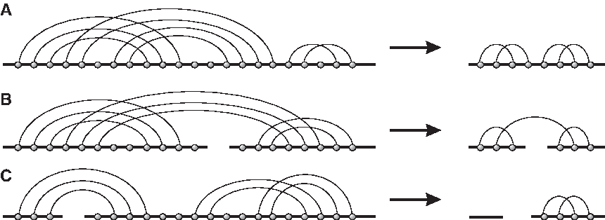
RNA interaction structures of fixed topological genus (Andersen et al., 2012) have, as their one backbone counterpart, only finitely many irreducible shadows. Following the identification of these, Andersen et al. (2012) develops the concept of RNA γ-interaction structures. Note that the genus of γ-interaction structures is not fixed. For the simplest class, the 0-interaction structures, we already have an unambiguous grammar (Andersen et al., 2012) (Fig. 1). While genus zero structures are exactly RNA secondary structures that only contain noncrossing arcs, genus zero interaction structures exhibit crossings (Fig. 1). Such cross-serial interactions, however, can only occur for exterior arcs, that is, arcs that connect the two backbones.

FIG. 1.

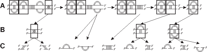
An unambiguous grammar of 0-interaction structures; see Andersen et al. (2012) for details.

The idea of topological RNA interaction structures is a topic of considerable practical interest, since RNA interaction structures that do not belong to the AP structure exist. For instance, the integral RNA (hTER) of the human telomerase ribonucleoprotein has a conserved secondary structure that contains a potential pseudoknot (Ly et al., 2003). There is evidence that the two conserved complementary sequences of one stem of the hTER pseudoknot domain can pair intermolecularly in vitro, and that formation of this stem as part of a novel “transpseudoknot” is required for the telomerase to be active in its dimeric form (Fig. 2).

FIG. 2.

(A) Homo sapiens ACA27 snoRNA: This H/ACA box RNA was cloned (Kiss et al., 2004; Ofengand and Bakin, 1997) from a HeLa cell extract immunoprecipitated with an anti-GAR1 antibody. (B) The structure contains two crossing hybrids, which cannot be found in AP structures.

Can the topological genus really measure the complexity of an RNA structure? An RNA structure is mostly determined by geometric and steric constraints incurred by both canonical and noncanonical base pairs. Secondary structure consists of mainly canonical base pairs between nucleotides offering a scaffold for the tertiary structure, where noncanonical interaction motifs are central. Topological genus provides a natural filtration of RNA pseudoknot structures that is of some importance: for instance, 97% of all RNA pseudoknot structures in databases are composed of irreducible motives of genus one. How then does topology enter the picture, and is topology a phenomenon restricted to pseudoknotted RNA structures? One of the two main approaches to RNA secondary structure folding is to consider and minimize loop energies. Closer inspection reveals that these loops are exactly the topological boundary components. These, in turn, are directly coupled to topological genus via Euler's characteristic, Equation (2.1), described in detail in Section 2. Hence topological genus is an phenomenon that concerns loops in any RNA structure as we have already an implicit appearance of topological genus in RNA secondary structures, that is, the RNA structures of genus zero. However, the genus alone is not the sole discriminator; namely, the finite set of motives appearing for a fixed genus are in fact cell decompositions of a topological surface. In other words, geometry enters the picture in terms of the moduli space of the surface of genus g. As for the noncanonical base pairs that are central for the formation of the RNA tertiary structure, the topological genus and refinements provides the framework for the formulation of noncanonical interactions.

Our main result is the computation of the generating function of γ-interaction structures, Theorem 5. To prove this, we employ γ-structures over one backbone without isolated points (γ-matchings) as stepping stones. Their generating function, H_γ(u), was derived in Han and Reidys (2012). One noteworthy observation in the context of H_γ(u) is the emergence of a new polynomial, I_g,1(z), whose coefficients are the numbers of irreducible shadows of genus g over one backbone. A result of our derivations is the two backbone analogues of these polynomials (I_g,2(z)), and these will be cornerstones for our combinatorial constructions. In Theorem 3, we compute the generating function of γ-interaction matchings as \documentclass{aastex}\usepackage{amsbsy}\usepackage{amsfonts}\usepackage{amssymb}\usepackage{bm}\usepackage{mathrsfs}\usepackage{pifont}\usepackage{stmaryrd}\usepackage{textcomp}\usepackage{portland, xspace}\usepackage{amsmath, amsxtra}\pagestyle{empty}\DeclareMathSizes{10}{9}{7}{6}\begin{document}\begin{align*} \textbf{Q} _ {\gamma} ( u ) = \frac {\textbf{H} _ {\gamma} ^ {2} ( u ) \cdot \left( u \textbf{H} ^ {2} _ {\gamma} ( u ) + \sum_ {g \leq \gamma} \textbf{I} _ {g , 2} \left( \frac {u \cdot \textbf{H} _ {\gamma} ^ {2} ( u )} {1 - u \textbf{H} ^ {2} _ {\gamma} ( u )} \right) \right)} {1 - u \textbf{H} _ {\gamma} ^ {2} ( u ) - \sum_ {g \leq \gamma} \textbf{I} _ {g , 2} \left( \frac {u \cdot \textbf{H} _ {\gamma} ^ {2} ( u )} {1 - u \textbf{H} ^ {2} _ {\gamma} ( u )} \right)} ,\end{align*}\end{document}

where the I_g,2(u) are the above-mentioned polynomials whose coefficients count certain diagrams of genus g over two backbones. Theorem 5 then follows via symbolic methods. Namely, the generating function of τ-canonical¹ γ-interaction structures Q_τ,γ(z) is algebraic and given by \documentclass{aastex}\usepackage{amsbsy}\usepackage{amsfonts}\usepackage{amssymb}\usepackage{bm}\usepackage{mathrsfs}\usepackage{pifont}\usepackage{stmaryrd}\usepackage{textcomp}\usepackage{portland, xspace}\usepackage{amsmath, amsxtra}\pagestyle{empty}\DeclareMathSizes{10}{9}{7}{6}\begin{document}\begin{align*} \textbf{Q} _ {\tau , \gamma} ( z ) = \frac {1} {\left( u_ \tau ( z ) z^ {2} - z + 1 \right) ^2} \textbf{Q} _ \gamma \left( \frac {u_ \tau ( z ) z^2} {\left( u_ \tau ( z ) z^ {2} - z + 1 \right) ^2} \right). \tag {1.1} \end{align*}\end{document}

One immediate implication is, that the generating function is algebraic. This implies that the coefficients satisfy polynomial recursions. The existence of the latter is a prerequisite for constructive, algorithmic recursions, which are crucial for fast folding of interaction structures. It may be worth pointing out that the key lies in the derivation of the generating functions. As will become transparent below, there is inherent modularity, which manifests in the symbolic method by which the functions are constructed. The topological interaction structures are controlled by “finite” information in form of specific polynomials, which satisfy explicit recursions.

2. Background And Notations

2.1. Diagrams

A diagram over \documentclass{aastex}\usepackage{amsbsy}\usepackage{amsfonts}\usepackage{amssymb}\usepackage{bm}\usepackage{mathrsfs}\usepackage{pifont}\usepackage{stmaryrd}\usepackage{textcomp}\usepackage{portland, xspace}\usepackage{amsmath, amsxtra}\pagestyle{empty}\DeclareMathSizes{10}{9}{7}{6}\begin{document}$$[ n ] = \{1 , \ldots , n \} $$\end{document} is a (simple) labeled graph over n vertices whose edge set is divided into two disjoint subsets, that is, A-arcs and B-arcs with the following properties:

• a vertex could only incident to at most one A-arc and at most two B-arcs;

• any B-arc only exists between consecutive vertices i and i + 1, where \documentclass{aastex}\usepackage{amsbsy}\usepackage{amsfonts}\usepackage{amssymb}\usepackage{bm}\usepackage{mathrsfs}\usepackage{pifont}\usepackage{stmaryrd}\usepackage{textcomp}\usepackage{portland, xspace}\usepackage{amsmath, amsxtra}\pagestyle{empty}\DeclareMathSizes{10}{9}{7}{6}\begin{document}$$i \in [ n - 1 ]$$\end{document} .

We note here, given an A-arc a and a B-arc b, even though they connect exactly the same pair of vertices, a and b are viewed as different edges instead of multiple edges in the labeled graph. Each diagram is represented by drawing its vertices in increasing order from left to right, together with B-arcs in a horizontal line and A-arcs in the upper half-plane.

Given a diagram D, consider the edge-induced subgraph of its B-arcs; we call each of its components a backbone. If in total there are b backbones in D, then we say D is a diagram over b backbones. Furthermore, we call the interval [i, i + 1] is a gap interval if there exists a pair of subsequent backbones B₁ and B₂ such that i(i + 1) is the rightmost (leftmost) vertex of B₁(B₂). The vertex i is referred to as a cut vertex. There are of course exactly (b − 1) such cut vertices.

A vertex i is isolated if it is not incident to any A-arc. A diagram is connected if it is connected as a graph (i.e., employing A-arcs as well as B-arcs). A diagram that does not contain any isolated vertices is called a matching (Fig. 3).

FIG. 3.

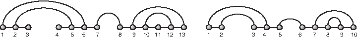
LHS: a diagram over [13] with set of A-arcs {(1, 6), (2, 5), (7, 8), (9, 13), (10, 12)} and set of B-arcs that partition into three backbones: {(1, 2), (2, 3)}, {(4, 5), (5, 6), (6, 7)}, and {(8, 9), (9, 10), (10, 11), (11, 12), (12, 13)}. Here, 3 and 7 are the cut and 3, 4, 11 are isolated vertices. RHS: a matching derived by removing the isolated vertices of the left diagram and relabeling the vertices.

We shall refer to an A-arc simply as an “arc.” Given an arc (i, j), the length of (i, j) is defined by j − i. In particular, when j = i + 1, we refer the arc as a 1-arc. We distinguish exterior and interior arcs, where the former connect a pair of vertices from different backbones and the latter are within a specific one. Diagrams over multiple backbones without exterior arcs are simply disjoint unions of diagrams over one backbone.

An interior stack of length τ on \documentclass{aastex}\usepackage{amsbsy}\usepackage{amsfonts}\usepackage{amssymb}\usepackage{bm}\usepackage{mathrsfs}\usepackage{pifont}\usepackage{stmaryrd}\usepackage{textcomp}\usepackage{portland, xspace}\usepackage{amsmath, amsxtra}\pagestyle{empty}\DeclareMathSizes{10}{9}{7}{6}\begin{document}$$[ i , j ] = \{i , i + 1, \ldots , j - 1, j \} $$\end{document} denoted by \documentclass{aastex}\usepackage{amsbsy}\usepackage{amsfonts}\usepackage{amssymb}\usepackage{bm}\usepackage{mathrsfs}\usepackage{pifont}\usepackage{stmaryrd}\usepackage{textcomp}\usepackage{portland, xspace}\usepackage{amsmath, amsxtra}\pagestyle{empty}\DeclareMathSizes{10}{9}{7}{6}\begin{document}$$SI_{i , j}^{\tau}$$\end{document} is a maximal set (with respect to set inclusion) of exactly τ “parallel” interior arcs, namely \documentclass{aastex}\usepackage{amsbsy}\usepackage{amsfonts}\usepackage{amssymb}\usepackage{bm}\usepackage{mathrsfs}\usepackage{pifont}\usepackage{stmaryrd}\usepackage{textcomp}\usepackage{portland, xspace}\usepackage{amsmath, amsxtra}\pagestyle{empty}\DeclareMathSizes{10}{9}{7}{6}\begin{document}\begin{align*}( ( i , j ) , ( i + 1 , j - 1 ) , \ldots , ( i + ( \tau - 1 ) , j - ( \tau - 1 ) ) ).\end{align*}\end{document}

Furthermore, an interior stack s is τ-canonical if s is of length at least τ. Exterior stacks on [i, j] (SE_i,j) and τ-canonical exterior stacks, \documentclass{aastex}\usepackage{amsbsy}\usepackage{amsfonts}\usepackage{amssymb}\usepackage{bm}\usepackage{mathrsfs}\usepackage{pifont}\usepackage{stmaryrd}\usepackage{textcomp}\usepackage{portland, xspace}\usepackage{amsmath, amsxtra}\pagestyle{empty}\DeclareMathSizes{10}{9}{7}{6}\begin{document}$$SE_{i , j}^{\tau}$$\end{document} , can be similarly defined. We often simply write stack, \documentclass{aastex}\usepackage{amsbsy}\usepackage{amsfonts}\usepackage{amssymb}\usepackage{bm}\usepackage{mathrsfs}\usepackage{pifont}\usepackage{stmaryrd}\usepackage{textcomp}\usepackage{portland, xspace}\usepackage{amsmath, amsxtra}\pagestyle{empty}\DeclareMathSizes{10}{9}{7}{6}\begin{document}$$ST_{i , j}^k$$\end{document} , on [i, j] of length k if its particular type is immaterial. A stack \documentclass{aastex}\usepackage{amsbsy}\usepackage{amsfonts}\usepackage{amssymb}\usepackage{bm}\usepackage{mathrsfs}\usepackage{pifont}\usepackage{stmaryrd}\usepackage{textcomp}\usepackage{portland, xspace}\usepackage{amsmath, amsxtra}\pagestyle{empty}\DeclareMathSizes{10}{9}{7}{6}\begin{document}$$ST_{i , j}^k$$\end{document} on [i, j] of length k naturally induces (k − 1) pairs of intervals of the form \documentclass{aastex}\usepackage{amsbsy}\usepackage{amsfonts}\usepackage{amssymb}\usepackage{bm}\usepackage{mathrsfs}\usepackage{pifont}\usepackage{stmaryrd}\usepackage{textcomp}\usepackage{portland, xspace}\usepackage{amsmath, amsxtra}\pagestyle{empty}\DeclareMathSizes{10}{9}{7}{6}\begin{document}\begin{align*}( [ i + \ell , i + \ell + 1 ] , [\, j - \ell - 1 , j - \ell ] ) \quad {\rm where} \quad 0 \leq \ell \leq k - 2.\end{align*}\end{document}

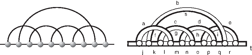
Any of these 2(k − 1) intervals is referred to as a P-interval. Note that P-intervals do only emerge in stacks. If P-intervals emerge, they are always of the form [i, i + 1]. Any interval of the form [i, i + 1] other than a gap or P-interval is called a σ interval. Clearly, a diagram over [n] contains (n − 1) intervals of the form [i, i + 1], and we distinguish the three types: gap intervals, P-intervals, and σ-intervals (Fig. 4). Note that by construction, the sets of gap intervals, P-intervals, and σ-intervals are disjoint.

FIG. 4.

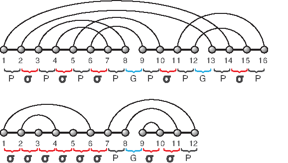
Stacks and intervals: gap intervals, σ-intervals, and P-intervals labeled by G, σ, and P. (Top) There are in total four stacks in the diagram: \documentclass{aastex}\usepackage{amsbsy}\usepackage{amsfonts}\usepackage{amssymb}\usepackage{bm}\usepackage{mathrsfs}\usepackage{pifont}\usepackage{stmaryrd}\usepackage{textcomp}\usepackage{portland, xspace}\usepackage{amsmath, amsxtra}\pagestyle{empty}\DeclareMathSizes{10}{9}{7}{6}\begin{document}$$SE_{1 , 14}^2$$\end{document} , \documentclass{aastex}\usepackage{amsbsy}\usepackage{amsfonts}\usepackage{amssymb}\usepackage{bm}\usepackage{mathrsfs}\usepackage{pifont}\usepackage{stmaryrd}\usepackage{textcomp}\usepackage{portland, xspace}\usepackage{amsmath, amsxtra}\pagestyle{empty}\DeclareMathSizes{10}{9}{7}{6}\begin{document}$$SI_{3 , 8}^2$$\end{document} , \documentclass{aastex}\usepackage{amsbsy}\usepackage{amsfonts}\usepackage{amssymb}\usepackage{bm}\usepackage{mathrsfs}\usepackage{pifont}\usepackage{stmaryrd}\usepackage{textcomp}\usepackage{portland, xspace}\usepackage{amsmath, amsxtra}\pagestyle{empty}\DeclareMathSizes{10}{9}{7}{6}\begin{document}$$SE_{5 , 10}^2$$\end{document} , and \documentclass{aastex}\usepackage{amsbsy}\usepackage{amsfonts}\usepackage{amssymb}\usepackage{bm}\usepackage{mathrsfs}\usepackage{pifont}\usepackage{stmaryrd}\usepackage{textcomp}\usepackage{portland, xspace}\usepackage{amsmath, amsxtra}\pagestyle{empty}\DeclareMathSizes{10}{9}{7}{6}\begin{document}$$SE_{11 , 16}^2$$\end{document} . (Bottom) There are in total four stacks in the diagram: \documentclass{aastex}\usepackage{amsbsy}\usepackage{amsfonts}\usepackage{amssymb}\usepackage{bm}\usepackage{mathrsfs}\usepackage{pifont}\usepackage{stmaryrd}\usepackage{textcomp}\usepackage{portland, xspace}\usepackage{amsmath, amsxtra}\pagestyle{empty}\DeclareMathSizes{10}{9}{7}{6}\begin{document}$$SI_{1 , 6}^1$$\end{document} , \documentclass{aastex}\usepackage{amsbsy}\usepackage{amsfonts}\usepackage{amssymb}\usepackage{bm}\usepackage{mathrsfs}\usepackage{pifont}\usepackage{stmaryrd}\usepackage{textcomp}\usepackage{portland, xspace}\usepackage{amsmath, amsxtra}\pagestyle{empty}\DeclareMathSizes{10}{9}{7}{6}\begin{document}$$SI_{2 , 4}^1$$\end{document} , \documentclass{aastex}\usepackage{amsbsy}\usepackage{amsfonts}\usepackage{amssymb}\usepackage{bm}\usepackage{mathrsfs}\usepackage{pifont}\usepackage{stmaryrd}\usepackage{textcomp}\usepackage{portland, xspace}\usepackage{amsmath, amsxtra}\pagestyle{empty}\DeclareMathSizes{10}{9}{7}{6}\begin{document}$$SE_{7 , 12}^2$$\end{document} , and \documentclass{aastex}\usepackage{amsbsy}\usepackage{amsfonts}\usepackage{amssymb}\usepackage{bm}\usepackage{mathrsfs}\usepackage{pifont}\usepackage{stmaryrd}\usepackage{textcomp}\usepackage{portland, xspace}\usepackage{amsmath, amsxtra}\pagestyle{empty}\DeclareMathSizes{10}{9}{7}{6}\begin{document}$$SI_{9 , 10}^1$$\end{document} . In particular, only \documentclass{aastex}\usepackage{amsbsy}\usepackage{amsfonts}\usepackage{amssymb}\usepackage{bm}\usepackage{mathrsfs}\usepackage{pifont}\usepackage{stmaryrd}\usepackage{textcomp}\usepackage{portland, xspace}\usepackage{amsmath, amsxtra}\pagestyle{empty}\DeclareMathSizes{10}{9}{7}{6}\begin{document}$$SE_{7 , 12}^2$$\end{document} is both 1-canonical and 2-canonical. The other stacks are only 1-canonical but not 2-canonical.

Let ≺ be the partial order on arcs given by (i,j) ≺ (i′, j′) if i′ ≤ i and j ≤ j′. Any diagram has a unique set of maximal arcs (with respect to the partial order), (Fig. 5).

FIG. 5.

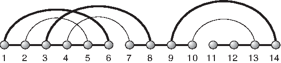
Maximal arcs: the maximal arcs (1, 6), (3, 8), and (9, 14) of a diagram of [14] (bold).

The vertices and arcs of a diagram correspond to nucleotides and base pairs, respectively. For a diagram over b backbones, the leftmost vertex of each backbone denotes the 5′ end of the RNA sequence, while the rightmost vertex denotes the 3′ end. The particular case of b = 2 is referred to as RNA interaction structures (Huang et al., 2009, 2010).

Diagrams over one and two backbones are related by •-product: given two diagrams over two backbones, E₁ and E₂, we can insert E₂ into the gap of E₁ by concatenating the backbones R₂ and R₁ and S₁ and S₂ preserving orientation and relabeling (Fig. 6). This composition is again a diagram over two backbones denoted by E₁ • E₂. It is straightforward to see that • is an associative product with units given by the diagram over two empty backbones. The product • is not commutative.

FIG. 6.

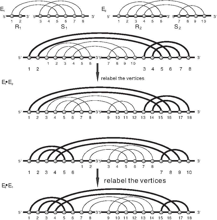
Mapping a diagram over two backbones into a diagram over one backbone by the product •.

2.2. From diagrams to topological surfaces

One approach for deriving meaningful filtration of RNA structure is to pass from diagrams to topological surfaces (Massey, 1967). It is natural to make this transition from combinatorics to topology via fatgraphs (Penner et al., 2010; Penner, 2011). A fatgraph \documentclass{aastex}\usepackage{amsbsy}\usepackage{amsfonts}\usepackage{amssymb}\usepackage{bm}\usepackage{mathrsfs}\usepackage{pifont}\usepackage{stmaryrd}\usepackage{textcomp}\usepackage{portland, xspace}\usepackage{amsmath, amsxtra}\pagestyle{empty}\DeclareMathSizes{10}{9}{7}{6}\begin{document}$${\mathbb G}$$\end{document} , sometimes also called “ribbon graph” or “map,” is a graph G together with a collection of cyclic orderings, called a fattening, one such ordering on the half-edges incident on each vertex. Each fatgraph \documentclass{aastex}\usepackage{amsbsy}\usepackage{amsfonts}\usepackage{amssymb}\usepackage{bm}\usepackage{mathrsfs}\usepackage{pifont}\usepackage{stmaryrd}\usepackage{textcomp}\usepackage{portland, xspace}\usepackage{amsmath, amsxtra}\pagestyle{empty}\DeclareMathSizes{10}{9}{7}{6}\begin{document}$${\mathbb G}$$\end{document} determines an oriented surface F( \documentclass{aastex}\usepackage{amsbsy}\usepackage{amsfonts}\usepackage{amssymb}\usepackage{bm}\usepackage{mathrsfs}\usepackage{pifont}\usepackage{stmaryrd}\usepackage{textcomp}\usepackage{portland, xspace}\usepackage{amsmath, amsxtra}\pagestyle{empty}\DeclareMathSizes{10}{9}{7}{6}\begin{document}$${\mathbb G}$$\end{document} ) as follows: let V (G) be the set of G-vertices and E(G) be the set of G-edges. For each \documentclass{aastex}\usepackage{amsbsy}\usepackage{amsfonts}\usepackage{amssymb}\usepackage{bm}\usepackage{mathrsfs}\usepackage{pifont}\usepackage{stmaryrd}\usepackage{textcomp}\usepackage{portland, xspace}\usepackage{amsmath, amsxtra}\pagestyle{empty}\DeclareMathSizes{10}{9}{7}{6}\begin{document}$$v \in V ( G )$$\end{document} , consider an oriented surface isomorphic to a polygon P_v with 2k sides containing v in its interior where k is the valence of v. The incident edges of v are also incident to a univalent vertex contained in alternating sides of P_v, which are identified with the incident half-edges in the natural way so that the induced counter-clockwise cyclic ordering on the boundary of P_v agrees with the fattening of \documentclass{aastex}\usepackage{amsbsy}\usepackage{amsfonts}\usepackage{amssymb}\usepackage{bm}\usepackage{mathrsfs}\usepackage{pifont}\usepackage{stmaryrd}\usepackage{textcomp}\usepackage{portland, xspace}\usepackage{amsmath, amsxtra}\pagestyle{empty}\DeclareMathSizes{10}{9}{7}{6}\begin{document}$${\mathbb G}$$\end{document} about v (Fig. 7). The surface F( \documentclass{aastex}\usepackage{amsbsy}\usepackage{amsfonts}\usepackage{amssymb}\usepackage{bm}\usepackage{mathrsfs}\usepackage{pifont}\usepackage{stmaryrd}\usepackage{textcomp}\usepackage{portland, xspace}\usepackage{amsmath, amsxtra}\pagestyle{empty}\DeclareMathSizes{10}{9}{7}{6}\begin{document}$${\mathbb G}$$\end{document} ) is the quotient of the disjoint union \documentclass{aastex}\usepackage{amsbsy}\usepackage{amsfonts}\usepackage{amssymb}\usepackage{bm}\usepackage{mathrsfs}\usepackage{pifont}\usepackage{stmaryrd}\usepackage{textcomp}\usepackage{portland, xspace}\usepackage{amsmath, amsxtra}\pagestyle{empty}\DeclareMathSizes{10}{9}{7}{6}\begin{document}$$\sqcup_{v \in V ( G )}P_v$$\end{document} , where the frontier edges, which are oriented with the polygons on their left, are identified by an orientation-reversing homeomorphism if the corresponding half-edges lie in a common edge of G (Fig. 8). This defines the oriented surface F( \documentclass{aastex}\usepackage{amsbsy}\usepackage{amsfonts}\usepackage{amssymb}\usepackage{bm}\usepackage{mathrsfs}\usepackage{pifont}\usepackage{stmaryrd}\usepackage{textcomp}\usepackage{portland, xspace}\usepackage{amsmath, amsxtra}\pagestyle{empty}\DeclareMathSizes{10}{9}{7}{6}\begin{document}$${\mathbb G}$$\end{document} ), which is connected if G is, and is uniquely determined in this case by its genus g = g(G) ≥ 0 and number r = r(G) ≥ 1 of boundary components. Since F( \documentclass{aastex}\usepackage{amsbsy}\usepackage{amsfonts}\usepackage{amssymb}\usepackage{bm}\usepackage{mathrsfs}\usepackage{pifont}\usepackage{stmaryrd}\usepackage{textcomp}\usepackage{portland, xspace}\usepackage{amsmath, amsxtra}\pagestyle{empty}\DeclareMathSizes{10}{9}{7}{6}\begin{document}$${\mathbb G}$$\end{document} ) contains G as a deformation retract, they share the Euler characteristic |V (G)|−|E(G)|, and the genus of F( \documentclass{aastex}\usepackage{amsbsy}\usepackage{amsfonts}\usepackage{amssymb}\usepackage{bm}\usepackage{mathrsfs}\usepackage{pifont}\usepackage{stmaryrd}\usepackage{textcomp}\usepackage{portland, xspace}\usepackage{amsmath, amsxtra}\pagestyle{empty}\DeclareMathSizes{10}{9}{7}{6}\begin{document}$${\mathbb G}$$\end{document} ) is for diagrams over one backbone 2 − 2g − r = |V (G)| − |E(G)| = 1 − n and for diagrams over two backbones given by \documentclass{aastex}\usepackage{amsbsy}\usepackage{amsfonts}\usepackage{amssymb}\usepackage{bm}\usepackage{mathrsfs}\usepackage{pifont}\usepackage{stmaryrd}\usepackage{textcomp}\usepackage{portland, xspace}\usepackage{amsmath, amsxtra}\pagestyle{empty}\DeclareMathSizes{10}{9}{7}{6}\begin{document}\begin{align*}2 - 2g - r = \mid V ( G ) \mid - \mid E ( G ) \mid = 2 - n , \tag{2.1}\end{align*}\end{document}

FIG. 7.

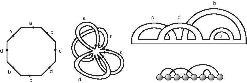
Computing the number of boundary components. The diagram contains 5+9 edges and 10 vertices. We follow the alternating paths described in the text and observe that there are exactly two boundary components (bold and thin). The genus of the diagram is given by \documentclass{aastex}\usepackage{amsbsy}\usepackage{amsfonts}\usepackage{amssymb}\usepackage{bm}\usepackage{mathrsfs}\usepackage{pifont}\usepackage{stmaryrd}\usepackage{textcomp}\usepackage{portland, xspace}\usepackage{amsmath, amsxtra}\pagestyle{empty}\DeclareMathSizes{10}{9}{7}{6}\begin{document}$$1 - \frac {1} {2} ( 10 - 14 + 2 ) = 2$$\end{document} .

FIG. 8.

Case study for a diagram over one backbone: equivalence between a pairwise identification of the sides of an octagon (left), the surface F( \documentclass{aastex}\usepackage{amsbsy}\usepackage{amsfonts}\usepackage{amssymb}\usepackage{bm}\usepackage{mathrsfs}\usepackage{pifont}\usepackage{stmaryrd}\usepackage{textcomp}\usepackage{portland, xspace}\usepackage{amsmath, amsxtra}\pagestyle{empty}\DeclareMathSizes{10}{9}{7}{6}\begin{document}$${\mathbb G}$$\end{document} ) where all vertices of the backbone are collapsed into a single vertex (note we therefore have 2 − 2g − r = 1 − n) (middle) and the surface F( \documentclass{aastex}\usepackage{amsbsy}\usepackage{amsfonts}\usepackage{amssymb}\usepackage{bm}\usepackage{mathrsfs}\usepackage{pifont}\usepackage{stmaryrd}\usepackage{textcomp}\usepackage{portland, xspace}\usepackage{amsmath, amsxtra}\pagestyle{empty}\DeclareMathSizes{10}{9}{7}{6}\begin{document}$${\mathbb G}$$\end{document} ) induced by a linear chord diagram G (right).

where n denotes the number of arcs.

For an RNA diagram, we may draw a representation as usual so that the backbone is a horizontal line oriented from left to right, and the arcs lie in the upper half-plane. This determines a unique fattening on any diagram (cf. the leftmost two panels in Fig. 9 for the fatgraph and its corresponding surface). Each boundary component of F( \documentclass{aastex}\usepackage{amsbsy}\usepackage{amsfonts}\usepackage{amssymb}\usepackage{bm}\usepackage{mathrsfs}\usepackage{pifont}\usepackage{stmaryrd}\usepackage{textcomp}\usepackage{portland, xspace}\usepackage{amsmath, amsxtra}\pagestyle{empty}\DeclareMathSizes{10}{9}{7}{6}\begin{document}$${\mathbb G}$$\end{document} ) determines a closed edge-path or cycle on G, oriented with the surface lying on its left. In particular, a neighborhood of each edge inherits an orientation from that of F( \documentclass{aastex}\usepackage{amsbsy}\usepackage{amsfonts}\usepackage{amssymb}\usepackage{bm}\usepackage{mathrsfs}\usepackage{pifont}\usepackage{stmaryrd}\usepackage{textcomp}\usepackage{portland, xspace}\usepackage{amsmath, amsxtra}\pagestyle{empty}\DeclareMathSizes{10}{9}{7}{6}\begin{document}$${\mathbb G}$$\end{document} ), which combines to give the oriented cycles as depicted in the third panel of Figure 9. Without affecting topological type of the constructed surface, one may collapse each backbone to a single vertex with the induced fattening called the polygonal model of the RNA, as illustrated in the rightmost panels of Figure 9. It is the orientation of each backbone from the 5′ end to the 3′ end that allows us to transform the fatgraph of an RNA-structure or RNA-interaction into a fatgraph with one or two vertices.

FIG. 9.

(A) The fatgraph of a diagram and its reduction to a single vertex. Contracting the backbone of a diagram into a single vertex decreases the length of the boundary components and preserves the genus. (B) Inflation of edges and vertices to ribbons and discs, as well as walking along the boundary components. Here we have six vertices, seven edges, and one boundary component. The corresponding surface has Euler characteristic χ = −1 and genus one. At the last step, we collapse each backbone into a single disc again preserving genus. The backbone of the polymer can be recovered by inflating each disk to a backbone segment.

This backbone collapse preserves orientation, Euler characteristic, and genus by construction. It is reversible by inflating each vertex to form a backbone. Using the collapsed fatgraph representation, we see that for a connected diagram over [n] with b backbones, the genus g of the surface (with boundary) is determined by the number n of arcs as well as the number r of boundary components, namely, 2 − 2g− r = |V (G)| − |E(G)| = b − n (cf. Fig. 9), in which v and e are the cardinalities of the vertex set and edge set in the diagram, respectively.

2.3. Shadows

A shadow is a diagram with no noncrossing arcs or isolated vertices in which each stack has length one. The shadow of a diagram is obtained by removing all noncrossing arcs, deleting all isolated vertices, and collapsing each induced stack to a single arc (cf. Fig. 10). Note that projecting into the shadow does not affect genus. In case there are no crossing arcs in a diagram X, then the shadow of X becomes an empty diagram on the same number of backbones as X as in Figure 10C. By definition, any empty backbone contributes one boundary component. For example, for a diagram X over b backbones that contains no crossing arcs, the shadow of X is a sequence of b empty backbones with b boundary components.

FIG. 10.

Shadows: (A) a diagram over one backbone and its shadow, (B) a diagram over two backbones whose shadow is again a diagram over two backbones, and (C) a diagram whose shadow is an empty backbone.

Theorem 1

(Andersen et al., 2012) A shadow over two backbones has the following properties:

(a) A shadow of genus g ≥ 1 over two backbones contains at least (2g + 1) and at most 6(g + 1) − 2 arcs; a shadow of genus 0 has at least 2 and at most 4 arcs. in particular, the set of such shadows is finite;

(b) For any (2g + 1) ≤ ℓ ≤ 6(g + 1) − 2 in case of g ≥ 1 and 2 ≤ ℓ ≤ 4 in case of g = 0, there exists some shadow over two backbones with genus g containing exactly ℓ arcs.

Proof. See Appendix A-1. ■

2.4. Irreducibility

A diagram E over b backbones is called irreducible if it is connected and for any two arcs, α₁,α_k contained in E, there exists a sequence of arcs \documentclass{aastex}\usepackage{amsbsy}\usepackage{amsfonts}\usepackage{amssymb}\usepackage{bm}\usepackage{mathrsfs}\usepackage{pifont}\usepackage{stmaryrd}\usepackage{textcomp}\usepackage{portland, xspace}\usepackage{amsmath, amsxtra}\pagestyle{empty}\DeclareMathSizes{10}{9}{7}{6}\begin{document}\begin{align*}( \alpha_1 , \alpha_2 , \ldots , \alpha_{k - 1} , \alpha_k )\end{align*}\end{document}

such that (α_i, α_i₊₁) are crossing. An irreducible shadow is simply a diagram that is a shadow as well as an irreducible diagram. As proved in Andersen et al. (2012), there is the following corollary of Theorem 1.

Corollary 1

An irreducible shadow having genus g = 0 over two backbones contains at least 2 and at most 4 arcs, and for 2 ≤ ℓ ≤ 4, there exists an irreducible shadow of genus g = 0 over two backbones having exactly ℓ arcs. An irreducible shadow having genus g≥1 has the following properties:

(a) every irreducible shadow with genus g over two backbones contains at least 2g + 1 and at most 6(g + 1) − 2 arcs;

(b) for arbitrary genus g and any 2g + 1 ≤ ℓ ≤ 6g − 2, there exists an irreducible shadow of genus g over one backbone having exactly ℓ arcs.

Proof. See Appendix A-2. ■

Let X be a diagram. We call S′ an irreducible shadow of X (irreducible X-shadow) if S′ is an irreducible shadow and any arc in S′ is contained in X. S′ is a (g, b, m)-shadow if S′ is a diagram over b backbones having genus g and m arcs. The set of irreducible (g, b, m)-shadows is denoted by \documentclass{aastex}\usepackage{amsbsy}\usepackage{amsfonts}\usepackage{amssymb}\usepackage{bm}\usepackage{mathrsfs}\usepackage{pifont}\usepackage{stmaryrd}\usepackage{textcomp}\usepackage{portland, xspace}\usepackage{amsmath, amsxtra}\pagestyle{empty}\DeclareMathSizes{10}{9}{7}{6}\begin{document}$$ {\cal J}_{g , b , m}$$\end{document} . Let \documentclass{aastex}\usepackage{amsbsy}\usepackage{amsfonts}\usepackage{amssymb}\usepackage{bm}\usepackage{mathrsfs}\usepackage{pifont}\usepackage{stmaryrd}\usepackage{textcomp}\usepackage{portland, xspace}\usepackage{amsmath, amsxtra}\pagestyle{empty}\DeclareMathSizes{10}{9}{7}{6}\begin{document}$${\cal J}_{g , b} = \cup_{m} {\cal J}_{g , b , m}$$\end{document} .

According to Theorem 1, the generating function \documentclass{aastex}\usepackage{amsbsy}\usepackage{amsfonts}\usepackage{amssymb}\usepackage{bm}\usepackage{mathrsfs}\usepackage{pifont}\usepackage{stmaryrd}\usepackage{textcomp}\usepackage{portland, xspace}\usepackage{amsmath, amsxtra}\pagestyle{empty}\DeclareMathSizes{10}{9}{7}{6}\begin{document}$$\textbf{I}_{g , b} ( u ) = \sum \ \textbf{i}_{g , b} ( m ) u^m$$\end{document} of the combinatorial class \documentclass{aastex}\usepackage{amsbsy}\usepackage{amsfonts}\usepackage{amssymb}\usepackage{bm}\usepackage{mathrsfs}\usepackage{pifont}\usepackage{stmaryrd}\usepackage{textcomp}\usepackage{portland, xspace}\usepackage{amsmath, amsxtra}\pagestyle{empty}\DeclareMathSizes{10}{9}{7}{6}\begin{document}$${\cal J}_{g , b}$$\end{document} is a polynomial. Indeed this can be shown in two ways: first, since m is bounded (Theorem 1), we may simply exhaustively enumerate all such irreducible shadows, second, we can use the genus filtration of γ structures in order to establish a recursion of \documentclass{aastex}\usepackage{amsbsy}\usepackage{amsfonts}\usepackage{amssymb}\usepackage{bm}\usepackage{mathrsfs}\usepackage{pifont}\usepackage{stmaryrd}\usepackage{textcomp}\usepackage{portland, xspace}\usepackage{amsmath, amsxtra}\pagestyle{empty}\DeclareMathSizes{10}{9}{7}{6}\begin{document}$${\cal J}_{g , b}$$\end{document} . Accordingly, we obtain the generating polynomials for I_g,b(u) for 0 ≤ g ≤ 1 and 1 ≤ b ≤ 2 as follows. \documentclass{aastex}\usepackage{amsbsy}\usepackage{amsfonts}\usepackage{amssymb}\usepackage{bm}\usepackage{mathrsfs}\usepackage{pifont}\usepackage{stmaryrd}\usepackage{textcomp}\usepackage{portland, xspace}\usepackage{amsmath, amsxtra}\pagestyle{empty}\DeclareMathSizes{10}{9}{7}{6}\begin{document}\begin{align*} & \textbf{I}_{1 , 1} ( z ) = z^2 + 2z^3 + z^4 , \\ & \textbf{I}_{2 , 1} ( z ) = 17z^4 + 160z^5 + 566z^6 + 1004z^7 + 961z^8 + 476z^9 + 96z^{10} , \\ & \textbf{I}_{0 , 2} ( u ) = 3u^2 + 3u^3 + u^4 , \\ & \textbf{I}_{1 , 2} ( u ) = 11u^3 + 137u^4 + 656u^5 + 1520u^6 + 1951u^7 + 1436u^8 + 572u^9 + 96u^{10}.\end{align*}\end{document}

We display the seven irreducible shadows over two backbones of genus 0 in Figure 11.

FIG. 11.

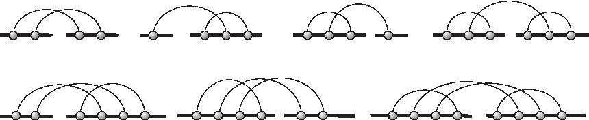
There are exactly seven (3+3+1) irreducible shadows over two backbones of genus 0, in which there are 3/3/1 irreducible shadows with 2/3/4 arcs that correspond to the monomials 3u², 3u³, and u⁴ of I_0,2(u).

2.5. γ-Structures

A diagram is a γ-structure if it is connected and all its irreducible shadows have genus at most γ. A γ-matching is a γ-structure as well as a matching. The combinatorial class of γ-matchings over one backbone is denoted by \documentclass{aastex}\usepackage{amsbsy}\usepackage{amsfonts}\usepackage{amssymb}\usepackage{bm}\usepackage{mathrsfs}\usepackage{pifont}\usepackage{stmaryrd}\usepackage{textcomp}\usepackage{portland, xspace}\usepackage{amsmath, amsxtra}\pagestyle{empty}\DeclareMathSizes{10}{9}{7}{6}\begin{document}$${\cal H}_{\gamma}$$\end{document} , for which the corresponding generating function H_γ(u) has been derived in Han and Reidys (2012) as follows:

Theorem 2

Let \documentclass{aastex}\usepackage{amsbsy}\usepackage{amsfonts}\usepackage{amssymb}\usepackage{bm}\usepackage{mathrsfs}\usepackage{pifont}\usepackage{stmaryrd}\usepackage{textcomp}\usepackage{portland, xspace}\usepackage{amsmath, amsxtra}\pagestyle{empty}\DeclareMathSizes{10}{9}{7}{6}\begin{document}$$R = {\mathbb Z} [ u ]$$\end{document} . Then H_γ(u) satisfies \documentclass{aastex}\usepackage{amsbsy}\usepackage{amsfonts}\usepackage{amssymb}\usepackage{bm}\usepackage{mathrsfs}\usepackage{pifont}\usepackage{stmaryrd}\usepackage{textcomp}\usepackage{portland, xspace}\usepackage{amsmath, amsxtra}\pagestyle{empty}\DeclareMathSizes{10}{9}{7}{6}\begin{document}\begin{align*} \textbf{H} _ {\gamma} ( u ) ^ {- 1} = 1 - \left( u \ \textbf{H} _ {\gamma} ( u ) + \textbf{H} _ {\gamma} ^ {- 1} ( u ) \sum_ {g \le \gamma} \textbf{I} _ {g , 1} \left( \frac {u \ \textbf{H} _ {\gamma} ^ {2} ( u )} {1 - u \ \textbf{H} _ {\gamma} ^ {2} ( u )} \right) \right). \tag {2.2} \end{align*}\end{document}

Furthermore, Equation (2.2) determines H_γ(u) uniquely. In case of γ = 1, the coefficients of H₁(u) are asymptotically given by \documentclass{aastex}\usepackage{amsbsy}\usepackage{amsfonts}\usepackage{amssymb}\usepackage{bm}\usepackage{mathrsfs}\usepackage{pifont}\usepackage{stmaryrd}\usepackage{textcomp}\usepackage{portland, xspace}\usepackage{amsmath, amsxtra}\pagestyle{empty}\DeclareMathSizes{10}{9}{7}{6}\begin{document}\begin{align*}[ z^n ] \textbf{H}_{1} ( u ) \,\sim\, k n^{- 3 / 2} \ \left( \rho^{- 1} \right) ^n \tag{2.3}\end{align*}\end{document}

in which k is some positive constant and ρ⁻¹≈8.28425.

The combinatorial classes of γ-matchings over two backbones is denoted by \documentclass{aastex}\usepackage{amsbsy}\usepackage{amsfonts}\usepackage{amssymb}\usepackage{bm}\usepackage{mathrsfs}\usepackage{pifont}\usepackage{stmaryrd}\usepackage{textcomp}\usepackage{portland, xspace}\usepackage{amsmath, amsxtra}\pagestyle{empty}\DeclareMathSizes{10}{9}{7}{6}\begin{document}$${\cal Q}_{\gamma}$$\end{document} . We also call the γ-structure over two backbones γ-interaction structures. In this article, we focus on deriving the combinatorial properties of these γ-interaction structures.

2.6. Symbolic notations

In the following, given a particular set of diagrams \documentclass{aastex}\usepackage{amsbsy}\usepackage{amsfonts}\usepackage{amssymb}\usepackage{bm}\usepackage{mathrsfs}\usepackage{pifont}\usepackage{stmaryrd}\usepackage{textcomp}\usepackage{portland, xspace}\usepackage{amsmath, amsxtra}\pagestyle{empty}\DeclareMathSizes{10}{9}{7}{6}\begin{document}$${\cal K}$$\end{document} , we denote its corresponding generating function by K(u) = ∑_n k(n)uⁿ, where k(n) denotes the number of diagrams in \documentclass{aastex}\usepackage{amsbsy}\usepackage{amsfonts}\usepackage{amssymb}\usepackage{bm}\usepackage{mathrsfs}\usepackage{pifont}\usepackage{stmaryrd}\usepackage{textcomp}\usepackage{portland, xspace}\usepackage{amsmath, amsxtra}\pagestyle{empty}\DeclareMathSizes{10}{9}{7}{6}\begin{document}$${\cal K}$$\end{document} that contain exactly n arcs. We systematically use caligraphic, bold capital, and bold roman fonts in order to denote combinatorial classes, generating functions and their coefficients, respectively. We shall frequently encounter the following three combinatorial classes: \documentclass{aastex}\usepackage{amsbsy}\usepackage{amsfonts}\usepackage{amssymb}\usepackage{bm}\usepackage{mathrsfs}\usepackage{pifont}\usepackage{stmaryrd}\usepackage{textcomp}\usepackage{portland, xspace}\usepackage{amsmath, amsxtra}\pagestyle{empty}\DeclareMathSizes{10}{9}{7}{6}\begin{document}$${\cal E}$$\end{document} (neutral class that includes only one element of size 0), \documentclass{aastex}\usepackage{amsbsy}\usepackage{amsfonts}\usepackage{amssymb}\usepackage{bm}\usepackage{mathrsfs}\usepackage{pifont}\usepackage{stmaryrd}\usepackage{textcomp}\usepackage{portland, xspace}\usepackage{amsmath, amsxtra}\pagestyle{empty}\DeclareMathSizes{10}{9}{7}{6}\begin{document}$${\cal Z}$$\end{document} (vertices), and \documentclass{aastex}\usepackage{amsbsy}\usepackage{amsfonts}\usepackage{amssymb}\usepackage{bm}\usepackage{mathrsfs}\usepackage{pifont}\usepackage{stmaryrd}\usepackage{textcomp}\usepackage{portland, xspace}\usepackage{amsmath, amsxtra}\pagestyle{empty}\DeclareMathSizes{10}{9}{7}{6}\begin{document}$${\cal U}$$\end{document} (arcs).

3. γ-Matchings Over Two Backbones

In this section, we compute the generating function Q_γ(u) of γ-matchings over two backbones in Theorem 3 and derive asymptotic formulas of Q_γ(u) for the cases of γ = 0, 1. For this purpose, we need to introduce the following particular structures that will serve as building blocks in calculating Q_γ(u).

Let \documentclass{aastex}\usepackage{amsbsy}\usepackage{amsfonts}\usepackage{amssymb}\usepackage{bm}\usepackage{mathrsfs}\usepackage{pifont}\usepackage{stmaryrd}\usepackage{textcomp}\usepackage{portland, xspace}\usepackage{amsmath, amsxtra}\pagestyle{empty}\DeclareMathSizes{10}{9}{7}{6}\begin{document}$${\cal A}_{\gamma}$$\end{document} denote the set of γ-matchings M over two backbones such that any pair of exterior arcs in M (can be empty) are nesting to each other. A function Level : \documentclass{aastex}\usepackage{amsbsy}\usepackage{amsfonts}\usepackage{amssymb}\usepackage{bm}\usepackage{mathrsfs}\usepackage{pifont}\usepackage{stmaryrd}\usepackage{textcomp}\usepackage{portland, xspace}\usepackage{amsmath, amsxtra}\pagestyle{empty}\DeclareMathSizes{10}{9}{7}{6}\begin{document}$${\cal Q}_{\gamma} \rightarrow {\mathbb N}_0$$\end{document} maps a \documentclass{aastex}\usepackage{amsbsy}\usepackage{amsfonts}\usepackage{amssymb}\usepackage{bm}\usepackage{mathrsfs}\usepackage{pifont}\usepackage{stmaryrd}\usepackage{textcomp}\usepackage{portland, xspace}\usepackage{amsmath, amsxtra}\pagestyle{empty}\DeclareMathSizes{10}{9}{7}{6}\begin{document}$${\cal Q}_{\gamma}$$\end{document} -matching to its (nonnegative) number of exterior stacks. Set \documentclass{aastex}\usepackage{amsbsy}\usepackage{amsfonts}\usepackage{amssymb}\usepackage{bm}\usepackage{mathrsfs}\usepackage{pifont}\usepackage{stmaryrd}\usepackage{textcomp}\usepackage{portland, xspace}\usepackage{amsmath, amsxtra}\pagestyle{empty}\DeclareMathSizes{10}{9}{7}{6}\begin{document}$${\cal A}_{\gamma , \ell}$$\end{document} denote the set of elements \documentclass{aastex}\usepackage{amsbsy}\usepackage{amsfonts}\usepackage{amssymb}\usepackage{bm}\usepackage{mathrsfs}\usepackage{pifont}\usepackage{stmaryrd}\usepackage{textcomp}\usepackage{portland, xspace}\usepackage{amsmath, amsxtra}\pagestyle{empty}\DeclareMathSizes{10}{9}{7}{6}\begin{document}$$M \in {\cal A}_{\gamma}$$\end{document} such that Level(M) = ℓ. Clearly, there exists \documentclass{aastex}\usepackage{amsbsy}\usepackage{amsfonts}\usepackage{amssymb}\usepackage{bm}\usepackage{mathrsfs}\usepackage{pifont}\usepackage{stmaryrd}\usepackage{textcomp}\usepackage{portland, xspace}\usepackage{amsmath, amsxtra}\pagestyle{empty}\DeclareMathSizes{10}{9}{7}{6}\begin{document}$${\cal A}_{\gamma} = \dot{\bigcup}_{\ell \geq 0} {\cal A}_{\gamma , \ell}$$\end{document} .

Lemma 1

Let a_γ(n) denote the number of \documentclass{aastex}\usepackage{amsbsy}\usepackage{amsfonts}\usepackage{amssymb}\usepackage{bm}\usepackage{mathrsfs}\usepackage{pifont}\usepackage{stmaryrd}\usepackage{textcomp}\usepackage{portland, xspace}\usepackage{amsmath, amsxtra}\pagestyle{empty}\DeclareMathSizes{10}{9}{7}{6}\begin{document}$${\cal A}_{\gamma}$$\end{document} -matchings with n arcs. The generating function A_γ(u) = ∑_n a_γ(n)uⁿ is given by \documentclass{aastex}\usepackage{amsbsy}\usepackage{amsfonts}\usepackage{amssymb}\usepackage{bm}\usepackage{mathrsfs}\usepackage{pifont}\usepackage{stmaryrd}\usepackage{textcomp}\usepackage{portland, xspace}\usepackage{amsmath, amsxtra}\pagestyle{empty}\DeclareMathSizes{10}{9}{7}{6}\begin{document}\begin{align} \textbf{A} _ {\gamma} ( u ) = \frac {\textbf{H} ^ {2} _ {\gamma} ( u )} {1 - u \cdot \textbf{H} ^ {2} _ {\gamma} ( u )} . \tag {3.1} \end{align}\end{document}

Proof. Since \documentclass{aastex}\usepackage{amsbsy}\usepackage{amsfonts}\usepackage{amssymb}\usepackage{bm}\usepackage{mathrsfs}\usepackage{pifont}\usepackage{stmaryrd}\usepackage{textcomp}\usepackage{portland, xspace}\usepackage{amsmath, amsxtra}\pagestyle{empty}\DeclareMathSizes{10}{9}{7}{6}\begin{document}$${\cal A}_{\gamma} = \dot{\bigcup}_{\ell \geq 0} {\cal A}_{\gamma , \ell}$$\end{document} , A_γ(u) is derived by recursively calculating \documentclass{aastex}\usepackage{amsbsy}\usepackage{amsfonts}\usepackage{amssymb}\usepackage{bm}\usepackage{mathrsfs}\usepackage{pifont}\usepackage{stmaryrd}\usepackage{textcomp}\usepackage{portland, xspace}\usepackage{amsmath, amsxtra}\pagestyle{empty}\DeclareMathSizes{10}{9}{7}{6}\begin{document}$${\cal A}_{\gamma , \ell}$$\end{document} and summing over all possible ℓ ≥ 0 afterward.

When ℓ = 0, it is obvious that \documentclass{aastex}\usepackage{amsbsy}\usepackage{amsfonts}\usepackage{amssymb}\usepackage{bm}\usepackage{mathrsfs}\usepackage{pifont}\usepackage{stmaryrd}\usepackage{textcomp}\usepackage{portland, xspace}\usepackage{amsmath, amsxtra}\pagestyle{empty}\DeclareMathSizes{10}{9}{7}{6}\begin{document}$${\cal A}_{\gamma , 0} = {\cal H}_{\gamma} \times {\cal H}_{\gamma}$$\end{document} .

In case of ℓ > 0, set s^⋆ to denote the particular \documentclass{aastex}\usepackage{amsbsy}\usepackage{amsfonts}\usepackage{amssymb}\usepackage{bm}\usepackage{mathrsfs}\usepackage{pifont}\usepackage{stmaryrd}\usepackage{textcomp}\usepackage{portland, xspace}\usepackage{amsmath, amsxtra}\pagestyle{empty}\DeclareMathSizes{10}{9}{7}{6}\begin{document}$${\cal A}_{\gamma , \ell}$$\end{document} -matching over [2ℓ] consisting of ℓ noncrossing exterior arcs. Then any \documentclass{aastex}\usepackage{amsbsy}\usepackage{amsfonts}\usepackage{amssymb}\usepackage{bm}\usepackage{mathrsfs}\usepackage{pifont}\usepackage{stmaryrd}\usepackage{textcomp}\usepackage{portland, xspace}\usepackage{amsmath, amsxtra}\pagestyle{empty}\DeclareMathSizes{10}{9}{7}{6}\begin{document}$${\cal A}_{\gamma , \ell}$$\end{document} matching s can be obtained from s^⋆ in three steps (Fig. 12):

FIG. 12.
The construction of \documentclass{aastex}\usepackage{amsbsy}\usepackage{amsfonts}\usepackage{amssymb}\usepackage{bm}\usepackage{mathrsfs}\usepackage{pifont}\usepackage{stmaryrd}\usepackage{textcomp}\usepackage{portland, xspace}\usepackage{amsmath, amsxtra}\pagestyle{empty}\DeclareMathSizes{10}{9}{7}{6}\begin{document}$${\cal A}_{\gamma , \ell}$$\end{document} in the case of ℓ = 3.

(I) Insert nonempty γ-matchings into at least one of the two intervals of each pair of intervals ([i, i + 1], [2ℓ − i, 2ℓ − i + 1]). Since there are ℓ − 1 pairs of such intervals in s^⋆, we obtain the class \documentclass{aastex}\usepackage{amsbsy}\usepackage{amsfonts}\usepackage{amssymb}\usepackage{bm}\usepackage{mathrsfs}\usepackage{pifont}\usepackage{stmaryrd}\usepackage{textcomp}\usepackage{portland, xspace}\usepackage{amsmath, amsxtra}\pagestyle{empty}\DeclareMathSizes{10}{9}{7}{6}\begin{document}$${\cal U}^{\ell} \times ( {\cal H}_{\gamma}^2 - {\cal E} ) ^{\ell - 1}$$\end{document} ;

(II) inflate each exterior arc in the derived matching into an exterior stack. Since there are in total ℓ exterior arcs after Step (I), we derive the class \documentclass{aastex}\usepackage{amsbsy}\usepackage{amsfonts}\usepackage{amssymb}\usepackage{bm}\usepackage{mathrsfs}\usepackage{pifont}\usepackage{stmaryrd}\usepackage{textcomp}\usepackage{portland, xspace}\usepackage{amsmath, amsxtra}\pagestyle{empty}\DeclareMathSizes{10}{9}{7}{6}\begin{document}$${\cal N}_{\gamma , \ell} = ( {\cal U} \times \textbf{SEQ} ( {\cal U} ) ) ^{\ell} \times ( {\cal H}_{\gamma}^2 - {\cal E} ) ^{\ell - 1}$$\end{document} , in which \documentclass{aastex}\usepackage{amsbsy}\usepackage{amsfonts}\usepackage{amssymb}\usepackage{bm}\usepackage{mathrsfs}\usepackage{pifont}\usepackage{stmaryrd}\usepackage{textcomp}\usepackage{portland, xspace}\usepackage{amsmath, amsxtra}\pagestyle{empty}\DeclareMathSizes{10}{9}{7}{6}\begin{document}$$\textbf{SEQ} ( {\cal U} ) = {\cal E} + {\cal U} + {\cal U}^2 + \cdots ;$$\end{document}

(III) concatenate each end of the (two) backbones with a γ-matching (possible empty), \documentclass{aastex}\usepackage{amsbsy}\usepackage{amsfonts}\usepackage{amssymb}\usepackage{bm}\usepackage{mathrsfs}\usepackage{pifont}\usepackage{stmaryrd}\usepackage{textcomp}\usepackage{portland, xspace}\usepackage{amsmath, amsxtra}\pagestyle{empty}\DeclareMathSizes{10}{9}{7}{6}\begin{document}$${\cal H}_{\gamma}^4 \bullet {\cal N}_{\gamma , \ell}$$\end{document} .

Accordingly, we derive \documentclass{aastex}\usepackage{amsbsy}\usepackage{amsfonts}\usepackage{amssymb}\usepackage{bm}\usepackage{mathrsfs}\usepackage{pifont}\usepackage{stmaryrd}\usepackage{textcomp}\usepackage{portland, xspace}\usepackage{amsmath, amsxtra}\pagestyle{empty}\DeclareMathSizes{10}{9}{7}{6}\begin{document}$${\cal A}_{\gamma , \ell} = {\cal H}^{4}_{\gamma} \times ( {\cal U} \times \textbf{SEQ} ( {\cal U} ) ) ^{\ell} \times ( {\cal H}^{2}_{\gamma} - {\cal E} ) ^{\ell - 1}$$\end{document} for any ℓ ≥ 1. Sum over all ℓ ≥ 0 and the lemma follows. ■

Theorem 3

The generating function of γ-matchings over two backbones satisfies \documentclass{aastex}\usepackage{amsbsy}\usepackage{amsfonts}\usepackage{amssymb}\usepackage{bm}\usepackage{mathrsfs}\usepackage{pifont}\usepackage{stmaryrd}\usepackage{textcomp}\usepackage{portland, xspace}\usepackage{amsmath, amsxtra}\pagestyle{empty}\DeclareMathSizes{10}{9}{7}{6}\begin{document}\begin{align} \textbf{Q} _ {\gamma} ( u ) = \frac {\textbf{H} _ {\gamma} ^ {2} ( u ) \cdot \left( u \textbf{H} ^ {2} _ {\gamma} ( u ) + \sum_ {g \leq \gamma} \textbf{I} _ {g , 2} \left( \frac {u \cdot \textbf{H} _ {\gamma} ^ {2} ( u )} {1 - u \textbf{H} ^ {2} _ {\gamma} ( u )} \right) \right)} {1 - u \textbf{H} _ {\gamma} ^ {2} ( u ) - \sum_ {g \leq \gamma} \textbf{I} _ {g , 2} \left( \frac {u \cdot \textbf{H} _ {\gamma} ^ {2} ( u )} {1 - u \textbf{H} ^ {2} _ {\gamma} ( u )} \right)} . \tag {3.2} \end{align}\end{document}

Proof. To calculate Q_γ(u), the key is to consider the set of irreducible shadows that contain at least one exterior arc of an arbitrary \documentclass{aastex}\usepackage{amsbsy}\usepackage{amsfonts}\usepackage{amssymb}\usepackage{bm}\usepackage{mathrsfs}\usepackage{pifont}\usepackage{stmaryrd}\usepackage{textcomp}\usepackage{portland, xspace}\usepackage{amsmath, amsxtra}\pagestyle{empty}\DeclareMathSizes{10}{9}{7}{6}\begin{document}$${\cal Q}_{\gamma}$$\end{document} -matching, say M. Denote this set by \documentclass{aastex}\usepackage{amsbsy}\usepackage{amsfonts}\usepackage{amssymb}\usepackage{bm}\usepackage{mathrsfs}\usepackage{pifont}\usepackage{stmaryrd}\usepackage{textcomp}\usepackage{portland, xspace}\usepackage{amsmath, amsxtra}\pagestyle{empty}\DeclareMathSizes{10}{9}{7}{6}\begin{document}$${\cal S}h ( M )$$\end{document} . We observe that all elements in \documentclass{aastex}\usepackage{amsbsy}\usepackage{amsfonts}\usepackage{amssymb}\usepackage{bm}\usepackage{mathrsfs}\usepackage{pifont}\usepackage{stmaryrd}\usepackage{textcomp}\usepackage{portland, xspace}\usepackage{amsmath, amsxtra}\pagestyle{empty}\DeclareMathSizes{10}{9}{7}{6}\begin{document}$${\cal S}h ( M )$$\end{document} are nested via •-product. In particular, there exists exactly only one element in \documentclass{aastex}\usepackage{amsbsy}\usepackage{amsfonts}\usepackage{amssymb}\usepackage{bm}\usepackage{mathrsfs}\usepackage{pifont}\usepackage{stmaryrd}\usepackage{textcomp}\usepackage{portland, xspace}\usepackage{amsmath, amsxtra}\pagestyle{empty}\DeclareMathSizes{10}{9}{7}{6}\begin{document}$${\cal S}h ( M )$$\end{document} consisting of maximal arcs. This is because, by construction, any concatenation of two matchings (over two backbones) will give rise to a matching over three backbones.

Let \documentclass{aastex}\usepackage{amsbsy}\usepackage{amsfonts}\usepackage{amssymb}\usepackage{bm}\usepackage{mathrsfs}\usepackage{pifont}\usepackage{stmaryrd}\usepackage{textcomp}\usepackage{portland, xspace}\usepackage{amsmath, amsxtra}\pagestyle{empty}\DeclareMathSizes{10}{9}{7}{6}\begin{document}$${\cal Q}_{\gamma , t}$$\end{document} denote the set of Q_γ-matchings s such that \documentclass{aastex}\usepackage{amsbsy}\usepackage{amsfonts}\usepackage{amssymb}\usepackage{bm}\usepackage{mathrsfs}\usepackage{pifont}\usepackage{stmaryrd}\usepackage{textcomp}\usepackage{portland, xspace}\usepackage{amsmath, amsxtra}\pagestyle{empty}\DeclareMathSizes{10}{9}{7}{6}\begin{document}$$\mid {\cal S}h ( s ) \mid = t$$\end{document} . Then there is \documentclass{aastex}\usepackage{amsbsy}\usepackage{amsfonts}\usepackage{amssymb}\usepackage{bm}\usepackage{mathrsfs}\usepackage{pifont}\usepackage{stmaryrd}\usepackage{textcomp}\usepackage{portland, xspace}\usepackage{amsmath, amsxtra}\pagestyle{empty}\DeclareMathSizes{10}{9}{7}{6}\begin{document}$${\cal Q}_{\gamma} = \dot{\bigcup}_{t = 0} {\cal Q}_{\gamma , t}$$\end{document} . Therefore the calculation of Q_γ(u) can be retrieved by calculations of \documentclass{aastex}\usepackage{amsbsy}\usepackage{amsfonts}\usepackage{amssymb}\usepackage{bm}\usepackage{mathrsfs}\usepackage{pifont}\usepackage{stmaryrd}\usepackage{textcomp}\usepackage{portland, xspace}\usepackage{amsmath, amsxtra}\pagestyle{empty}\DeclareMathSizes{10}{9}{7}{6}\begin{document}$${\cal Q}_{\gamma , t}$$\end{document} for t ≥ 0.

In case of t = 0, \documentclass{aastex}\usepackage{amsbsy}\usepackage{amsfonts}\usepackage{amssymb}\usepackage{bm}\usepackage{mathrsfs}\usepackage{pifont}\usepackage{stmaryrd}\usepackage{textcomp}\usepackage{portland, xspace}\usepackage{amsmath, amsxtra}\pagestyle{empty}\DeclareMathSizes{10}{9}{7}{6}\begin{document}$${\cal Q}_{\gamma , 0} = {\cal A}_{\gamma} \setminus {\cal A}_{\gamma , 0}$$\end{document}

Next, the calculation of \documentclass{aastex}\usepackage{amsbsy}\usepackage{amsfonts}\usepackage{amssymb}\usepackage{bm}\usepackage{mathrsfs}\usepackage{pifont}\usepackage{stmaryrd}\usepackage{textcomp}\usepackage{portland, xspace}\usepackage{amsmath, amsxtra}\pagestyle{empty}\DeclareMathSizes{10}{9}{7}{6}\begin{document}$${\cal Q}_{\gamma , 1}$$\end{document} is divided into two steps. (I) First, let φ denote a particular irreducible shadow of genus g having m arcs, and \documentclass{aastex}\usepackage{amsbsy}\usepackage{amsfonts}\usepackage{amssymb}\usepackage{bm}\usepackage{mathrsfs}\usepackage{pifont}\usepackage{stmaryrd}\usepackage{textcomp}\usepackage{portland, xspace}\usepackage{amsmath, amsxtra}\pagestyle{empty}\DeclareMathSizes{10}{9}{7}{6}\begin{document}$${\cal W}_{\phi}$$\end{document} be the set of \documentclass{aastex}\usepackage{amsbsy}\usepackage{amsfonts}\usepackage{amssymb}\usepackage{bm}\usepackage{mathrsfs}\usepackage{pifont}\usepackage{stmaryrd}\usepackage{textcomp}\usepackage{portland, xspace}\usepackage{amsmath, amsxtra}\pagestyle{empty}\DeclareMathSizes{10}{9}{7}{6}\begin{document}$${\cal Q}_{\gamma}$$\end{document} -matchings s such that \documentclass{aastex}\usepackage{amsbsy}\usepackage{amsfonts}\usepackage{amssymb}\usepackage{bm}\usepackage{mathrsfs}\usepackage{pifont}\usepackage{stmaryrd}\usepackage{textcomp}\usepackage{portland, xspace}\usepackage{amsmath, amsxtra}\pagestyle{empty}\DeclareMathSizes{10}{9}{7}{6}\begin{document}$${\cal S}h ( s ) = \{ \phi \} $$\end{document} . Any \documentclass{aastex}\usepackage{amsbsy}\usepackage{amsfonts}\usepackage{amssymb}\usepackage{bm}\usepackage{mathrsfs}\usepackage{pifont}\usepackage{stmaryrd}\usepackage{textcomp}\usepackage{portland, xspace}\usepackage{amsmath, amsxtra}\pagestyle{empty}\DeclareMathSizes{10}{9}{7}{6}\begin{document}$${\cal W}_{\phi}$$\end{document} -matching can be constructed from φ as follows:

(I.1) Insert \documentclass{aastex}\usepackage{amsbsy}\usepackage{amsfonts}\usepackage{amssymb}\usepackage{bm}\usepackage{mathrsfs}\usepackage{pifont}\usepackage{stmaryrd}\usepackage{textcomp}\usepackage{portland, xspace}\usepackage{amsmath, amsxtra}\pagestyle{empty}\DeclareMathSizes{10}{9}{7}{6}\begin{document}$${\cal H}_{\gamma}$$\end{document} -matchings into its (2m − 2) σ-intervals of φ, which gives rise to the set of structures \documentclass{aastex}\usepackage{amsbsy}\usepackage{amsfonts}\usepackage{amssymb}\usepackage{bm}\usepackage{mathrsfs}\usepackage{pifont}\usepackage{stmaryrd}\usepackage{textcomp}\usepackage{portland, xspace}\usepackage{amsmath, amsxtra}\pagestyle{empty}\DeclareMathSizes{10}{9}{7}{6}\begin{document}$${\cal U}^m \times {\cal H}_{\gamma}^{2m - 2}$$\end{document} ; (I.2) continue with the following procedure named enrich, consecutively, for each arc in φ in an increasing order induced by their left ends. For each 1 ≤ k ≤ m, we first inflate the k-th arc into a stack \documentclass{aastex}\usepackage{amsbsy}\usepackage{amsfonts}\usepackage{amssymb}\usepackage{bm}\usepackage{mathrsfs}\usepackage{pifont}\usepackage{stmaryrd}\usepackage{textcomp}\usepackage{portland, xspace}\usepackage{amsmath, amsxtra}\pagestyle{empty}\DeclareMathSizes{10}{9}{7}{6}\begin{document}$$ST_{i , j}^{\ell_k}$$\end{document} of size ℓ_k ≥ 1, which gives rise to ℓ_k − 1 pairs of P intervals of the form ([i + p, i + p + 1], [j − p − 1, j − p]), where \documentclass{aastex}\usepackage{amsbsy}\usepackage{amsfonts}\usepackage{amssymb}\usepackage{bm}\usepackage{mathrsfs}\usepackage{pifont}\usepackage{stmaryrd}\usepackage{textcomp}\usepackage{portland, xspace}\usepackage{amsmath, amsxtra}\pagestyle{empty}\DeclareMathSizes{10}{9}{7}{6}\begin{document}$$p \in \{0 , \ldots , \ell_{k} - 1\} $$\end{document} . Secondly, we insert nonempty γ-matchings into at least one of the two P-intervals and therefore obtain \documentclass{aastex}\usepackage{amsbsy}\usepackage{amsfonts}\usepackage{amssymb}\usepackage{bm}\usepackage{mathrsfs}\usepackage{pifont}\usepackage{stmaryrd}\usepackage{textcomp}\usepackage{portland, xspace}\usepackage{amsmath, amsxtra}\pagestyle{empty}\DeclareMathSizes{10}{9}{7}{6}\begin{document}$$\prod\nolimits_{k = 1}^m ( {\cal U}^{\ell_k} \times ( {\cal H}_{\gamma}^2 - {\cal E} ) ^{\ell_{k - 1}} ) \times {\cal H}_{\gamma}^{2m - 2}$$\end{document} . Thirdly, we inflate each of these ℓ_k-induced arcs into a stack and sum over all possible values of \documentclass{aastex}\usepackage{amsbsy}\usepackage{amsfonts}\usepackage{amssymb}\usepackage{bm}\usepackage{mathrsfs}\usepackage{pifont}\usepackage{stmaryrd}\usepackage{textcomp}\usepackage{portland, xspace}\usepackage{amsmath, amsxtra}\pagestyle{empty}\DeclareMathSizes{10}{9}{7}{6}\begin{document}$$\ell_1 , \ell_2 , \ldots , \ell_m$$\end{document} giving rise to the class \documentclass{aastex}\usepackage{amsbsy}\usepackage{amsfonts}\usepackage{amssymb}\usepackage{bm}\usepackage{mathrsfs}\usepackage{pifont}\usepackage{stmaryrd}\usepackage{textcomp}\usepackage{portland, xspace}\usepackage{amsmath, amsxtra}\pagestyle{empty}\DeclareMathSizes{10}{9}{7}{6}\begin{document}\begin{align}{\cal W}^\star_{\phi} = \left( {\cal U} \times\textbf{SEQ} ( {\cal U} \times ( {\cal H}^{2}_{\gamma} - {\cal E} ) ) \right) ^{m} \times {\cal H}^{2m - 2}_{\gamma}.\end{align}\end{document}

(I.3) Since, by construction, there is \documentclass{aastex}\usepackage{amsbsy}\usepackage{amsfonts}\usepackage{amssymb}\usepackage{bm}\usepackage{mathrsfs}\usepackage{pifont}\usepackage{stmaryrd}\usepackage{textcomp}\usepackage{portland, xspace}\usepackage{amsmath, amsxtra}\pagestyle{empty}\DeclareMathSizes{10}{9}{7}{6}\begin{document}$${\cal W}_{\phi} = {\cal A}_{\gamma} \bullet{\cal W}^{\star}_{\phi} \bullet {\cal A}_{\gamma}$$\end{document} , we derive \documentclass{aastex}\usepackage{amsbsy}\usepackage{amsfonts}\usepackage{amssymb}\usepackage{bm}\usepackage{mathrsfs}\usepackage{pifont}\usepackage{stmaryrd}\usepackage{textcomp}\usepackage{portland, xspace}\usepackage{amsmath, amsxtra}\pagestyle{empty}\DeclareMathSizes{10}{9}{7}{6}\begin{document}\begin{align} \textbf{W} _ {\phi} ( u ) = \left( \frac {u} {1 - u \cdot \textbf{H} ^ {2} _ {\gamma} ( u )} \right)^ {m} \cdot \textbf{H} ^ {2m - 2} _ {\gamma} ( u ) \cdot {\textbf{A} _ {\gamma} ( u )} ^ {2} . \tag {3.3} \end{align}\end{document}

(II) Secondly, we observe that (3.3) depends on only the number of arcs in φ instead of their particular configuration or the particular ordering of the arcs in φ. Thus, for any other fixed irreducible shadow ϱ of genus g over two backbones having m arcs, we have W_φ(u) = W_ϱ(u). Therefore, we derive \documentclass{aastex}\usepackage{amsbsy}\usepackage{amsfonts}\usepackage{amssymb}\usepackage{bm}\usepackage{mathrsfs}\usepackage{pifont}\usepackage{stmaryrd}\usepackage{textcomp}\usepackage{portland, xspace}\usepackage{amsmath, amsxtra}\pagestyle{empty}\DeclareMathSizes{10}{9}{7}{6}\begin{document}\begin{align}\textbf{Q}_{\gamma , 1} ( u ) = \sum_{g \leq \gamma} \sum_{\tau \in {\cal J}_{g , 2}}\textbf{W}_{\tau} ( u )\end{align}\end{document}

and consequently \documentclass{aastex}\usepackage{amsbsy}\usepackage{amsfonts}\usepackage{amssymb}\usepackage{bm}\usepackage{mathrsfs}\usepackage{pifont}\usepackage{stmaryrd}\usepackage{textcomp}\usepackage{portland, xspace}\usepackage{amsmath, amsxtra}\pagestyle{empty}\DeclareMathSizes{10}{9}{7}{6}\begin{document}\begin{align} \textbf{Q} _ {\gamma , 1} ( u ) = \sum_ {g \leq \gamma} \sum_ {m} \textbf{i} _ {g , 2} ( m ) \left( \frac {u} {1 - u \cdot \textbf{H} ^ {2} _ {\gamma} ( u )} \right)^ {m} \cdot \textbf{H} ^ {2m - 2} _ {\gamma} ( u ) \cdot \textbf{A} _ {\gamma} ( u ) ^ {2} . \tag {3.4} \end{align}\end{document}

Note that the summation over m is indeed finite (see Theorem 1).

In the case of t > 1, we proceed by inductively constructing \documentclass{aastex}\usepackage{amsbsy}\usepackage{amsfonts}\usepackage{amssymb}\usepackage{bm}\usepackage{mathrsfs}\usepackage{pifont}\usepackage{stmaryrd}\usepackage{textcomp}\usepackage{portland, xspace}\usepackage{amsmath, amsxtra}\pagestyle{empty}\DeclareMathSizes{10}{9}{7}{6}\begin{document}$${\cal Q}_{\gamma , t}$$\end{document} -matchings from \documentclass{aastex}\usepackage{amsbsy}\usepackage{amsfonts}\usepackage{amssymb}\usepackage{bm}\usepackage{mathrsfs}\usepackage{pifont}\usepackage{stmaryrd}\usepackage{textcomp}\usepackage{portland, xspace}\usepackage{amsmath, amsxtra}\pagestyle{empty}\DeclareMathSizes{10}{9}{7}{6}\begin{document}$${\cal Q}_{\gamma , t - 1}$$\end{document} -matchings. Let \documentclass{aastex}\usepackage{amsbsy}\usepackage{amsfonts}\usepackage{amssymb}\usepackage{bm}\usepackage{mathrsfs}\usepackage{pifont}\usepackage{stmaryrd}\usepackage{textcomp}\usepackage{portland, xspace}\usepackage{amsmath, amsxtra}\pagestyle{empty}\DeclareMathSizes{10}{9}{7}{6}\begin{document}$$ \hat{\cal Q}_{\gamma , t}$$\end{document} denote the set of \documentclass{aastex}\usepackage{amsbsy}\usepackage{amsfonts}\usepackage{amssymb}\usepackage{bm}\usepackage{mathrsfs}\usepackage{pifont}\usepackage{stmaryrd}\usepackage{textcomp}\usepackage{portland, xspace}\usepackage{amsmath, amsxtra}\pagestyle{empty}\DeclareMathSizes{10}{9}{7}{6}\begin{document}$${\cal Q}_{\gamma}$$\end{document} -matchings s such that all the maximal arcs of s form exactly an irreducible shadow sh in \documentclass{aastex}\usepackage{amsbsy}\usepackage{amsfonts}\usepackage{amssymb}\usepackage{bm}\usepackage{mathrsfs}\usepackage{pifont}\usepackage{stmaryrd}\usepackage{textcomp}\usepackage{portland, xspace}\usepackage{amsmath, amsxtra}\pagestyle{empty}\DeclareMathSizes{10}{9}{7}{6}\begin{document}$${\cal S}h ( s )$$\end{document} . In the remaining of this proof, we refer sh as 2-shadow of s. Clearly, each \documentclass{aastex}\usepackage{amsbsy}\usepackage{amsfonts}\usepackage{amssymb}\usepackage{bm}\usepackage{mathrsfs}\usepackage{pifont}\usepackage{stmaryrd}\usepackage{textcomp}\usepackage{portland, xspace}\usepackage{amsmath, amsxtra}\pagestyle{empty}\DeclareMathSizes{10}{9}{7}{6}\begin{document}$${\cal Q}_{\gamma}$$\end{document} -matching could be obtained via the •-product \documentclass{aastex}\usepackage{amsbsy}\usepackage{amsfonts}\usepackage{amssymb}\usepackage{bm}\usepackage{mathrsfs}\usepackage{pifont}\usepackage{stmaryrd}\usepackage{textcomp}\usepackage{portland, xspace}\usepackage{amsmath, amsxtra}\pagestyle{empty}\DeclareMathSizes{10}{9}{7}{6}\begin{document}$$ \hat{\cal Q}_{\gamma , t} \bullet {\cal A}_{\gamma}$$\end{document} . Accordingly, we have \documentclass{aastex}\usepackage{amsbsy}\usepackage{amsfonts}\usepackage{amssymb}\usepackage{bm}\usepackage{mathrsfs}\usepackage{pifont}\usepackage{stmaryrd}\usepackage{textcomp}\usepackage{portland, xspace}\usepackage{amsmath, amsxtra}\pagestyle{empty}\DeclareMathSizes{10}{9}{7}{6}\begin{document}\begin{align}{\cal Q}_{\gamma , t} = \hat{\cal Q}_{\gamma , t} \times {\cal A}_{\gamma}. \tag{3.5}\end{align}\end{document}

Set ϱ to be an irreducible shadow in \documentclass{aastex}\usepackage{amsbsy}\usepackage{amsfonts}\usepackage{amssymb}\usepackage{bm}\usepackage{mathrsfs}\usepackage{pifont}\usepackage{stmaryrd}\usepackage{textcomp}\usepackage{portland, xspace}\usepackage{amsmath, amsxtra}\pagestyle{empty}\DeclareMathSizes{10}{9}{7}{6}\begin{document}$${\cal J}_{g , 2 , m}$$\end{document} , where g ≤ γ. Let \documentclass{aastex}\usepackage{amsbsy}\usepackage{amsfonts}\usepackage{amssymb}\usepackage{bm}\usepackage{mathrsfs}\usepackage{pifont}\usepackage{stmaryrd}\usepackage{textcomp}\usepackage{portland, xspace}\usepackage{amsmath, amsxtra}\pagestyle{empty}\DeclareMathSizes{10}{9}{7}{6}\begin{document}$$ \hat{\cal Q}_{\gamma , t}^{\varrho}$$\end{document} denote the set of all possible \documentclass{aastex}\usepackage{amsbsy}\usepackage{amsfonts}\usepackage{amssymb}\usepackage{bm}\usepackage{mathrsfs}\usepackage{pifont}\usepackage{stmaryrd}\usepackage{textcomp}\usepackage{portland, xspace}\usepackage{amsmath, amsxtra}\pagestyle{empty}\DeclareMathSizes{10}{9}{7}{6}\begin{document}$$ \hat{\cal Q}_{\gamma , t}$$\end{document} -matchings, \documentclass{aastex}\usepackage{amsbsy}\usepackage{amsfonts}\usepackage{amssymb}\usepackage{bm}\usepackage{mathrsfs}\usepackage{pifont}\usepackage{stmaryrd}\usepackage{textcomp}\usepackage{portland, xspace}\usepackage{amsmath, amsxtra}\pagestyle{empty}\DeclareMathSizes{10}{9}{7}{6}\begin{document}$$\hat{s}$$\end{document} , whose 2-shadow is exactly ϱ. Any \documentclass{aastex}\usepackage{amsbsy}\usepackage{amsfonts}\usepackage{amssymb}\usepackage{bm}\usepackage{mathrsfs}\usepackage{pifont}\usepackage{stmaryrd}\usepackage{textcomp}\usepackage{portland, xspace}\usepackage{amsmath, amsxtra}\pagestyle{empty}\DeclareMathSizes{10}{9}{7}{6}\begin{document}$$\hat{\cal Q}_{\gamma , t}^{\varrho}$$\end{document} -matching \documentclass{aastex}\usepackage{amsbsy}\usepackage{amsfonts}\usepackage{amssymb}\usepackage{bm}\usepackage{mathrsfs}\usepackage{pifont}\usepackage{stmaryrd}\usepackage{textcomp}\usepackage{portland, xspace}\usepackage{amsmath, amsxtra}\pagestyle{empty}\DeclareMathSizes{10}{9}{7}{6}\begin{document}$$\hat{s}$$\end{document} can be obtained as follows. First, we insert \documentclass{aastex}\usepackage{amsbsy}\usepackage{amsfonts}\usepackage{amssymb}\usepackage{bm}\usepackage{mathrsfs}\usepackage{pifont}\usepackage{stmaryrd}\usepackage{textcomp}\usepackage{portland, xspace}\usepackage{amsmath, amsxtra}\pagestyle{empty}\DeclareMathSizes{10}{9}{7}{6}\begin{document}$${\cal H}_{\gamma}$$\end{document} -matchings into the (2m − 2) σ-intervals and afterward conduct the enrich procedure on each arc of ϱ as described before for the case when t = 1. Secondly, we insert exactly one \documentclass{aastex}\usepackage{amsbsy}\usepackage{amsfonts}\usepackage{amssymb}\usepackage{bm}\usepackage{mathrsfs}\usepackage{pifont}\usepackage{stmaryrd}\usepackage{textcomp}\usepackage{portland, xspace}\usepackage{amsmath, amsxtra}\pagestyle{empty}\DeclareMathSizes{10}{9}{7}{6}\begin{document}$${\cal Q}_{\gamma , t - 1}$$\end{document} -matching into the gap of the derived structure via •-product. Accordingly, we have \documentclass{aastex}\usepackage{amsbsy}\usepackage{amsfonts}\usepackage{amssymb}\usepackage{bm}\usepackage{mathrsfs}\usepackage{pifont}\usepackage{stmaryrd}\usepackage{textcomp}\usepackage{portland, xspace}\usepackage{amsmath, amsxtra}\pagestyle{empty}\DeclareMathSizes{10}{9}{7}{6}\begin{document}\begin{align}\hat {\textbf{Q}} ^ {\varrho} _ {\gamma , t} ( u ) = \textbf{Q} _ {\gamma , t - 1} ( u ) \cdot \textbf{H} ^ {2m - 2} _ {\gamma} ( u ) \cdot \left( \frac {u} {1 - u \textbf{H} ^ {2} _ {\gamma} ( u )} \right) ^ {m} . \tag {3.6} \end{align}\end{document}

Since Equation (3.6) depends only on the number of arcs in ϱ, there is \documentclass{aastex}\usepackage{amsbsy}\usepackage{amsfonts}\usepackage{amssymb}\usepackage{bm}\usepackage{mathrsfs}\usepackage{pifont}\usepackage{stmaryrd}\usepackage{textcomp}\usepackage{portland, xspace}\usepackage{amsmath, amsxtra}\pagestyle{empty}\DeclareMathSizes{10}{9}{7}{6}\begin{document}\begin{align}\hat {\textbf{Q}} _ {\gamma , t} = \textbf{Q} _ {\gamma , t - 1} \times \textbf{H} ^ {2m - 2} _ {\gamma} \times \sum_ {g \leq \gamma} \sum_ {m} \textbf{i} _ {g , 2} ( m ) \left( \frac {u} {1 - u \textbf{H} ^ {2} _ {\gamma} ( u )} \right)^ {m} . \tag {3.7} \end{align}\end{document}

In view of Equation (3.5), we obtain \documentclass{aastex}\usepackage{amsbsy}\usepackage{amsfonts}\usepackage{amssymb}\usepackage{bm}\usepackage{mathrsfs}\usepackage{pifont}\usepackage{stmaryrd}\usepackage{textcomp}\usepackage{portland, xspace}\usepackage{amsmath, amsxtra}\pagestyle{empty}\DeclareMathSizes{10}{9}{7}{6}\begin{document}\begin{align} \textbf{Q} _ {\gamma , t} ( u ) = \textbf{Q} _ {\gamma , t - 1} ( u ) \cdot \textbf{A} _ {\gamma} ( u ) \cdot \frac {1} {\textbf{H} ^ {2} _ {\gamma} ( u )} \cdot \sum_ {g \leq \gamma} \textbf{I} _ {g , 2} \left( \frac {u \cdot \textbf{H} _ {\gamma} ^ {2} ( u )} {1 - u \textbf{H} ^ {2} _ {\gamma} ( u )} \right). \tag {3.8} \end{align}\end{document}

Together with Equation (3.4), we derive for t ≥ 1 \documentclass{aastex}\usepackage{amsbsy}\usepackage{amsfonts}\usepackage{amssymb}\usepackage{bm}\usepackage{mathrsfs}\usepackage{pifont}\usepackage{stmaryrd}\usepackage{textcomp}\usepackage{portland, xspace}\usepackage{amsmath, amsxtra}\pagestyle{empty}\DeclareMathSizes{10}{9}{7}{6}\begin{document}\begin{align} \textbf{Q} _ {\gamma , t} ( u ) = \left( \frac {\sum_ {g \leq \gamma} \textbf{I} _ {g , 2} \left( \frac {u \cdot \textbf{H} _ {\gamma} ^ {2} ( u )} {1 - u \textbf{H} ^ {2} _ {\gamma} ( u )} \right)} {\textbf{H} ^ {2} _ {\gamma} ( u )} \right)^ {t} \cdot\ \textbf{A} _ {\gamma} ^ {t + 1} ( u ) . \tag {3.9} \end{align}\end{document}

In view of Q_γ(u) = ∑_t=0 Q_γ,t(u) and \documentclass{aastex}\usepackage{amsbsy}\usepackage{amsfonts}\usepackage{amssymb}\usepackage{bm}\usepackage{mathrsfs}\usepackage{pifont}\usepackage{stmaryrd}\usepackage{textcomp}\usepackage{portland, xspace}\usepackage{amsmath, amsxtra}\pagestyle{empty}\DeclareMathSizes{10}{9}{7}{6}\begin{document}$$\textbf{Q}_{\gamma , 0} ( u ) = \textbf{A}_{\gamma} ( u ) - \textbf{H}_{\gamma}^2 ( u )$$\end{document} , the theorem follows. In Table 1, we tabulate q₀(n). ■

Table 1.
The Numbers of Q₀-matchings over Two Backbones

n n = 1 n = 2 n = 3 n = 4 n = 5 n = 6 n = 7 n = 8

q₀(n) 1 8 54 340 2062 12242 71795 418078

Theorem 4

Let k₀ and k₁ be some positive constants. The coefficients of Q₀(u) and Q₁(u) are asymptotically given by \documentclass{aastex}\usepackage{amsbsy}\usepackage{amsfonts}\usepackage{amssymb}\usepackage{bm}\usepackage{mathrsfs}\usepackage{pifont}\usepackage{stmaryrd}\usepackage{textcomp}\usepackage{portland, xspace}\usepackage{amsmath, amsxtra}\pagestyle{empty}\DeclareMathSizes{10}{9}{7}{6}\begin{document}\begin{align}[ u^n ] \textbf{Q}_{0} ( u ) \,\sim \,k_{0} \ \left( \delta_{0}^{- 1} \right) ^n , \ \ \ [ u^n ] \textbf{Q}_{1} ( u ) \,\sim \,k_{1} \ \left( \delta_{1}^{- 1} \right) ^n , \tag{3.10}\end{align}\end{document}

where \documentclass{aastex}\usepackage{amsbsy}\usepackage{amsfonts}\usepackage{amssymb}\usepackage{bm}\usepackage{mathrsfs}\usepackage{pifont}\usepackage{stmaryrd}\usepackage{textcomp}\usepackage{portland, xspace}\usepackage{amsmath, amsxtra}\pagestyle{empty}\DeclareMathSizes{10}{9}{7}{6}\begin{document}$$\delta_0^{- 1} \approx 5.7652$$\end{document} and \documentclass{aastex}\usepackage{amsbsy}\usepackage{amsfonts}\usepackage{amssymb}\usepackage{bm}\usepackage{mathrsfs}\usepackage{pifont}\usepackage{stmaryrd}\usepackage{textcomp}\usepackage{portland, xspace}\usepackage{amsmath, amsxtra}\pagestyle{empty}\DeclareMathSizes{10}{9}{7}{6}\begin{document}$$\delta_1^{- 1} \approx 8.9500$$\end{document} .

Proof. Suppose first γ = 0. Since \documentclass{aastex}\usepackage{amsbsy}\usepackage{amsfonts}\usepackage{amssymb}\usepackage{bm}\usepackage{mathrsfs}\usepackage{pifont}\usepackage{stmaryrd}\usepackage{textcomp}\usepackage{portland, xspace}\usepackage{amsmath, amsxtra}\pagestyle{empty}\DeclareMathSizes{10}{9}{7}{6}\begin{document}$$ \textbf{H} _ {0} ( u ) = \frac {1 - \sqrt {1 - 4u}} {2u} $$\end{document} , we have \documentclass{aastex}\usepackage{amsbsy}\usepackage{amsfonts}\usepackage{amssymb}\usepackage{bm}\usepackage{mathrsfs}\usepackage{pifont}\usepackage{stmaryrd}\usepackage{textcomp}\usepackage{portland, xspace}\usepackage{amsmath, amsxtra}\pagestyle{empty}\DeclareMathSizes{10}{9}{7}{6}\begin{document}\begin{align} \textbf{Q} _ {0} ( u ) = \frac {\textbf{P} _ {1} ( u ) + \textbf{P} _ {2} ( u ) \cdot \sqrt {1 - 4u}} {2 \ u^2 \cdot \textbf{P} _ {3} ( u )} ,\end{align}\end{document}

in which, \documentclass{aastex}\usepackage{amsbsy}\usepackage{amsfonts}\usepackage{amssymb}\usepackage{bm}\usepackage{mathrsfs}\usepackage{pifont}\usepackage{stmaryrd}\usepackage{textcomp}\usepackage{portland, xspace}\usepackage{amsmath, amsxtra}\pagestyle{empty}\DeclareMathSizes{10}{9}{7}{6}\begin{document}\begin{align}\textbf{P}_{1} ( u ) & = 1 - 20u + 159u^2 - 637u^3 + 1332u^4 - 1329u^5 + 450u^6 , \\ \textbf{P}_{2} ( u ) & = - 1 + 18u - 125u^2 + 417u^3 - 664u^4 + 401u^5 , \\ \textbf{P}_{3} ( u ) & = - 1 + 19u - 141u^2 + 511u^3 - 904u^4 + 625u^5.\end{align}\end{document}

Pringsheim's theorem guarantees the existence of some real dominant singularity of Q₀(u), denoted by δ₀ since Q₀(u) is a power series with only nonnegative coefficients. To locate δ₀, we consider the complex plane slit along the ray (1/4, +∞), then Q₀(u) is analytic in the slit plane, except perhaps at \documentclass{aastex}\usepackage{amsbsy}\usepackage{amsfonts}\usepackage{amssymb}\usepackage{bm}\usepackage{mathrsfs}\usepackage{pifont}\usepackage{stmaryrd}\usepackage{textcomp}\usepackage{portland, xspace}\usepackage{amsmath, amsxtra}\pagestyle{empty}\DeclareMathSizes{10}{9}{7}{6}\begin{document}$$u \in \textbf{Zero} ( \textbf{P}_3 ( u ) )$$\end{document} and u = 0, where Zero(P₃(u)) denotes the set of zeros of the function P₃(u). Clearly u = 0 is a removable singularity since Q₀(u) can be extended via setting Q₀(0) = 0. Two inequalities P₃(0)<0, P₃(0.18) > 0 indicates the existence of some root of P₃(u) = 0 in the interval (0, 1/4). Since \documentclass{aastex}\usepackage{amsbsy}\usepackage{amsfonts}\usepackage{amssymb}\usepackage{bm}\usepackage{mathrsfs}\usepackage{pifont}\usepackage{stmaryrd}\usepackage{textcomp}\usepackage{portland, xspace}\usepackage{amsmath, amsxtra}\pagestyle{empty}\DeclareMathSizes{10}{9}{7}{6}\begin{document}$$ \frac {\partial \textbf{P} _ {3} ( u )} {\partial u^2} > 0$$\end{document} in the interval [0, 0.18], this root is the unique smallest root, therefore, it is exactly the real dominant singularity, τ₀. Moreover, this root is simple since \documentclass{aastex}\usepackage{amsbsy}\usepackage{amsfonts}\usepackage{amssymb}\usepackage{bm}\usepackage{mathrsfs}\usepackage{pifont}\usepackage{stmaryrd}\usepackage{textcomp}\usepackage{portland, xspace}\usepackage{amsmath, amsxtra}\pagestyle{empty}\DeclareMathSizes{10}{9}{7}{6}\begin{document}$$ \frac {\partial^2 \textbf{P} _ {3} ( u )} {\partial u^2} < 0$$\end{document} for \documentclass{aastex}\usepackage{amsbsy}\usepackage{amsfonts}\usepackage{amssymb}\usepackage{bm}\usepackage{mathrsfs}\usepackage{pifont}\usepackage{stmaryrd}\usepackage{textcomp}\usepackage{portland, xspace}\usepackage{amsmath, amsxtra}\pagestyle{empty}\DeclareMathSizes{10}{9}{7}{6}\begin{document}$$u \in [ 0 , 0.18 ]$$\end{document} , whence basic singularity analysis (Flajolet and Sedgewick, 2009) implies that the subexponential factor of asymptotic expression is 1. Using the Maple command fsolve, we compute δ₀ ≈ 0.17345, that is, \documentclass{aastex}\usepackage{amsbsy}\usepackage{amsfonts}\usepackage{amssymb}\usepackage{bm}\usepackage{mathrsfs}\usepackage{pifont}\usepackage{stmaryrd}\usepackage{textcomp}\usepackage{portland, xspace}\usepackage{amsmath, amsxtra}\pagestyle{empty}\DeclareMathSizes{10}{9}{7}{6}\begin{document}\begin{align}[ u^n ] \textbf{Q}_{0} ( u ) \approx k_{0} \cdot \left( 5.7652 \right) ^n , \tag{3.11}\end{align}\end{document}

where k₀ is some positive constant. In Figure 13, we showcase the quality of the asymptotic formula for γ = 0.

FIG. 13.
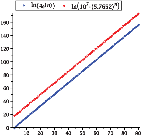
We compare the numbers of \documentclass{aastex}\usepackage{amsbsy}\usepackage{amsfonts}\usepackage{amssymb}\usepackage{bm}\usepackage{mathrsfs}\usepackage{pifont}\usepackage{stmaryrd}\usepackage{textcomp}\usepackage{portland, xspace}\usepackage{amsmath, amsxtra}\pagestyle{empty}\DeclareMathSizes{10}{9}{7}{6}\begin{document}$${\cal Q}_0$$\end{document} -matchings (q₀(n)) versus the asymptotic formula constant 5.7652ⁿ. For representational purposes, we separate the two datasets by setting the constant to 10⁷.

In the case of γ = 1, let δ₁ denote the dominant real singularity of \documentclass{aastex}\usepackage{amsbsy}\usepackage{amsfonts}\usepackage{amssymb}\usepackage{bm}\usepackage{mathrsfs}\usepackage{pifont}\usepackage{stmaryrd}\usepackage{textcomp}\usepackage{portland, xspace}\usepackage{amsmath, amsxtra}\pagestyle{empty}\DeclareMathSizes{10}{9}{7}{6}\begin{document}\begin{align} \textbf{Q} _ {1} ( u ) = \textbf{H} _ {1} ^ {2} ( u ) \cdot \frac {u \textbf{H} ^ {2} _ {1} ( u ) + \sum_ {g \leq 1} \textbf{I} _ {g , 2} \left( \frac {u \cdot \textbf{H} _ {1} ^ {2} ( u )} {1 - u \cdot \textbf{H} _ {1} ^ {2} ( u )} \right)} {1 - u \textbf{H} _ {1} ^ {2} ( u ) - \sum_ {g \leq 1} \textbf{I} _ {g , 2} \left( \frac {u \cdot \textbf{H} _ {1} ^ {2} ( u )} {1 - u \cdot \textbf{H} _ {1} ^ {2} ( u )} \right)} , \tag {3.12} \end{align}\end{document}

whose existence is implied by Pfringsheim's theorem. According to Theorem 2 (Han and Reidys, 2012), H₁(u) has its unique dominant singularity μ₁ at ≈0.1207.

We set \documentclass{aastex}\usepackage{amsbsy}\usepackage{amsfonts}\usepackage{amssymb}\usepackage{bm}\usepackage{mathrsfs}\usepackage{pifont}\usepackage{stmaryrd}\usepackage{textcomp}\usepackage{portland, xspace}\usepackage{amsmath, amsxtra}\pagestyle{empty}\DeclareMathSizes{10}{9}{7}{6}\begin{document}\begin{align} \textbf{N} _ {1} ( u ) = u \textbf{H} ^ {2} _ {1} ( u ) + \sum_ {g \leq 1} \textbf{I} _ {g , 2} \left( \frac {u \cdot \textbf{H} _ {1} ^ {2} ( u )} {1 - u \cdot \textbf{H} _ {1} ^ {2} ( u )} \right) , \ \ \textbf{N} _ {2} ( u ) = \frac {u} {1 - u} . \tag {3.13} \end{align}\end{document}

Since N₁(u) and N₂(u) are power series with non-negative coefficients and in addition N₁(0) = 0, N₃(u) =N₂(N₁(u)) is a well-defined power series. Therefore, Pfringsheim's theorem gives rise to the existence of the dominant singularity of N₃(u), denoted by ρ(N₃(u)). Therefore, Equation (3.12) can be written as \documentclass{aastex}\usepackage{amsbsy}\usepackage{amsfonts}\usepackage{amssymb}\usepackage{bm}\usepackage{mathrsfs}\usepackage{pifont}\usepackage{stmaryrd}\usepackage{textcomp}\usepackage{portland, xspace}\usepackage{amsmath, amsxtra}\pagestyle{empty}\DeclareMathSizes{10}{9}{7}{6}\begin{document}$$\textbf{Q}_{1} ( u ) = \textbf{H}_{1}^{2} ( u ) \cdot \textbf{N}_{2} ( \textbf{N}_{1} ( u ) )$$\end{document} . By construction, we derive \documentclass{aastex}\usepackage{amsbsy}\usepackage{amsfonts}\usepackage{amssymb}\usepackage{bm}\usepackage{mathrsfs}\usepackage{pifont}\usepackage{stmaryrd}\usepackage{textcomp}\usepackage{portland, xspace}\usepackage{amsmath, amsxtra}\pagestyle{empty}\DeclareMathSizes{10}{9}{7}{6}\begin{document}$$\delta_1 = \rho_{\textbf{N}_{3} ( u )}$$\end{document} since \documentclass{aastex}\usepackage{amsbsy}\usepackage{amsfonts}\usepackage{amssymb}\usepackage{bm}\usepackage{mathrsfs}\usepackage{pifont}\usepackage{stmaryrd}\usepackage{textcomp}\usepackage{portland, xspace}\usepackage{amsmath, amsxtra}\pagestyle{empty}\DeclareMathSizes{10}{9}{7}{6}\begin{document}$$\mu_1 = \rho_{\textbf{H}_{1}^{2} ( u )} \geq \rho_{\textbf{N}_{3} ( u )}$$\end{document} and \documentclass{aastex}\usepackage{amsbsy}\usepackage{amsfonts}\usepackage{amssymb}\usepackage{bm}\usepackage{mathrsfs}\usepackage{pifont}\usepackage{stmaryrd}\usepackage{textcomp}\usepackage{portland, xspace}\usepackage{amsmath, amsxtra}\pagestyle{empty}\DeclareMathSizes{10}{9}{7}{6}\begin{document}$$\delta_1 = \textbf{min} \{ \rho_{\textbf{H}_{1}^{2} ( u )} , \rho_{\textbf{N}_{3} ( u )} \} $$\end{document} , where \documentclass{aastex}\usepackage{amsbsy}\usepackage{amsfonts}\usepackage{amssymb}\usepackage{bm}\usepackage{mathrsfs}\usepackage{pifont}\usepackage{stmaryrd}\usepackage{textcomp}\usepackage{portland, xspace}\usepackage{amsmath, amsxtra}\pagestyle{empty}\DeclareMathSizes{10}{9}{7}{6}\begin{document}$$\rho_{\textbf{H}_{1}^{2} ( u )}$$\end{document} is the dominant singularity of the function \documentclass{aastex}\usepackage{amsbsy}\usepackage{amsfonts}\usepackage{amssymb}\usepackage{bm}\usepackage{mathrsfs}\usepackage{pifont}\usepackage{stmaryrd}\usepackage{textcomp}\usepackage{portland, xspace}\usepackage{amsmath, amsxtra}\pagestyle{empty}\DeclareMathSizes{10}{9}{7}{6}\begin{document}$$\textbf{H}_1^2 ( u )$$\end{document} .

To derive \documentclass{aastex}\usepackage{amsbsy}\usepackage{amsfonts}\usepackage{amssymb}\usepackage{bm}\usepackage{mathrsfs}\usepackage{pifont}\usepackage{stmaryrd}\usepackage{textcomp}\usepackage{portland, xspace}\usepackage{amsmath, amsxtra}\pagestyle{empty}\DeclareMathSizes{10}{9}{7}{6}\begin{document}$$\rho_{\textbf{N}_{3} ( u )}$$\end{document} , we need to distinguish the composition paradigm as follows. By construction, there exists \documentclass{aastex}\usepackage{amsbsy}\usepackage{amsfonts}\usepackage{amssymb}\usepackage{bm}\usepackage{mathrsfs}\usepackage{pifont}\usepackage{stmaryrd}\usepackage{textcomp}\usepackage{portland, xspace}\usepackage{amsmath, amsxtra}\pagestyle{empty}\DeclareMathSizes{10}{9}{7}{6}\begin{document}$$\rho_{\textbf{N}_1} = \textbf{min} \{ \rho_{\textbf{H}^{2}_{1} ( u )} , \textbf{Zero} ( u\textbf{H}_{1}^{2} ( u ) = 1 ) \} $$\end{document} . In case of \documentclass{aastex}\usepackage{amsbsy}\usepackage{amsfonts}\usepackage{amssymb}\usepackage{bm}\usepackage{mathrsfs}\usepackage{pifont}\usepackage{stmaryrd}\usepackage{textcomp}\usepackage{portland, xspace}\usepackage{amsmath, amsxtra}\pagestyle{empty}\DeclareMathSizes{10}{9}{7}{6}\begin{document}$$\rho_{\textbf{N}_{1}} = \rho_{\textbf{H}^{2}_{\gamma} ( u )}$$\end{document} , we observe \documentclass{aastex}\usepackage{amsbsy}\usepackage{amsfonts}\usepackage{amssymb}\usepackage{bm}\usepackage{mathrsfs}\usepackage{pifont}\usepackage{stmaryrd}\usepackage{textcomp}\usepackage{portland, xspace}\usepackage{amsmath, amsxtra}\pagestyle{empty}\DeclareMathSizes{10}{9}{7}{6}\begin{document}$$ \textbf{N} _1 ( \frac {2} {17} ) > 1$$\end{document} , which implies that there exists some smallest \documentclass{aastex}\usepackage{amsbsy}\usepackage{amsfonts}\usepackage{amssymb}\usepackage{bm}\usepackage{mathrsfs}\usepackage{pifont}\usepackage{stmaryrd}\usepackage{textcomp}\usepackage{portland, xspace}\usepackage{amsmath, amsxtra}\pagestyle{empty}\DeclareMathSizes{10}{9}{7}{6}\begin{document}$$\delta_ {1} \in ( 0 , \frac {2} {17} )$$\end{document} such that N₁(δ₁) = 1 since N₁(u) is increasing in [0, 2/17] and N₁(0) = 0. Since μ₁ > 2/17 > δ₁, the composition power series N₂(N₁(u)) belongs to the supercritical paradigm (Flajolet and Sedgewick, 2009), that is, its singular expansion is that of the outer function whose dominant singularity is encountered first. Otherwise, in case of \documentclass{aastex}\usepackage{amsbsy}\usepackage{amsfonts}\usepackage{amssymb}\usepackage{bm}\usepackage{mathrsfs}\usepackage{pifont}\usepackage{stmaryrd}\usepackage{textcomp}\usepackage{portland, xspace}\usepackage{amsmath, amsxtra}\pagestyle{empty}\DeclareMathSizes{10}{9}{7}{6}\begin{document}$$\rho_{\textbf{N}_{1}} \in \textbf{Zero} ( u\textbf{H}^{2} ( u ) = 1 )$$\end{document} , N₂(N₁(u)) still belongs to the supercritical paradigm since \documentclass{aastex}\usepackage{amsbsy}\usepackage{amsfonts}\usepackage{amssymb}\usepackage{bm}\usepackage{mathrsfs}\usepackage{pifont}\usepackage{stmaryrd}\usepackage{textcomp}\usepackage{portland, xspace}\usepackage{amsmath, amsxtra}\pagestyle{empty}\DeclareMathSizes{10}{9}{7}{6}\begin{document}$$\textbf{N}_{1} ( u ) > u\textbf{H}^{2}_{1} ( u )$$\end{document} and \documentclass{aastex}\usepackage{amsbsy}\usepackage{amsfonts}\usepackage{amssymb}\usepackage{bm}\usepackage{mathrsfs}\usepackage{pifont}\usepackage{stmaryrd}\usepackage{textcomp}\usepackage{portland, xspace}\usepackage{amsmath, amsxtra}\pagestyle{empty}\DeclareMathSizes{10}{9}{7}{6}\begin{document}$$u\textbf{H}^{2}_{1} ( u )$$\end{document} is increasing when u > 0, which leads to the fact that N₁(u) hits value 1 earlier than \documentclass{aastex}\usepackage{amsbsy}\usepackage{amsfonts}\usepackage{amssymb}\usepackage{bm}\usepackage{mathrsfs}\usepackage{pifont}\usepackage{stmaryrd}\usepackage{textcomp}\usepackage{portland, xspace}\usepackage{amsmath, amsxtra}\pagestyle{empty}\DeclareMathSizes{10}{9}{7}{6}\begin{document}$$u\textbf{H}^{2}_{1} ( u )$$\end{document} . This evidently is the singular expansion of N₃(u) leading (again) to the subexponential factor of 1. Using Maple command fsolve, we find δ₁ ≈ 0.11173 < μ₁ and derive \documentclass{aastex}\usepackage{amsbsy}\usepackage{amsfonts}\usepackage{amssymb}\usepackage{bm}\usepackage{mathrsfs}\usepackage{pifont}\usepackage{stmaryrd}\usepackage{textcomp}\usepackage{portland, xspace}\usepackage{amsmath, amsxtra}\pagestyle{empty}\DeclareMathSizes{10}{9}{7}{6}\begin{document}\begin{align}[ u^n ] \textbf{N}_{3} ( u ) = c_1 \cdot \delta_{1}^{- n} \approx c \cdot \left( 8.9499 \right) ^n , \tag{3.14}\end{align}\end{document}

for some c > 0 and consequently \documentclass{aastex}\usepackage{amsbsy}\usepackage{amsfonts}\usepackage{amssymb}\usepackage{bm}\usepackage{mathrsfs}\usepackage{pifont}\usepackage{stmaryrd}\usepackage{textcomp}\usepackage{portland, xspace}\usepackage{amsmath, amsxtra}\pagestyle{empty}\DeclareMathSizes{10}{9}{7}{6}\begin{document}\begin{align}[ u^n ] \textbf{Q}_{1} ( u ) k_{1} \cdot \delta_{1}^{- n} \approx k_{1} \cdot \left( 8.9499 \right) ^n , \tag{3.15}\end{align}\end{document}

where k₁ is some positive constant. This completes the proof of the theorem. ■

4. γ-Interaction Structures

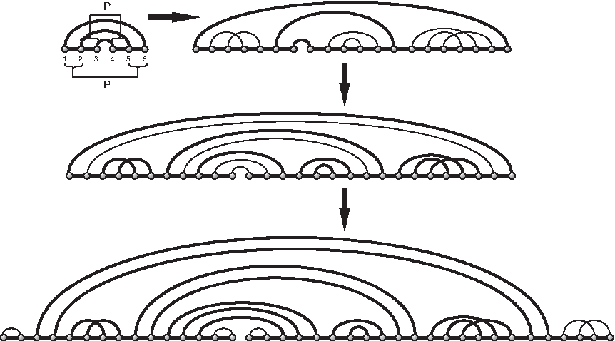
The enumeration of γ-interaction structures is obtained using shapes. A matching X is a shape if each stack in X is exactly length one. Given an arbitrary matching s, its shape is obtained by iteratively collapsing each stack to a single arc and then removing any isolated vertices from the obtained diagram as illustrated in Figure 14.

FIG. 14.
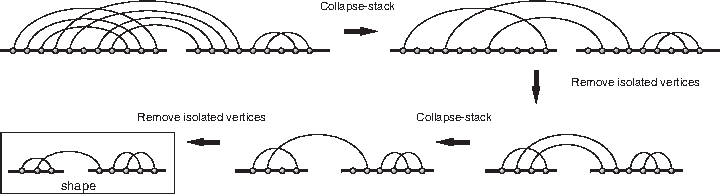
From a diagram to its shape.

Let \documentclass{aastex}\usepackage{amsbsy}\usepackage{amsfonts}\usepackage{amssymb}\usepackage{bm}\usepackage{mathrsfs}\usepackage{pifont}\usepackage{stmaryrd}\usepackage{textcomp}\usepackage{portland, xspace}\usepackage{amsmath, amsxtra}\pagestyle{empty}\DeclareMathSizes{10}{9}{7}{6}\begin{document}$${\cal S}_{\gamma}$$\end{document} denote the set of shapes that are \documentclass{aastex}\usepackage{amsbsy}\usepackage{amsfonts}\usepackage{amssymb}\usepackage{bm}\usepackage{mathrsfs}\usepackage{pifont}\usepackage{stmaryrd}\usepackage{textcomp}\usepackage{portland, xspace}\usepackage{amsmath, amsxtra}\pagestyle{empty}\DeclareMathSizes{10}{9}{7}{6}\begin{document}$${\cal Q}_{\gamma}$$\end{document} -matchings, and let \documentclass{aastex}\usepackage{amsbsy}\usepackage{amsfonts}\usepackage{amssymb}\usepackage{bm}\usepackage{mathrsfs}\usepackage{pifont}\usepackage{stmaryrd}\usepackage{textcomp}\usepackage{portland, xspace}\usepackage{amsmath, amsxtra}\pagestyle{empty}\DeclareMathSizes{10}{9}{7}{6}\begin{document}$${\cal Q}_{\gamma} ( n , m )$$\end{document} denote the combinatorial class of \documentclass{aastex}\usepackage{amsbsy}\usepackage{amsfonts}\usepackage{amssymb}\usepackage{bm}\usepackage{mathrsfs}\usepackage{pifont}\usepackage{stmaryrd}\usepackage{textcomp}\usepackage{portland, xspace}\usepackage{amsmath, amsxtra}\pagestyle{empty}\DeclareMathSizes{10}{9}{7}{6}\begin{document}$${\cal Q}_{\gamma}$$\end{document} -matchings over 2n vertices with m interior arcs of length 1 (1-arcs). Note that any 1-arc is by definition an interior arc. Furthermore, let \documentclass{aastex}\usepackage{amsbsy}\usepackage{amsfonts}\usepackage{amssymb}\usepackage{bm}\usepackage{mathrsfs}\usepackage{pifont}\usepackage{stmaryrd}\usepackage{textcomp}\usepackage{portland, xspace}\usepackage{amsmath, amsxtra}\pagestyle{empty}\DeclareMathSizes{10}{9}{7}{6}\begin{document}$${\cal S}_{\gamma} ( n , m )$$\end{document} denote the class of all \documentclass{aastex}\usepackage{amsbsy}\usepackage{amsfonts}\usepackage{amssymb}\usepackage{bm}\usepackage{mathrsfs}\usepackage{pifont}\usepackage{stmaryrd}\usepackage{textcomp}\usepackage{portland, xspace}\usepackage{amsmath, amsxtra}\pagestyle{empty}\DeclareMathSizes{10}{9}{7}{6}\begin{document}$${\cal S}_{\gamma}$$\end{document} -shapes over 2n vertices with m 1-arcs with generating function S_γ(u, e).

Lemma 2

For any γ ≥ 0, we have \documentclass{aastex}\usepackage{amsbsy}\usepackage{amsfonts}\usepackage{amssymb}\usepackage{bm}\usepackage{mathrsfs}\usepackage{pifont}\usepackage{stmaryrd}\usepackage{textcomp}\usepackage{portland, xspace}\usepackage{amsmath, amsxtra}\pagestyle{empty}\DeclareMathSizes{10}{9}{7}{6}\begin{document}\begin{align} \textbf{S} _ {\gamma} ( u , e ) = \frac {( 1 + u ) ^ {2}} {( 1 + 2u - ue ) ^ {2}} \textbf{Q} _ {\gamma} \left( \frac {u ( 1 + u )} {( 1 + 2u - ue ) ^2} \right). \tag {4.1} \end{align}\end{document}

Proof. First we claim that \documentclass{aastex}\usepackage{amsbsy}\usepackage{amsfonts}\usepackage{amssymb}\usepackage{bm}\usepackage{mathrsfs}\usepackage{pifont}\usepackage{stmaryrd}\usepackage{textcomp}\usepackage{portland, xspace}\usepackage{amsmath, amsxtra}\pagestyle{empty}\DeclareMathSizes{10}{9}{7}{6}\begin{document}\begin{align} \textbf{Q} _ {\gamma} ( x , y ) = \frac {1} {( x + 1 - yx ) ^ {2}} \textbf{Q} _ {\gamma} \left( \frac {x} {( x + 1 - yx ) ^2} \right). \tag {4.2} \end{align}\end{document}

Consider the number of all possible \documentclass{aastex}\usepackage{amsbsy}\usepackage{amsfonts}\usepackage{amssymb}\usepackage{bm}\usepackage{mathrsfs}\usepackage{pifont}\usepackage{stmaryrd}\usepackage{textcomp}\usepackage{portland, xspace}\usepackage{amsmath, amsxtra}\pagestyle{empty}\DeclareMathSizes{10}{9}{7}{6}\begin{document}$${\cal Q}_{\gamma} ( s + 1 , m + 1 )$$\end{document} -matchings with exactly one labeled 1-arc. There are two ways to enumerate this. On one hand, choose an arbitrary \documentclass{aastex}\usepackage{amsbsy}\usepackage{amsfonts}\usepackage{amssymb}\usepackage{bm}\usepackage{mathrsfs}\usepackage{pifont}\usepackage{stmaryrd}\usepackage{textcomp}\usepackage{portland, xspace}\usepackage{amsmath, amsxtra}\pagestyle{empty}\DeclareMathSizes{10}{9}{7}{6}\begin{document}$$\xi \in {\cal Q}_{\gamma} ( s + 1 , m + 1 )$$\end{document} and label one of its 1-arcs. Since we can label any of the (m + 1) 1-arcs of ξ, (m + 1) h_γ(s + 1, m + 1) different such labeled linear arc diagrams arise. On the other hand, to produce ξ with this labeling, we can add one labeled 1-arc to an element of \documentclass{aastex}\usepackage{amsbsy}\usepackage{amsfonts}\usepackage{amssymb}\usepackage{bm}\usepackage{mathrsfs}\usepackage{pifont}\usepackage{stmaryrd}\usepackage{textcomp}\usepackage{portland, xspace}\usepackage{amsmath, amsxtra}\pagestyle{empty}\DeclareMathSizes{10}{9}{7}{6}\begin{document}$${\cal Q}_{\gamma} ( s , m + 1 )$$\end{document} by inserting a parallel copy of an existing 1-arcs or by inserting a new labeled 1-arc into an element of \documentclass{aastex}\usepackage{amsbsy}\usepackage{amsfonts}\usepackage{amssymb}\usepackage{bm}\usepackage{mathrsfs}\usepackage{pifont}\usepackage{stmaryrd}\usepackage{textcomp}\usepackage{portland, xspace}\usepackage{amsmath, amsxtra}\pagestyle{empty}\DeclareMathSizes{10}{9}{7}{6}\begin{document}$${\cal Q}_{\gamma} ( s , m )$$\end{document} , where we may only insert the 1-arc between two vertices not already forming a 1-arc. It follows that we have the recursion \documentclass{aastex}\usepackage{amsbsy}\usepackage{amsfonts}\usepackage{amssymb}\usepackage{bm}\usepackage{mathrsfs}\usepackage{pifont}\usepackage{stmaryrd}\usepackage{textcomp}\usepackage{portland, xspace}\usepackage{amsmath, amsxtra}\pagestyle{empty}\DeclareMathSizes{10}{9}{7}{6}\begin{document}\begin{align}( m + 1 ) \,\textbf{q}_ \gamma ( n + 1 , m + 1 ) = ( m + 1 ) \,\textbf{q}_ \gamma ( n , m + 1 ) + ( 2n + 2 - m ) \,\textbf{q}_ \gamma ( n , m )\end{align}\end{document}

or equivalently the PDE \documentclass{aastex}\usepackage{amsbsy}\usepackage{amsfonts}\usepackage{amssymb}\usepackage{bm}\usepackage{mathrsfs}\usepackage{pifont}\usepackage{stmaryrd}\usepackage{textcomp}\usepackage{portland, xspace}\usepackage{amsmath, amsxtra}\pagestyle{empty}\DeclareMathSizes{10}{9}{7}{6}\begin{document}\begin{align} \frac {\partial \textbf{Q} _ \gamma ( x , y )} {\partial y} = x \frac {\partial \textbf{Q} _ \gamma ( x , y )} {\partial y} + 2x^2 \frac {\partial \textbf{Q} _ \gamma ( x , y )} {\partial x} + 2x \textbf{Q} _ \gamma ( x , y ) - xy \frac {\partial \textbf{Q} _ \gamma ( x , y )} {\partial y} , \tag {4.3} \end{align}\end{document}

which is thus satisfied by Q_γ(x, y).

On the other hand, \documentclass{aastex}\usepackage{amsbsy}\usepackage{amsfonts}\usepackage{amssymb}\usepackage{bm}\usepackage{mathrsfs}\usepackage{pifont}\usepackage{stmaryrd}\usepackage{textcomp}\usepackage{portland, xspace}\usepackage{amsmath, amsxtra}\pagestyle{empty}\DeclareMathSizes{10}{9}{7}{6}\begin{document}\begin{align} \textbf{Q} ^_ \gamma ( x , y ) = \frac {1} {( x + 1 - yx ) ^2} \textbf{Q} _ \gamma \left( \frac {x} {( x + 1 - yx ) ^2} \right)\end{align}\end{document}

is also a solution of Equation (4.3), which specializes to \documentclass{aastex}\usepackage{amsbsy}\usepackage{amsfonts}\usepackage{amssymb}\usepackage{bm}\usepackage{mathrsfs}\usepackage{pifont}\usepackage{stmaryrd}\usepackage{textcomp}\usepackage{portland, xspace}\usepackage{amsmath, amsxtra}\pagestyle{empty}\DeclareMathSizes{10}{9}{7}{6}\begin{document}$$\textbf{Q}_{\gamma} ( x ) = \textbf{Q}_{\gamma}^ ( x , 1 )$$\end{document} , and moreover, we have \documentclass{aastex}\usepackage{amsbsy}\usepackage{amsfonts}\usepackage{amssymb}\usepackage{bm}\usepackage{mathrsfs}\usepackage{pifont}\usepackage{stmaryrd}\usepackage{textcomp}\usepackage{portland, xspace}\usepackage{amsmath, amsxtra}\pagestyle{empty}\DeclareMathSizes{10}{9}{7}{6}\begin{document}$$\textbf{q}_{\gamma}^* ( n , m ) = [ x^ny^m ] \textbf{Q}_{\gamma}^* ( x , y ) = 0$$\end{document} , for m > n. Indeed, the first assertion is easily verified directly, the specialization is obvious, and the fact that y only appears in the power series \documentclass{aastex}\usepackage{amsbsy}\usepackage{amsfonts}\usepackage{amssymb}\usepackage{bm}\usepackage{mathrsfs}\usepackage{pifont}\usepackage{stmaryrd}\usepackage{textcomp}\usepackage{portland, xspace}\usepackage{amsmath, amsxtra}\pagestyle{empty}\DeclareMathSizes{10}{9}{7}{6}\begin{document}$$\textbf{Q}_{\gamma}^* ( x , y )$$\end{document} in the form of products xy implies that \documentclass{aastex}\usepackage{amsbsy}\usepackage{amsfonts}\usepackage{amssymb}\usepackage{bm}\usepackage{mathrsfs}\usepackage{pifont}\usepackage{stmaryrd}\usepackage{textcomp}\usepackage{portland, xspace}\usepackage{amsmath, amsxtra}\pagestyle{empty}\DeclareMathSizes{10}{9}{7}{6}\begin{document}$$\textbf{q}_{\gamma}^* ( n , m ) = 0$$\end{document} , for m > n. Thus, the coefficients \documentclass{aastex}\usepackage{amsbsy}\usepackage{amsfonts}\usepackage{amssymb}\usepackage{bm}\usepackage{mathrsfs}\usepackage{pifont}\usepackage{stmaryrd}\usepackage{textcomp}\usepackage{portland, xspace}\usepackage{amsmath, amsxtra}\pagestyle{empty}\DeclareMathSizes{10}{9}{7}{6}\begin{document}$$\textbf{q}_{\gamma}^* ( n , m )$$\end{document} satisfy the same recursion and initial conditions as q_γ(n, m), and hence by induction on n, we conclude \documentclass{aastex}\usepackage{amsbsy}\usepackage{amsfonts}\usepackage{amssymb}\usepackage{bm}\usepackage{mathrsfs}\usepackage{pifont}\usepackage{stmaryrd}\usepackage{textcomp}\usepackage{portland, xspace}\usepackage{amsmath, amsxtra}\pagestyle{empty}\DeclareMathSizes{10}{9}{7}{6}\begin{document}$$\textbf{q}_{\gamma}^* ( n , m ) = \textbf{q}_{\gamma} ( n , m )$$\end{document} , for n, m ≥ 0. This proves that Q_γ(n, m) indeed satisfies Equation (4.2) as was claimed.

To complete the proof of Equation (4.1), we will define a projection \documentclass{aastex}\usepackage{amsbsy}\usepackage{amsfonts}\usepackage{amssymb}\usepackage{bm}\usepackage{mathrsfs}\usepackage{pifont}\usepackage{stmaryrd}\usepackage{textcomp}\usepackage{portland, xspace}\usepackage{amsmath, amsxtra}\pagestyle{empty}\DeclareMathSizes{10}{9}{7}{6}\begin{document}\begin{align}\vartheta: \ {\cal Q}_{\gamma} \rightarrow {\cal S}_{\gamma} ,\end{align}\end{document}

which projects an arbitrary \documentclass{aastex}\usepackage{amsbsy}\usepackage{amsfonts}\usepackage{amssymb}\usepackage{bm}\usepackage{mathrsfs}\usepackage{pifont}\usepackage{stmaryrd}\usepackage{textcomp}\usepackage{portland, xspace}\usepackage{amsmath, amsxtra}\pagestyle{empty}\DeclareMathSizes{10}{9}{7}{6}\begin{document}$${\cal Q}_{\gamma}$$\end{document} -matching s into its unique shape s. Clearly, ϑ is surjective and affects neither irreducible shadows nor the number of 1-arcs. It can be naturally restricted to \documentclass{aastex}\usepackage{amsbsy}\usepackage{amsfonts}\usepackage{amssymb}\usepackage{bm}\usepackage{mathrsfs}\usepackage{pifont}\usepackage{stmaryrd}\usepackage{textcomp}\usepackage{portland, xspace}\usepackage{amsmath, amsxtra}\pagestyle{empty}\DeclareMathSizes{10}{9}{7}{6}\begin{document}\begin{align}\vartheta_m: \bigcup_{n}{\cal Q}_{\gamma} ( n , m ) \rightarrow \bigcup_{n}{\cal S}_{\gamma} ( n , m ).\end{align}\end{document}

Let us consider a fixed γ-shape, λ, having s arcs, of which t are 1-arcs and the generating function \documentclass{aastex}\usepackage{amsbsy}\usepackage{amsfonts}\usepackage{amssymb}\usepackage{bm}\usepackage{mathrsfs}\usepackage{pifont}\usepackage{stmaryrd}\usepackage{textcomp}\usepackage{portland, xspace}\usepackage{amsmath, amsxtra}\pagestyle{empty}\DeclareMathSizes{10}{9}{7}{6}\begin{document}$$\textbf{Q}_{\gamma}^{\lambda} ( x , y )$$\end{document} , counting γ-matchings that project into λ via ϑ_m. Then \documentclass{aastex}\usepackage{amsbsy}\usepackage{amsfonts}\usepackage{amssymb}\usepackage{bm}\usepackage{mathrsfs}\usepackage{pifont}\usepackage{stmaryrd}\usepackage{textcomp}\usepackage{portland, xspace}\usepackage{amsmath, amsxtra}\pagestyle{empty}\DeclareMathSizes{10}{9}{7}{6}\begin{document}\begin{align} \textbf{Q} _ {\gamma} ^ {\lambda} ( x , y ) = \left( \frac {x} {1 - x} \right) ^s y^t ,\end{align}\end{document}

which shows that \documentclass{aastex}\usepackage{amsbsy}\usepackage{amsfonts}\usepackage{amssymb}\usepackage{bm}\usepackage{mathrsfs}\usepackage{pifont}\usepackage{stmaryrd}\usepackage{textcomp}\usepackage{portland, xspace}\usepackage{amsmath, amsxtra}\pagestyle{empty}\DeclareMathSizes{10}{9}{7}{6}\begin{document}$$\textbf{Q}_{\gamma}^{\lambda} ( x , y )$$\end{document} depends only on the total number of arcs and number of 1-arcs in λ. Consequently, \documentclass{aastex}\usepackage{amsbsy}\usepackage{amsfonts}\usepackage{amssymb}\usepackage{bm}\usepackage{mathrsfs}\usepackage{pifont}\usepackage{stmaryrd}\usepackage{textcomp}\usepackage{portland, xspace}\usepackage{amsmath, amsxtra}\pagestyle{empty}\DeclareMathSizes{10}{9}{7}{6}\begin{document}\begin{align} \textbf{Q} _ \gamma ( x , y ) = \sum_ {s \geq 0} \sum_ {m = 0} ^ {s} \textbf{s} _ \gamma ( s , m ) \left( \frac {x} {1 - x} \right)^sy^m = \textbf{S} _ \gamma \left( \frac {x} {1 - x} , y \right). \tag {4.4} \end{align}\end{document}

Setting \documentclass{aastex}\usepackage{amsbsy}\usepackage{amsfonts}\usepackage{amssymb}\usepackage{bm}\usepackage{mathrsfs}\usepackage{pifont}\usepackage{stmaryrd}\usepackage{textcomp}\usepackage{portland, xspace}\usepackage{amsmath, amsxtra}\pagestyle{empty}\DeclareMathSizes{10}{9}{7}{6}\begin{document}$$u = \frac {x} {1 - x} $$\end{document} , that is, \documentclass{aastex}\usepackage{amsbsy}\usepackage{amsfonts}\usepackage{amssymb}\usepackage{bm}\usepackage{mathrsfs}\usepackage{pifont}\usepackage{stmaryrd}\usepackage{textcomp}\usepackage{portland, xspace}\usepackage{amsmath, amsxtra}\pagestyle{empty}\DeclareMathSizes{10}{9}{7}{6}\begin{document}$$x = \frac {u} {1 + u} $$\end{document} , and e = y, we arrive at \documentclass{aastex}\usepackage{amsbsy}\usepackage{amsfonts}\usepackage{amssymb}\usepackage{bm}\usepackage{mathrsfs}\usepackage{pifont}\usepackage{stmaryrd}\usepackage{textcomp}\usepackage{portland, xspace}\usepackage{amsmath, amsxtra}\pagestyle{empty}\DeclareMathSizes{10}{9}{7}{6}\begin{document}\begin{align} \textbf{S} _ {\gamma} ( u , e ) = \frac {( 1 + u ) ^ {2}} {( 1 + 2u - ue ) ^ {2}} \textbf{Q} _ {\gamma} \left( \frac {u ( 1 + u )} {( 1 + 2u - ue ) ^2} \right) ,\end{align}\end{document}

as required. ■

Using symbolic enumeration we can conclude from Lemma 2:

Lemma 3

Let λ be a fixed γ-shape with s* ≥ 1 arcs and m ≥ 0 1-arcs. Then the generating function of τ-canonical γ-diagrams containing no 1-arc that have shape λ is given by \documentclass{aastex}\usepackage{amsbsy}\usepackage{amsfonts}\usepackage{amssymb}\usepackage{bm}\usepackage{mathrsfs}\usepackage{pifont}\usepackage{stmaryrd}\usepackage{textcomp}\usepackage{portland, xspace}\usepackage{amsmath, amsxtra}\pagestyle{empty}\DeclareMathSizes{10}{9}{7}{6}\begin{document}\begin{align} \textbf{Q} ^ {\lambda} _ {\tau , \gamma} ( z ) = ( 1 - z ) ^ {- 2} \left( \frac {z^ {2 \tau}} {( 1 - z^2 ) ( 1 - z ) ^2 - ( 2z - z^2 ) z^ {2 \tau}} \right) ^s \ z^m.\end{align}\end{document}

In particular, \documentclass{aastex}\usepackage{amsbsy}\usepackage{amsfonts}\usepackage{amssymb}\usepackage{bm}\usepackage{mathrsfs}\usepackage{pifont}\usepackage{stmaryrd}\usepackage{textcomp}\usepackage{portland, xspace}\usepackage{amsmath, amsxtra}\pagestyle{empty}\DeclareMathSizes{10}{9}{7}{6}\begin{document}$$\textbf{Q}_{\tau , \gamma}^{\lambda} ( z )$$\end{document} depends only upon the number of arcs and 1-arcs in λ.

Proof. Given λ, we can construct an arbitrary τ-canonical γ-diagram containing no 1-arc that has shape λ by the following steps:
• We start from the diagram λ, insert at most one isolated vertex after each given vertices \documentclass{aastex}\usepackage{amsbsy}\usepackage{amsfonts}\usepackage{amssymb}\usepackage{bm}\usepackage{mathrsfs}\usepackage{pifont}\usepackage{stmaryrd}\usepackage{textcomp}\usepackage{portland, xspace}\usepackage{amsmath, amsxtra}\pagestyle{empty}\DeclareMathSizes{10}{9}{7}{6}\begin{document}$$i \in [ 2s ]$$\end{document} together except the vertices j such that (j, j + 1) forming a 1-arc in λ. In case i is at the end of the backbone, we furthermore prolong the backbone to connect i with the inserted isolated vertex. The obtained combinatorial class is symbolically given by \documentclass{aastex}\usepackage{amsbsy}\usepackage{amsfonts}\usepackage{amssymb}\usepackage{bm}\usepackage{mathrsfs}\usepackage{pifont}\usepackage{stmaryrd}\usepackage{textcomp}\usepackage{portland, xspace}\usepackage{amsmath, amsxtra}\pagestyle{empty}\DeclareMathSizes{10}{9}{7}{6}\begin{document}$${\cal M}_1 = {\cal U}^{s} \times ( {\cal E} + {\cal {Z}} ) ^{2s - m}$$\end{document} .

• We insert at most one isolated vertex before the first vertex of the backbones. The obtained combinatorial class is symbolically given by \documentclass{aastex}\usepackage{amsbsy}\usepackage{amsfonts}\usepackage{amssymb}\usepackage{bm}\usepackage{mathrsfs}\usepackage{pifont}\usepackage{stmaryrd}\usepackage{textcomp}\usepackage{portland, xspace}\usepackage{amsmath, amsxtra}\pagestyle{empty}\DeclareMathSizes{10}{9}{7}{6}\begin{document}$${\cal M}_2 = {\cal M}_1 \times ( {\cal E} + {\cal {Z}} ) ^2$$\end{document} .

• We insert exactly one isolated vertex after each vertex j such that (j, j + 1) forms an 1-arc in λ. The obtained combinatorial class is symbolically given by \documentclass{aastex}\usepackage{amsbsy}\usepackage{amsfonts}\usepackage{amssymb}\usepackage{bm}\usepackage{mathrsfs}\usepackage{pifont}\usepackage{stmaryrd}\usepackage{textcomp}\usepackage{portland, xspace}\usepackage{amsmath, amsxtra}\pagestyle{empty}\DeclareMathSizes{10}{9}{7}{6}\begin{document}$${\cal M}_3 = {\cal M}_2 \times {\cal {Z}}^m$$\end{document} .

• We inflate each arc into a stack of length t ≥ 0. In the case of t > 1, assuming \documentclass{aastex}\usepackage{amsbsy}\usepackage{amsfonts}\usepackage{amssymb}\usepackage{bm}\usepackage{mathrsfs}\usepackage{pifont}\usepackage{stmaryrd}\usepackage{textcomp}\usepackage{portland, xspace}\usepackage{amsmath, amsxtra}\pagestyle{empty}\DeclareMathSizes{10}{9}{7}{6}\begin{document}$$S_{i , j}^t$$\end{document} , there are t − 1 pairs of P-intervals of the form ([i + ℓ, i + ℓ + 1], [j − ℓ − 1, j − ℓ]), where \documentclass{aastex}\usepackage{amsbsy}\usepackage{amsfonts}\usepackage{amssymb}\usepackage{bm}\usepackage{mathrsfs}\usepackage{pifont}\usepackage{stmaryrd}\usepackage{textcomp}\usepackage{portland, xspace}\usepackage{amsmath, amsxtra}\pagestyle{empty}\DeclareMathSizes{10}{9}{7}{6}\begin{document}$$\ell \in [ t - 1 ]$$\end{document} . For each pair of P-intervals, we can insert an isolated vertex either to the left, the right, or on both sides in order to separate the arcs. The combinatorial class \documentclass{aastex}\usepackage{amsbsy}\usepackage{amsfonts}\usepackage{amssymb}\usepackage{bm}\usepackage{mathrsfs}\usepackage{pifont}\usepackage{stmaryrd}\usepackage{textcomp}\usepackage{portland, xspace}\usepackage{amsmath, amsxtra}\pagestyle{empty}\DeclareMathSizes{10}{9}{7}{6}\begin{document}$${\cal M}_4$$\end{document} is then symbolically obtained from \documentclass{aastex}\usepackage{amsbsy}\usepackage{amsfonts}\usepackage{amssymb}\usepackage{bm}\usepackage{mathrsfs}\usepackage{pifont}\usepackage{stmaryrd}\usepackage{textcomp}\usepackage{portland, xspace}\usepackage{amsmath, amsxtra}\pagestyle{empty}\DeclareMathSizes{10}{9}{7}{6}\begin{document}$${\cal M}_3$$\end{document} by substitution
\documentclass{aastex}\usepackage{amsbsy}\usepackage{amsfonts}\usepackage{amssymb}\usepackage{bm}\usepackage{mathrsfs}\usepackage{pifont}\usepackage{stmaryrd}\usepackage{textcomp}\usepackage{portland, xspace}\usepackage{amsmath, amsxtra}\pagestyle{empty}\DeclareMathSizes{10}{9}{7}{6}\begin{document}\begin{align}{\cal U} \rightarrow \sum_{t \leq 1} {\cal U}^{t} \times ( 2 {\cal {Z}} + {\cal {Z}}^2 ) ^{t - 1}.\end{align}\end{document}
• We inflate each arc in the obtained structure into a stack of length at least τ. The obtained combinatorial class \documentclass{aastex}\usepackage{amsbsy}\usepackage{amsfonts}\usepackage{amssymb}\usepackage{bm}\usepackage{mathrsfs}\usepackage{pifont}\usepackage{stmaryrd}\usepackage{textcomp}\usepackage{portland, xspace}\usepackage{amsmath, amsxtra}\pagestyle{empty}\DeclareMathSizes{10}{9}{7}{6}\begin{document}$${\cal M}_5$$\end{document} is symbolically obtained from \documentclass{aastex}\usepackage{amsbsy}\usepackage{amsfonts}\usepackage{amssymb}\usepackage{bm}\usepackage{mathrsfs}\usepackage{pifont}\usepackage{stmaryrd}\usepackage{textcomp}\usepackage{portland, xspace}\usepackage{amsmath, amsxtra}\pagestyle{empty}\DeclareMathSizes{10}{9}{7}{6}\begin{document}$${\cal M}_4$$\end{document} by the substitution \documentclass{aastex}\usepackage{amsbsy}\usepackage{amsfonts}\usepackage{amssymb}\usepackage{bm}\usepackage{mathrsfs}\usepackage{pifont}\usepackage{stmaryrd}\usepackage{textcomp}\usepackage{portland, xspace}\usepackage{amsmath, amsxtra}\pagestyle{empty}\DeclareMathSizes{10}{9}{7}{6}\begin{document}$$ {\cal U} \rightarrow \frac {{\cal U} ^ {\tau}} {1 - {\cal U}} $$\end{document} .

• We inflate each isolated vertex into a sequence of isolated vertices of length at least one. The obtained combinatorial class is symbolically obtained from \documentclass{aastex}\usepackage{amsbsy}\usepackage{amsfonts}\usepackage{amssymb}\usepackage{bm}\usepackage{mathrsfs}\usepackage{pifont}\usepackage{stmaryrd}\usepackage{textcomp}\usepackage{portland, xspace}\usepackage{amsmath, amsxtra}\pagestyle{empty}\DeclareMathSizes{10}{9}{7}{6}\begin{document}$${\cal M}_5$$\end{document} by the substitution \documentclass{aastex}\usepackage{amsbsy}\usepackage{amsfonts}\usepackage{amssymb}\usepackage{bm}\usepackage{mathrsfs}\usepackage{pifont}\usepackage{stmaryrd}\usepackage{textcomp}\usepackage{portland, xspace}\usepackage{amsmath, amsxtra}\pagestyle{empty}\DeclareMathSizes{10}{9}{7}{6}\begin{document}$$ {\cal Z} \rightarrow \frac {{\cal Z}} {1 - {\cal Z}} $$\end{document} and the lemma follows. ■

Our main result about enumerating τ-canonical γ-interaction structures follows.

Theorem 5

Suppose γ ≥ 0 and τ ≥ 1 and let \documentclass{aastex}\usepackage{amsbsy}\usepackage{amsfonts}\usepackage{amssymb}\usepackage{bm}\usepackage{mathrsfs}\usepackage{pifont}\usepackage{stmaryrd}\usepackage{textcomp}\usepackage{portland, xspace}\usepackage{amsmath, amsxtra}\pagestyle{empty}\DeclareMathSizes{10}{9}{7}{6}\begin{document}$$u_ \tau ( z ) = \frac {( z^2 ) ^ {\tau - 1}} {z^ {2 \tau} - z^2 + 1} $$\end{document} . Then the generating function Q_τ,γ(z) is algebraic and given by \documentclass{aastex}\usepackage{amsbsy}\usepackage{amsfonts}\usepackage{amssymb}\usepackage{bm}\usepackage{mathrsfs}\usepackage{pifont}\usepackage{stmaryrd}\usepackage{textcomp}\usepackage{portland, xspace}\usepackage{amsmath, amsxtra}\pagestyle{empty}\DeclareMathSizes{10}{9}{7}{6}\begin{document}\begin{align} \textbf{Q} _ {\tau , \gamma} ( z ) = \frac {1} {\left( u_ \tau ( z ) z^ {2} - z + 1 \right) ^2} \ \textbf{Q} _ \gamma \left( \frac {u_ \tau ( z ) z^2} {\left( u_ \tau ( z ) z^ {2} - z + 1 \right) ^2} \right). \tag {4.5} \end{align}\end{document}

In particular, for γ = 0 we have \documentclass{aastex}\usepackage{amsbsy}\usepackage{amsfonts}\usepackage{amssymb}\usepackage{bm}\usepackage{mathrsfs}\usepackage{pifont}\usepackage{stmaryrd}\usepackage{textcomp}\usepackage{portland, xspace}\usepackage{amsmath, amsxtra}\pagestyle{empty}\DeclareMathSizes{10}{9}{7}{6}\begin{document}\begin{align}[ z^n ] \textbf{Q}_{1 , 0} ( z ) \,\sim\, k_{1 , 0} ( \rho_{1 , 0}^{- 1} ) ^n \quad {\rm and} \quad [ z^n ] \textbf{Q}_{2 , 0} ( z )\, \sim\, k_{2 , 0} ( \rho_{2 , 0}^{- 1} ) ^n ,\end{align}\end{document}

and for γ = 1 we have \documentclass{aastex}\usepackage{amsbsy}\usepackage{amsfonts}\usepackage{amssymb}\usepackage{bm}\usepackage{mathrsfs}\usepackage{pifont}\usepackage{stmaryrd}\usepackage{textcomp}\usepackage{portland, xspace}\usepackage{amsmath, amsxtra}\pagestyle{empty}\DeclareMathSizes{10}{9}{7}{6}\begin{document}\begin{align}[ z^n ] \textbf{Q}_{1 , 1} ( z )\, \sim\, k_{1 , 1} ( \rho_{1 , 1}^{- 1} ) ^n \quad {\rm and} \quad [ z^n ] \textbf{Q}_{2 , 1} ( z ) \, \sim\, k_{2 , 1} ( \rho_{2 , 1}^{- 1} ) ^n\end{align}\end{document}

for some constants k₁, k₂, where \documentclass{aastex}\usepackage{amsbsy}\usepackage{amsfonts}\usepackage{amssymb}\usepackage{bm}\usepackage{mathrsfs}\usepackage{pifont}\usepackage{stmaryrd}\usepackage{textcomp}\usepackage{portland, xspace}\usepackage{amsmath, amsxtra}\pagestyle{empty}\DeclareMathSizes{10}{9}{7}{6}\begin{document}$$\rho_{1 , 0}^{- 1} = 3.0760$$\end{document} , \documentclass{aastex}\usepackage{amsbsy}\usepackage{amsfonts}\usepackage{amssymb}\usepackage{bm}\usepackage{mathrsfs}\usepackage{pifont}\usepackage{stmaryrd}\usepackage{textcomp}\usepackage{portland, xspace}\usepackage{amsmath, amsxtra}\pagestyle{empty}\DeclareMathSizes{10}{9}{7}{6}\begin{document}$$\rho_{2 , 0}^{- 1} = 2.1190$$\end{document} , \documentclass{aastex}\usepackage{amsbsy}\usepackage{amsfonts}\usepackage{amssymb}\usepackage{bm}\usepackage{mathrsfs}\usepackage{pifont}\usepackage{stmaryrd}\usepackage{textcomp}\usepackage{portland, xspace}\usepackage{amsmath, amsxtra}\pagestyle{empty}\DeclareMathSizes{10}{9}{7}{6}\begin{document}$$\rho_{1 , 1}^{- 1} = 3.7230$$\end{document} , and \documentclass{aastex}\usepackage{amsbsy}\usepackage{amsfonts}\usepackage{amssymb}\usepackage{bm}\usepackage{mathrsfs}\usepackage{pifont}\usepackage{stmaryrd}\usepackage{textcomp}\usepackage{portland, xspace}\usepackage{amsmath, amsxtra}\pagestyle{empty}\DeclareMathSizes{10}{9}{7}{6}\begin{document}$$\rho_{2 , 1}^{- 1} = 2.3106$$\end{document} .

Proof. According to Lemma 3 and \documentclass{aastex}\usepackage{amsbsy}\usepackage{amsfonts}\usepackage{amssymb}\usepackage{bm}\usepackage{mathrsfs}\usepackage{pifont}\usepackage{stmaryrd}\usepackage{textcomp}\usepackage{portland, xspace}\usepackage{amsmath, amsxtra}\pagestyle{empty}\DeclareMathSizes{10}{9}{7}{6}\begin{document}$$\textbf{Q}_{\tau , \gamma} ( z ) = \sum\nolimits_{\lambda \in {\cal S}_{\gamma}}\textbf{Q}^{\lambda}_{\tau , \gamma} ( z )$$\end{document} , we obtain \documentclass{aastex}\usepackage{amsbsy}\usepackage{amsfonts}\usepackage{amssymb}\usepackage{bm}\usepackage{mathrsfs}\usepackage{pifont}\usepackage{stmaryrd}\usepackage{textcomp}\usepackage{portland, xspace}\usepackage{amsmath, amsxtra}\pagestyle{empty}\DeclareMathSizes{10}{9}{7}{6}\begin{document} \begin{align} \textbf{Q}_{\tau , \gamma} (z) = (1 - z)^{-2} \cdot \textbf{S} _ \gamma \left(\frac{z^{2\tau}} {( 1 - z^2 ) ( 1 - z ) ^2 - ( 2z - z^2 ) z^ {2 \tau}} , z \right). \tag {4.6} \end{align}\end{document}

Furthermore, Equation (4.5) follows by substituting \documentclass{aastex}\usepackage{amsbsy}\usepackage{amsfonts}\usepackage{amssymb}\usepackage{bm}\usepackage{mathrsfs}\usepackage{pifont}\usepackage{stmaryrd}\usepackage{textcomp}\usepackage{portland, xspace}\usepackage{amsmath, amsxtra}\pagestyle{empty}\DeclareMathSizes{10}{9}{7}{6}\begin{document}$$u = \frac {z^ {2 \tau}} {( 1 - z^2 ) ( 1 - z ) ^2 - ( 2z - z^2 ) z^ {2 \tau}} $$\end{document} and e = z in Equation (4.1).

Clearly Q_τ,γ(z) is algebraic according to Equation (4.1). Furthermore, since the composition scheme is supercritical in the case of 0 ≤ γ ≤ 1 and 1 ≤ τ ≤ 2, the singularity type is that of the external function, that is, Q_γ(z), whence the theorem. ■

5. Discussion

Let us have a look at the impact of this theoretical analysis for biology. While Theorem 3 and Lemma 1 are abstract statements about generating functions, their key insight lies in the recursive construction of genus-filtered interaction structures. Tantamount to the symbolic construction presented here is an algorithmic construction of γ-interaction structures. That is, the mathematical construction has a direct algorithmic translation.

In view of Theorem 2, which specifies the blocks that appear in such structures, we have arrived at the following situation: a genus-filtered RNA interaction structure can only be composed by finitely many building blocks, and Theorem 3 and Theorem 5 show directly how to build recursively any such structure from them. This has direct algorithmic implications: for fixed γ, γ-interaction structures can be folded in polynomial time. Here, Theorem 4 shows that γ-interaction structures are distinctively different from the γ-structures introduced in Han and Reidys (2012). Most prominently, they have, due to restricted ways of nesting (see Theorem 3) not only a significantly lower exponential growth rate but also no genus-dependent subexponential factors. The key difference between γ-structures and γ-interaction structures is their (way of) nesting: there is only one way (which gives rise to the associative product “•”, see Section 2) to nest two γ-interaction structures. As is apparent from Theorem 3, one needs γ-structures in order to build γ-interaction structures and that building process leads to a distinctively different class of RNA structures.

The mere fact that there are only finitely many building blocks has profound algorithmic impact. Namely, it is now possible to devise algorithms that can attribute specific energies to the associated loops, avoiding any generic crossing penalties typical for RNA pseudoknot folding algorithms (Reidys et al., 2011). This has already led to an increased specificity and PPV in the context of folding γ-structures over one backbone (Reidys et al., 2011).

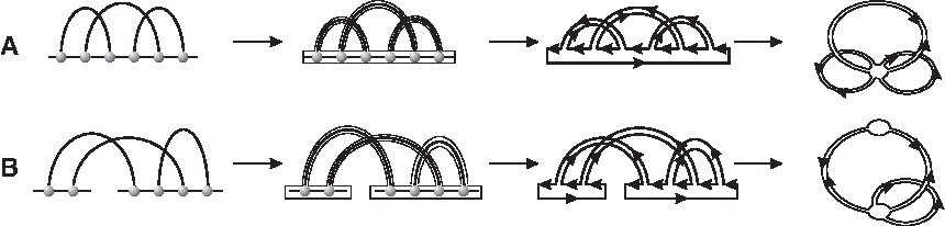
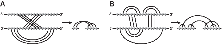
We strongly suspect that such complex interactions are common among the many thousands of long noncoding RNAs, which in the last years have been discovered as important regulatory molecules. It is crucial, therefore, to better understand the theoretical possibilities and to systematically investigate how more complex classes of interaction structure can be addressed algorithmically. In Figure 15, we show that 0-interaction structures are different from AP-structures (Pervouchine, 2004; Alkan et al., 2006).

FIG. 15.
(A) A 0-interaction structure over two backbones that is not an AP-structure; the crossing hybrid. (B) An AP-structure that is not a 0-structure over two backbones; this structure contains an irreducible shadow over two backbones of genus 1.

Let us come back to the recursive constructions that result from algebraic-generating functions. We argued above that the derivation of bivariate algebraic equations as Equation (3.2) is crucial for obtaining recursions for computing shadows of genus g from those of smaller genera. Similar to the Zagier-Harer generating function (Zagier, 1995), the derivation of recursions for the polynomials I_g,2(z) is now work in progress (Fu, 2012). Common factors of these polynomials whose coefficients count numbers of irreducible shadows of fixed genus will be the key for deeper understanding. Accordingly, it is of importance to compute the polynomials I_g,2(z) explicitly for all relevant genera.

Furthermore, this line of work has led to a bijection between genus zero interaction structures and certain pairs of plane trees with some distinguished vertices (Han, 2012). This bijection is new and its algorithmic implications are certainly not fully understood. However, we expect profound impact and novel insights on how to fold interaction structures faster. One immediate implication concerns the parallelization of the interaction structure folding.

In this article, we offer a general mathematical foundation for the nucleic acid interaction problem. This framework is instrumental for devising algorithms for RNA–RNA interaction structures that employ the combinatorial/topological structure of the classification of interaction structures.

6. Appendix

A-1: Proof of Theorem 1

Proof. First, we begin by claiming an observation about shadows over one backbone from Reidys et al. (2011) as follows.

Shadows of genus g ≥ 1 over one backbone have the following properties:

(a) a shadow of genus g contains at least 2g and at most (6g − 2) arcs; in particular for fixed genus, there are only finitely many shadows;

(b) for any 2g ≤ ℓ ≤ 6g − 2, there exists a shadow of genus g containing exactly ℓ arcs.

To prove this claim, first note that if there is more than one boundary component, then there must be an arc with different boundary components on its two sides, and removing this arc decreases r by exactly one while preserving g since the number of arcs is given by n = 2g + r − 1. Furthermore, if there are ν_ℓ boundary components of length ℓ in the polygonal model, then 2n = ∑_ℓℓν_ℓ since each side of each arc is traversed once by the boundary. For a shadow, ν₁ = 0 by definition, and ν₂ ≤ 1 as one sees directly. It therefore follows that 2n = ∑_ℓℓν_ℓ ≥ 3(r − 1) + 2, so 2n = 4g + 2r − 2 ≥ 3r − 1, i.e., 4g − 1 ≥ r. Thus, we have n = 2g + (4g − 1) − 1 = 6g − 2, that is, any shadow can contain at most 6g − 2 arcs. The lower bound 2g follows directly from n = 2g + r − 1 since r ≥ 1.

Let S_2g be a shadow containing 2g mutually crossing arcs, that is, each arc crosses any of the remaining (2g − 1) arcs. S_2g has genus g and contains a unique boundary component of length 4g, that is, traversing 4g nonbackbone arcs counted with multiplicity. We construct a new shadow S_2g+1 of genus g containing 2g + 1 arcs by inserting an arc crossing into S_2g from the 5′ end of S_2g such that the boundary component in S_2g splits into one boundary component of length 3 and another of length 4g + 2 − 3 = 4g − 1. The latter becomes the first boundary component of S_2g+1. The newly inserted arc is, by construction, crossing, splitting a boundary component, and preserving genus. We now prove the assertion by induction of the number of inserted arcs. By the induction hypothesis, there exists a shadow S_2g+i of genus g having 2g + i arcs, whose first boundary component has length 4g − i. Again, we insert a crossing arc as described above, thereby splitting the first boundary component into one of length 3 and the other of length (4g − (i + 1)). After i = 4g − 2 such insertions, we arrive at a shadow whose first boundary component has length 2 while all other boundary components have length 3. Accordingly, there exists a set \documentclass{aastex}\usepackage{amsbsy}\usepackage{amsfonts}\usepackage{amssymb}\usepackage{bm}\usepackage{mathrsfs}\usepackage{pifont}\usepackage{stmaryrd}\usepackage{textcomp}\usepackage{portland, xspace}\usepackage{amsmath, amsxtra}\pagestyle{empty}\DeclareMathSizes{10}{9}{7}{6}\begin{document}$$\{S_{2g} , S_{2g + 1} , \ldots , S_{2g + ( 4g - 2 )} \} $$\end{document} of shadows all having genus g, where each S_j contains j arcs.

We next claim that any shadow of genus g over two backbones can be obtained by cutting the backbone of a shadow over one backbone having either genus g or g + 1. To see this, suppose we are given a shadow of genus g, having r boundary components and n arcs so that 2 − 2g − r = b − n, that is, g = (2 + n − r −b)/2, where b = 1. Cutting the backbone then either splits a boundary component or merges two distinct boundary components. Since cutting does not affect arcs and increases the number of backbones by one, we have the resulting genus \documentclass{aastex}\usepackage{amsbsy}\usepackage{amsfonts}\usepackage{amssymb}\usepackage{bm}\usepackage{mathrsfs}\usepackage{pifont}\usepackage{stmaryrd}\usepackage{textcomp}\usepackage{portland, xspace}\usepackage{amsmath, amsxtra}\pagestyle{empty}\DeclareMathSizes{10}{9}{7}{6}\begin{document}\begin{align}g^{\prime} = ( 2 + n - ( r + 1 ) - ( b + 1 ) ) / 2 = g - 1 \quad {\rm or} \quad g^{\prime} = ( 2 + n - ( r - 1 ) - ( b + 1 ) ) / 2 = g\end{align}\end{document}

as was claimed. We next observe that a shadow of genus g = 0 over two backbones has at least two arcs, while the maximum number of arcs contained in such a shadow is given by 6(0 + 1) − 2 = 4. For g ≥ 1, it is impossible to cut a shadow of genus g having 2g arcs and keep the genus. Thus, the shadow of genus g over two backbones has at least 2g + 1 arcs. We can always map an arbitrary shadow over two backbones of genus g via α into a shadow over one backbone, whence the assertion. The first claim guarantees that there are only finitely many such shadows, and the theorem follows. ■

A-2: Proof of Corollary 1

Proof. Part (a) follows directly from the first claim in A-1, and for (b), the shadows \documentclass{aastex}\usepackage{amsbsy}\usepackage{amsfonts}\usepackage{amssymb}\usepackage{bm}\usepackage{mathrsfs}\usepackage{pifont}\usepackage{stmaryrd}\usepackage{textcomp}\usepackage{portland, xspace}\usepackage{amsmath, amsxtra}\pagestyle{empty}\DeclareMathSizes{10}{9}{7}{6}\begin{document}$$S_{2g + 1} , \ldots , S_{6g - 2}$$\end{document} generated in the proof of the first claim in A-1 are, in fact, irreducible. ■

n	n = 1	n = 2	n = 3	n = 4	n = 5	n = 6	n = 7	n = 8
q₀(n)	1	8	54	340	2062	12242	71795	418078

Footnotes

Author Disclosure Statement

No competing financial interests exist.

References

Alkan

, Karakoc

, Nadeau

J.H.

et al. 2006. RNA-RNA interaction prediction and antisense RNA target search. J. Comput. Biol., 13:267–282.

Andersen

J.E.

, Huang

F.W.D.

, Penner

R.C.

, Reidys

C.M.

2012. Topology of RNA-RNA interaction structures. J. Comp. Biol., 19:928–943.

Bernhart

, Tafer

, Mückstein

et al. 2006. Partition function and base pairing probabilities of RNA heterodimers. Algorithms Mol. Biol., 1:3.

Bon

, Vernizzi

, Orland

, Zee

2008. Topological classification of RNA structures. J. Mol. Biol., 379:900–911.

Busch

, Richter

A.S.

, Backofen

2008. IntraRNA: efficient prediction of bacterial sRNA targets incorporating target site accessibility and seed regions. Bioinformatics, 24:2849–2856.

Flajolet

, Sedgewick

2009. Analytic Combinatorics. Cambridge University Press: New York.

B.M.M.

2012. Personal communication.

Han

H.S.W.

2012. Personal communication.

Han

H.S.W.

, Li

T.J.X.

, Reidys

C.M.

2012. Combinatorics of γ-structures. submitted, arXiv:1112.4151v1.

10.

Hofacker

I.L.

, Fontana

, Stadler

P.F.

et al. 1994. Fast folding and comparison of RNA secondary structures. Monatsh. Chem., 125:167–188.

11.

Huang

F.W.D.

, Qin

, Reidys

C.M.

, Stadler

P.F.

2009. Partition function and base pairing probabilities for RNA-RNA interaction prediction. Bioinformatics, 25:2646–2654.

12.

Huang

F.W.D.

, Qin

, Reidys

C.M.

, Stadler

P.F.

2010. Target prediction and a statistical sampling algorithm for RNA-RNA interaction. Bioinformatics, 26:175–181.

13.

Kiss

A.M.

, Jady

B.E.

, Bertrand

, Kiss

2004. Human box H/ACA pseudouridylation guide RNA machinery. Mol. Cell. Biol., 24:5797–5807.

14.

, Xu

, Rivera

M.A.

et al. 2003. A role for a novel ‘trans-pseudoknot’ RNA-RNA interaction in the functional dimerization of human telomerase. Genes & Dev., 17:1078–1083.

15.

Massey

W.S.

1967. Algebraic Topology: An Introduction. Springer-Veriag: New York.

16.

Mückstein

, Tafer

, Bernhard

S.H.

et al. 2008. Translational control by RNA-RNA interaction: Improved computation of RNA-RNA binding thermodynamics. 114–127

Elloumi

, Küng

, Linial

et al. BioInformatics Research and Development—BIRD 2008, 13. Springer: Berlin.

17.

Mückstein

, Tafer

, Hackermüller

et al. 2006. Thermodynamics of RNA-RNA binding. Bioinformatics, 22:1177–1182.

18.

Ofengand

, Bakin

1997. Mapping to nucleotide resolution of pseudouridine residues in large subunit ribosomal RNAs from representative eukaryotes, prokaryotes, archaebacteria, mitochondria and chloroplasts. J. Mol. Biol., 266:246–268.

19.

Orland

, Zee

2002. RNA folding and large n matrix theory. Nuclear Physics B, 620:456–476.

20.

Penner

R.C.

2004. Cell decomposition and compactification of Riemann's moduli space in decorated Teichmüller theory. 263–301

Tongring

, Penner

R.C.

Woods Hole Mathematics-Perspectives in Math and Physics. World Scientific: Singapore.

21.

Penner

R.C.

2011. Decorated Teichmüller Theory. European Mathematical Society: Zürich.

22.

Penner

R.C.

, Waterman

M.S.

1993. Spaces of RNA secondary structures. Adv. Math., 101:31–49.

23.

Penner

R.C.

, Knudsen

, Wiuf

, Andersen

2010. Fatgraph models of proteins. Comm. Pure Appl. Math., 63:1249–1297.

24.

Pervouchine

D. D.

2004. IRIS: Intermolecular RNA interaction search. Proc. Genome Informatics, 15:92–101.

25.

Reidys

C.M.

, Huang

F.W.D.

, Andersen

J.E.

et al. 2011. Topology and prediction of RNA pseudoknots. Bioinformatics, 27:1076–1085.

26.

Rivas

, Eddy

S.R.

1999. A dynamic programming algorithms for RNA structure prediction including pseudoknots. J. Mol. Biol., 285:2053–2068.

27.

Vernizzi

, Orland

2005. Large-N random matrices for RNA folding. Acta Phys. Polon., 36:2821–2827.

28.

Zagier

1995. On the distribution of the number of cycles of elements in symmetric groups. Nieuw Arch. Wisk. IV, 13:489–495.