The problem of finding the locations in DNA sequences that match a given motif describing the binding specificities of a transcription factor (TF) has many applications in computational biology. This problem has been extensively studied when the position weight matrix (PWM) model is used to represent motifs. We investigate it under the feature motif model, a generalization of the PWM model that does not assume independence between positions in the pattern while being compatible with the original PWM. We present a new method for finding the binding sites of a transcription factor in a DNA sequence when the feature motif model is used to describe transcription factor binding specificities. The experimental results on random and real data show that the search algorithm is fast in practice.
1. Introduction
The binding of transcription factor proteins to their target DNA sequences is a fundamental process in the transcription of genetic information. Two main computational problems that arise from the study of these interactions are: i) finding an accurate model to describe the binding specificities of a given transcription factor; and ii) given a DNA sequence and a motif that describes the binding specificities of a given transcription factor, finding all the binding sites in the sequence that match the motif. The traditional model used to represent transcription factor motifs is the position weight matrix (PWM) (Stormo et al., 1982; Schneider et al., 1986; Gribskov et al., 1987). In this model, a motif of length m is represented using a matrix of size m × |Σ|, where Σ is an alphabet of size 4 (DNA) in this context; each cell of the matrix contains the position-specific weights for each symbol in the alphabet, that is, the cell mij contains the weight contributed by an occurrence of the j-th symbol at the i-th position. This model assumes that there is no correlation between positions in the sites, that is, the contribution of a nucleotide at a given position to the total affinity does not depend on the other nucleotides that appear in other positions. The problem of matching the locations in DNA sequences at which a given transcription factor protein binds to is well studied under the PWM model (Pizzi and Ukkonen, 2008). One application where this problem becomes relevant is, for example, described in Hallikas et al. (2006).
Many more advanced models have been proposed to overcome the independence assumption of the PWM; among them are the maximal dependence decomposition (MDD) (Burge and Karlin, 1997), the generalized weight matrix (GWM) (Zhou and Liu, 2004), the permuted variable length Markov models (PVLMM) (Zhao et al., 2005), feature motif model (FMM) (Sharon et al., 2008), the dinucleotide weight matrix (DWM) (Siddharthan, 2010), and the tree-based position weight matrix (TPWM) (Bi et al., 2011). While some of these models are not compatible with the original PWM representation, others are actually a generalized version of it. In this article, we deal with this latter type of model as we believe that they have a greater chance to replace the standard PWM model. In particular, we focus on the FMM (Sharon et al., 2008) since, to our knowledge, it is the most general one. However, our approach can also be applied, with small changes, to other similar models.
In the FMM model, the TF-binding specificities are described with so-called features, that is, rules that assign a weight to a set of associations between symbols and positions. In particular, a PWM can be expressed as a set of features that include a single association; in this respect, it is a special case of this more general model. Given a DNA sequence, a set of features and a motif length m, the matching problem consists of computing the score of each site (substring) of length m in the sequence, where the score of a site is the sum of the weights of all the features that occur in the site.
To our knowledge, the problem of matching transcription-factor motifs using the FMM model has not been investigated yet. In this work, we present a fast method to match FMM motifs. Our method is based on a reduction of this problem to the one of matching a set of gapped q-gram patterns in a given sequence, where a q-gram pattern is a sequence of q symbols, over a finite alphabet Σ, such that there is a gap of fixed length between each two consecutive symbols. In particular, we are interested in computing the list of matching patterns for each position in the sequence. This problem is a specific instance of the variable length gaps problem (VLG problem) for multiple patterns. Note that, although the number of associations in a feature in the FMM model can be up to m, the experimental evaluation presented in Sharon et al. (2008) allows for up to two associations. In this work, we focus on the case of two associations only, that is, the features are 2 grams with a fixed-length gap between the two symbols.
We then present a framework for the problem of matching FMM motifs that uses such an algorithm as a component and describes novel simple algorithms for the problem of matching a set of gapped q-gram patterns in the q = 2 case. The proposed algorithms are fast when the gap lengths in the patterns are constrained, which is a reasonable assumption in this context since the motifs are usually short. Our method is considerably faster than a naive search of all the features for each site in the sequence.
The rest of the article is organized as follows. In Section 2, we recall some preliminary notions and elementary facts. In Section 3, we present our method to find transcription-factor motifs using the FMM model. In Section 4, we present new algorithms for the problem of matching gapped q-gram patterns, which we use as a component in our method. In Section 5, we present experimental results on random and real data of our new algorithms and of the full method. Finally, we briefly discuss our conclusions in Section 6.
2. Basic Notions And Definitions
Let \documentclass{aastex}\usepackage{amsbsy}\usepackage{amsfonts}\usepackage{amssymb}\usepackage{bm}\usepackage{mathrsfs}\usepackage{pifont}\usepackage{stmaryrd}\usepackage{textcomp}\usepackage{portland, xspace}\usepackage{amsmath, amsxtra}\pagestyle{empty}\DeclareMathSizes{10}{9}{7}{6}\begin{document}
$$\Sigma = \{ c_1 , c_2 , \ldots , c_{ \sigma} \} $$
\end{document} denote an alphabet of size σ. Let Σ* denote the Kleene star of Σ, and Σm the set of all possible sequences of length m over Σ. |S| is the length of string S, S[i], i ≥ 0, denotes its (i + 1)-th character, and \documentclass{aastex}\usepackage{amsbsy}\usepackage{amsfonts}\usepackage{amssymb}\usepackage{bm}\usepackage{mathrsfs}\usepackage{pifont}\usepackage{stmaryrd}\usepackage{textcomp}\usepackage{portland, xspace}\usepackage{amsmath, amsxtra}\pagestyle{empty}\DeclareMathSizes{10}{9}{7}{6}\begin{document}
$$S [ i , \ldots \, , j ]$$
\end{document} its substring between the (i + 1)-st and the (j + 1)-st characters (inclusive). A gapped q-gram pattern is of the form
\documentclass{aastex}\usepackage{amsbsy}\usepackage{amsfonts}\usepackage{amssymb}\usepackage{bm}\usepackage{mathrsfs}\usepackage{pifont}\usepackage{stmaryrd}\usepackage{textcomp}\usepackage{portland, xspace}\usepackage{amsmath, amsxtra}\pagestyle{empty}\DeclareMathSizes{10}{9}{7}{6}\begin{document}\begin{align*}( \,p_1 \cdot j_1 \cdot p_2 \cdot \ldots \cdot j_{q- 1} \cdot p_q )\end{align*}\end{document}
where \documentclass{aastex}\usepackage{amsbsy}\usepackage{amsfonts}\usepackage{amssymb}\usepackage{bm}\usepackage{mathrsfs}\usepackage{pifont}\usepackage{stmaryrd}\usepackage{textcomp}\usepackage{portland, xspace}\usepackage{amsmath, amsxtra}\pagestyle{empty}\DeclareMathSizes{10}{9}{7}{6}\begin{document}$$\langle \,p_1 , p_2 , \ldots , p_q \rangle$$\end{document} is a sequence of q symbols and \documentclass{aastex}\usepackage{amsbsy}\usepackage{amsfonts}\usepackage{amssymb}\usepackage{bm}\usepackage{mathrsfs}\usepackage{pifont}\usepackage{stmaryrd}\usepackage{textcomp}\usepackage{portland, xspace}\usepackage{amsmath, amsxtra}\pagestyle{empty}\DeclareMathSizes{10}{9}{7}{6}\begin{document}$$\langle \,j_1 , j_2 , \ldots , j_{q - 1} \rangle$$\end{document} is the associated sequence of gaps, that is, jk\documentclass{aastex}\usepackage{amsbsy}\usepackage{amsfonts}\usepackage{amssymb}\usepackage{bm}\usepackage{mathrsfs}\usepackage{pifont}\usepackage{stmaryrd}\usepackage{textcomp}\usepackage{portland, xspace}\usepackage{amsmath, amsxtra}\pagestyle{empty}\DeclareMathSizes{10}{9}{7}{6}\begin{document}$$\in$$\end{document}N is the length of the gap between symbols pk and pk+1. We say that a gapped q-gram pattern \documentclass{aastex}\usepackage{amsbsy}\usepackage{amsfonts}\usepackage{amssymb}\usepackage{bm}\usepackage{mathrsfs}\usepackage{pifont}\usepackage{stmaryrd}\usepackage{textcomp}\usepackage{portland, xspace}\usepackage{amsmath, amsxtra}\pagestyle{empty}\DeclareMathSizes{10}{9}{7}{6}\begin{document}$$( p_1 \cdot j_1 \cdot p_2 \cdot \ldots \cdot j_{q - 1} \cdot p_q )$$\end{document} occurs in S at ending position i if
\documentclass{aastex}\usepackage{amsbsy}\usepackage{amsfonts}\usepackage{amssymb}\usepackage{bm}\usepackage{mathrsfs}\usepackage{pifont}\usepackage{stmaryrd}\usepackage{textcomp}\usepackage{portland, xspace}\usepackage{amsmath, amsxtra}\pagestyle{empty}\DeclareMathSizes{10}{9}{7}{6}\begin{document}
\begin{align*}S [ i - \sum_{i = k}^{q - 1} ( \, j_i + 1 ) ] = p_k ,\end{align*}
\end{document}
for \documentclass{aastex}\usepackage{amsbsy}\usepackage{amsfonts}\usepackage{amssymb}\usepackage{bm}\usepackage{mathrsfs}\usepackage{pifont}\usepackage{stmaryrd}\usepackage{textcomp}\usepackage{portland, xspace}\usepackage{amsmath, amsxtra}\pagestyle{empty}\DeclareMathSizes{10}{9}{7}{6}\begin{document}$$k = 1 , \ldots , q$$\end{document}. Given a set \documentclass{aastex}\usepackage{amsbsy}\usepackage{amsfonts}\usepackage{amssymb}\usepackage{bm}\usepackage{mathrsfs}\usepackage{pifont}\usepackage{stmaryrd}\usepackage{textcomp}\usepackage{portland, xspace}\usepackage{amsmath, amsxtra}\pagestyle{empty}\DeclareMathSizes{10}{9}{7}{6}\begin{document}
$${ \cal P}$$
\end{document} of gapped q-gram patterns, we denote with gspan (\documentclass{aastex}\usepackage{amsbsy}\usepackage{amsfonts}\usepackage{amssymb}\usepackage{bm}\usepackage{mathrsfs}\usepackage{pifont}\usepackage{stmaryrd}\usepackage{textcomp}\usepackage{portland, xspace}\usepackage{amsmath, amsxtra}\pagestyle{empty}\DeclareMathSizes{10}{9}{7}{6}\begin{document}$${ \cal P}$$\end{document}) the number of distinct gap lengths in \documentclass{aastex}\usepackage{amsbsy}\usepackage{amsfonts}\usepackage{amssymb}\usepackage{bm}\usepackage{mathrsfs}\usepackage{pifont}\usepackage{stmaryrd}\usepackage{textcomp}\usepackage{portland, xspace}\usepackage{amsmath, amsxtra}\pagestyle{empty}\DeclareMathSizes{10}{9}{7}{6}\begin{document}$${ \cal P}$$\end{document}.
The RAM model is assumed, with machine word size w = Ω(log n). We use some bitwise operations following the standard notation as in C language: &, |, ∼, ≪ for and, or, not, and left shift, respectively. The function to compute the position of the most significant set bit of a word x is ⌊log2(x)⌋.
3. Method
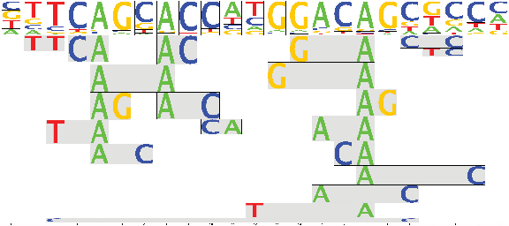
The FMM (Sharon et al., 2008) is a relatively new model to represent the interactions between transcription factors and their target DNA sequences. In the FMM model, the TF-binding specificities are described with so-called features, that is, rules that assign a weight to a set of associations between symbols and positions. Given a DNA sequence T, a set of features and a motif length m, the matching problem consists in computing the score of each site (substring) of length m in the sequence T, where the score of a site is the sum of the weights of all the features that occur in the site. Figure 1, taken from the Segal Lab website, shows an example of FMM motif, visualized as a sequence logo. The motif is of length 23 and consists of 20 2-gram features and 4 × 23 1-gram features. The 1-gram features taken together represent a PWM. The height of each letter gives the weight of the corresponding feature.
Feature motif model (FMM) of the neuron-restrictive silencer factor (NRSF) protein.
Formally, a feature can be denoted as
\documentclass{aastex}\usepackage{amsbsy}\usepackage{amsfonts}\usepackage{amssymb}\usepackage{bm}\usepackage{mathrsfs}\usepackage{pifont}\usepackage{stmaryrd}\usepackage{textcomp}\usepackage{portland, xspace}\usepackage{amsmath, amsxtra}\pagestyle{empty}\DeclareMathSizes{10}{9}{7}{6}\begin{document}\begin{align*}\{ ( a_1 , i_1 ) , \ldots , ( a_q , i_q ) \} \rightarrow w\end{align*}\end{document}
where w is the affinity contribution of the feature and \documentclass{aastex}\usepackage{amsbsy}\usepackage{amsfonts}\usepackage{amssymb}\usepackage{bm}\usepackage{mathrsfs}\usepackage{pifont}\usepackage{stmaryrd}\usepackage{textcomp}\usepackage{portland, xspace}\usepackage{amsmath, amsxtra}\pagestyle{empty}\DeclareMathSizes{10}{9}{7}{6}\begin{document}$$a_j \in \{ A , C , G , T \} $$\end{document} is the nucleotide that must occur at position ij, for \documentclass{aastex}\usepackage{amsbsy}\usepackage{amsfonts}\usepackage{amssymb}\usepackage{bm}\usepackage{mathrsfs}\usepackage{pifont}\usepackage{stmaryrd}\usepackage{textcomp}\usepackage{portland, xspace}\usepackage{amsmath, amsxtra}\pagestyle{empty}\DeclareMathSizes{10}{9}{7}{6}\begin{document}$$j = 1 , \ldots , q$$\end{document} and 1 ≤ ij ≤ m. It is easy to transform these rules into new rules where the left side is a gapped q-gram pattern: if \documentclass{aastex}\usepackage{amsbsy}\usepackage{amsfonts}\usepackage{amssymb}\usepackage{bm}\usepackage{mathrsfs}\usepackage{pifont}\usepackage{stmaryrd}\usepackage{textcomp}\usepackage{portland, xspace}\usepackage{amsmath, amsxtra}\pagestyle{empty}\DeclareMathSizes{10}{9}{7}{6}\begin{document}$$i_1 < i_2 < \ldots < i_q$$\end{document}, we can induce the following gapped q-gram pattern rule
\documentclass{aastex}\usepackage{amsbsy}\usepackage{amsfonts}\usepackage{amssymb}\usepackage{bm}\usepackage{mathrsfs}\usepackage{pifont}\usepackage{stmaryrd}\usepackage{textcomp}\usepackage{portland, xspace}\usepackage{amsmath, amsxtra}\pagestyle{empty}\DeclareMathSizes{10}{9}{7}{6}\begin{document}
\begin{align*}( a_1 \cdot ( i_2 - i_1 - 1 ) \cdot \ldots \cdot (i_q , i_{q - 1} - 1 ) \cdot a_q ) \rightarrow ( i_q , w).\end{align*}\end{document}
This transformation has the advantage that the resulting pattern is position independent. Moreover, after this transformation, different features may share the same gapped q-gram pattern. For example, the features {(a, 1), (c, 3)} and {(a, 3), (c, 5)} map onto the same pattern {a·2·c}. Then, the matching problem can be decomposed into two components: the first component identifies the occurrences of the groups of features by searching for the corresponding gapped q-gram patterns while the second component computes the score for each candidate site using the information provided by the first component.
For a motif of length m, the second component can be easily implemented by maintaining the score for m sites simultaneously with a circular queue of length m. Each time a group of features with an associated set of position/weight pairs \documentclass{aastex}\usepackage{amsbsy}\usepackage{amsfonts}\usepackage{amssymb}\usepackage{bm}\usepackage{mathrsfs}\usepackage{pifont}\usepackage{stmaryrd}\usepackage{textcomp}\usepackage{portland, xspace}\usepackage{amsmath, amsxtra}\pagestyle{empty}\DeclareMathSizes{10}{9}{7}{6}\begin{document}$$\{ ( i_1 , w_1 ) , \ldots , ( i_r , w_r ) \} $$\end{document} is found at position j in the sequence, the algorithm adds the weight wk to the score of the alignment that ends at position j + m − ik in the sequence, if j ≥ ik.
4. Algorithms
In this section, we present two simple algorithms to search for the occurrences of a set \documentclass{aastex}\usepackage{amsbsy}\usepackage{amsfonts}\usepackage{amssymb}\usepackage{bm}\usepackage{mathrsfs}\usepackage{pifont}\usepackage{stmaryrd}\usepackage{textcomp}\usepackage{portland, xspace}\usepackage{amsmath, amsxtra}\pagestyle{empty}\DeclareMathSizes{10}{9}{7}{6}\begin{document}$${ \cal P}$$\end{document} of gapped 2-gram patterns in a text T of length n, defined over a finite alphabet Σ of size σ. This problem is a specific instance of the VLG problem for multiple patterns. In the VLG problem, a pattern is a concatenation of strings and of variable length gaps. In the specific scenario of gapped q-gram patterns, where all the strings in the patterns have unitary length, the available more general algorithms for this problem do not scale well in the case of multiple patterns. In particular, to our knowledge, the best practical methods for the VLG problem are those introduced in Bille et al. (2010) and Haapasalo et al. (2011). In our problem, the first algorithm has O(n + α)-time complexity, where α is the number of occurrences of the pattern strings (key words) in the text T. Note that the number of occurrences of a key word that occurs in r patterns and in l positions in the text is equal to r × l. Instead, the second algorithm has O(n + α′)-time complexity, where α′ is the number of occurrences in the text of pattern prefixes ending with a key word. In the case of multiple patterns, these results are not ideal because, if we assume a uniform distribution for the patterns, we have on average that α and α′ are \documentclass{aastex}\usepackage{amsbsy}\usepackage{amsfonts}\usepackage{amssymb}\usepackage{bm}\usepackage{mathrsfs}\usepackage{pifont}\usepackage{stmaryrd}\usepackage{textcomp}\usepackage{portland, xspace}\usepackage{amsmath, amsxtra}\pagestyle{empty}\DeclareMathSizes{10}{9}{7}{6}\begin{document}$$\Omega ( n \frac { len ( { \cal P ) } } { \sigma } )$$\end{document} and \documentclass{aastex}\usepackage{amsbsy}\usepackage{amsfonts}\usepackage{amssymb}\usepackage{bm}\usepackage{mathrsfs}\usepackage{pifont}\usepackage{stmaryrd}\usepackage{textcomp}\usepackage{portland, xspace}\usepackage{amsmath, amsxtra}\pagestyle{empty}\DeclareMathSizes{10}{9}{7}{6}\begin{document}
$$\Omega ( n \frac { \mid { \cal P } \mid } { \sigma } )$$
\end{document}, respectively, where len(\documentclass{aastex}\usepackage{amsbsy}\usepackage{amsfonts}\usepackage{amssymb}\usepackage{bm}\usepackage{mathrsfs}\usepackage{pifont}\usepackage{stmaryrd}\usepackage{textcomp}\usepackage{portland, xspace}\usepackage{amsmath, amsxtra}\pagestyle{empty}\DeclareMathSizes{10}{9}{7}{6}\begin{document}
$${ \cal P}$$
\end{document}) is the sum of the number of symbols in each pattern.
Our first algorithm for q = 2, based on the “Four Russians” technique (Arlazarov et al., 1970), has O(n + ngspan(\documentclass{aastex}\usepackage{amsbsy}\usepackage{amsfonts}\usepackage{amssymb}\usepackage{bm}\usepackage{mathrsfs}\usepackage{pifont}\usepackage{stmaryrd}\usepackage{textcomp}\usepackage{portland, xspace}\usepackage{amsmath, amsxtra}\pagestyle{empty}\DeclareMathSizes{10}{9}{7}{6}\begin{document}
$${ \cal P}$$
\end{document})/h + occ)-time complexity, where gspan(\documentclass{aastex}\usepackage{amsbsy}\usepackage{amsfonts}\usepackage{amssymb}\usepackage{bm}\usepackage{mathrsfs}\usepackage{pifont}\usepackage{stmaryrd}\usepackage{textcomp}\usepackage{portland, xspace}\usepackage{amsmath, amsxtra}\pagestyle{empty}\DeclareMathSizes{10}{9}{7}{6}\begin{document}
$${ \cal P}$$
\end{document}) is the number of distinct gap lengths in \documentclass{aastex}\usepackage{amsbsy}\usepackage{amsfonts}\usepackage{amssymb}\usepackage{bm}\usepackage{mathrsfs}\usepackage{pifont}\usepackage{stmaryrd}\usepackage{textcomp}\usepackage{portland, xspace}\usepackage{amsmath, amsxtra}\pagestyle{empty}\DeclareMathSizes{10}{9}{7}{6}\begin{document}
$${ \cal P}$$
\end{document}, and h is a parameter. The second algorithm, based on bit-parallelism (Baeza-Yates and Gonnet, 1992), has O(n⌈ℓ/w ⌉ + occ)-time complexity, where gsize(\documentclass{aastex}\usepackage{amsbsy}\usepackage{amsfonts}\usepackage{amssymb}\usepackage{bm}\usepackage{mathrsfs}\usepackage{pifont}\usepackage{stmaryrd}\usepackage{textcomp}\usepackage{portland, xspace}\usepackage{amsmath, amsxtra}\pagestyle{empty}\DeclareMathSizes{10}{9}{7}{6}\begin{document}
$${ \cal P}$$
\end{document}) ≤ ℓ ≤ σgsize (\documentclass{aastex}\usepackage{amsbsy}\usepackage{amsfonts}\usepackage{amssymb}\usepackage{bm}\usepackage{mathrsfs}\usepackage{pifont}\usepackage{stmaryrd}\usepackage{textcomp}\usepackage{portland, xspace}\usepackage{amsmath, amsxtra}\pagestyle{empty}\DeclareMathSizes{10}{9}{7}{6}\begin{document}
$${ \cal P}$$
\end{document}) and gsize(\documentclass{aastex}\usepackage{amsbsy}\usepackage{amsfonts}\usepackage{amssymb}\usepackage{bm}\usepackage{mathrsfs}\usepackage{pifont}\usepackage{stmaryrd}\usepackage{textcomp}\usepackage{portland, xspace}\usepackage{amsmath, amsxtra}\pagestyle{empty}\DeclareMathSizes{10}{9}{7}{6}\begin{document}
$${ \cal P}$$
\end{document}) is the size of the variation range of the gap lengths in \documentclass{aastex}\usepackage{amsbsy}\usepackage{amsfonts}\usepackage{amssymb}\usepackage{bm}\usepackage{mathrsfs}\usepackage{pifont}\usepackage{stmaryrd}\usepackage{textcomp}\usepackage{portland, xspace}\usepackage{amsmath, amsxtra}\pagestyle{empty}\DeclareMathSizes{10}{9}{7}{6}\begin{document}
$${ \cal P}$$
\end{document}. The second algorithm is good when σ and gsize(\documentclass{aastex}\usepackage{amsbsy}\usepackage{amsfonts}\usepackage{amssymb}\usepackage{bm}\usepackage{mathrsfs}\usepackage{pifont}\usepackage{stmaryrd}\usepackage{textcomp}\usepackage{portland, xspace}\usepackage{amsmath, amsxtra}\pagestyle{empty}\DeclareMathSizes{10}{9}{7}{6}\begin{document}
$${ \cal P}$$
\end{document}) are small. Otherwise, the first algorithm is preferable.
We assume that all the patterns in \documentclass{aastex}\usepackage{amsbsy}\usepackage{amsfonts}\usepackage{amssymb}\usepackage{bm}\usepackage{mathrsfs}\usepackage{pifont}\usepackage{stmaryrd}\usepackage{textcomp}\usepackage{portland, xspace}\usepackage{amsmath, amsxtra}\pagestyle{empty}\DeclareMathSizes{10}{9}{7}{6}\begin{document}
$${ \cal P}$$
\end{document} are distinct, that is, for any \documentclass{aastex}\usepackage{amsbsy}\usepackage{amsfonts}\usepackage{amssymb}\usepackage{bm}\usepackage{mathrsfs}\usepackage{pifont}\usepackage{stmaryrd}\usepackage{textcomp}\usepackage{portland, xspace}\usepackage{amsmath, amsxtra}\pagestyle{empty}\DeclareMathSizes{10}{9}{7}{6}\begin{document}
$$c_1 , c_2 \in \Sigma$$
\end{document}, and \documentclass{aastex}\usepackage{amsbsy}\usepackage{amsfonts}\usepackage{amssymb}\usepackage{bm}\usepackage{mathrsfs}\usepackage{pifont}\usepackage{stmaryrd}\usepackage{textcomp}\usepackage{portland, xspace}\usepackage{amsmath, amsxtra}\pagestyle{empty}\DeclareMathSizes{10}{9}{7}{6}\begin{document}
$$j \in N$$
\end{document}, there exists at most one i such that ai = c1, bi = c2, and ji = j. Let G be the set of all the distinct gap lengths in the patterns. For each \documentclass{aastex}\usepackage{amsbsy}\usepackage{amsfonts}\usepackage{amssymb}\usepackage{bm}\usepackage{mathrsfs}\usepackage{pifont}\usepackage{stmaryrd}\usepackage{textcomp}\usepackage{portland, xspace}\usepackage{amsmath, amsxtra}\pagestyle{empty}\DeclareMathSizes{10}{9}{7}{6}\begin{document}
$$j \in G$$
\end{document}, we maintain a lookup table (LUT) Lj of size σ2h, where 1 ≤ h ≤ ⌊log n/log σ⌋ is a parameter. For any two strings S1 and S2 of length h, we have that Lj (S1, S2) contains the list of all the pairs (i, k) such that
\documentclass{aastex}\usepackage{amsbsy}\usepackage{amsfonts}\usepackage{amssymb}\usepackage{bm}\usepackage{mathrsfs}\usepackage{pifont}\usepackage{stmaryrd}\usepackage{textcomp}\usepackage{portland, xspace}\usepackage{amsmath, amsxtra}\pagestyle{empty}\DeclareMathSizes{10}{9}{7}{6}\begin{document}
\begin{align*}S_1 [ k ] = a_i \wedge S_2 [ k ] = b_i \wedge j = j_i\end{align*}
\end{document}
for 1 ≤ i ≤ l and 0 ≤ k < h. For h = 1, the LUT definition can be simplified to
\documentclass{aastex}\usepackage{amsbsy}\usepackage{amsfonts}\usepackage{amssymb}\usepackage{bm}\usepackage{mathrsfs}\usepackage{pifont}\usepackage{stmaryrd}\usepackage{textcomp}\usepackage{portland, xspace}\usepackage{amsmath, amsxtra}\pagestyle{empty}\DeclareMathSizes{10}{9}{7}{6}\begin{document}
\begin{align*}L_j ( c_1 , c_2 ) = \begin{cases} {i \qquad { \rm if } \ c_1 = a_i \wedge c_2 = b_i \wedge j = j_i} \\ {0 \qquad { \rm otherwise}}\end{cases}\end{align*}
\end{document}
The first algorithm, named gq1, works as follows: first, T is packed to T′, so that each symbol occupies only ⌈log σ⌉ bits. This phase is performed in O(n) time. For h = 1 it is possible to skip this pass and set T′ = T. Let Ti = T[i − h + 1.i] be the substring of T of length h ending at position i. The packed encoding of any such substring can be computed in constant time from the packed text using simple bitwise operations. Then, the algorithm scans T′ in chunks of h symbols, for each position i = h × k − 1, 1 ≤ k ≤ n/h, and computes the list of matching patterns ending in one of the symbols of the substring Ti. To this end, it checks for each distinct gap length \documentclass{aastex}\usepackage{amsbsy}\usepackage{amsfonts}\usepackage{amssymb}\usepackage{bm}\usepackage{mathrsfs}\usepackage{pifont}\usepackage{stmaryrd}\usepackage{textcomp}\usepackage{portland, xspace}\usepackage{amsmath, amsxtra}\pagestyle{empty}\DeclareMathSizes{10}{9}{7}{6}\begin{document}
$$j \in G$$
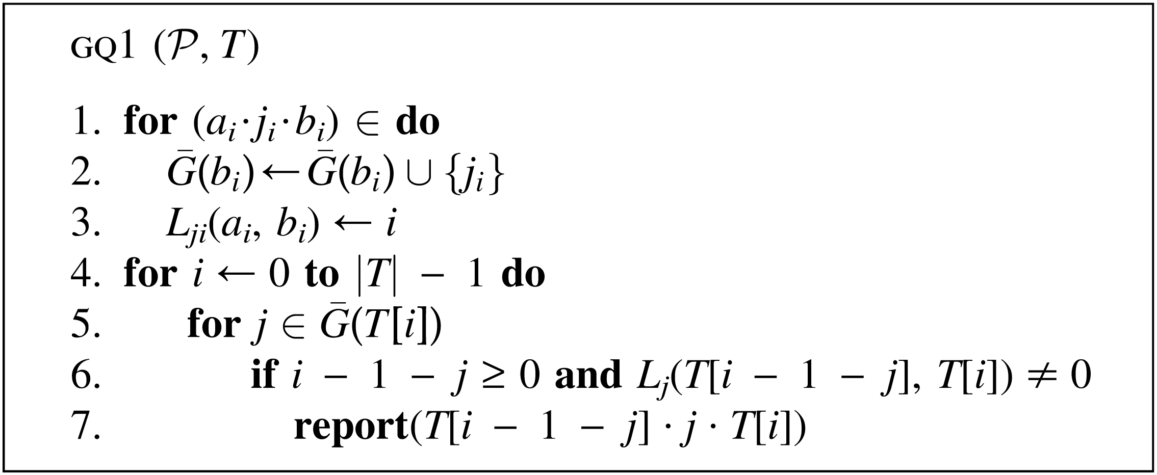
\end{document}, the LUT entry Lj(Ti−j−1, Ti), where Ti−j−1 is the substring of length h at distance j + 1 from Ti. It traverses the associated list of patterns and reports each match in overall O(1) time. The algorithm for h = 1 is depicted in Figure 2.
The gq1 algorithm, with h = 1, for the string-matching problem with gapped 2-gram patterns.
The text scanning plus text packing is performed in O(\documentclass{aastex}\usepackage{amsbsy}\usepackage{amsfonts}\usepackage{amssymb}\usepackage{bm}\usepackage{mathrsfs}\usepackage{pifont}\usepackage{stmaryrd}\usepackage{textcomp}\usepackage{portland, xspace}\usepackage{amsmath, amsxtra}\pagestyle{empty}\DeclareMathSizes{10}{9}{7}{6}\begin{document}
$$n + ng_{{ \rm span}} ( { \cal P} ) / h + occ )$$
\end{document} time. Concerning the preprocessing time, for h = 1 we can build the LUT in time O(\documentclass{aastex}\usepackage{amsbsy}\usepackage{amsfonts}\usepackage{amssymb}\usepackage{bm}\usepackage{mathrsfs}\usepackage{pifont}\usepackage{stmaryrd}\usepackage{textcomp}\usepackage{portland, xspace}\usepackage{amsmath, amsxtra}\pagestyle{empty}\DeclareMathSizes{10}{9}{7}{6}\begin{document}
$$\sigma^2 g_{{ \rm span}} ( { \cal P} ) + \mid ( { \cal P} ) \mid )$$
\end{document}). For h >1, observe that there are at most h matching patterns per slot of Lj, and they can be found in O(h) time if we build the LUT for h = 1 and use it to resolve in constant time membership queries on \documentclass{aastex}\usepackage{amsbsy}\usepackage{amsfonts}\usepackage{amssymb}\usepackage{bm}\usepackage{mathrsfs}\usepackage{pifont}\usepackage{stmaryrd}\usepackage{textcomp}\usepackage{portland, xspace}\usepackage{amsmath, amsxtra}\pagestyle{empty}\DeclareMathSizes{10}{9}{7}{6}\begin{document}
$${ \cal P}$$
\end{document}. Hence, the total time required to build the LUT is O(\documentclass{aastex}\usepackage{amsbsy}\usepackage{amsfonts}\usepackage{amssymb}\usepackage{bm}\usepackage{mathrsfs}\usepackage{pifont}\usepackage{stmaryrd}\usepackage{textcomp}\usepackage{portland, xspace}\usepackage{amsmath, amsxtra}\pagestyle{empty}\DeclareMathSizes{10}{9}{7}{6}\begin{document}
$$\sigma^{2h} g_{{ \rm span}} ( { \cal P} ) h + \mid { \cal P} \mid )$$
\end{document}). The space in words required for the LUT is O(\documentclass{aastex}\usepackage{amsbsy}\usepackage{amsfonts}\usepackage{amssymb}\usepackage{bm}\usepackage{mathrsfs}\usepackage{pifont}\usepackage{stmaryrd}\usepackage{textcomp}\usepackage{portland, xspace}\usepackage{amsmath, amsxtra}\pagestyle{empty}\DeclareMathSizes{10}{9}{7}{6}\begin{document}
$$\sigma^{2h} g_{{ \rm span}} ( { \cal P} ) h$$
\end{document}). An alternative approach, useful when h is large, is to compute the LUT lazily. We initialize each slot of the LUT to 0. This is fast in practice, and in theory it can also be done in constant time and with no overhead in the space complexity using the method described in Navarro (2012). Then, when the algorithm accesses a slot that is set to 0, it computes the corresponding list of patterns as described before and updates the slot value.
It is also possible to improve the performance in the average case by computing an additional array \documentclass{aastex}\usepackage{amsbsy}\usepackage{amsfonts}\usepackage{amssymb}\usepackage{bm}\usepackage{mathrsfs}\usepackage{pifont}\usepackage{stmaryrd}\usepackage{textcomp}\usepackage{portland, xspace}\usepackage{amsmath, amsxtra}\pagestyle{empty}\DeclareMathSizes{10}{9}{7}{6}\begin{document}
$$\bar{G}$$
\end{document} of size σh, where the entry \documentclass{aastex}\usepackage{amsbsy}\usepackage{amsfonts}\usepackage{amssymb}\usepackage{bm}\usepackage{mathrsfs}\usepackage{pifont}\usepackage{stmaryrd}\usepackage{textcomp}\usepackage{portland, xspace}\usepackage{amsmath, amsxtra}\pagestyle{empty}\DeclareMathSizes{10}{9}{7}{6}\begin{document}
$$\bar{G} ( S )$$
\end{document}, for \documentclass{aastex}\usepackage{amsbsy}\usepackage{amsfonts}\usepackage{amssymb}\usepackage{bm}\usepackage{mathrsfs}\usepackage{pifont}\usepackage{stmaryrd}\usepackage{textcomp}\usepackage{portland, xspace}\usepackage{amsmath, amsxtra}\pagestyle{empty}\DeclareMathSizes{10}{9}{7}{6}\begin{document}
$$S \in \Sigma^h$$
\end{document}, contains the list of gap lengths j, together with a pointer to the corresponding LUT, such that there exists \documentclass{aastex}\usepackage{amsbsy}\usepackage{amsfonts}\usepackage{amssymb}\usepackage{bm}\usepackage{mathrsfs}\usepackage{pifont}\usepackage{stmaryrd}\usepackage{textcomp}\usepackage{portland, xspace}\usepackage{amsmath, amsxtra}\pagestyle{empty}\DeclareMathSizes{10}{9}{7}{6}\begin{document}
$$S^{ \prime} \in \Sigma^h: L_j ( S^{ \prime} , S ) \neq \emptyset$$
\end{document}. In this way, we can limit the iterations, for each position i, to all the gap lengths \documentclass{aastex}\usepackage{amsbsy}\usepackage{amsfonts}\usepackage{amssymb}\usepackage{bm}\usepackage{mathrsfs}\usepackage{pifont}\usepackage{stmaryrd}\usepackage{textcomp}\usepackage{portland, xspace}\usepackage{amsmath, amsxtra}\pagestyle{empty}\DeclareMathSizes{10}{9}{7}{6}\begin{document}
$$j \in \bar{G} ( T_i )$$
\end{document}, which can be significantly less than the total number of gap lengths on average.
Note that since h ≥ 1, this algorithm can be used only for σ = o(n1/2). We can set h to an appropriate value below log n/(2⌈log σ⌉), to obtain o(\documentclass{aastex}\usepackage{amsbsy}\usepackage{amsfonts}\usepackage{amssymb}\usepackage{bm}\usepackage{mathrsfs}\usepackage{pifont}\usepackage{stmaryrd}\usepackage{textcomp}\usepackage{portland, xspace}\usepackage{amsmath, amsxtra}\pagestyle{empty}\DeclareMathSizes{10}{9}{7}{6}\begin{document}
$$n g_{{ \rm span}} ( { \cal P} ) ( \log n / \log \sigma )$$
\end{document}) words of space. With h as specified above, the LUT update time complexity can be absorbed in the search time. Overall, the algorithm works in O(\documentclass{aastex}\usepackage{amsbsy}\usepackage{amsfonts}\usepackage{amssymb}\usepackage{bm}\usepackage{mathrsfs}\usepackage{pifont}\usepackage{stmaryrd}\usepackage{textcomp}\usepackage{portland, xspace}\usepackage{amsmath, amsxtra}\pagestyle{empty}\DeclareMathSizes{10}{9}{7}{6}\begin{document}
$$n + ng_{{ \rm span}} ( { \cal P} ) \log \sigma / \log n + occ$$
\end{document}) time in the worst case.
We note that in theory, a slightly better algorithm using similar ideas is possible, which can handle a few gaps at a time if their lengths are close to each other. This algorithm is not practical though, and thus we do not present it. In general, L may be a large structure, so in practice one chooses a limit M (in words) on its size and computes the maximum h that satisfies σ2hgspan(\documentclass{aastex}\usepackage{amsbsy}\usepackage{amsfonts}\usepackage{amssymb}\usepackage{bm}\usepackage{mathrsfs}\usepackage{pifont}\usepackage{stmaryrd}\usepackage{textcomp}\usepackage{portland, xspace}\usepackage{amsmath, amsxtra}\pagestyle{empty}\DeclareMathSizes{10}{9}{7}{6}\begin{document}
$${ \cal P}$$
\end{document})h ≤ M. For example, for M = 222, gspan(\documentclass{aastex}\usepackage{amsbsy}\usepackage{amsfonts}\usepackage{amssymb}\usepackage{bm}\usepackage{mathrsfs}\usepackage{pifont}\usepackage{stmaryrd}\usepackage{textcomp}\usepackage{portland, xspace}\usepackage{amsmath, amsxtra}\pagestyle{empty}\DeclareMathSizes{10}{9}{7}{6}\begin{document}
$${ \cal P}$$
\end{document}) = 10 and σ = 4, we can safely use h = 4. If M is increased to 226, then h = 5 may be used.
4.2. The GQ2 algorithm
We now present the second algorithm, gq2. Let \documentclass{aastex}\usepackage{amsbsy}\usepackage{amsfonts}\usepackage{amssymb}\usepackage{bm}\usepackage{mathrsfs}\usepackage{pifont}\usepackage{stmaryrd}\usepackage{textcomp}\usepackage{portland, xspace}\usepackage{amsmath, amsxtra}\pagestyle{empty}\DeclareMathSizes{10}{9}{7}{6}\begin{document}
$${ \cal P}_a$$
\end{document} be the set of all gapped 2-gram patterns in \documentclass{aastex}\usepackage{amsbsy}\usepackage{amsfonts}\usepackage{amssymb}\usepackage{bm}\usepackage{mathrsfs}\usepackage{pifont}\usepackage{stmaryrd}\usepackage{textcomp}\usepackage{portland, xspace}\usepackage{amsmath, amsxtra}\pagestyle{empty}\DeclareMathSizes{10}{9}{7}{6}\begin{document}
$${ \cal P}$$
\end{document} with first symbol equal to a. Let also \documentclass{aastex}\usepackage{amsbsy}\usepackage{amsfonts}\usepackage{amssymb}\usepackage{bm}\usepackage{mathrsfs}\usepackage{pifont}\usepackage{stmaryrd}\usepackage{textcomp}\usepackage{portland, xspace}\usepackage{amsmath, amsxtra}\pagestyle{empty}\DeclareMathSizes{10}{9}{7}{6}\begin{document}
$$GA ( { \cal P}_a ) = ( Q , \Sigma , \delta , q_0 , F )$$
\end{document} be the nondeterministic finite automaton for the language \documentclass{aastex}\usepackage{amsbsy}\usepackage{amsfonts}\usepackage{amssymb}\usepackage{bm}\usepackage{mathrsfs}\usepackage{pifont}\usepackage{stmaryrd}\usepackage{textcomp}\usepackage{portland, xspace}\usepackage{amsmath, amsxtra}\pagestyle{empty}\DeclareMathSizes{10}{9}{7}{6}\begin{document}
$$\bigcup\nolimits_{ ( a \cdot j \cdot b ) \in { \cal P}_a} \Sigma^*a \Sigma^jb$$
\end{document} and defined as follows:
\documentclass{aastex}\usepackage{amsbsy}\usepackage{amsfonts}\usepackage{amssymb}\usepackage{bm}\usepackage{mathrsfs}\usepackage{pifont}\usepackage{stmaryrd}\usepackage{textcomp}\usepackage{portland, xspace}\usepackage{amsmath, amsxtra}\pagestyle{empty}\DeclareMathSizes{10}{9}{7}{6}\begin{document}
\begin{align*} & Q = \{ q_0 , q_1 , q_2 , \ldots , q_{g \max ( { \cal P} ) + 2} \} \\ & F = \{ q_{g \max ( { \cal P} ) + 2} \} \end{align*}
\end{document}\documentclass{aastex}\usepackage{amsbsy}\usepackage{amsfonts}\usepackage{amssymb}\usepackage{bm}\usepackage{mathrsfs}\usepackage{pifont}\usepackage{stmaryrd}\usepackage{textcomp}\usepackage{portland, xspace}\usepackage{amsmath, amsxtra}\pagestyle{empty}\DeclareMathSizes{10}{9}{7}{6}\begin{document}
\begin{align*}\delta (q_{i} , c) = \left\{ \begin{matrix} \{
q_{0} , q_{1} \} \hfill {\rm if} \ i = 0 \ { \rm and } \ c = a
\hfill \\ \{ q_{0} \} \ \hfill \quad { \rm if } \ i = 0 \ { \rm
and } \ c \neq a \hfill\\ \{ q_{i + 1} , q_{g \max ( { \cal P}_a
) + 2} \} \hfill \qquad\qquad { \rm if} \ ( a \cdot i - 1 \cdot c
) \in {\cal P}_a \ { \rm and} \ i \le g_{ \max} ( { \cal P}_a )
\hfill\\ \{ q_{g \max ( { \cal P}_a ) + 2} \} \hfill
\qquad\qquad\qquad\qquad { \rm if} \ ( a \cdot i - 1 \cdot c ) \in
{ \cal P}_a \ { \rm and} \ i = g_{ \max} ( { \cal P}_a ) + 1 \\
\{ q_{i + 1} \} \hfill \qquad { \rm if } \ 1 \le i \le g_{ \max}
\ ( { \cal P}_a ) \hfill \\ \emptyset \hfill { \rm
otherwise}\hfill
\end{matrix}\right.
\end{align*}
\end{document}
The main idea is to run the automata \documentclass{aastex}\usepackage{amsbsy}\usepackage{amsfonts}\usepackage{amssymb}\usepackage{bm}\usepackage{mathrsfs}\usepackage{pifont}\usepackage{stmaryrd}\usepackage{textcomp}\usepackage{portland, xspace}\usepackage{amsmath, amsxtra}\pagestyle{empty}\DeclareMathSizes{10}{9}{7}{6}\begin{document}
$$GA ( { \cal P}_{c_1} ) , \ldots , GA ( { \cal P}_{c_ \sigma} )$$
\end{document} in parallel over the text T, using bit-parallelism (Baeza-Yates and Gonnet, 1992).
For each automaton, we represent only the states \documentclass{aastex}\usepackage{amsbsy}\usepackage{amsfonts}\usepackage{amssymb}\usepackage{bm}\usepackage{mathrsfs}\usepackage{pifont}\usepackage{stmaryrd}\usepackage{textcomp}\usepackage{portland, xspace}\usepackage{amsmath, amsxtra}\pagestyle{empty}\DeclareMathSizes{10}{9}{7}{6}\begin{document}
$$q_1 , \ldots , q_{g_{ \max} ({ \cal P}) + 1}$$
\end{document}. First, the algorithm encodes the subset of the states of GA\documentclass{aastex}\usepackage{amsbsy}\usepackage{amsfonts}\usepackage{amssymb}\usepackage{bm}\usepackage{mathrsfs}\usepackage{pifont}\usepackage{stmaryrd}\usepackage{textcomp}\usepackage{portland, xspace}\usepackage{amsmath, amsxtra}\pagestyle{empty}\DeclareMathSizes{10}{9}{7}{6}\begin{document}
$$( { \cal P}_a$$
\end{document}) with an outgoing transition to the final state labeled by c, for each \documentclass{aastex}\usepackage{amsbsy}\usepackage{amsfonts}\usepackage{amssymb}\usepackage{bm}\usepackage{mathrsfs}\usepackage{pifont}\usepackage{stmaryrd}\usepackage{textcomp}\usepackage{portland, xspace}\usepackage{amsmath, amsxtra}\pagestyle{empty}\DeclareMathSizes{10}{9}{7}{6}\begin{document}
$$c \in \Sigma$$
\end{document}, in a set Ba(c) defined as follows:
\documentclass{aastex}\usepackage{amsbsy}\usepackage{amsfonts}\usepackage{amssymb}\usepackage{bm}\usepackage{mathrsfs}\usepackage{pifont}\usepackage{stmaryrd}\usepackage{textcomp}\usepackage{portland, xspace}\usepackage{amsmath, amsxtra}\pagestyle{empty}\DeclareMathSizes{10}{9}{7}{6}\begin{document}
\begin{align*}B_a ( c ) = \{ j \ \mid \ \delta ( q_{j + 1} , c ) \cap F \neq \emptyset \} .\end{align*}
\end{document}
It is easy to see that the state qj+1 of GA(\documentclass{aastex}\usepackage{amsbsy}\usepackage{amsfonts}\usepackage{amssymb}\usepackage{bm}\usepackage{mathrsfs}\usepackage{pifont}\usepackage{stmaryrd}\usepackage{textcomp}\usepackage{portland, xspace}\usepackage{amsmath, amsxtra}\pagestyle{empty}\DeclareMathSizes{10}{9}{7}{6}\begin{document}
$${ \cal P}_a$$
\end{document}) is active at position i in T iff T[i − 1 − j] = a, for \documentclass{aastex}\usepackage{amsbsy}\usepackage{amsfonts}\usepackage{amssymb}\usepackage{bm}\usepackage{mathrsfs}\usepackage{pifont}\usepackage{stmaryrd}\usepackage{textcomp}\usepackage{portland, xspace}\usepackage{amsmath, amsxtra}\pagestyle{empty}\DeclareMathSizes{10}{9}{7}{6}\begin{document}
$$j = 0 , \ldots , g_{ \max}({ \cal P})$$
\end{document}. Hence, the algorithm encodes the configuration of GA(\documentclass{aastex}\usepackage{amsbsy}\usepackage{amsfonts}\usepackage{amssymb}\usepackage{bm}\usepackage{mathrsfs}\usepackage{pifont}\usepackage{stmaryrd}\usepackage{textcomp}\usepackage{portland, xspace}\usepackage{amsmath, amsxtra}\pagestyle{empty}\DeclareMathSizes{10}{9}{7}{6}\begin{document}
$${ \cal P}_a$$
\end{document}) at position i in T in a set \documentclass{aastex}\usepackage{amsbsy}\usepackage{amsfonts}\usepackage{amssymb}\usepackage{bm}\usepackage{mathrsfs}\usepackage{pifont}\usepackage{stmaryrd}\usepackage{textcomp}\usepackage{portland, xspace}\usepackage{amsmath, amsxtra}\pagestyle{empty}\DeclareMathSizes{10}{9}{7}{6}\begin{document}
$$D_a^i$$
\end{document} defined as follows:
\documentclass{aastex}\usepackage{amsbsy}\usepackage{amsfonts}\usepackage{amssymb}\usepackage{bm}\usepackage{mathrsfs}\usepackage{pifont}\usepackage{stmaryrd}\usepackage{textcomp}\usepackage{portland, xspace}\usepackage{amsmath, amsxtra}\pagestyle{empty}\DeclareMathSizes{10}{9}{7}{6}\begin{document}
\begin{align*}D_a^i = \{ 0 \le j \le g_{ \max} ( { \cal P}_a ) \ \mid \ T [ i - 1 - j ] = a \} .\end{align*}
\end{document}
Given the sets Ba(c) and \documentclass{aastex}\usepackage{amsbsy}\usepackage{amsfonts}\usepackage{amssymb}\usepackage{bm}\usepackage{mathrsfs}\usepackage{pifont}\usepackage{stmaryrd}\usepackage{textcomp}\usepackage{portland, xspace}\usepackage{amsmath, amsxtra}\pagestyle{empty}\DeclareMathSizes{10}{9}{7}{6}\begin{document}
$$D_a^i$$
\end{document}, for all \documentclass{aastex}\usepackage{amsbsy}\usepackage{amsfonts}\usepackage{amssymb}\usepackage{bm}\usepackage{mathrsfs}\usepackage{pifont}\usepackage{stmaryrd}\usepackage{textcomp}\usepackage{portland, xspace}\usepackage{amsmath, amsxtra}\pagestyle{empty}\DeclareMathSizes{10}{9}{7}{6}\begin{document}
$$a , c \in \Sigma$$
\end{document}, as defined above, it holds that a gapped 2-gram (p1·j·p2) has an occurrence at position i in T iff p2 = T[i] and \documentclass{aastex}\usepackage{amsbsy}\usepackage{amsfonts}\usepackage{amssymb}\usepackage{bm}\usepackage{mathrsfs}\usepackage{pifont}\usepackage{stmaryrd}\usepackage{textcomp}\usepackage{portland, xspace}\usepackage{amsmath, amsxtra}\pagestyle{empty}\DeclareMathSizes{10}{9}{7}{6}\begin{document}
$$j \in D_{p_1}^i \cap B_{p_1} ( p_2 )$$
\end{document}. The list of gapped 2-gram patterns occurring at position i can thus be computed by iterating over all the elements j in \documentclass{aastex}\usepackage{amsbsy}\usepackage{amsfonts}\usepackage{amssymb}\usepackage{bm}\usepackage{mathrsfs}\usepackage{pifont}\usepackage{stmaryrd}\usepackage{textcomp}\usepackage{portland, xspace}\usepackage{amsmath, amsxtra}\pagestyle{empty}\DeclareMathSizes{10}{9}{7}{6}\begin{document}
$$D_a^i \cap B_a ( T [ i ] )$$
\end{document}, for all \documentclass{aastex}\usepackage{amsbsy}\usepackage{amsfonts}\usepackage{amssymb}\usepackage{bm}\usepackage{mathrsfs}\usepackage{pifont}\usepackage{stmaryrd}\usepackage{textcomp}\usepackage{portland, xspace}\usepackage{amsmath, amsxtra}\pagestyle{empty}\DeclareMathSizes{10}{9}{7}{6}\begin{document}
$$a \in \Sigma$$
\end{document}. The set \documentclass{aastex}\usepackage{amsbsy}\usepackage{amsfonts}\usepackage{amssymb}\usepackage{bm}\usepackage{mathrsfs}\usepackage{pifont}\usepackage{stmaryrd}\usepackage{textcomp}\usepackage{portland, xspace}\usepackage{amsmath, amsxtra}\pagestyle{empty}\DeclareMathSizes{10}{9}{7}{6}\begin{document}
$$D_a^i$$
\end{document} can be computed by using the following recurrence:
\documentclass{aastex}\usepackage{amsbsy}\usepackage{amsfonts}\usepackage{amssymb}\usepackage{bm}\usepackage{mathrsfs}\usepackage{pifont}\usepackage{stmaryrd}\usepackage{textcomp}\usepackage{portland, xspace}\usepackage{amsmath, amsxtra}\pagestyle{empty}\DeclareMathSizes{10}{9}{7}{6}\begin{document}
\begin{align*}D_a^i = \{ 0 \le j \le g_{ \max} ( { \cal P}_a ) \ \mid \ ( j = 0 \ { \rm and } \ T [ i - 1 ] = a ) \ { \rm or} \ j - 1 \in D_a^{i - 1} \} \tag{1}\end{align*}
\end{document}
Let size(a) = gmax(\documentclass{aastex}\usepackage{amsbsy}\usepackage{amsfonts}\usepackage{amssymb}\usepackage{bm}\usepackage{mathrsfs}\usepackage{pifont}\usepackage{stmaryrd}\usepackage{textcomp}\usepackage{portland, xspace}\usepackage{amsmath, amsxtra}\pagestyle{empty}\DeclareMathSizes{10}{9}{7}{6}\begin{document}$${ \cal P}_a$$\end{document}) + 1, if \documentclass{aastex}\usepackage{amsbsy}\usepackage{amsfonts}\usepackage{amssymb}\usepackage{bm}\usepackage{mathrsfs}\usepackage{pifont}\usepackage{stmaryrd}\usepackage{textcomp}\usepackage{portland, xspace}\usepackage{amsmath, amsxtra}\pagestyle{empty}\DeclareMathSizes{10}{9}{7}{6}\begin{document}
$${{\cal P}_a} \neq \emptyset$$\end{document}, and to 0 otherwise. Let \documentclass{aastex}\usepackage{amsbsy}\usepackage{amsfonts}\usepackage{amssymb}\usepackage{bm}\usepackage{mathrsfs}\usepackage{pifont}\usepackage{stmaryrd}\usepackage{textcomp}\usepackage{portland, xspace}\usepackage{amsmath, amsxtra}\pagestyle{empty}\DeclareMathSizes{10}{9}{7}{6}\begin{document}
$$\ell = \sum\nolimits_{i = 1}^{ \sigma}{{ \rm size}} ( c_i )$$
\end{document} and let also \documentclass{aastex}\usepackage{amsbsy}\usepackage{amsfonts}\usepackage{amssymb}\usepackage{bm}\usepackage{mathrsfs}\usepackage{pifont}\usepackage{stmaryrd}\usepackage{textcomp}\usepackage{portland, xspace}\usepackage{amsmath, amsxtra}\pagestyle{empty}\DeclareMathSizes{10}{9}{7}{6}\begin{document}
$${ \rm p o s} ( c_k ) = \sum\nolimits_{i = 0}^{k - 1} {\rm size} ( c_i )$$\end{document}. The algorithm maintains the sets \documentclass{aastex}\usepackage{amsbsy}\usepackage{amsfonts}\usepackage{amssymb}\usepackage{bm}\usepackage{mathrsfs}\usepackage{pifont}\usepackage{stmaryrd}\usepackage{textcomp}\usepackage{portland, xspace}\usepackage{amsmath, amsxtra}\pagestyle{empty}\DeclareMathSizes{10}{9}{7}{6}\begin{document}
$${ D}_a^i$$
\end{document} packed in a bit-vector Di of size ℓ. Each position 0 ≤ j ≤ gmax(\documentclass{aastex}\usepackage{amsbsy}\usepackage{amsfonts}\usepackage{amssymb}\usepackage{bm}\usepackage{mathrsfs}\usepackage{pifont}\usepackage{stmaryrd}\usepackage{textcomp}\usepackage{portland, xspace}\usepackage{amsmath, amsxtra}\pagestyle{empty}\DeclareMathSizes{10}{9}{7}{6}\begin{document}
$${ \cal P}_a$$
\end{document}) in \documentclass{aastex}\usepackage{amsbsy}\usepackage{amsfonts}\usepackage{amssymb}\usepackage{bm}\usepackage{mathrsfs}\usepackage{pifont}\usepackage{stmaryrd}\usepackage{textcomp}\usepackage{portland, xspace}\usepackage{amsmath, amsxtra}\pagestyle{empty}\DeclareMathSizes{10}{9}{7}{6}\begin{document}
$$D_a^i$$
\end{document} is mapped onto bit j + pos(a) in the corresponding bit-vector. For each \documentclass{aastex}\usepackage{amsbsy}\usepackage{amsfonts}\usepackage{amssymb}\usepackage{bm}\usepackage{mathrsfs}\usepackage{pifont}\usepackage{stmaryrd}\usepackage{textcomp}\usepackage{portland, xspace}\usepackage{amsmath, amsxtra}\pagestyle{empty}\DeclareMathSizes{10}{9}{7}{6}\begin{document}
$$c \in \Sigma$$
\end{document}, the sets Ba(c) are packed in a bit-vector B(c) in the same way. Let I be a bit-vector of size ℓ such that bit k is set iff pos(a) = k for some \documentclass{aastex}\usepackage{amsbsy}\usepackage{amsfonts}\usepackage{amssymb}\usepackage{bm}\usepackage{mathrsfs}\usepackage{pifont}\usepackage{stmaryrd}\usepackage{textcomp}\usepackage{portland, xspace}\usepackage{amsmath, amsxtra}\pagestyle{empty}\DeclareMathSizes{10}{9}{7}{6}\begin{document}
$$a \in \Sigma$$
\end{document}. Then, the vector D can be maintained, based on recurrence 1, using the following bitwise operations:
\documentclass{aastex}\usepackage{amsbsy}\usepackage{amsfonts}\usepackage{amssymb}\usepackage{bm}\usepackage{mathrsfs}\usepackage{pifont}\usepackage{stmaryrd}\usepackage{textcomp}\usepackage{portland, xspace}\usepackage{amsmath, amsxtra}\pagestyle{empty}\DeclareMathSizes{10}{9}{7}{6}\begin{document}
\begin{align*}{D}_i \leftarrow (({D}_{i - 1} \ll 1) \ \& \sim {I}) \mid
{F}\end{align*}
\end{document}
where F = 1 ≪ pos(T[i − 1]), if size(T[i − 1]) > 0, and to 0 otherwise. Since the value of \documentclass{aastex}\usepackage{amsbsy}\usepackage{amsfonts}\usepackage{amssymb}\usepackage{bm}\usepackage{mathrsfs}\usepackage{pifont}\usepackage{stmaryrd}\usepackage{textcomp}\usepackage{portland, xspace}\usepackage{amsmath, amsxtra}\pagestyle{empty}\DeclareMathSizes{10}{9}{7}{6}\begin{document}
$$D_a^i$$
\end{document} depends only on \documentclass{aastex}\usepackage{amsbsy}\usepackage{amsfonts}\usepackage{amssymb}\usepackage{bm}\usepackage{mathrsfs}\usepackage{pifont}\usepackage{stmaryrd}\usepackage{textcomp}\usepackage{portland, xspace}\usepackage{amsmath, amsxtra}\pagestyle{empty}\DeclareMathSizes{10}{9}{7}{6}\begin{document}
$$D_a^{i - 1}$$
\end{document}, we can maintain one vector only and update it using the above formula. To report all the occurrences of the patterns at a given position i in T, the algorithm iterates over all the bits set in D & B(T[i]) by repetitively computing the index of the highest bit set and masking it until there are no more bits set. Given a bit index k, it is not hard to see that the corresponding gap is equal to \documentclass{aastex}\usepackage{amsbsy}\usepackage{amsfonts}\usepackage{amssymb}\usepackage{bm}\usepackage{mathrsfs}\usepackage{pifont}\usepackage{stmaryrd}\usepackage{textcomp}\usepackage{portland, xspace}\usepackage{amsmath, amsxtra}\pagestyle{empty}\DeclareMathSizes{10}{9}{7}{6}\begin{document}
$$k - \max \{ {\rm pos} ( a ) \le k , a \in \Sigma \} $$
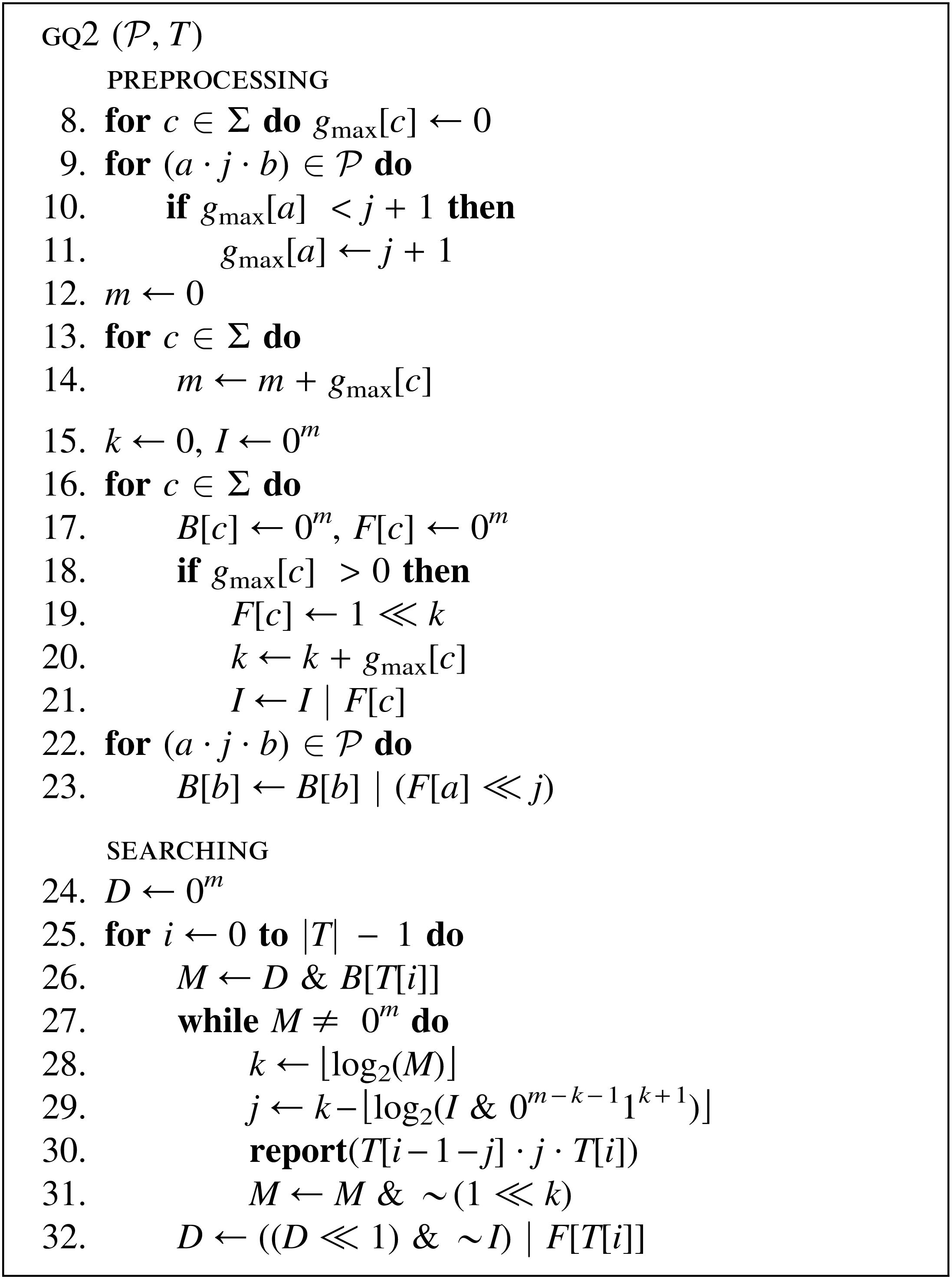
\end{document}. This translates into computing the index of the highest bit set in I & 0m−k−11k+1. Hence, for each bit k set in D & B(T[i]), the algorithm reports an occurrence of (T[i − 1 − j] · j · T[i]), where j = k − ⌊log2(I & 0m−k−11k+1)⌋. The algorithm is depicted in Figure 3.
The gq2 algorithm for the string-matching problem with gapped 2-gram patterns.
Note that gmax(\documentclass{aastex}\usepackage{amsbsy}\usepackage{amsfonts}\usepackage{amssymb}\usepackage{bm}\usepackage{mathrsfs}\usepackage{pifont}\usepackage{stmaryrd}\usepackage{textcomp}\usepackage{portland, xspace}\usepackage{amsmath, amsxtra}\pagestyle{empty}\DeclareMathSizes{10}{9}{7}{6}\begin{document}
$${ \cal P}$$
\end{document}) ≤ ℓ ≤ σgmax(\documentclass{aastex}\usepackage{amsbsy}\usepackage{amsfonts}\usepackage{amssymb}\usepackage{bm}\usepackage{mathrsfs}\usepackage{pifont}\usepackage{stmaryrd}\usepackage{textcomp}\usepackage{portland, xspace}\usepackage{amsmath, amsxtra}\pagestyle{empty}\DeclareMathSizes{10}{9}{7}{6}\begin{document}
$${ \cal P}$$
\end{document}). However, it is easy to replace the gmax(\documentclass{aastex}\usepackage{amsbsy}\usepackage{amsfonts}\usepackage{amssymb}\usepackage{bm}\usepackage{mathrsfs}\usepackage{pifont}\usepackage{stmaryrd}\usepackage{textcomp}\usepackage{portland, xspace}\usepackage{amsmath, amsxtra}\pagestyle{empty}\DeclareMathSizes{10}{9}{7}{6}\begin{document}
$${ \cal P}$$
\end{document}) term with gsize(\documentclass{aastex}\usepackage{amsbsy}\usepackage{amsfonts}\usepackage{amssymb}\usepackage{bm}\usepackage{mathrsfs}\usepackage{pifont}\usepackage{stmaryrd}\usepackage{textcomp}\usepackage{portland, xspace}\usepackage{amsmath, amsxtra}\pagestyle{empty}\DeclareMathSizes{10}{9}{7}{6}\begin{document}
$${ \cal P}$$
\end{document}): we reduce the size of the bit-vectors of each automaton GA(\documentclass{aastex}\usepackage{amsbsy}\usepackage{amsfonts}\usepackage{amssymb}\usepackage{bm}\usepackage{mathrsfs}\usepackage{pifont}\usepackage{stmaryrd}\usepackage{textcomp}\usepackage{portland, xspace}\usepackage{amsmath, amsxtra}\pagestyle{empty}\DeclareMathSizes{10}{9}{7}{6}\begin{document}
$${ \cal P}_a$$
\end{document}) by gmin(\documentclass{aastex}\usepackage{amsbsy}\usepackage{amsfonts}\usepackage{amssymb}\usepackage{bm}\usepackage{mathrsfs}\usepackage{pifont}\usepackage{stmaryrd}\usepackage{textcomp}\usepackage{portland, xspace}\usepackage{amsmath, amsxtra}\pagestyle{empty}\DeclareMathSizes{10}{9}{7}{6}\begin{document}
$${ \cal P}$$
\end{document}) bits by representing only the states \documentclass{aastex}\usepackage{amsbsy}\usepackage{amsfonts}\usepackage{amssymb}\usepackage{bm}\usepackage{mathrsfs}\usepackage{pifont}\usepackage{stmaryrd}\usepackage{textcomp}\usepackage{portland, xspace}\usepackage{amsmath, amsxtra}\pagestyle{empty}\DeclareMathSizes{10}{9}{7}{6}\begin{document}
$$q_{g \min ( { \cal P} ) + 1} , \ldots , q_{g \max ( { \cal P}_a ) + 1}$$
\end{document} (we decided not to include this improvement into the description for simplicity). For each position in the text, the bitwise operations needed to update the D vector and report the occurrences have to access ⌈ℓ/w ⌉ words. Hence, the time complexity of the searching phase of the algorithm is O(n⌈ℓ/w⌉ + occ), where occ is the number of occurrences of the patterns in the text. The space complexity is O(σ⌈ℓ/w⌉).
5. Results
In this section, we evaluate the performance of our method. All the algorithms, except pma, whose source code was kindly provided by the authors, have been implemented in the C++ programming language and compiled with the GNU C++ Compiler 4.4, using the options −03. The test machine was a 3 GHz Intel Core 2 Quad running Ubuntu 10.04, and running times were measured with the getrusage function. We performed two experiments to assess the performance of our motif-matching tool and of our algorithms for gapped q-gram patterns, respectively.
The first experiment consisted in running our motif finder, named fmf (FMM-motif-finder), with real FMM motifs on a human genome chromosome of 249, 250, 621 base pairs. Note that the particular type of sequence is not relevant for the benchmark. The motifs used were downloaded from the Segal Lab website. These motifs include features that span one and two positions. The features that span one position are basically a PWM matrix and are naively matched since optimizations like the lookahead technique cannot be applied in this more general model (see Pizzi and Ukkonen, 2008, for a survey on PWM matching algorithms). For long motifs (>20) we use the superalphabet technique described in Pizzi et al. (2011). The features that span two positions are matched using the gq2 algorithm if gsize(\documentclass{aastex}\usepackage{amsbsy}\usepackage{amsfonts}\usepackage{amssymb}\usepackage{bm}\usepackage{mathrsfs}\usepackage{pifont}\usepackage{stmaryrd}\usepackage{textcomp}\usepackage{portland, xspace}\usepackage{amsmath, amsxtra}\pagestyle{empty}\DeclareMathSizes{10}{9}{7}{6}\begin{document}
$${ \cal P}$$
\end{document}) is small (which is always the case for short motifs, since gsize(\documentclass{aastex}\usepackage{amsbsy}\usepackage{amsfonts}\usepackage{amssymb}\usepackage{bm}\usepackage{mathrsfs}\usepackage{pifont}\usepackage{stmaryrd}\usepackage{textcomp}\usepackage{portland, xspace}\usepackage{amsmath, amsxtra}\pagestyle{empty}\DeclareMathSizes{10}{9}{7}{6}\begin{document}
$${ \cal P}$$
\end{document}) can be at most equal to the motif length), and with gq1 otherwise. For a motif of length m the program computes the total score of each substring of length m of the sequence. Table 1 lists the running times for different motifs and also the corresponding motif length and the number of features that span two positions. The table also lists the running time of a naive scan in which all the features that span two positions are matched naively, that is, each site is checked for all the features. The results show that our method is fast and is thus suitable in practice, and about three times faster than a naive approach. To show the overhead due to searching for two-position features and also for naively matching the PWM matrix, we list in Table 2 the running times of the MOODS software (Korhonen et al., 2009), a suite of algorithms for PWM matching, to search for different PWM motifs downloaded from the JASPAR database. The results show that PWM matching is faster by a factor between 1.4 and 2, which, although not negligible, is an acceptable trade-off for dealing with the more complex FMM model.
Running Times in Seconds of FMM Motif Finder on a Human Genome Chromosome of 225, 280, 621 Base Pairs for Different Motifs
Motif
Motif length
Features
Time
Naive alg. time
NRSF
23
20
10.04
32.75
CTCF
19
20
9.26
30.47
STAT1_U
17
20
9.15
27.77
E2F4_Boyer
14
15
7.96
22.39
OCT4_Boyer
15
15
9.45
25.60
SOX2_Boyer
12
16
8.30
24.56
Running Times in Seconds of the MOODS Software on a Human Genome Chromosome of 225, 280, 621 Base Pairs for Different PWM Motifs with a p-value of 10−2
Motif
Motif length
Time
Ar
22
7.83
REST
19
8.96
NR1H2
17
7.35
RXRA::VDR
15
7.03
br_Z1
14
5.80
dl_1
12
4.54
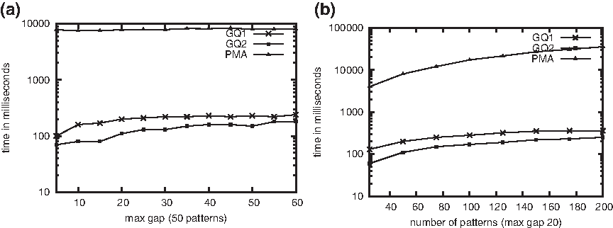
In the second experiment, we compared the gq1 and gq2 algorithms with the pma algorithm (Haapasalo et al., 2011), which is one of the best practical methods for the VLG problem. The experiment consisted in searching for a set of randomly generated gapped q-gram patterns on the genome sequence of 4, 638, 690 base pairs of Escherichia coli.Figure 4a shows the running times for searching a set of randomly generated 2-gram patterns with a fixed number of patterns equal to 50 and such that the maximum gap varies between 5 and 60. Figure 4b shows the running times for searching a set of randomly generated 2-gram patterns with a fixed maximum gap of 20 and such that the number of patterns varies between 25 and 200. We used a logarithmic scale on the y axis. The experimental results show that the new algorithms are significantly faster (up to 50 times) than the pma algorithm in this particular scenario. The approach based on locating the occurrences of the key words does not scale well when all the key words, and in particular, the first key word, are of length 1. Note that in the general case of arbitrary length key words, the pma algorithm is very fast (Haapasalo et al., 2011). In all the results, the gq2 algorithm is slightly faster than the gq1 algorithm. This is expected because in all the experiments gspan(\documentclass{aastex}\usepackage{amsbsy}\usepackage{amsfonts}\usepackage{amssymb}\usepackage{bm}\usepackage{mathrsfs}\usepackage{pifont}\usepackage{stmaryrd}\usepackage{textcomp}\usepackage{portland, xspace}\usepackage{amsmath, amsxtra}\pagestyle{empty}\DeclareMathSizes{10}{9}{7}{6}\begin{document}
$${ \cal P}$$
\end{document}) is almost equal to gsize(\documentclass{aastex}\usepackage{amsbsy}\usepackage{amsfonts}\usepackage{amssymb}\usepackage{bm}\usepackage{mathrsfs}\usepackage{pifont}\usepackage{stmaryrd}\usepackage{textcomp}\usepackage{portland, xspace}\usepackage{amsmath, amsxtra}\pagestyle{empty}\DeclareMathSizes{10}{9}{7}{6}\begin{document}
$${ \cal P}$$
\end{document}), and thus the word-level parallelism pays off. To show the difference between the two algorithms for a sparse set of gaps, we performed another experiment in which the number of patterns is fixed at 25 and the maximum gap varies between 50 and 150, so that, for increasing values of the maximum gap, gspan(\documentclass{aastex}\usepackage{amsbsy}\usepackage{amsfonts}\usepackage{amssymb}\usepackage{bm}\usepackage{mathrsfs}\usepackage{pifont}\usepackage{stmaryrd}\usepackage{textcomp}\usepackage{portland, xspace}\usepackage{amsmath, amsxtra}\pagestyle{empty}\DeclareMathSizes{10}{9}{7}{6}\begin{document}$${ \cal P}$$\end{document}) is always 25 at most while gsize(\documentclass{aastex}\usepackage{amsbsy}\usepackage{amsfonts}\usepackage{amssymb}\usepackage{bm}\usepackage{mathrsfs}\usepackage{pifont}\usepackage{stmaryrd}\usepackage{textcomp}\usepackage{portland, xspace}\usepackage{amsmath, amsxtra}\pagestyle{empty}\DeclareMathSizes{10}{9}{7}{6}\begin{document}$${ \cal P}$$\end{document}) increases. The results, depicted in Figure 5, show that in this scenario the gq1 algorithm is faster than the gq2 algorithm when the maximum gap is at least four times the number of patterns.
Experimental results on a genome sequence of Escherichia coli with randomly generated gapped 2-gram patterns obtained for (a) varying gap interval with a set of 50 patterns and (b) varying number of patterns with maximum gap 20.
Comparison of the gq1 and gq2 algorithms for a sparse set of gaps.
6. Conclusions
We presented a method for the problem of finding all the locations in DNA sequences that match a motif describing transcription factor binding sites under the feature motif model. Our approach is based on reducing the problem to the one of matching a set of gapped q-gram patterns, where a gapped q-gram pattern is a sequence of q symbols such that there is a gap of fixed length between each two consecutive symbols. To this end, we presented novel algorithms for this problem in the q = 2 case, which we believe could be of independent interest. We note that a more general but slower algorithm that works for any q is possible using a similar approach. The experimental results show that our method achieves very good performance and is thus effective. It is worth observing that any PWM motif can be expressed in the FMM model, so there is no drawback in the use of this model.
Footnotes
7. Acknowledgments
This work was supported by the Academy of Finland, grant 118653 (ALGODAN), and by the Polish Ministry of Science and Higher Education, project N N516 441938.
8. Disclosure Statement
The authors declare that no competing financial interests exist.
References
1.
ArlazarovV., DinicE., KronrodM., FaradzevI.1970. On economical construction of the transitive closure of a directed graph. Soviet Math. Doklady, 11:1209–1210.
2.
Baeza-YatesR.A., GonnetG.H.1992. A new approach to text searching. Commun. ACM, 35:74–82.
3.
BiY., KimH., GuptaR., DavuluriR.V.2011. Tree-based position weight matrix approach to model transcription factor binding site profiles. PLoS ONE, 6.
4.
BilleP., GørtzI.L., VildhøjH.W., WindD.K.2010. String matching with variable length gaps, 385–394. ChávezE., LonardiS.SPIRE6393Lecture Notes in Computer Science. Springer: New York.
5.
BurgeC., KarlinS.1997. Prediction of complete gene structures in human genomic DNA. J of Mol Biol, 268:78–94.
6.
GribskovM., McLachlanA.D., EisenbergD.1987. Profile analysis: detection of distantly related proteins. Proceedings of the National Academy of Sciences, 84:4355–4358.
7.
HaapasaloT., SilvastiP., SippuS., Soisalon-SoininenE.2011. Online dictionary matching with variable-length gaps, 76–87. PardalosP.M., RebennackS.ed. SEA, Vol.6630Lecture Notes in Computer Science. Springer: New York.
8.
HallikasO., PalinK., SinjushinaN.et al.2006. Genome-wide prediction of mammalian enhancers based on analysis of transcription-factor binding affinity. Cell, 124:47–59.
9.
KorhonenJ., MartinmäkiP., PizziC.et al.2009. MOODS: fast search for position weight matrix matches in DNA sequences. Bioinformatics, 25:3181–3182.
10.
NavarroG.2012. Constant-time array initialization in little space. In Proc. XXXI International Conference of the Chilean Computer Science Society (SCCC). IEEE CS Press. In press.
11.
PizziC, UkkonenE.2008. Fast profile matching algorithms - a survey. Theor. Comput. Sci., 395:137–157.
12.
PizziC., RastasP., UkkonenE.2011. Finding significant matches of position weight matrices in linear time. IEEE/ACM Trans. Comput. Biology Bioinform., 8:69–79.
13.
SchneiderT.D., StormoG.D., GoldL., EhrenfeuchtA.1986. Information content of binding sites on nucleotide sequences. J Mol. Biol., 188:415–431.
14.
SharonE., LublinerS., SegalE.2008. A feature-based approach to modeling protein-DNA interactions. PLoS Comp. Biol., 4.
15.
SiddharthanR.2010. Dinucleotide weight matrices for predicting transcription factor binding sites: Generalizing the position weight matrix. PLoS ONE, 5.
16.
StormoG.D., ShneiderT.D., GoldL., EhrenfeuchtA.1982. Use of ‘perceptron’ algorithm to distinguish translational initiation sites in E. coli. Nucleic Acids Research, 10:2997–3011.
17.
ZhaoX., HuangH., SpeedT.P.2005. Finding short DNA motifs using permuted Markov models. J Comp. Bio., 12:894–906.
18.
ZhouQ., LiuJ.S.2004. Modeling within-motif dependence for transcription factor binding site predictions. Bioinformatics, 20:909–916.