In this article, a protein sequence of length n is embedded in a two-dimensional lattice with m (>n) points. Thus the obtained minimal energy configurations are expected to have flexible shapes in contrast to the compact rectangular conformations. To fulfill this extension, the elastic net algorithm is modified to deal with the difficulty brought by the unsymmetrical relationship between amino acids and lattice points. New set partition strategy in the embedding phase is introduced, and two local search methods are applied to overcome the multimapping phenomena. Several HP benchmark examples with up to 48 amino acids are tested to verify the effectiveness of the proposed approach.
1. Introduction
The ability to reliably and efficiently predict protein structure from sequence information will greatly simplify the tasks of interpreting the data collected by the Human Genome Project, of understanding the mechanism of hereditary and infectious diseases, of designing drugs with specific therapeutic properties, and of growing biological polymers with the specific material properties (Alena et al., 2005). However, the folding kinetics is a complicated problem and many groups are working on predicting the native state of a protein from its primary structure by computational methods.
In this article, we focus on the 2D hydrophobic-polar (2D HP) model. This model has been widely used by chemists to evaluate a new hypothesis of protein structure formation (Sail et al., 1994). This model is viewed as standard in testing efficiency of the folding algorithm (Liang and Wong, 2001). By far, many methods have been adopted to crack the simplified model such as ant colony optimization algorithm (Alena et al., 2005), self-organizing networks method (Yanikoglu and Erman, 2002), self-organizing mapping method (Zhang et al., 2005), genetic algorithm (Jiang et al., 2003; Cusfódio, 2004), Monte Carlo algorithm (Unger and Moult, 1993), evolutionary Monte Carlo method (Liang and Wong, 2001), etc. The effectiveness of these methods have been tested with many proteins for 2D HP lattice model. But currently, none of these algorithms seem to dominate the others.
From the viewpoint of applications of HP model, it is not natural to limit the native state to be a square, a rectangle, or some predetermined shapes. Therefore, this article aims to find native configuration of a protein with the number of lattice points larger than the number of amino acids. In other words, the flexible and different shapes, that is, nonrectangular structure (NRS), will be obtained.
The elastic net (EN) method, which was introduced by Durbin and Willshaw to solve the traveling salesman problem (TSP) (Durbin and Willshaw, 1987), belongs to the class of geometric neural networks. Although it is closely related to the Hopfield-Tank algorithm (Hopfield and Tank, 1985) and other neural network optimization methods, it performs as well as, or better than, those methods. The EN method has been successfully applied in pattern recognition, machine vision, and other matching problems (Simic, 1991). The EN method has the advantage of being easily parallelizable and is more versatile. This flexibility makes the EN algorithm a suitable candidate for protein structure prediction (Guo et al. 2007). But there are three fundamental differences between the 2D HP protein structure prediction and the traveling salesman problem, so it can't be applied directly to the protein folding problem. In this article, we modify the EN algorithm to simulate the protein folding on simple lattice model and to find the ground state. One difficulty of the modified EN algorithm for the 2D HP lattice model is the multimapping problem, which means that two or more amino acids visit the same lattice point when the training phase is finished. To alleviate it, we present two local search methods.
This remainder article is organized as follows: Section 2 gives a detailed description of the HP model and the energy function. A hybrid of the modified EN algorithm and local search methods is introduced in section 3. Section 4 is devoted to demonstrating and analyzing the empirical results of the proposed algorithm. Finally, a short discussion and conclusion are given in section 5.
2. The 2D Hp Model
The HP model of protein structure was first proposed by Lau and Dill in 1998 (Lau and Dill, 1998). It is based on the assumption that interactions between noncovalently bonded hydrophobic neighbors play the dominant role in the encoding of proteins in both the compactness and specific architecture stated by Dill and his colleagues in their article (Dill et al. 1995). In the HP model, twenty kinds of amino acids are classified as: hydrophobic (H for nonpolar) and hydrophilic (P for polar). Based on this classification, the primary amino acid sequence of a protein is represented as a binary string, even though some amino acids can not be clearly classified, the model disregards this fact to achieve simplicity. A folding of protein in the 2D HP model is an embedding of protein sequences in the square lattice such that adjacent amino acids occupy adjacent grid points in the lattice, and no grid point in the lattice is occupied by more than one. The H–H bond, H–P bond, and P–P bond are formed if they occupy adjacent grid points in lattice but are not adjacent in sequence. Then the self-avoiding configurations are evaluated with energies EHH = 1, EHP = 0, and EPP = 0. For the 2D HP model, the ideal structure of a protein is to maximize the number of H–H bonds such that the H points are buried in the whole globular protein, and P points are located in the surface to contact with the water molecules, which implies the compactness of the protein structure. In other words, the HP model delineates a combinatorial optimization problem: a sequence of H and P points is put into a lattice with the original ordering of the H, P points unchanged, and the number of H-H bonds maximized.
3. En Algorithm For Protein Structure
The idea of applying the EN algorithm in protein structure prediction originates from the efficient performance of EN algorithms for the traveling salesman problem (TSP). It should be noted that there are three fundamental differences between these two problems: (1) The amino acid sequence is not in a closed loop in protein structure prediction. (2) The native conformation of protein folding is with minimum free energy, not with shortest possible path. (3) Local neighbor of the amino acid chain must be maintained in the process of protein folding. However, as for the computation of the EN algorithm, these two problems have similar computation procedure, which is the main reason why we still choose a TSP model to describe such a problem.
The application of the EN algorithm encounters algorithmic and computational difficulty, since in this case the number of lattice points is larger than the number of amino acids. Some points in the lattice will not be visited, and the original order of amino acids in sequence must be unchanged. To overcome these difficulties, we introduce the lattice partition strategy and two local search schemes.
3.1. Initialization
Given a protein chain of n amino acids, \documentclass{aastex}\usepackage{amsbsy}\usepackage{amsfonts}\usepackage{amssymb}\usepackage{bm}\usepackage{mathrsfs}\usepackage{pifont}\usepackage{stmaryrd}\usepackage{textcomp}\usepackage{portland, xspace}\usepackage{amsmath, amsxtra}\pagestyle{empty}\DeclareMathSizes{10}{9}{7}{6}\begin{document}
$$r = \{ r_{1} , r_{2} , \cdots , r_{n} \} \subset \{ H , P \} $$
\end{document} is an abstract of the amino acid sequence. Denote
\documentclass{aastex}\usepackage{amsbsy}\usepackage{amsfonts}\usepackage{amssymb}\usepackage{bm}\usepackage{mathrsfs}\usepackage{pifont}\usepackage{stmaryrd}\usepackage{textcomp}\usepackage{portland, xspace}\usepackage{amsmath, amsxtra}\pagestyle{empty}\DeclareMathSizes{10}{9}{7}{6}\begin{document}
\begin{align*}f ( i ) = \begin{cases}0 \quad r_{i} = P \\ 1 \quad r_{i} = H\end{cases} \tag{1}\end{align*}
\end{document}
Set a lattice L with m points where m > n. Suppose that m = p × q where p and q are odd numbers. \documentclass{aastex}\usepackage{amsbsy}\usepackage{amsfonts}\usepackage{amssymb}\usepackage{bm}\usepackage{mathrsfs}\usepackage{pifont}\usepackage{stmaryrd}\usepackage{textcomp}\usepackage{portland, xspace}\usepackage{amsmath, amsxtra}\pagestyle{empty}\DeclareMathSizes{10}{9}{7}{6}\begin{document}
$$S = \{S_{1} , S_{2} , \cdots , S_{m} \} $$
\end{document} is a vector set where Si = (xi, yi) denotes the coordinate of lattice point \documentclass{aastex}\usepackage{amsbsy}\usepackage{amsfonts}\usepackage{amssymb}\usepackage{bm}\usepackage{mathrsfs}\usepackage{pifont}\usepackage{stmaryrd}\usepackage{textcomp}\usepackage{portland, xspace}\usepackage{amsmath, amsxtra}\pagestyle{empty}\DeclareMathSizes{10}{9}{7}{6}\begin{document}
$$i , x_ { i } \in \{ 0 , \pm 1 , \pm 2 , \cdots , \pm \frac {p - 1} {2} \} $$
\end{document} and \documentclass{aastex}\usepackage{amsbsy}\usepackage{amsfonts}\usepackage{amssymb}\usepackage{bm}\usepackage{mathrsfs}\usepackage{pifont}\usepackage{stmaryrd}\usepackage{textcomp}\usepackage{portland, xspace}\usepackage{amsmath, amsxtra}\pagestyle{empty}\DeclareMathSizes{10}{9}{7}{6}\begin{document}
$$y_ { i } \in \{ 0 , \pm 1 , \pm 2 , \cdots , \pm \frac { q - 1 } {2} \} , i = 1 , 2 , \cdots , m$$
\end{document}. The given protein chain will be embedded in the lattice. The initial position of amino acid sequence in the lattice is given \documentclass{aastex}\usepackage{amsbsy}\usepackage{amsfonts}\usepackage{amssymb}\usepackage{bm}\usepackage{mathrsfs}\usepackage{pifont}\usepackage{stmaryrd}\usepackage{textcomp}\usepackage{portland, xspace}\usepackage{amsmath, amsxtra}\pagestyle{empty}\DeclareMathSizes{10}{9}{7}{6}\begin{document}
$$R = \{ R_{1} , R_{2} , \cdots , R_{n} \} $$
\end{document}, Ri denotes the coordinate of the amino acid \documentclass{aastex}\usepackage{amsbsy}\usepackage{amsfonts}\usepackage{amssymb}\usepackage{bm}\usepackage{mathrsfs}\usepackage{pifont}\usepackage{stmaryrd}\usepackage{textcomp}\usepackage{portland, xspace}\usepackage{amsmath, amsxtra}\pagestyle{empty}\DeclareMathSizes{10}{9}{7}{6}\begin{document}
$$r_{i} , i = 1 , 2 , \cdots , n$$
\end{document}. The given protein chain will be embedded in the lattice L with hydrophobic amino acid near the center of the lattice as compact as possible.
3.2. Modified elastic net method
Solving the HP lattice model is an optimization problem of matching lattice points to amino acids such that (1) each lattice point is visited exactly once, (2) each amino acid only visits one lattice point, (3) the original ordering of the H and P points in sequence is unchanged in the matching phase, and (4) the folding problem is to maximize the number of nonlocal H-H bonds.
In our method, the elastic net (EN) strategy uses two different sets of zero equilibrium-length harmonic springs. The first set of n−1 springs connects the adjacent amino acids in the sequence. We refer to these as the amino acid springs. The amino acid sequence can explore different conformations in the same plane to create a route through the squares of lattice. These attractive springs serve to keep local neighbors between any two neighboring amino acids. The second set of m · n springs connects each amino acid to each vertex of lattice, these springs tend to force amino acids to occupy the vertices of the lattice.
The EN method achieves the matching constraint via an iterative procedure that computes on each cycle a Boltzman-like (Ball et al., 2002) vector function φ for the vertex springs
\documentclass{aastex}\usepackage{amsbsy}\usepackage{amsfonts}\usepackage{amssymb}\usepackage{bm}\usepackage{mathrsfs}\usepackage{pifont}\usepackage{stmaryrd}\usepackage{textcomp}\usepackage{portland, xspace}\usepackage{amsmath, amsxtra}\pagestyle{empty}\DeclareMathSizes{10}{9}{7}{6}\begin{document}
\begin{align*}\phi ( \parallel S_{j} - R_{i} \parallel , K ) ( t ) = \exp ( - ( S_{j} - R_{i} ( t ) ) ^{2} / 2K^{2} ) \tag{2}\end{align*}
\end{document}
where K is a parameter, ∥Sj − Ri∥ is computed by Equation (2). Normalizing over all n vertex springs connected to vertex j gives the following statistical vector weights for each of these springs:
\documentclass{aastex}\usepackage{amsbsy}\usepackage{amsfonts}\usepackage{amssymb}\usepackage{bm}\usepackage{mathrsfs}\usepackage{pifont}\usepackage{stmaryrd}\usepackage{textcomp}\usepackage{portland, xspace}\usepackage{amsmath, amsxtra}\pagestyle{empty}\DeclareMathSizes{10}{9}{7}{6}\begin{document}
\begin{align*}w_ { ij } ( t ) = \frac { \phi ( \parallel S_ { j } - R_ { i } \parallel , K ) ( t ) } { \sum_ { k } \phi ( \parallel S_ { j } - R_ { k } \parallel , K ) ( t ) } \tag { 3 } \end{align*}
\end{document}
These weights act as variable spring constants, and \documentclass{aastex}\usepackage{amsbsy}\usepackage{amsfonts}\usepackage{amssymb}\usepackage{bm}\usepackage{mathrsfs}\usepackage{pifont}\usepackage{stmaryrd}\usepackage{textcomp}\usepackage{portland, xspace}\usepackage{amsmath, amsxtra}\pagestyle{empty}\DeclareMathSizes{10}{9}{7}{6}\begin{document}
$$\mathop \sum \limits^{n}_{i = 1}w_{ij} ( t )$$
\end{document} is a unit vector, which presents that the sum of weights of n amino acids connected to the vertex j is 1. For the 2D HP model, low energy conformations are compact with a hydrophobic core, since the H-H interactions are awarded. The hydrophobic residues have to be buried inside to yield a low energy structure, while the hydrophilic residues are forced to the surface. For this purpose, weight values of those lattices near the center of the lattice are increased
\documentclass{aastex}\usepackage{amsbsy}\usepackage{amsfonts}\usepackage{amssymb}\usepackage{bm}\usepackage{mathrsfs}\usepackage{pifont}\usepackage{stmaryrd}\usepackage{textcomp}\usepackage{portland, xspace}\usepackage{amsmath, amsxtra}\pagestyle{empty}\DeclareMathSizes{10}{9}{7}{6}\begin{document}
\begin{align*}w_ { ij } ( t + 1 ) = \left( 1 + \frac { l - 3 } { 2l } w_ { ij } ( t ) \right) , \quad i = 1 , 2 , \cdots , n , \quad j \in D \tag { 4 } \end{align*}
\end{document}
where l = min{p, q}, \documentclass{aastex}\usepackage{amsbsy}\usepackage{amsfonts}\usepackage{amssymb}\usepackage{bm}\usepackage{mathrsfs}\usepackage{pifont}\usepackage{stmaryrd}\usepackage{textcomp}\usepackage{portland, xspace}\usepackage{amsmath, amsxtra}\pagestyle{empty}\DeclareMathSizes{10}{9}{7}{6}\begin{document}
$$D = \ { j \ \mid \ x^ { 2 } _ { j } + y_ { j } ^ { 2 } \leq \frac { l + 1 } { 2 } \ } $$
\end{document}. The EN algorithm incrementally changes the coordinates of each Rj in sequence according to the rule
\documentclass{aastex}\usepackage{amsbsy}\usepackage{amsfonts}\usepackage{amssymb}\usepackage{bm}\usepackage{mathrsfs}\usepackage{pifont}\usepackage{stmaryrd}\usepackage{textcomp}\usepackage{portland, xspace}\usepackage{amsmath, amsxtra}\pagestyle{empty}\DeclareMathSizes{10}{9}{7}{6}\begin{document}
\begin{align*} \triangle R_{1} & = ac \mathop \sum \limits_{j = 1}^{m}w_{1j} ( t ) ( S_{j} - R_{1} ( t ) ) + K \cdot at ( R_{2} ( t ) - R_{1} ( t ) ) \\ \triangle R_{n} & = ac \mathop \sum \limits_{j = 1}^{m}w_{nj} ( t ) ( S_{j} - R_{n} ( t ) ) + K \cdot at ( R_{n - 1} ( t ) - R_{n} ( t ) ) & ( 5 ) \\ \triangle R_{i} & = ac \mathop \sum \limits_{j = 1}^{m} w_{ij} ( t ) ( S_{j} - R_{i} ( t ) ) + K \cdot at ( R_{i + 1} ( t ) - 2R_{i} ( t ) - R_{i - 1} ( t ) ) \end{align*}
\end{document}\documentclass{aastex}\usepackage{amsbsy}\usepackage{amsfonts}\usepackage{amssymb}\usepackage{bm}\usepackage{mathrsfs}\usepackage{pifont}\usepackage{stmaryrd}\usepackage{textcomp}\usepackage{portland, xspace}\usepackage{amsmath, amsxtra}\pagestyle{empty}\DeclareMathSizes{10}{9}{7}{6}\begin{document}
\begin{align*}i = 2 , 3 , \cdots , n - 1\end{align*}
\end{document}
where ac and at are coefficients that control the relative strengths of vertex and amino acid springs, respectively. So the coordinate of amino acid is updated by following equation
\documentclass{aastex}\usepackage{amsbsy}\usepackage{amsfonts}\usepackage{amssymb}\usepackage{bm}\usepackage{mathrsfs}\usepackage{pifont}\usepackage{stmaryrd}\usepackage{textcomp}\usepackage{portland, xspace}\usepackage{amsmath, amsxtra}\pagestyle{empty}\DeclareMathSizes{10}{9}{7}{6}\begin{document}
\begin{align*}R_{i} ( t + 1 ) = R_{i} ( t ) + \triangle R_{i} , \quad \quad i = 1 , 2 , \cdots , n \tag{6}\end{align*}
\end{document}
To keep the bond connection of protein sequence, all weight values of amino acids ri+1 on the HP sequence are updated, after the position of amino acid ri is changed
\documentclass{aastex}\usepackage{amsbsy}\usepackage{amsfonts}\usepackage{amssymb}\usepackage{bm}\usepackage{mathrsfs}\usepackage{pifont}\usepackage{stmaryrd}\usepackage{textcomp}\usepackage{portland, xspace}\usepackage{amsmath, amsxtra}\pagestyle{empty}\DeclareMathSizes{10}{9}{7}{6}\begin{document}
\begin{align*}w_ { ( i + 1 ) j } ( t + 1 ) = \frac { w_ { ( i + 1 ) j } ( t ) + e^ { \beta } \alpha ( S_ { j } - R_ { i + 1 } ( t ) ) } { \parallel w_ { ( i + 1 ) j } ( t ) + e^ { \beta } \alpha ( S_ { j } - R_ { i + 1 } ( t ) ) \parallel } \tag { 7 } \end{align*}
\end{document}
where α and β are training parameters.
3.3. The local Search procedure I
The multimapping problem, which means that two or more amino acids visit the same lattice point when the modified EN algorithm is finished, is the main difficulty encountered by EN algorithm for the HP lattice model. It gets worse when the number of lattice points is larger. In the HP model, the conformation is invalid if any lattice point is visited by two or more amino acids. To overcome this problems, we propose the local search method I which can be simply described as follows
Step 1. According to the training result of the EN algorithm, all lattice points are classified into three subsets: \documentclass{aastex}\usepackage{amsbsy}\usepackage{amsfonts}\usepackage{amssymb}\usepackage{bm}\usepackage{mathrsfs}\usepackage{pifont}\usepackage{stmaryrd}\usepackage{textcomp}\usepackage{portland, xspace}\usepackage{amsmath, amsxtra}\pagestyle{empty}\DeclareMathSizes{10}{9}{7}{6}\begin{document}
$$C: = \{ S_{i} \mid \ \parallel S_{i} - R_{j} \parallel = 0 , \parallel S_{i} - R_{k} \parallel \neq 0 , k \in I_{n} \backslash \{ j \} , j \in I_{n} , i \in I_{m} \} $$
\end{document}, in which each lattice point \documentclass{aastex}\usepackage{amsbsy}\usepackage{amsfonts}\usepackage{amssymb}\usepackage{bm}\usepackage{mathrsfs}\usepackage{pifont}\usepackage{stmaryrd}\usepackage{textcomp}\usepackage{portland, xspace}\usepackage{amsmath, amsxtra}\pagestyle{empty}\DeclareMathSizes{10}{9}{7}{6}\begin{document}
$$S_i \in C$$
\end{document} is visited by only one amino acid j, where \documentclass{aastex}\usepackage{amsbsy}\usepackage{amsfonts}\usepackage{amssymb}\usepackage{bm}\usepackage{mathrsfs}\usepackage{pifont}\usepackage{stmaryrd}\usepackage{textcomp}\usepackage{portland, xspace}\usepackage{amsmath, amsxtra}\pagestyle{empty}\DeclareMathSizes{10}{9}{7}{6}\begin{document}
$$I_{n} = \{ 1 , 2 , \cdots , n \} , I_{m} = \{ 1 , 2 , \cdots , m \} ; M: = \{ S_{i} \mid \ \parallel S_{i} - R_{j} \parallel = 0 , \parallel S_{i} - R_{k} \parallel = 0 , j \neq k , j \in I_{n} , k \in I_{n} , i \in I_{m} \} $$
\end{document}, in which each lattice point \documentclass{aastex}\usepackage{amsbsy}\usepackage{amsfonts}\usepackage{amssymb}\usepackage{bm}\usepackage{mathrsfs}\usepackage{pifont}\usepackage{stmaryrd}\usepackage{textcomp}\usepackage{portland, xspace}\usepackage{amsmath, amsxtra}\pagestyle{empty}\DeclareMathSizes{10}{9}{7}{6}\begin{document}
$$S_i \in M$$
\end{document} is visited by two or more amino acids; \documentclass{aastex}\usepackage{amsbsy}\usepackage{amsfonts}\usepackage{amssymb}\usepackage{bm}\usepackage{mathrsfs}\usepackage{pifont}\usepackage{stmaryrd}\usepackage{textcomp}\usepackage{portland, xspace}\usepackage{amsmath, amsxtra}\pagestyle{empty}\DeclareMathSizes{10}{9}{7}{6}\begin{document}
$$P: = \{ S_{i} \mid \ \parallel S_{i} - R_{j} \parallel \neq 0 , j \in I_{n} , i \in I_{m} \} $$
\end{document}, in which each lattice point \documentclass{aastex}\usepackage{amsbsy}\usepackage{amsfonts}\usepackage{amssymb}\usepackage{bm}\usepackage{mathrsfs}\usepackage{pifont}\usepackage{stmaryrd}\usepackage{textcomp}\usepackage{portland, xspace}\usepackage{amsmath, amsxtra}\pagestyle{empty}\DeclareMathSizes{10}{9}{7}{6}\begin{document}
$$S_i \in P$$
\end{document} is not visited by any amino acid.
Step 2. According to the order of amino acids, we join the lattice point set C into a temporary chain \documentclass{aastex}\usepackage{amsbsy}\usepackage{amsfonts}\usepackage{amssymb}\usepackage{bm}\usepackage{mathrsfs}\usepackage{pifont}\usepackage{stmaryrd}\usepackage{textcomp}\usepackage{portland, xspace}\usepackage{amsmath, amsxtra}\pagestyle{empty}\DeclareMathSizes{10}{9}{7}{6}\begin{document}
$$CH: = \{ S_{i_{1}} , S_{i_{2}} , \cdots , S_{i_{ \mid CH \mid}} \} $$
\end{document} where |CH| presents the number of set CH.
Step 3. For each \documentclass{aastex}\usepackage{amsbsy}\usepackage{amsfonts}\usepackage{amssymb}\usepackage{bm}\usepackage{mathrsfs}\usepackage{pifont}\usepackage{stmaryrd}\usepackage{textcomp}\usepackage{portland, xspace}\usepackage{amsmath, amsxtra}\pagestyle{empty}\DeclareMathSizes{10}{9}{7}{6}\begin{document}
$$S_i \in M$$
\end{document}, choose one rj from all amino acids that occupy the lattice point Si, according to the ordering of which in sequence, insert Si into CH, |CH| = |CH| +1, denoted by
\documentclass{aastex}\usepackage{amsbsy}\usepackage{amsfonts}\usepackage{amssymb}\usepackage{bm}\usepackage{mathrsfs}\usepackage{pifont}\usepackage{stmaryrd}\usepackage{textcomp}\usepackage{portland, xspace}\usepackage{amsmath, amsxtra}\pagestyle{empty}\DeclareMathSizes{10}{9}{7}{6}\begin{document}
\begin{align*}CH^{ \prime} ( j ) = \{ S_{i_{1}} , \cdots , S_{i_{k}} , S_{i} ( j ) , S_{i_{ ( k + 1 ) }} , \cdots , S_{i_{ \mid CH \mid}} \} .\end{align*}
\end{document}
Step 4. Put all amino acids that do not occupy any lattice points into RS.
Step 5. For each \documentclass{aastex}\usepackage{amsbsy}\usepackage{amsfonts}\usepackage{amssymb}\usepackage{bm}\usepackage{mathrsfs}\usepackage{pifont}\usepackage{stmaryrd}\usepackage{textcomp}\usepackage{portland, xspace}\usepackage{amsmath, amsxtra}\pagestyle{empty}\DeclareMathSizes{10}{9}{7}{6}\begin{document}
$$r_{j} \in RS$$
\end{document}, choose one Si from P, according to the order of rj in sequence, insert Si into CH, |CH| = |CH| +1, denoted by
\documentclass{aastex}\usepackage{amsbsy}\usepackage{amsfonts}\usepackage{amssymb}\usepackage{bm}\usepackage{mathrsfs}\usepackage{pifont}\usepackage{stmaryrd}\usepackage{textcomp}\usepackage{portland, xspace}\usepackage{amsmath, amsxtra}\pagestyle{empty}\DeclareMathSizes{10}{9}{7}{6}\begin{document}
\begin{align*}CH^{ \prime \prime} ( i ) = \{ S_{i_{1}} , \cdots , S_{i_{k}} , S_{i} ( j ) , S_{i_{ ( k + 1 ) }} , \cdots , S_{i_{ \mid CH \mid}} \} .\end{align*}
\end{document}
Compute the length of CH″ (i), written as
\documentclass{aastex}\usepackage{amsbsy}\usepackage{amsfonts}\usepackage{amssymb}\usepackage{bm}\usepackage{mathrsfs}\usepackage{pifont}\usepackage{stmaryrd}\usepackage{textcomp}\usepackage{portland, xspace}\usepackage{amsmath, amsxtra}\pagestyle{empty}\DeclareMathSizes{10}{9}{7}{6}\begin{document}
\begin{align*} length^{ \prime} ( i ) = \mathop \sum \limits_{l =
2}^{k} \parallel S_{i_{l}} - S_{i_{ ( l - 1 ) }} \parallel +
\parallel S_{i} - S_{i_{k}} \parallel + \parallel S_{i_{ ( k + 1 )
}} - S_{i} \parallel + \mathop \sum \limits_{l = k + 2}^{ \mid CH
\mid} \parallel S_{i_{l}} - S_{i_{ ( l - 1 ) }} \parallel , \\
\qquad\qquad\qquad i^{*}: = \arg \min \limits_{i} \{length ^ {
\prime} ( i ) \mid \parallel S_{i} \in P \} \end{align*}
\end{document}
For the 2D compact HP lattice model, every lattice point must be visited once in every iteration of training. But when the number of lattice point is greater than that of amino acid, how do you choose properly some of lattice points from all lattice points to avoid the negative effects of abundant lattice points? To address this problem, we propose a partition method. At the end of the local search method I, we decompose the lattice into several groups. The partition strategy is formally described in detail. The lattice L is decomposed into n subsets, such that
\documentclass{aastex}\usepackage{amsbsy}\usepackage{amsfonts}\usepackage{amssymb}\usepackage{bm}\usepackage{mathrsfs}\usepackage{pifont}\usepackage{stmaryrd}\usepackage{textcomp}\usepackage{portland, xspace}\usepackage{amsmath, amsxtra}\pagestyle{empty}\DeclareMathSizes{10}{9}{7}{6}\begin{document}
\begin{align*}L = L_{1} \cup L_{2} \cup \cdots \cup L_{n} , \quad L_{j} \cap L_{k} = \emptyset , \quad j \neq k \tag{8}\end{align*}
\end{document}
When the set partition is finished, the local search method II is employed to find a better solution with more minimal free energy. The detailed description of the method is given as follows.
Step 1. According to the result of the set partition, let num = 0 present the number of increased lattice points. Compute the distance of adjacent amino acids \documentclass{aastex}\usepackage{amsbsy}\usepackage{amsfonts}\usepackage{amssymb}\usepackage{bm}\usepackage{mathrsfs}\usepackage{pifont}\usepackage{stmaryrd}\usepackage{textcomp}\usepackage{portland, xspace}\usepackage{amsmath, amsxtra}\pagestyle{empty}\DeclareMathSizes{10}{9}{7}{6}\begin{document}
$$dis ( i ) = \parallel R_{i} - R_{i + 1} \parallel , i \in I_{n - 1}$$
\end{document}.
Step 2. If dis(i) ≠ 1, choose two from all the lattice points that are in Li ∪ Li+1, which are successively inserted in the conformation at the position of amino acid ri+1 to make the length of the new chain the shortest, \documentclass{aastex}\usepackage{amsbsy}\usepackage{amsfonts}\usepackage{amssymb}\usepackage{bm}\usepackage{mathrsfs}\usepackage{pifont}\usepackage{stmaryrd}\usepackage{textcomp}\usepackage{portland, xspace}\usepackage{amsmath, amsxtra}\pagestyle{empty}\DeclareMathSizes{10}{9}{7}{6}\begin{document}
$$\forall S_{j} , S_{k} \in L_{i} \cup L_{i + 1}$$
\end{document},
\documentclass{aastex}\usepackage{amsbsy}\usepackage{amsfonts}\usepackage{amssymb}\usepackage{bm}\usepackage{mathrsfs}\usepackage{pifont}\usepackage{stmaryrd}\usepackage{textcomp}\usepackage{portland, xspace}\usepackage{amsmath, amsxtra}\pagestyle{empty}\DeclareMathSizes{10}{9}{7}{6}\begin{document}
\begin{align*}length^{ \prime \prime} ( j , k ) = \mathop \sum \limits_{l = 2}^{i} \parallel R_{l} - R_{l - 1} \parallel + \parallel S_{j} - R_{i} \parallel + \parallel S_{k} - S_{j} \parallel + \parallel R_{i + 2} - S_{k} \parallel + \mathop \sum \limits^{n}_{l = i + 3} \parallel R_{l} - R_{l - 1} \parallel\end{align*}
\end{document}\documentclass{aastex}\usepackage{amsbsy}\usepackage{amsfonts}\usepackage{amssymb}\usepackage{bm}\usepackage{mathrsfs}\usepackage{pifont}\usepackage{stmaryrd}\usepackage{textcomp}\usepackage{portland, xspace}\usepackage{amsmath, amsxtra}\pagestyle{empty}\DeclareMathSizes{10}{9}{7}{6}\begin{document}
\begin{align*}( j^{*} , k^{*} ) = \arg \min_{ ( j , k ) } \{ length^{ \prime \prime} ( j , k ) \mid S_{j} , R_{k} \in L_{i} \cup L_{i + 1} \} \end{align*}
\end{document}\documentclass{aastex}\usepackage{amsbsy}\usepackage{amsfonts}\usepackage{amssymb}\usepackage{bm}\usepackage{mathrsfs}\usepackage{pifont}\usepackage{stmaryrd}\usepackage{textcomp}\usepackage{portland, xspace}\usepackage{amsmath, amsxtra}\pagestyle{empty}\DeclareMathSizes{10}{9}{7}{6}\begin{document}
\begin{align*}R = \{ R_{1} , R_{2} , \cdots , R_{i} , S_{j^{*}} , S_{k^{*}} , R_{i + 2} , \cdots , R_{n}\end{align*}
\end{document}
Step 3.i = i + 1, if i < n, return to Step 2, otherwise go to the next step.
Step 4. Compute the energy of the sequence \documentclass{aastex}\usepackage{amsbsy}\usepackage{amsfonts}\usepackage{amssymb}\usepackage{bm}\usepackage{mathrsfs}\usepackage{pifont}\usepackage{stmaryrd}\usepackage{textcomp}\usepackage{portland, xspace}\usepackage{amsmath, amsxtra}\pagestyle{empty}\DeclareMathSizes{10}{9}{7}{6}\begin{document}
$$\{ R_{1} , \cdots , R_{n} \} $$
\end{document}, written as E1, and the energy of the sequence \documentclass{aastex}\usepackage{amsbsy}\usepackage{amsfonts}\usepackage{amssymb}\usepackage{bm}\usepackage{mathrsfs}\usepackage{pifont}\usepackage{stmaryrd}\usepackage{textcomp}\usepackage{portland, xspace}\usepackage{amsmath, amsxtra}\pagestyle{empty}\DeclareMathSizes{10}{9}{7}{6}\begin{document}
$$\{ R_{num + 1} , \cdots , R_{n + num} \} $$
\end{document}, written as E2, if E1 < E2, denote \documentclass{aastex}\usepackage{amsbsy}\usepackage{amsfonts}\usepackage{amssymb}\usepackage{bm}\usepackage{mathrsfs}\usepackage{pifont}\usepackage{stmaryrd}\usepackage{textcomp}\usepackage{portland, xspace}\usepackage{amsmath, amsxtra}\pagestyle{empty}\DeclareMathSizes{10}{9}{7}{6}\begin{document}
$$R = \{ R_{1} , R_{2} , \cdots , R_{n} \} $$
\end{document}, otherwise, \documentclass{aastex}\usepackage{amsbsy}\usepackage{amsfonts}\usepackage{amssymb}\usepackage{bm}\usepackage{mathrsfs}\usepackage{pifont}\usepackage{stmaryrd}\usepackage{textcomp}\usepackage{portland, xspace}\usepackage{amsmath, amsxtra}\pagestyle{empty}\DeclareMathSizes{10}{9}{7}{6}\begin{document}
$$R = \{ R_{num + 1} , \cdots , R_{n + num} \} $$
\end{document}.
4. Numerical Results
To assess the performance of the modified EN algorithm for 2D HP lattice model, we applied our algorithm to several sequences from Zhang et al. (2005) and the HP benchmark (William and Sorin). The initial values of K, ac, and at are 0.4, 1.5, and 0.5, respectively. They increase linearly to 1, 2.5, and 1.5, respectively. The initial value of α is 0.5. It decreases linearly to α = 0.01. β is initiated from 5 and decreases linearly to zero at the end of the iterations. The same parameters were used in all experiments. But when the length of the sequence gets longer, these parameters should be adjusted. For each sequence, at the end of the modified EN algorithm, the local search method I was applied. Then, the lattice was partitioned and the local search method II was employed. At last, the number of H–H pairs was recorded. In numerical simulation, the longer the sequence is, the more time is consumed.
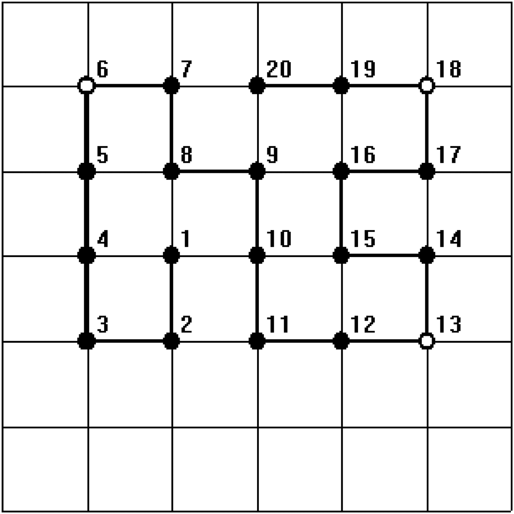
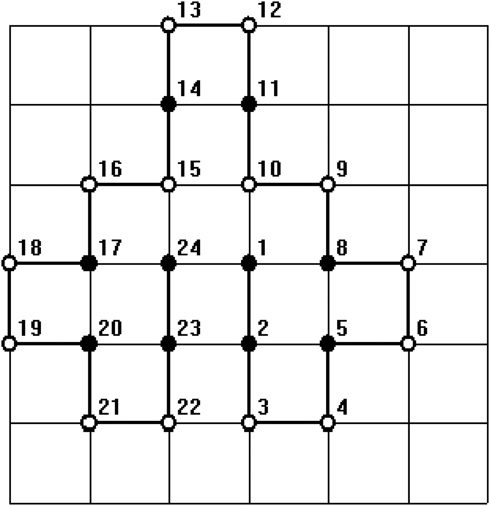
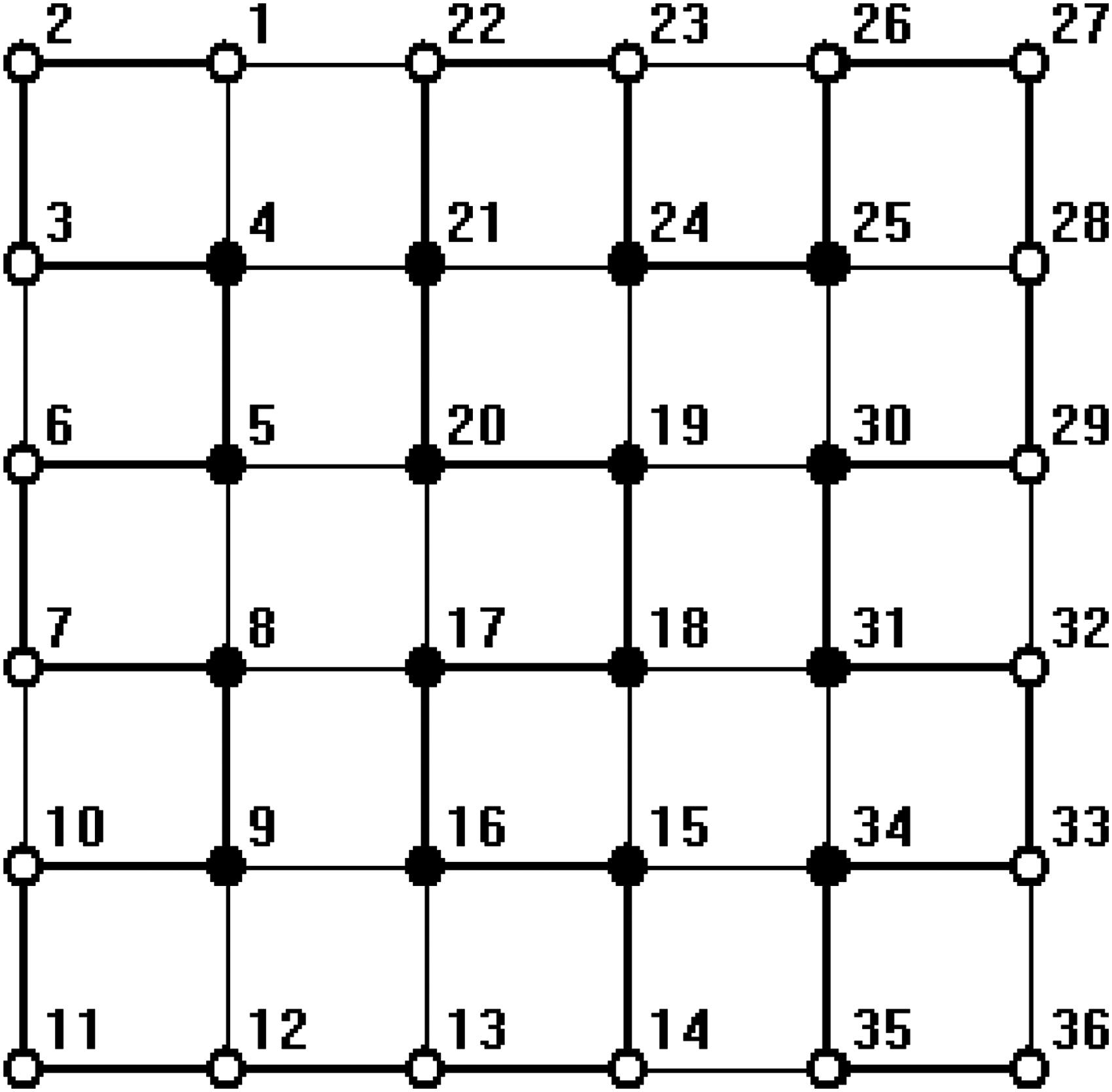
In all figures, hydrophobic will be depicted as “•” and hydrophilic as “ ∘ .” The bold line represents the covalent bond between adjacent amino acids, and the light line is the edge of the lattice.
For the sequence with length 20, HHHHHPHHHHHHPHHHHPHH, which comes from Zhang et al., 2005), we embedded the HP sequence into the 7 × 7 lattice. We find all the corresponding native structures listed two brand new conformations as shown in Figures 1 and 2. Due to the bigger lattice with more free space, new structures can be generated. The results of the experiment demonstrate that the proposed algorithm has the ability to search a complete set of optimal solutions.
One of the minimum energy configurations of the sequence length 20 by our method.
One of the minimum energy configurations of the sequence length 20 by our method.
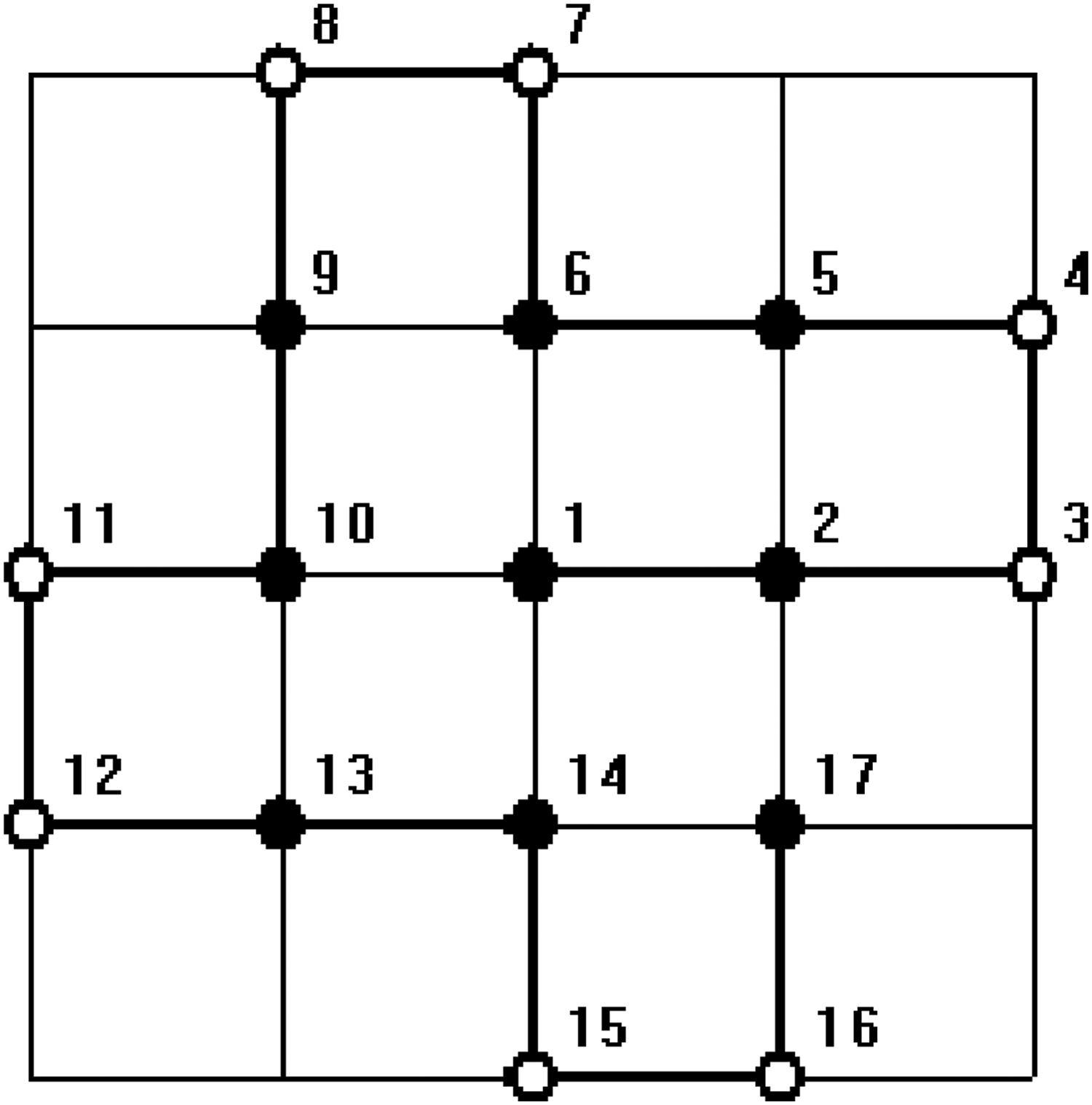
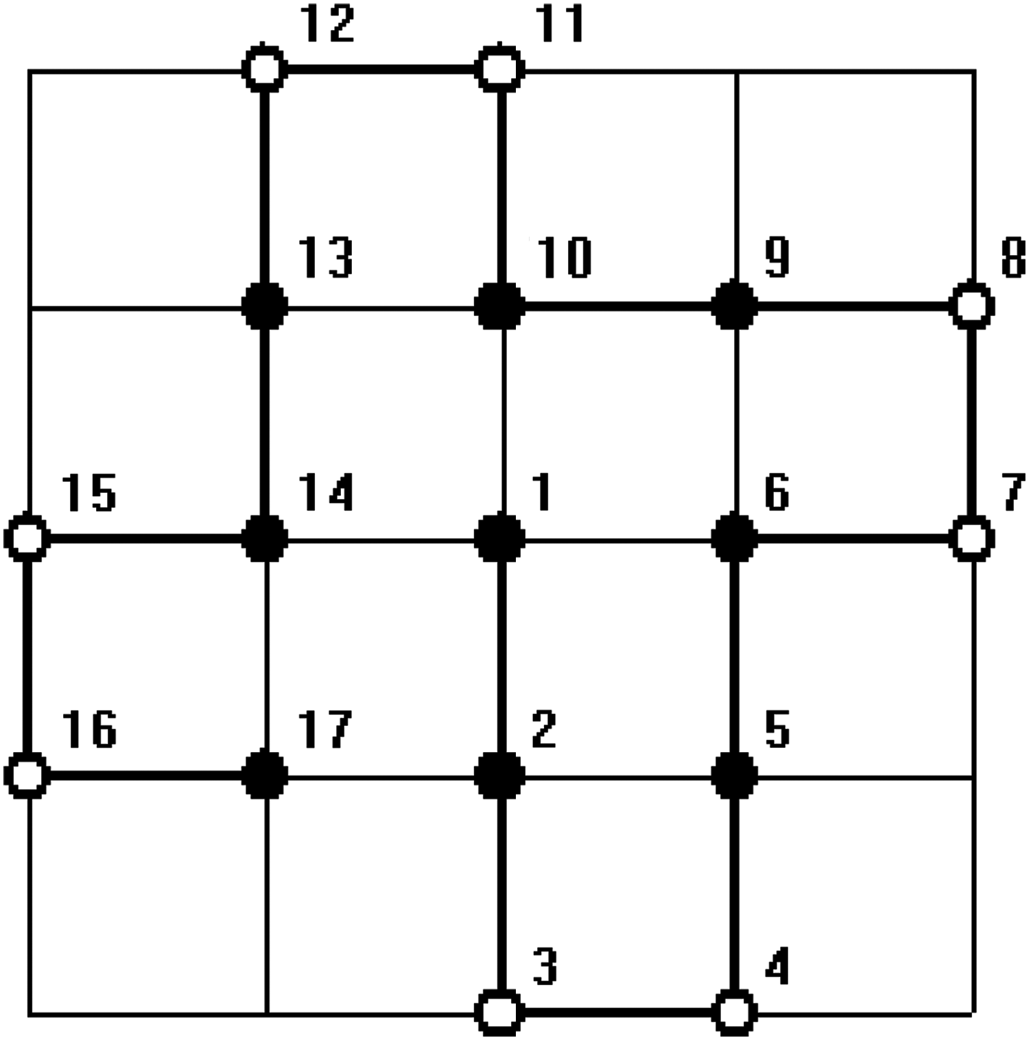
In order to test the ability of the proposed algorithm to deal with arbitrary length sequence, that is, the length n is not necessarily to be the product of two integers p and q, an HP sequence with length 17, HHPPHHPPHHPPHHPPH (Zhang et al., 2005), was computed. The results in a nonrectangular structure are constructed. Since this sequence can not be put into a regular lattice, it is beyond the ability of the conventional algorithms. It can be proved that the optimal structure of this sequence is unique regardless of symmetric transformation. The results of numerical simulation are given in Figures 3 and 4.
One of the minimum energy configurations of the sequence length 17 by our method.
One of the minimum energy configurations of the sequence length 17 by our method.
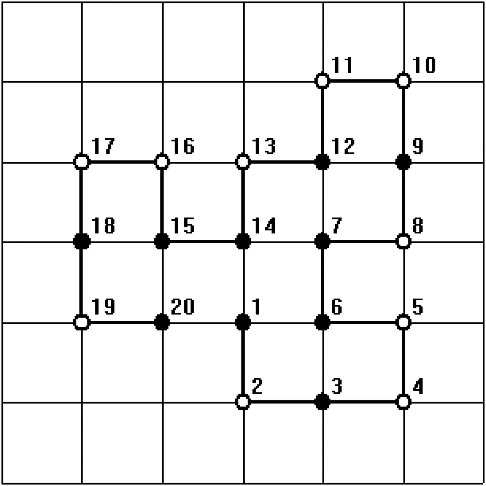
Some sequences of the HP benchmark (William and Sorin) were tested using our method. In all test sequences up to 48 amino acids, the proposed method is able to find the global optimal conformations of them. Three native structures of them are illustrated in Figures 5–7. We embedded the HP sequence of length 20, HPHPPHHPHPPHPHHPPHPH, into the 7 × 7 lattice; the HP sequence of length 48, PPHPPHHPPHHPPPPPHHHHHHHHHHPPPPPPHHPPHHPPHPPHHHHH, into the 9 × 9 lattice; and the HP sequence of length 24, HHPPHPPHPPHPPHPPHPPHPPHH, into the 7 × 7 lattice. All native structures are nonrectangle in structure. These results demonstrate that the protein shapes are not limited by the lattice.
The minimum energy configuration of the sequence length 20 by the proposed method.
The minimum energy configuration of the sequence length 24 by the proposed method.
The minimum energy configuration of the sequence length 48 by our proposed method
For some sequences in the HP benchmark that the chain can be compactly embedded to a regular lattice by other methods (Yanikoglu and Erman, 2002), our algorithm can also be simplified to solve these problems. For example, the sequence of length 36, PPPHHPPHHPPPPPHHHHHHHPPHHPPPPHHPPHPP, can be embedded into 6 × 6 lattice, and the sequence of length 25, PPHPPHHPPPPHHPPPPHHPPPPHH, can be embedded into 5 × 5 lattice. The minimum energy configurations are shown in Figures 8 and 9.
The minimum energy configuration of the sequence length 36 by our proposed method.
The minimum energy configuration of the sequence length 25 by our proposed method.
The results show that our algorithm for the 2D HP lattice model has four advantages: the ability to search a complete set of optimal solution; the ability to handle arbitrary length protein; the ability to obtain protein shape without limitation; and the ability to solve special sequences.
Compared with other methods used to solve the protein folding problem, the proposed algorithm is better and faster. The modified EN method has the advantage of being easily parallelizable by Equation (6). The weight values are adjusted so that some constraints are satisfied rapidly, so computing time is saved.
5. Discussion and Conclusions
In this article, we show how the modified elastic net algorithm is used as an efficient tool to solve the two-dimensional HP model. By putting the chain into a bigger lattice, the global minimum configuration of the amino acid chain is no longer compactly limited in a squarelike or other specific-shaped lattice. In other words, the protein sequence in the proposed model may have more free space to fold into the native structure with a lower energy value, and the length of the sequence is not limited to the product of two integers. Weight adjusted strategies and local search methods I and II are developed to overcome the difficulties brought by the bigger lattice. The proposed method is still time-consuming for large-scale folding problems, so how to make it more efficient is one of the directions for further research. As the recent research work indicated, the HP model is very useful for modeling protein properties, although it is simple and abstractive with several disadvantages. Recently, HP model has been applied to the investigation of aspects of ligand binding to protein (Miller and Dill, 1997), and in the work by Makovets and Blackburn (Makovets and Blackburn, 2009).
In future work, we intend to develop and study the EN algorithm, local search methods, weight adjusted strategy, and lattice partition strategy for other types of protein folding problems such as 3D compact HP lattice model, 2D triangular lattice model, 3D triangular lattice model, 2D diamond lattice model, and others. In addition, we will analyze the designability of protein structure and compute the complexity of computation of our algorithm. Overall, we strongly believe that our method offers considerable potential for solving protein structure prediction problems robustly and efficiently and that future work in this area should be undertaken.
Footnotes
Acknowledgments
This work is supported by subject of Foundation of China (Grant No. NN2014083).
References
1.
AlenaS., RosaliaA.H., and HolgerH.H.2005. An ant colony optimization algorithm for the 2D HP protein folding problem. Ant Algor. 2463, 40–53.
2.
BallK.D., ErmanB., and DillK.A.2002. The elastic net algorithm and protein structure prediction. J. Comp. Chem. 23, 77–83.
3.
CustódioF.L., BarbosaH.J.C., and DardenneL.E.2004. Investigation of the three-dimensional lattice HP protein folding model using a genetic algorithm. Genet. Mol. Biol., 27, 611–615.
4.
DillK.A., BrombergS., YueK., et al.1995. Principles of protein folding—a perspective from simple exact models. Protein Sci. 4, 561–602.
5.
DurbinR., and WillshawD.1987. An analogue approach to the travelling salesman problem using an elastic net method. Nature. 326, 689–691.
6.
GuoY.Z., FengE.M., ZhaoJ.C., et al.2007. Optimal HP configurations of protein by combining local search with elastic net algorithm. J. Biochem. Biophys. Method, 70, 335–340.
7.
HopfieldJ.J., and TankD.W.1985. Neural computation of decisions in optimization problems. Biol. Cybernet. 52, 141–152.
8.
JiangT.Z., CuiQ.H., ShiG.H., et al.2003. Protein folding simulations of the hydrophilic model by combining tabu search with genetic algorithms. J. Chem. Phys. 119, 4592–4596.
9.
LauK.F., and DillK.A.1998. A lattice statistical mechonics model of the conformation and sequence space of proteins. Macromolecules. 22, 3986–3997.
10.
LiangF.M., and WongW.H.2001. Evolutionary Monte Carlo for protein folding simulations. J. Chem. Phys. 115, 3374–3380.
11.
MakovetsS., and BlackburnE.H.2009. DNA damage signalling prevents deleterious telomere addition at DNA breaks. Nat. Cell. Biol., 11, 1383–1386.
12.
MillerD.W., and DillK.A.1997. Ligand binding to proteins: the binding landscape model. Protein Sci. 6, 2166–2179.
13.
SailA., ShakhnovichE.I., and KarplusM.1994. How does a protein fold?. Neture, 369, 248–251.
14.
SimicP.D.1991. Constrained nets for graph matching and other quadratic assigment problem. Neural Comp. 3, 268–281.
15.
UngerR., and MoultJ.1993. Genetic algorithms for protein folding simulations. J. Mol. Biol. 231, 75–81.
YanikogluB., and ErmanB.2002. Minimum energy configuration of the 2-dimensional HP-model of proteins by self-organizing networks. J. Comp. Biol. 9, 613–620.
18.
ZhangX.S., WangY., ZhanZ.W., et al.2005. Exploring protein's optimal HP congfigurations by self-organizing. J. Bioinform. Comput. Biol. 3, 385–400.