A Probabilistic Model of Neutral and Selective Dynamics of Protein Network Evolution

Abstract

Comparative approaches in genomics have long relied on rigorous mathematical models of sequence evolution. Such models provide the basis for formulating and solving well-defined computational problems, in turn yielding key insights into the evolutionary processes acting on the genome. Analogous model-based approaches for analyzing biological networks are still under development. Here we describe a model-based approach for estimating the probability of network rewiring events during evolution. Our method builds on the standard duplication-and-divergence model and incorporates phylogenetic analysis to guide the comparison of protein networks across species. We apply our algorithm to study the evolution of functional modules and unconstrained network regions in seven available eukaryotic interactomes. Based on this analysis we identify a map of co-functioning protein families whose members participate in strongly conserved interactions and form major complexes and pathways in the eukaryotic cell. The proposed approach provides principled means for inferring the probability of network rewiring events, enabling insights into the conservation and divergence of protein interactions and the formation of functional modules in protein networks.

1. Introduction

After a decade of large-scale screening, vast amounts of protein–protein interaction (PPI) data have been collected for a number of organisms. Although far from being complete, the available partial interactomes are routinely used as a system-level framework for interrogating cellular processes and conditions (Dutkowski and Ideker, 2011). Some of the most successful investigations have identified evolutionary conserved subnetworks in multiple distantly related organisms, enabling inferences about essential network connections and providing hypotheses on novel functional units (reviewed in Sharan and Ideker, 2006). Independently from these studies, theoretical models have been constructed providing insights into network phenomena such as the scale-free degree distribution (Barabási and Albert, 1999), high degree of clustering (Watts and Strogatz, 1998), and emergence of functional modules (Pereira-Leal et al., 2007).

Existing approaches for comparing networks across species differ substantially both in terms of mathematical formulations of the problem as well as applied algorithms. Early procedures searching for local subnetworks conserved across two species (Kelley et al., 2003; Sharan et al., 2005a; Koyuturk et al., 2006) have been complemented by multiple network aligners (Sharan et al., 2005b; Flannick et al., 2006). Global alignment has been formulated and solved by integer quadratic programming (Li et al., 2007). New graph-theoretic algorithms (Narayanan and Karp, 2007; Kalaev et al., 2009) and spectral approaches inspired by Google's page-rank algorithm have been proposed (Singh et al., 2007; Liao et al., 2009). Available methods offer a diverse range of scoring functions, including those motivated by evolutionary considerations (Koyuturk et al., 2006; Hirsh and Sharan, 2006; Berg and Lassig, 2006; Flannick et al., 2008), as well as structural and functional similarity (Kuchaiev and Pržulj, 2011; Ali and Deane, 2009).

Apart from developments in network alignment, multiple studies have focused on constructing and analyzing random graph models that aim to capture the basic processes by which protein networks evolve. Most of these models are based on the principle of duplication and divergence (Sole et al., 2002; Vazquez et al., 2003; Bebek et al., 2005; Berg et al., 2004; Ispolatov et al., 2005b; Ispolatov et al., 2005a; Evlampiev and Isambert, 2008) and have shown to match the observed data in terms of key topological features such as degree distribution and clustering coefficient (Bebek et al., 2006; Hormozdiari et al., 2007). When these models are fitted to experimental data, they provide important insights about the evolutionary forces shaping the network topology. Functional inferences, however, are challenging because nodes in these network models are typically anonymous and cannot be mapped to specific genes or proteins in the real networks. Additionally, these models typically describe the network of a single organism. Hence, although very interesting insights have been made using traditional random graph models, for example, recent inferences of putative ancestral network states (Navlakha and Kingsford, 2011), their ability to jointly model network evolution across species remains limited (Knight and Pinney, 2009).

To provide a model-based approach for comparing networks across species, we have previously developed conserved ancestral protein-protein interactions (CAPPI) (Dutkowski and Tiuryn, 2007), which applies phylogenetic analysis to reconstruct the history of protein sequence evolution based on which it further infers the evolution of protein interactions. CAPPI applies a model closely resembling the random graph models previously proposed, but it additionally adds a speciation event—a natural extension that allows us to consider networks from multiple species. The second crucial difference compared to standard random graph models is that the duplication and speciation events are linked directly to the specific proteins in the underlying biological networks, allowing for functional analysis of real networks. Originally, CAPPI was designed to perform local network alignment, that is, to identify conserved network regions under a user-specified model. It was further extended to handle missing links in networks and predict new protein interactions (Dutkowski and Tiuryn, 2009).

In the present work we take a new direction. First, we develop an expectation-maximization (Dempster et al., 1977) algorithm to learn the parameters of the evolutionary model automatically from experimental data, providing the first cross-species estimations of PPI evolutionary rates under a duplication-and-divergence model. This approach significantly extends CAPPI's network modeling capabilities, allowing for direct estimation of evolutionary parameters, parameter-free identification of conserved network regions, and reconstruction of ancestral and consensus network representations for multiple species. Next, we introduce two instances of the model: one that corresponds to evolution under selective pressure, and the other one that fits the neutral scenario. We train the two models on specific examples of known functional modules and randomly selected network regions. Finally, for every pair of protein families, we compute the likelihood of evolving under the conserved and under the random model. Using this method, we infer the most conserved network regions across seven eukaryotic species and identify cofunctioning protein families whose members participate in major eukaryotic complexes and pathways.

2. Methods

We first briefly summarize the network model (Dutkowski and Tiuryn, 2009) and then present the expectation maximization (EM) algorithm developed in the present study.

2.1. The model of PPI network evolution

Suppose we have a set of protein–protein interaction networks for several species. We first construct a phylogenetic tree for the input species and cluster all protein sequences present in these species to define clusters of paralogous proteins. Each cluster, also called a protein family, corresponds to a single protein in the ancestral species. Each family gives rise to a reconciled phylogenetic tree (Page and Charleston, 1997), which, in addition to speciation, uses duplication events and gene losses to explain the particular protein composition of the family. The reconciled trees are constructed subject to minimization of the number of duplication and loss events.

Assume real-valued parameters Θ = (p_s, δ_s, p_d, δ_d, p_m, δ_m, p_*) and an initial network of protein–protein interactions represented by an undirected graph G. The graph G can be thought of as an ancestral network of interactions, where nodes correspond to the proteins and edges connect two interacting partners. The parameter p_* represents the (prior) probability of observing an edge in G. The network evolves subject to the following events:

• Speciation gives rise to two graphs (for two species) in which edges are retained with probability p_s and new (non-existing) edges are introduced with probability δ_s.

• Duplication gives rise to a new graph, which is obtained from the predecessor by duplicating one of its nodes. Edges incident to the node that was duplicated are retained with probability p_d, and new edges incident to this node are introduced with probability δ_d. This is done independently for each of the two duplicated nodes.

• Measurement (this is the addition to the original model of Dutkowski and Tiuryn, 2007). With this event, we model the possibility of introducing errors during the measurement process. The resulting graph represents the input dataset. Each edge is retained with probability p_m, and new (non-existing) edges are introduced with probability δ_m. The reader may have noticed that this step is similar to the speciation event, except that there is only one successor instead of two. Actually this part of the model can be further refined by introducing separate parameters for different input sets, addressing in this way specific reliability of the data.

The above speciation and duplication events can be naturally associated with corresponding events in the reconciled phylogenetic trees, thus representing the evolution of interactions spanning every pair of protein families (for details see Dutkowski and Tiuryn, 2007, 2009).

2.2. EM parameter estimation

Based on this model, we now develop an EM approach for deriving the probabilities of network rewiring events directly from the existing interaction data. We have two types of such events associated with speciation: retaining an edge and introducing an edge. We denote these two types by s and s⁺, respectively. In a similar fashion we define the events d, d⁺, m, m⁺. We introduce the concept of an event in order to easily refer in a uniform way to the corresponding parameters of the model. For this reason, we will also include the event of initiation and denote it by*. This event represents creation of the ancestral graph G by a sequence of edge introductions. Let E = {s, s⁺, d, d⁺, m, m⁺, *} denote the set of all types of events. With each type e ∈ E there is naturally associated a probability p_e for this event to occur. Thus, for example, p_s retains its meaning from the parameter set Θ, and \documentclass{aastex}\usepackage{amsbsy}\usepackage{amsfonts}\usepackage{amssymb}\usepackage{bm}\usepackage{mathrsfs}\usepackage{pifont}\usepackage{stmaryrd}\usepackage{textcomp}\usepackage{portland, xspace}\usepackage{amsmath, amsxtra}\pagestyle{empty}\DeclareMathSizes {10} {9} {7} {6} \begin{document} $$p_{d^ + } = \delta_d$$ \end{document} . We will write p_e_,Θ if we want to make explicit dependence on the parameter set Θ. For each type e, by ¬e we denote the complementary event. Hence, for example, ¬d denotes the event of loosing an edge, while ¬m⁺ denotes the event of not introducing an edge that was not previously present. Clearly we have p_¬e = 1 − p_e.

Our model consists of two levels: the observable level, which is represented by datasets of measured protein–protein interactions, and the hidden level that represents the true extant interactions together with all protein interactions that were present during the evolution from the ancestral species to the extant species. The speciation and duplication events are internal in the hidden level, while the measurement event serves as a bridge between the hidden and the observable levels.

Let us denote by \documentclass{aastex}\usepackage{amsbsy}\usepackage{amsfonts}\usepackage{amssymb}\usepackage{bm}\usepackage{mathrsfs}\usepackage{pifont}\usepackage{stmaryrd}\usepackage{textcomp}\usepackage{portland, xspace}\usepackage{amsmath, amsxtra}\pagestyle{empty}\DeclareMathSizes {10} {9} {7} {6} \begin{document} $${ \cal X}$$ \end{document} the set of all possible states of experimental outcomes and by \documentclass{aastex}\usepackage{amsbsy}\usepackage{amsfonts}\usepackage{amssymb}\usepackage{bm}\usepackage{mathrsfs}\usepackage{pifont}\usepackage{stmaryrd}\usepackage{textcomp}\usepackage{portland, xspace}\usepackage{amsmath, amsxtra}\pagestyle{empty}\DeclareMathSizes {10} {9} {7} {6} \begin{document} $${ \bf x} = ( x_1 , \ldots , x_n ) \in { \cal X}$$ \end{document} the particular instance observed in the data, where x_i is equal to 1 when the i-th experimental reading (a particular experimental observation for a given protein pair) was positive and 0 otherwise. Similarly denote by \documentclass{aastex}\usepackage{amsbsy}\usepackage{amsfonts}\usepackage{amssymb}\usepackage{bm}\usepackage{mathrsfs}\usepackage{pifont}\usepackage{stmaryrd}\usepackage{textcomp}\usepackage{portland, xspace}\usepackage{amsmath, amsxtra}\pagestyle{empty}\DeclareMathSizes {10} {9} {7} {6} \begin{document} $${ \bf y} = ( y_1 , \ldots , y_m ) \in { \cal Y}$$ \end{document} one particular instance of all hidden interactions chosen from the set \documentclass{aastex}\usepackage{amsbsy}\usepackage{amsfonts}\usepackage{amssymb}\usepackage{bm}\usepackage{mathrsfs}\usepackage{pifont}\usepackage{stmaryrd}\usepackage{textcomp}\usepackage{portland, xspace}\usepackage{amsmath, amsxtra}\pagestyle{empty}\DeclareMathSizes {10} {9} {7} {6} \begin{document} $${ \cal Y}$$ \end{document} of all possible states of these random variables. In this case y_i equals 1 if the i-th pair of proteins interact with each other and 0 otherwise. Observe that information about the states x and y uniquely describes all graphs of interactions between proteins in extant as well as ancestral species.

For a type \documentclass{aastex}\usepackage{amsbsy}\usepackage{amsfonts}\usepackage{amssymb}\usepackage{bm}\usepackage{mathrsfs}\usepackage{pifont}\usepackage{stmaryrd}\usepackage{textcomp}\usepackage{portland, xspace}\usepackage{amsmath, amsxtra}\pagestyle{empty}\DeclareMathSizes {10} {9} {7} {6} \begin{document} $$e \in E$$ \end{document} and for a state of the hidden variables y, we denote by A_e(y) the number of events of type e in the model defined by y (and x). We assume that x is known, and therefore, we do not write the explicit dependence of A_e(y) on it. In a similar way we define A_¬e(y).

2.2.1. The \documentclass{aastex}\usepackage{amsbsy}\usepackage{amsfonts}\usepackage{amssymb}\usepackage{bm}\usepackage{mathrsfs}\usepackage{pifont}\usepackage{stmaryrd}\usepackage{textcomp}\usepackage{portland, xspace}\usepackage{amsmath, amsxtra}\pagestyle{empty}\DeclareMathSizes {10} {9} {7} {6} \begin{document} $${ \cal Q}$$ \end{document} function

We now derive the \documentclass{aastex}\usepackage{amsbsy}\usepackage{amsfonts}\usepackage{amssymb}\usepackage{bm}\usepackage{mathrsfs}\usepackage{pifont}\usepackage{stmaryrd}\usepackage{textcomp}\usepackage{portland, xspace}\usepackage{amsmath, amsxtra}\pagestyle{empty}\DeclareMathSizes {10} {9} {7} {6} \begin{document} $${ \cal Q}$$ \end{document} function for our model. For two parameter sets Θ and Θ^t we define \documentclass{aastex}\usepackage{amsbsy}\usepackage{amsfonts}\usepackage{amssymb}\usepackage{bm}\usepackage{mathrsfs}\usepackage{pifont}\usepackage{stmaryrd}\usepackage{textcomp}\usepackage{portland,xspace}\usepackage{amsmath,amsxtra}\pagestyle{empty}\DeclareMathSizes{10}{9}{7}{6} \begin{document} \begin{align*}{ \cal Q} ( \Theta \mid \Theta^t ) = \sum_{ \bf y} P ( { \bf y} \mid { \bf x} , \Theta^t ) \log P ( { \bf x} , { \bf y} \mid \Theta ) . \tag{1}\end{align*} \end{document}

The probability of the data given the parameters Θ can be expressed as the product of the probabilities of the initial interactions and the transition probabilities: \documentclass{aastex}\usepackage{amsbsy}\usepackage{amsfonts}\usepackage{amssymb}\usepackage{bm}\usepackage{mathrsfs}\usepackage{pifont}\usepackage{stmaryrd}\usepackage{textcomp}\usepackage{portland,xspace}\usepackage{amsmath,amsxtra}\pagestyle{empty}\DeclareMathSizes{10}{9}{7}{6} \begin{document} \begin{align*}P ( { \bf x} , { \bf y} \mid \Theta ) = \prod_{e \in E} \left( p_{e , \Theta}^{A_e ( { \bf y} ) } \cdot ( 1 - p_{e , \Theta} ) ^{A_{ \neg e} ( { \bf y} ) } \right) .\end{align*} \end{document}

Applying usual transformations we obtain the following formula for \documentclass{aastex}\usepackage{amsbsy}\usepackage{amsfonts}\usepackage{amssymb}\usepackage{bm}\usepackage{mathrsfs}\usepackage{pifont}\usepackage{stmaryrd}\usepackage{textcomp}\usepackage{portland, xspace}\usepackage{amsmath, amsxtra}\pagestyle{empty}\DeclareMathSizes {10} {9} {7} {6} \begin{document} $${ \cal Q}$$ \end{document} \documentclass{aastex}\usepackage{amsbsy}\usepackage{amsfonts}\usepackage{amssymb}\usepackage{bm}\usepackage{mathrsfs}\usepackage{pifont}\usepackage{stmaryrd}\usepackage{textcomp}\usepackage{portland,xspace}\usepackage{amsmath,amsxtra}\pagestyle{empty}\DeclareMathSizes{10}{9}{7}{6} \begin{document} \begin{align*}{ \cal Q} ( \Theta \mid \Theta^t ) = \sum_e \left( {\mathbb E} ( A_e ) \log p_{e , \Theta} + {\mathbb E} ( A_{ \neg e} ) \log ( 1 - p_{e , \Theta} ) \right) , \tag{2}\end{align*} \end{document}

where the mean values are taken with respect to the probability distribution P(−|x, Θ^t). The details of these transformations are given in the Supplementary Material (available online at www.liebertonline.com/cmb).

2.2.2. The E-step

In the E-step we compute the mean values \documentclass{aastex}\usepackage{amsbsy}\usepackage{amsfonts}\usepackage{amssymb}\usepackage{bm}\usepackage{mathrsfs}\usepackage{pifont}\usepackage{stmaryrd}\usepackage{textcomp}\usepackage{portland, xspace}\usepackage{amsmath, amsxtra}\pagestyle{empty}\DeclareMathSizes {10} {9} {7} {6} \begin{document} $${\mathbb E} ( A_e )$$ \end{document} and \documentclass{aastex}\usepackage{amsbsy}\usepackage{amsfonts}\usepackage{amssymb}\usepackage{bm}\usepackage{mathrsfs}\usepackage{pifont}\usepackage{stmaryrd}\usepackage{textcomp}\usepackage{portland, xspace}\usepackage{amsmath, amsxtra}\pagestyle{empty}\DeclareMathSizes {10} {9} {7} {6} \begin{document} $${\mathbb E} ( A_{ \neg e} )$$ \end{document} , with e ranging over all types. The mean values are taken with respect to the probability distribution P(−|x, Θ^t). They are computed using Pearl's message-passing algorithm. Again the details are given in the Supplementary Material.

2.2.3. The M-step

The M-step of the algorithm determines new parameter values that maximize the \documentclass{aastex}\usepackage{amsbsy}\usepackage{amsfonts}\usepackage{amssymb}\usepackage{bm}\usepackage{mathrsfs}\usepackage{pifont}\usepackage{stmaryrd}\usepackage{textcomp}\usepackage{portland, xspace}\usepackage{amsmath, amsxtra}\pagestyle{empty}\DeclareMathSizes {10} {9} {7} {6} \begin{document} $${ \cal Q}$$ \end{document} function. The terms of the expression (2) can be maximized separately with respect to one of the model parameters: \documentclass{aastex}\usepackage{amsbsy}\usepackage{amsfonts}\usepackage{amssymb}\usepackage{bm}\usepackage{mathrsfs}\usepackage{pifont}\usepackage{stmaryrd}\usepackage{textcomp}\usepackage{portland,xspace}\usepackage{amsmath,amsxtra}\pagestyle{empty}\DeclareMathSizes{10}{9}{7}{6} \begin{document} \begin{align*}{\mathbb E} ( A_e ( { \bf y} ) ) \log (\, p_e ) + {\mathbb E} ( A_{ \neg e} ( { \bf y} ) ) \log ( 1 - p_e ) , \hbox{for each type} \ e.\end{align*} \end{document}

For a given e, we find \documentclass{aastex}\usepackage{amsbsy}\usepackage{amsfonts}\usepackage{amssymb}\usepackage{bm}\usepackage{mathrsfs}\usepackage{pifont}\usepackage{stmaryrd}\usepackage{textcomp}\usepackage{portland, xspace}\usepackage{amsmath, amsxtra}\pagestyle{empty}\DeclareMathSizes {10} {9} {7} {6} \begin{document} $$p_e^*$$ \end{document} for which the derivative is equal to 0: \documentclass{aastex}\usepackage{amsbsy}\usepackage{amsfonts}\usepackage{amssymb}\usepackage{bm}\usepackage{mathrsfs}\usepackage{pifont}\usepackage{stmaryrd}\usepackage{textcomp}\usepackage{portland,xspace}\usepackage{amsmath,amsxtra}\pagestyle{empty}\DeclareMathSizes{10}{9}{7}{6} \begin{document} \begin{align*} & \frac { \partial { \cal Q } } { \partial p_e } = \frac { { \mathbb E } ( A_e ) } { p_e^* } - \frac { { \mathbb E } ( A_ { \neg e } ) } { 1 - p_e^* } = 0 \\ & p_e^* = \frac { { \mathbb E } ( A_e ) } { { \mathbb E } ( A_e ) + { \mathbb E } ( A_ { \neg e } ) } . \end{align*} \end{document}

Notice that \documentclass{aastex}\usepackage{amsbsy}\usepackage{amsfonts}\usepackage{amssymb}\usepackage{bm}\usepackage{mathrsfs}\usepackage{pifont}\usepackage{stmaryrd}\usepackage{textcomp}\usepackage{portland, xspace}\usepackage{amsmath, amsxtra}\pagestyle{empty}\DeclareMathSizes {10} {9} {7} {6} \begin{document} $$ \frac { \partial { \cal Q } } { \partial p_e } > 0$$ \end{document} for \documentclass{aastex}\usepackage{amsbsy}\usepackage{amsfonts}\usepackage{amssymb}\usepackage{bm}\usepackage{mathrsfs}\usepackage{pifont}\usepackage{stmaryrd}\usepackage{textcomp}\usepackage{portland, xspace}\usepackage{amsmath, amsxtra}\pagestyle{empty}\DeclareMathSizes {10} {9} {7} {6} \begin{document} $$p_e < p_e^*$$ \end{document} and \documentclass{aastex}\usepackage{amsbsy}\usepackage{amsfonts}\usepackage{amssymb}\usepackage{bm}\usepackage{mathrsfs}\usepackage{pifont}\usepackage{stmaryrd}\usepackage{textcomp}\usepackage{portland, xspace}\usepackage{amsmath, amsxtra}\pagestyle{empty}\DeclareMathSizes {10} {9} {7} {6} \begin{document} $$ \frac { \partial { \cal Q } } { \partial p_e } < 0$$ \end{document} for \documentclass{aastex}\usepackage{amsbsy}\usepackage{amsfonts}\usepackage{amssymb}\usepackage{bm}\usepackage{mathrsfs}\usepackage{pifont}\usepackage{stmaryrd}\usepackage{textcomp}\usepackage{portland, xspace}\usepackage{amsmath, amsxtra}\pagestyle{empty}\DeclareMathSizes {10} {9} {7} {6} \begin{document} $$p_e > p_e^*$$ \end{document} . Thus \documentclass{aastex}\usepackage{amsbsy}\usepackage{amsfonts}\usepackage{amssymb}\usepackage{bm}\usepackage{mathrsfs}\usepackage{pifont}\usepackage{stmaryrd}\usepackage{textcomp}\usepackage{portland, xspace}\usepackage{amsmath, amsxtra}\pagestyle{empty}\DeclareMathSizes {10} {9} {7} {6} \begin{document} $$p_e^*$$ \end{document} is the optimal value and is selected as p_e in the new set of parameters Θ^t+1.

2.3. Discriminating between selective and neutral evolution

To learn the parameters associated with conserving and neutral network evolution, we use protein interactions among members of functional modules as training samples for the conserving model, and interactions in random network regions for the neutral model. We run the EM procedure separately to obtain these two sets of parameters. Afterward, the two estimated models can be used to discriminate between the conserving and neutral cases. For a given pair of protein families (f₁, f₂) we define the log-likelihood ratio (LLR score) as: \documentclass{aastex}\usepackage{amsbsy}\usepackage{amsfonts}\usepackage{amssymb}\usepackage{bm}\usepackage{mathrsfs}\usepackage{pifont}\usepackage{stmaryrd}\usepackage{textcomp}\usepackage{portland,xspace}\usepackage{amsmath,amsxtra}\pagestyle{empty}\DeclareMathSizes{10}{9}{7}{6} \begin{document} \begin{align*}LLR ( f_1 , f_2 ) = \log \frac { P ( { \bf x } _ { f_1 , f_2 } \mid \Theta_ { conserving } ) } { P ( { \bf x } _ { f_1 , f_2 } \mid \Theta_ { neutral } ) } ,\end{align*} \end{document}

where \documentclass{aastex}\usepackage{amsbsy}\usepackage{amsfonts}\usepackage{amssymb}\usepackage{bm}\usepackage{mathrsfs}\usepackage{pifont}\usepackage{stmaryrd}\usepackage{textcomp}\usepackage{portland, xspace}\usepackage{amsmath, amsxtra}\pagestyle{empty}\DeclareMathSizes {10} {9} {7} {6} \begin{document} $${ \bf x}_{f_1 , f_2}$$ \end{document} denotes all experimental readings for interactions between the members of families f₁ and f₂. The LLR is the logarithm of the ratio of the likelihood of the data under the model of conserving evolution and under the model of neutral evolution. If LLR>0 then the data are more likely under the conserving model.

3. Results and Discussion

We applied the proposed framework and reference datasets to estimate two types of parameters of network evolution (Fig. 1). The first type was estimated based on known examples of functional modules, which are assumed to evolve under a conserving evolutionary scenario. The second type was estimated based on randomly selected parts of the network. We expected that the difference between these parameter sets would reflect the difference in interaction conservation among functional modules and remaining network regions evolving at a background rate.

FIG. 1.

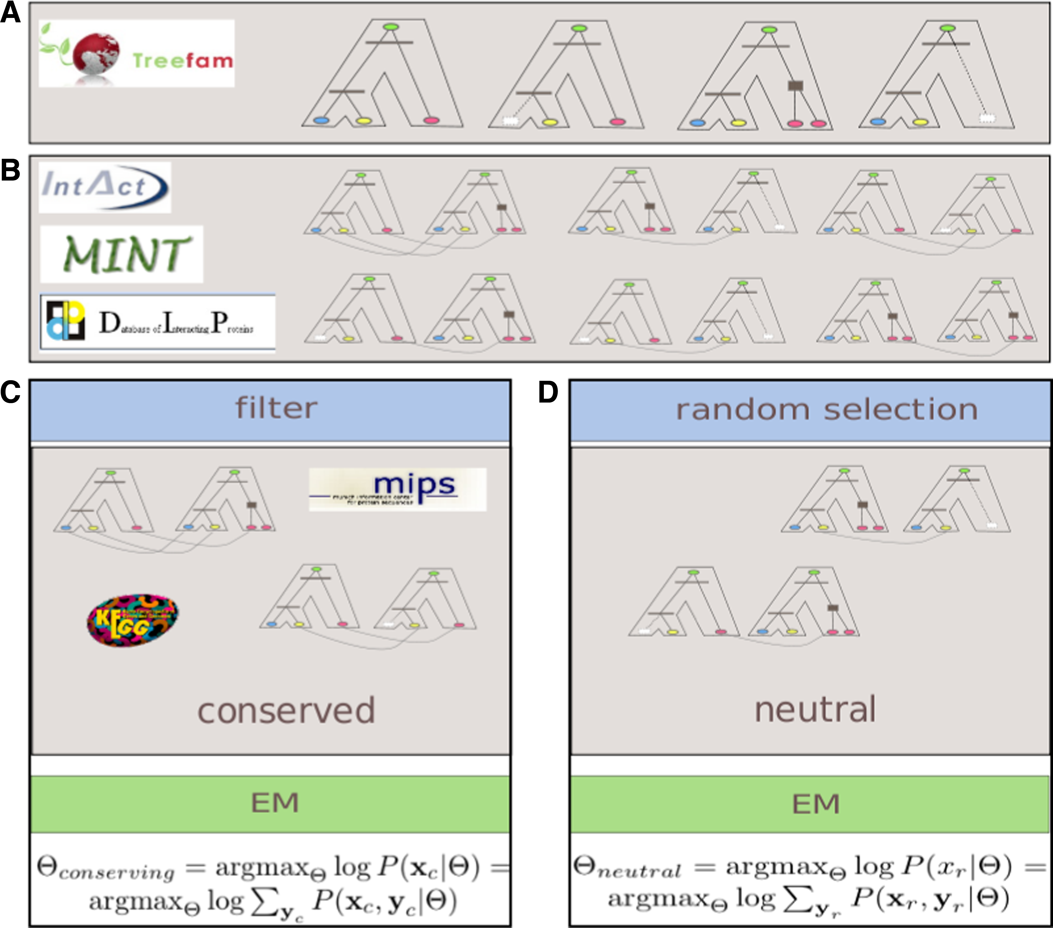
Estimating the parameters of conserving and neutral evolution of protein interaction networks: (A) Phylogenetic trees representing the evolution of specific protein families marked with duplication (filled box) and speciation (horizontal line) events are downloaded from the TreeFam database. The trees are pruned to consider only the seven species of interest. (B) Protein–protein interactions are downloaded from three major databases and are associated with the corresponding proteins in the leaves of the phylogenetic trees. Only pairs of trees for which there exist at least one interaction between member proteins are collected. (C) A filter is applied to the available pairs of trees to select for the conserved training set of pairs of families in which member proteins coexist either in the same KEGG pathway or a MIPS complex. (D) The second training set is comprised of an equal number of randomly selected pairs of trees. The model parameters for the conserving evolution scenario are estimated using the EM procedure based on the evidence from the conserved training set. The parameters for the neutral evolution scenario are derived based on evidence from the random set. Subsequently, the two estimated sets of model parameters are used to classify interactions between a new pair of protein families as either conserved or evolving under the neutral scenario.

3.1. Data acquisition

We downloaded the TreeFam database (Li et al., 2006) as a reliable source of protein families and phylogenies. TreeFam contained over 18,000 gene family trees of which 1,314 (in TreeFam A) were manually curated and are therefore attributed greater confidence. From TreeFam A we selected 573 families that have a representative from each of the seven species: H. sapiens, M. musculus, R. norvegicus, D. melanogaster, C. elegans, S. cerevisiae, and A. thaliana. Next we downloaded all available protein–protein interactions for these species from the IntAct (Hermjakob et al., 2004), DIP (Salwinski et al., 2004), and MINT (Chatr-aryamontri et al., 2007) databases.

Reference datasets of protein pathways and complexes were downloaded from the KEGG and MIPS databases. Based on the reference datasets we prepared two separate sets of examples of conserving PPI evolution. First for the KEGG-based dataset we extracted pairs of different yeast proteins that were together members of the same pathway. For each such pair of proteins, we added the corresponding pair of protein families (to which the proteins belonged to) to our set of conserved examples, but only if there was at least one protein–protein interaction observed between members of these families (in the input PPI databases). We refer to such family pairs as conserved. We identified 553 conserved pairs altogether. Analogous steps were performed for the MIPS dataset identifying 347 family pairs.

Next we generated a random dataset, equal in size to the larger of the two conserved sets, drawing only pairs of protein families for which there was at least one interaction observed between their members. Thus both the conserved and the random set contained pairs of protein families for which some evidence for interaction existed. Pairs in the conserved sets fulfill an additional condition—each family in the pair has at least one protein member in the same KEGG pathway or MIPS complex. Note that in both cases a protein family is allowed to form a pair with itself.

3.2. Parameter estimation

Next we estimated the parameters of the evolutionary model (p_s, δ_s, p_d, δ_d, p_*) based on the three training datasets (KEGG-based, MIPS-based, and random). Table 1 shows important differences between the three resulting models. Most notable is the conservation of interactions during speciation (p_s), which is greater for the conserved KEGG and MIPS-based models than for the random model. This result supports the notion that interactions within functional modules are strongly conserved across species. Perhaps less expected is the weaker conservation of these interactions during duplication (p_d). One plausible explanation is that it allows duplicate members of the functional modules to change function more easily. While the conservation of essential interactions is critical, once a protein duplicates one of the copies may be allowed to diverge and gain new functionality. This provides potential for higher interaction loss as well as for formation of new interactions by adapting old interfaces. It is also interesting to observe that parameter values estimated based on the MIPS data are more extreme than those based on KEGG. This suggests that interactions within complexes are more strongly conserved that those within pathways that generally define broader functional categories (often composed of several complexes).

Table 1.

Parameter Estimates Obtained for Three Different Training Datasets (Random, KEGG, and MIPS) Using the EM Procedure

Data	p_s	δ_s	p_d	δ_d	p_^*
Random	0.85	0.02	0.59	0.001	1 - (4.8e-06)
KEGG	0.93	0.04	0.55	3.1e-6	1 - (2.2e-16)
MIPS	0.98	0.05	0.49	3.8e-5	1 - (1.1e-16)

Finally, we notice that in all three models the prior probability of interaction is close to one, suggesting that the vast majority of present interactions have their evolutionary predecessors in the ancestral species. Note that based on the present day interactomes, the overall prior probability of interaction between ancestral proteins is expected to be ∼0.001. Here however, we only consider a specific subspace of the interactome defined by pairs of protein families for which at least one interaction is observed experimentally.

3.3. Distinguishing conserved pathway and complex regions

The differences between the models (conserving and neutral) enable us to apply the likelihood ratio score to assess the relative interaction conservation between members of arbitrary protein families. First, we analyze the scores among pairs of families used for training the two conserving models. The distribution of LLR scores for pairs of families derived based on KEGG and MIPS data are plotted in Figure 2. For KEGG-based pairs, the conserving model used to calculate the LLR scores was based on the KEGG database. The MIPS-based pairs were scored using the MIPS-based conserving model. Additionally, each pair was scored in the neutral model. As expected, in both cases most KEGG and MIPS-based pairs scored higher under the conserving model (LLR>0). However, we also identified a considerable fraction of pairs that were more likely under the neutral scenario (255 KEGG- and 140 MIPS-based pairs). The histograms (see Fig. 2 A, B) suggest a bimodal distribution where some of the KEGG- and MIPS-based family pairs are significantly more conserved than others. Based on this observation, we selected a stringent LLR threshold value, at which other highly conserved pairs can be identified. Figure 2 provides an overview of the top-scoring KEGG-based associations with LLR>0.2 grouped according to the KEGG pathways that support them. Among the most conserved pathway regions, we identified those involved in proteolysis, cell cycle, metabolism, and DNA replication.

FIG. 2.

Histograms provide the distribution of log-likelihood ratio (LLR) scores among pairs of protein families containing proteins belonging to common KEGG pathways (A) or MIPS complexes (B). (C) A pathway view of the top-scoring family associations (KEGG ID and description are given). Nodes correspond to protein families. Edges denote conservation of protein interactions between two families with LLR >0.2. The edges backed only by KEGG evidence are colored yellow. Those additionally supported by MIPS complexes are green.

3.4. Maps of highly conserved associations

Next we computed the LLR score for all remaining pairs of protein families using the MIPS-based conserving model and the neutral model. Further, we constructed a network of protein families in which the edges are weighted by the LLR score, representing the level of conservation of interactions between the members of adjacent families. Based on the considerations outlined above, we selected a threshold value of 0.4 and retained only the edges in the network with weights above this threshold. Family pairs with no edges above the selected threshold were discarded. Overall 251 protein families and 358 edges were retained.

The resulting network is visualized in Figure 3 (a high-resolution version is also available as Supplementary Fig. 1). The network has a giant component composed of 192 nodes and 316 edges. Additionally there are 29 considerably smaller components. Approximately half of the edges in the network correspond to protein family pairs, which were previously known to be associated within functional modules. In total, 105 of these correspond to pairs present in the MIPS-based dataset used for training. An additional 38 pairs (marked by yellow edges) are present only in the KEGG-based dataset—these were not present in the training set. The remaining 173 edges represent predicted novel family associations.

FIG. 3.

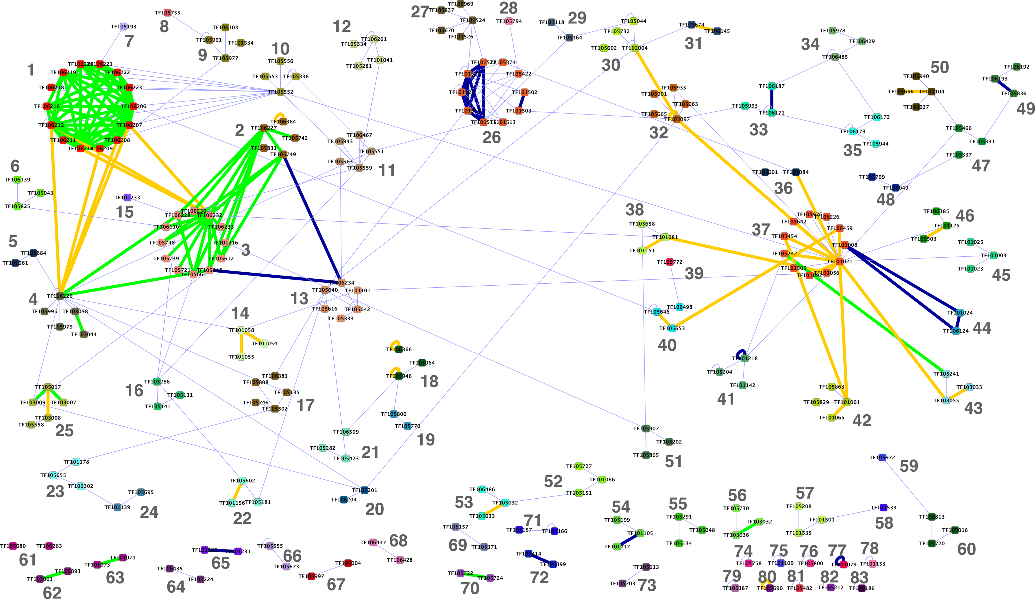
TreeFam family network identified at LLR threshold of 0.4 and clustered using the affinity propagation algorithm. Identified clusters are numbered and color coded. Thick edges correspond to known associations either based on MIPS (blue), KEGG (yellow), or both (green).

We further raised the LLR threshold value to identify multiple coherent network modules. Table 2 presents the results of gene ontology (GO) enrichment analysis (Bauer et al., 2008) of the 26 connected components of the family network identified as LLR = 0.7 (components are presented in Supplementary Fig. 2). We find that 24 of the 26 modules are significantly enriched for a biological process term (p-value <0.01 after correcting for multiple testing). The first two modules correspond to the proteasome complex involved in proteolysis (see above). Other modules are responsible for highly conserved biological processes such as translation, cell cycle regulation, protein folding, and phosphorylation. Most of the modules have enriched annotations to the same term in multiple species. Our analysis also uncovers possible missing annotations (denoted by NA in Table 2) and suggests candidate GO terms for the corresponding proteins. For example, based on the evidence from four other species, Arabidopsis proteins in component number 20 might be considered for annotation to the cell division term, while rat proteins belonging to the 7-th module are suspected to take part in DNA replication.

Table 2.

GO Term Enrichment Among the Connected Components of the Protein Family Network (Identified at LLR >0.7)

ID	Description	Arabidopsis	Yeast	Rat	Mouse	Human
1	Ubiquitin-dependent protein catabolic process	<0.0001	<0.0001	<0.0001	<0.0001	<0.0001
2	Protein catabolic process	<0.0001	<0.0001	0.0097	0.02	1.0E-4
3	Translation	<0.0001	1.0E-4	0.6338	<0.0001	<0.0001
4	Regulation of cell cycle	<0.0001	0.0080	4.0E-4	<0.0001	<0.0001
5	Phosphorylation	<0.0001	1	0.9318	2.0E-4	0.01
6	Regulation of transcription, DNA-dependent	<0.0001	0.0035	0.9998	0.0014	<0.0001
7	DNA replication	0.13	0.0081	NA	0.09	3.0E-4
8	Protein folding	<0.0001	0.93	0.3797	<0.0001	<0.0001
9	DNA replication	0.1	0.23	0.0072	0.0033	0.07
10	Transcription	0.05	1	1.0	1	<0.0001
11	RNA splicing	<0.0001	0.04	0.9999	1.0E-4	<0.0001
13	Protein amino acid phosphorylation	0.02	1	0.0505	0.0047	2.0E-4
14	Mitotic metaphase/anaphase transition	0.12	0.0013	NA	0.31	<0.0001
15	Protein amino acid deacetylation	NA	0.85	NA	0.5	3.0E-4
16	MAPKKK cascade during cell wall biogenesis	NA	<0.0001	NA	NA	NA
17	Phosphorylation	NA	0.74	<0.0001	<0.0001	<0.0001
18	Mitotic spindle organization and biogenesis in nucleus	NA	0.0022	NA	NA	NA
19	Pentose-phosphate shunt, nonoxidative branch	<0.0001	NA	NA	0.03	0.03
20	Cell division	NA	0.0039	0.0033	<0.0001	<0.0001
21	DNA recombination	<0.0001	0.23	NA	0.4	0.38
22	Proline biosynthetic process	0.06	0.25	<0.0001	<0.0001	<0.0001
23	Fatty acid transport	NA	2.0E-4	NA	NA	0.33
25	Reproduction	<0.0001	NA	NA	NA	NA
26	Protein amino acid phosphorylation	0.62	0.98	0.9732	<0.0001	<0.0001

The p-values are reported for five of the seven species. At most one significant term is considered for each module. The p-values smaller than 0.01 are presented in bold. NA indicates missing annotation (see text in Section 3.4).

To take advantage of the information coming from weaker connections between families, we clustered the original network using the affinity propagation algorithm (Frey and Dueck, 2007), producing a map of 83 family–family interaction modules (Fig. 3). Repeating the GO enrichment analysis for the identified clusters, we found that 76 of them (92%) have statistically significant biological process annotations in at least one species (p-value <0.01 after correcting for multiple testing) and 52 (63%) have significant annotations to the same term in at least two of the seven species. Supplementary Table 1 lists the annotations of 39 clusters, which have significant annotations to the same term in at least two of the seven species at a more stringent p-value <0.001.

3.5. Assessing robustness

Our initial analysis was focused on exploring the parameter space and identifying unknown conserved family associations. To this end, we used all known MIPS-based family pairs to learn the conserving model and identify novel associations that evolve as restrictively as the known functional components. An important outstanding question is if our method is able to identify MIPS associations held out from training and if it is robust to perturbations in the input data. To investigate this we applied the cross-validation procedure by iteratively learning the evolutionary parameters on 4 of 5 (approximately equal in size) subsets of the data and classifying the pairs in the subset that was held out from training. The held out portion of the data was subsequently used to validate the method's predictions. Note that each of the five subsets contained ∼1/5 of the 347 MIPS-based pairs and ∼1/5 of the 347 pairs selected at random.

Notably, we found that our method, having only five parameters, does not overfit to training data and produces a generalizable discriminant. As a result, we recovered 95 MIPS pairs (84%) above the 0.4 LLR threshold–each pair was identified based on the training data that did not include this pair. At the selected threshold, only 18 pairs (16%) from the random set were identified. Of the 95 true positive pairs, 91 were among the 105 MIPS pairs identified by the original method, which was based on all available data.

4. Conclusions

We have presented a maximum likelihood approach for learning the probabilities of network rewiring events under a simple duplication-and-divergence model. Our method provides insights into the rates of acquisition and loss of interactions under various evolutionary scenarios. It also allows differentiation between the neutral and conserving modes of evolution, thus pointing to regions of enhanced conservation that typically correspond to key functional modules. We anticipate that model-based approaches such as the one proposed here will be essential for understanding the processes shaping biological networks and inferring and transferring functional information across species.

Footnotes

Acknowledgments

The authors would like to thank Trey Ideker for helpful comments on the manuscript. Part of this work was included in the doctoral thesis of the first author (JD). This work was partly supported by the Polish Ministry of Science and Education grant no. N N301 065236.

Author Disclosure Statement

No competing financial interests exist.

References

Ali

, Deane

C.M.

2009. Functionally guided alignment of protein interaction networks for module detection. Bioinformatics, 25:3166–3173.

Barabási

A.-L.

, Albert

1999. Emergence of scaling in random networks. Science, 286:509–512.

Bauer

, Grossmann

, Vingron

, Robinson

P.N.N.

2008. Ontologizer 2.0 - a multifunctional tool for GO term enrichment analysis and data exploration. Bioinformatics, 24:1650–1651.

Bebek

, Berenbrink

, Cooper

et al. 2006. The degree distribution of the generalized duplication model. Theoretical Computer Science, 369:239–249.

Bebek

, Berenbrink

, Cooper

2005. Improved duplication models for proteome network evolution. 119–137 Eskin

, Ideker

, Raphael

B.J.

, Workman

C.T.

Recomb Systems Biology and Regulatory Genomics. 4023. Lecture Notes in Computer Science: Springer, New York.

Berg

, Lassig

2006. Cross-species analysis of biological networks by Bayesian alignment. Proc. Natl. Acad. Sci. U. S. A., 103:10967–10972.

Berg

, Lassig

, Wagner

2004. Structure and evolution of protein interaction networks: a statistical model for link dynamics and gene duplications. BMC Evolutionary Biology, 4:51.

Chatr-aryamontri

, Ceol

, Palazzi

et al. 2007. MINT: the Molecular INTeraction database. Nucleic Acids Research, 35,Database issue:D572–D574.

Dempster

A.P.

, Laird

N.M.

, Rubin

D.B.

1977. Maximum likelihood from incomplete data via the EM algorithm. Journal of the Royal Statistical Society. Series B (Methodological), 39:1–38.

10.

Dutkowski

, Ideker

2011. Protein networks as logic functions in development and cancer. PLoS Comput Biol., 7:e1002180.

11.

Dutkowski

, Tiuryn

2007. Identification of functional modules from conserved ancestral protein-protein interactions. Bioinformatics, 23:i149–i158.

12.

Dutkowski

, Tiuryn

2009. Phylogeny-guided interaction mapping in seven eukaryotes. BMC Bioinformatics, 10:393.

13.

Evlampiev

, Isambert

2008. Conservation and topology of protein interaction networks under duplication-divergence evolution. Proceedings of the National Academy of Sciences, 105:9863–9868.

14.

Flannick

, Novak

, Do

et al. 2008. Automatic parameter learning for multiple network alignment. 214–231

Vingron

, Wong

RECOMB, Lecture Notes in Computer Science. Springer: New York.

15.

Flannick

, Novak

, Srinivasan

B.S.

et al. 2006. Graemlin: general and robust alignment of multiple large interaction networks. Genome Research, 16:1169–1181.

16.

Frey

B.J.J.

, Dueck

2007. Clustering by passing messages between data points. Science, 15:972–976.

17.

Hermjakob

, Montecchi-Palazzi

, Lewington

et al. 2004. IntAct: an open source molecular interaction database. Nucleic Acids Reseach, 32,Database issue:D452–D455.

18.

Hirsh

, Sharan

2006. Identification of conserved protein complexes based on a model of protein network evolution. Bioinformatics, 23:e170–e176.

19.

Hormozdiari

, Berenbrink

, Przulj

, Sahinalp

S.C.C.

2007. Not all scale-free networks are born equal: The role of the seed graph in PPI network evolution. PLoS Computational Biology, 3:e118.

20.

Ispolatov

, Krapivsky

P.L.

, Mazo

, Yuryev

2005a. Cliques and duplication-divergence network growth. New Journal of Physics, 7:145.

21.

Ispolatov

, Krapivsky

P.L.

, Yuryev

2005b. Duplication-divergence model of protein interaction network. Physical Review E (Statistical, Nonlinear, and Soft Matter Physics), 71:061911.

22.

Kalaev

, Bafna

, Sharan

2009. Fast and accurate alignment of multiple protein networks. J Comp Biol, 16:989–999.

23.

Kelley

B.P.

, Sharan

, Karp

R.M.

et al. 2003. Conserved pathways within bacteria and yeast as revealed by global protein network alignment. Proc. Natl. Acad. Sci. U. S. A., 100:11394–11399.

24.

Knight

C.G.

, Pinney

J.W.

2009. Making the right connections: biological networks in the light of evolution. Bioessays, 31:1080–1090.

25.

Koyuturk

, Kim

, Topkara

et al. 2006. Pairwise alignment of protein interaction networks. J. Comp. Biol., 13:182–199.

26.

Kuchaiev

, Pržulj

2011. Integrative network alignment reveals large regions of global network similarity in yeast and human. Bioinformatics, 27:1390–1396.

27.

, Coghlan

, Ruan

et al. 2006. TreeFam: a curated database of phylogenetic trees of animal gene families. Nucleic Acids Research, 34,Database issue:D572–D580.

28.

, Zhang

, Wang

et al. 2007. Alignment of molecular networks by integer quadratic programming. Bioinformatics, 1631–1639.

29.

Liao

C.-S.

, Lu

, Baym

et al. 2009. IsoRankN: spectral methods for global alignment of multiple protein networks. Bioinformatics, 25:i253–258.

30.

Narayanan

, Karp

R.M.

2007. Comparing protein interaction networks via a graph match-and-split algorithm. J. Comp. Biol., 14:892–907.

31.

Navlakha

, Kingsford

2011. Network archaeology: Uncovering ancient networks from present-day interactions. PLoS Comput Biol, 7:e1001119.

32.

Page

, Charleston

1997. From gene to organismal phylogeny: reconciled trees and the gene tree/species tree problem. Molecular Phylogenetics and Evolution, 7:231–240.

33.

Pereira-Leal

, Levy

, Kamp

, Teichmann

2007. Evolution of protein complexes by duplication of homomeric interactions. Genome Biology, 8:R51.

34.

Salwinski

, Miller

C.S.

, Smith

A.J.

et al. 2004. The database of interacting proteins: 2004 update. Nucleic Acids Research, 32,Database issue:D449–D451.

35.

Sharan

, Ideker

2006. Modeling cellular machinery through biological network comparison. Nature Biotechnology, 24:427–433.

36.

Sharan

, Ideker

, Kelley

2005a. Identification of protein complexes by comparative analysis of yeast and bacterial protein interaction data. J. Comp. Biol., 12:835–846.

37.

Sharan

, Suthram

, Kelley

R.M.

et al. 2005b. Conserved patterns of protein interaction in multiple species. Proc. Natl. Acad. Sci. U. S. A., 102:1974–1979.

38.

Singh

, Xu

, Berger

2007. Pairwise global alignment of protein interaction networks by matching neighborhood topology. 16–31 Speed

T.P.

, Huang

RECOMB4453 Lecture Notes in Computer Science. Springer: New York.

39.

Sole

R.V.

, Pastor-Satorras

, Smith

, Kepler

T.B.

2002. A model of large-scale proteome evolution. Advances in Complex Systems, 5:43–54.

40.

Vazquez

, Flammini

, Maritan

, Vespignani

2003. Modeling of protein interaction networks. Complexus, 1:38–44.

41.

Watts

D.J.

, Strogatz

S.H.

1998. Collective dynamics of ‘small-world’ networks. Nature, 393:440–442.

Supplementary Material

Please find the following supplemental material available below.

For Open Access articles published under a Creative Commons License, all supplemental material carries the same license as the article it is associated with.

For non-Open Access articles published, all supplemental material carries a non-exclusive license, and permission requests for re-use of supplemental material or any part of supplemental material shall be sent directly to the copyright owner as specified in the copyright notice associated with the article.

0.00 MB

0.12 MB

0.04 MB

1.64 MB

0.22 MB