An Efficient Algorithm for Upper Bound on the Partition Function of Nucleic Acids

1. Introduction

Since the turn of the millennium and the advent of high throughput biology in the post-genome era, startling discoveries have redefined the role of RNA as a key player in the cellular arena. The ribosome and spliceosome are essentially two major RNA machines that together with other structural RNAs, such as microRNAs (miRNA), long intergenic non coding RNAs (lincRNA), small bacterial non coding RNAs, and many other categories of structural RNAs, run the cell at an extent that is comparable to that of protein machinery. For instance, lincRNAs have been recently shown to play sophisticated regulatory roles in mammalian cells, and miRNAs play a significant role in the development of cancer. These discoveries have put RNA together with proteins in the center of focus for research and therapeutic purposes, including personalized medicine. Humanity has just begun to unravel RNA's complicated roles in living cells. RNA is no longer considered a mere information medium from DNA to proteins, but it is rather in the center of attention in molecular and cellular biology research. RNA molecules often function through interaction with other RNAs. In the absence of high-throughput experimental assays to observe RNA structure and RNA–RNA interactions, the problems of RNA structure prediction and RNA–RNA interaction prediction gain the highest priority in bioinformatics.

RNA structure and RNA–RNA interaction prediction have recently received significant attention. The majority of algorithms that have been developed predict the minimum free energy structure (Alkan et al., 2006) or binding sites (Mückstein et al., 2008). However, it is a well-known fact that minimum free energy structure is often incorrect due to inaccuracies in the energy parameters and inherent limitations of the energy model. On the other hand, it has been shown that thermodynamic quantities, such as melting temperature and equilibrium concentrations, that are derived from the partition function, which captures the properties of the whole Boltzmann ensemble rather than those of the most likely structure, can be more reliably predicted (Chitsaz et al., 2009). Even structure prediction by sampling from the ensemble and clustering those structures by Sfold (Ding and Lawrence, 2003) has proven to be more reliable than minimum free energy structure prediction (Ding et al., 2005, 2006).

The main obstacle for ensemble-based approaches is the computational complexity of the partition function and base-pairing probabilities. For instance, the space complexity of computing the partition function for RNA–RNA interaction is O(n⁴) and the time complexity is O(n⁶), which is prohibitively large (Chitsaz et al., 2009; Huang et al., 2009). On the other hand, recent progress in sparse folding algorithms has provided fast algorithms for the prediction of the most likely (minimum free energy) structure (Backofen et al., 2011; Mohl et al., 2010; Salari et al., 2010). Although the partition function cannot be calculated exactly using sparsification ideas, it may be approximated. Our goal in this article is to give a fast algorithm, based on sparse folding, to calculate an upper bound on the partition function. Our work is based on the recent algorithm of Hazan and Jaakkola (2012).

2. Related Work

Methods to approximate the partition function for interacting RNAs have not been proposed in the literature. Instead, methods for exact computation of the partition function have been developed, having high time and space complexity. Most notably, Chitsaz et al. (2009) developed an O(n⁶)–time and O(n⁴)–space dynamic programming algorithm that computes the partition function of RNA–RNA interaction complexes, thereby providing detailed insights into their thermodynamic properties. Huang et al. (2010) have developed a sampling algorithm that produces a Boltzmann weighted ensemble of RNA–RNA interaction structures for the calculation of interaction probabilities for any given interval on the target RNAs.

In the context of single RNA secondary structure prediction, Lou and Clote (2010) devised a Metropolis Monte Carlo algorithm, called “Wang and Landau” algorithm (Wang and Landau, 2001), to approximate the partition function as well as density of states. Although the computation of the partition function over all secondary structures and over all pseudoknot-free hybridizations can be done by efficient dynamic programming algorithms, the real advantage of Lou and Clote (2010) is in approximating the partition function where pseudoknotted structures are allowed; a context known to be NP-complete (Lyngso and Pedersen, 2000).

In the machine-learning community, there has been extensive research on obtaining nondeterministic and deterministic approximations of the log-partition function. Firstly, sampling and Monte Carlo methods (e.g., Gibbs Sampling and Monte Carlo Markov Chain) have been developed as nondeterministic approaches for estimating the partition function (cf. Koller and Friedman, 2009, and references therein). In high dimensions, obtaining independent samples from a given distribution is difficult since the mixing time is typically exponential in the size of the problem. Therefore, these methods are computationally very demanding, and in practice, they are rarely applied to large-scale problems. Secondly, variational techniques have been extensively developed as a deterministic approach to efficiently estimate the partition function in large-scale problems. In this approach, a simpler distribution is optimized as an approximation to the true distribution in a Kullback-Leibler (KL)-divergence sense. However, the difficulty of this approach comes from: (i) Nonconvexity of the set of feasible distributions (e.g., in “mean field” approximation) (Jordan et al., 1999), and/or (ii) hardness of computing the entropy embedded in the KL objective. Variational upper bounds on the other hand are convex, usually derived by replacing the entropy term in the KL objective with a simpler surrogate function and relaxing constraints on sufficient statistics, hence convexifying the set of feasible distributions (Wainwright et al., 2005).

The basis of our work is from Hazan and Jaakkola (2012), which provides a framework for approximating and bounding the partition function using maximum a posteriori (MAP) inference (i.e., prediction of the most likely structure) on randomly perturbed models. Particularly, they propose to estimate the partition function as the max-statistics of collections of random variables, which is a major topic in extreme value statistics (e.g., see Beirlant et al., 2004). More broadly, there is an emerging body of work on perturbation methods, showing the benefits of explicitly adding noise into the modeling, learning, and inference pipelines (Papandreou and Yuille, 2011; Tarlow et al., 2012).

3. Preliminaries

4. Upper Bound On The Partition Function

Corollary 1 in Hazan and Jaakkola (2012) states that \documentclass{aastex}\usepackage{amsbsy}\usepackage{amsfonts}\usepackage{amssymb}\usepackage{bm}\usepackage{mathrsfs}\usepackage{pifont}\usepackage{stmaryrd}\usepackage{textcomp}\usepackage{portland, xspace}\usepackage{amsmath, amsxtra}\pagestyle{empty}\DeclareMathSizes{10}{9}{7}{6}\begin{document}\begin{align*}\begin{split} \log Q & \leq E_ \gamma \left[ \max_{\mathfrak{s} \in \mathfrak{S}} \{ - G (\mathfrak{s} ) / RT + \gamma (\mathfrak{s} ) \} \right] \\ & = - E_ \gamma \left[ \min_ {\mathfrak{s} \in \mathfrak{S}} \{ G (\mathfrak{s}) / RT - \gamma (\mathfrak{s} ) \} \right] , \end{split} \tag{5}\end{align*}\end{document}

in which E is the expectation with respect to γ's. The perturbations γ include terms that depend on base pairs (γ.), and terms that depend on lack of base pairs ( \documentclass{aastex}\usepackage{amsbsy}\usepackage{amsfonts}\usepackage{amssymb}\usepackage{bm}\usepackage{mathrsfs}\usepackage{pifont}\usepackage{stmaryrd}\usepackage{textcomp}\usepackage{portland, xspace}\usepackage{amsmath, amsxtra}\pagestyle{empty}\DeclareMathSizes{10}{9}{7}{6}\begin{document}$$ \overline { \gamma}.$$\end{document} ). To simplify the incorporation of \documentclass{aastex}\usepackage{amsbsy}\usepackage{amsfonts}\usepackage{amssymb}\usepackage{bm}\usepackage{mathrsfs}\usepackage{pifont}\usepackage{stmaryrd}\usepackage{textcomp}\usepackage{portland, xspace}\usepackage{amsmath, amsxtra}\pagestyle{empty}\DeclareMathSizes{10}{9}{7}{6}\begin{document}$$ \overline { \gamma}$$\end{document} terms into the energy model, let \documentclass{aastex}\usepackage{amsbsy}\usepackage{amsfonts}\usepackage{amssymb}\usepackage{bm}\usepackage{mathrsfs}\usepackage{pifont}\usepackage{stmaryrd}\usepackage{textcomp}\usepackage{portland, xspace}\usepackage{amsmath, amsxtra}\pagestyle{empty}\DeclareMathSizes{10}{9}{7}{6}\begin{document}\begin{align*}\lambda (\mathfrak{s} ) = \sum_{i \bullet j \in \mathfrak{s}} ( \gamma _{i \bullet j} - \overline { \gamma} _{i \bullet j} ) \tag{6}\end{align*}\end{document}

for single RNA structure and \documentclass{aastex}\usepackage{amsbsy}\usepackage{amsfonts}\usepackage{amssymb}\usepackage{bm}\usepackage{mathrsfs}\usepackage{pifont}\usepackage{stmaryrd}\usepackage{textcomp}\usepackage{portland, xspace}\usepackage{amsmath, amsxtra}\pagestyle{empty}\DeclareMathSizes{10}{9}{7}{6}\begin{document}\begin{align*} \begin{split} \lambda (\mathfrak{s} ) & = \sum_{i_R \bullet j_R \in \mathfrak{s}} ( \gamma_{i_R \bullet j_R} - \overline{ \gamma}_{i_R \bullet j_R} ) + \sum_{i_S \bullet j_S \in \mathfrak{s}} ( \gamma_{i_S \bullet j_S} - \overline{ \gamma}_{i_S \bullet j_S} ) + \sum_{i_R \circ i_S \in \mathfrak{s}} ( \gamma_{i_R \circ i_S} - \overline{ \gamma}_{i_R \circ i_S} ) \end{split} \tag{7}\end{align*}\end{document}

for RNA–RNA interaction structure. Since the difference between two random variables following the Gumbel distribution follows the logistic distribution, we can rewrite the single RNA λ( \documentclass{aastex}\usepackage{amsbsy}\usepackage{amsfonts}\usepackage{amssymb}\usepackage{bm}\usepackage{mathrsfs}\usepackage{pifont}\usepackage{stmaryrd}\usepackage{textcomp}\usepackage{portland, xspace}\usepackage{amsmath, amsxtra}\pagestyle{empty}\DeclareMathSizes{10}{9}{7}{6}\begin{document}$$\mathfrak{s}$$\end{document} ) as \documentclass{aastex}\usepackage{amsbsy}\usepackage{amsfonts}\usepackage{amssymb}\usepackage{bm}\usepackage{mathrsfs}\usepackage{pifont}\usepackage{stmaryrd}\usepackage{textcomp}\usepackage{portland, xspace}\usepackage{amsmath, amsxtra}\pagestyle{empty}\DeclareMathSizes{10}{9}{7}{6}\begin{document}\begin{align*}\lambda (\mathfrak{s}) = \sum_{i \bullet j \in \mathfrak{s}} \lambda_{i \bullet j} \tag{8}\end{align*}\end{document}

and the RNA–RNA interaction one as \documentclass{aastex}\usepackage{amsbsy}\usepackage{amsfonts}\usepackage{amssymb}\usepackage{bm}\usepackage{mathrsfs}\usepackage{pifont}\usepackage{stmaryrd}\usepackage{textcomp}\usepackage{portland, xspace}\usepackage{amsmath, amsxtra}\pagestyle{empty}\DeclareMathSizes{10}{9}{7}{6}\begin{document}\begin{align*}\lambda (\mathfrak{s}) = \sum_{i_R \bullet j_R \in \mathfrak{s}} \lambda_{i_R \bullet j_R} + \sum_{i_S \bullet j_S \in \mathfrak{s}} \lambda _{i_S \bullet j_S} + \sum_{i_R \circ i_S \in \mathfrak{s}} \lambda_{i_R \circ i_S} , \tag{9}\end{align*}\end{document}

where λ's are independent identically distributed random variables following the logistic distribution. In that case, Equations (3) and (6) imply \documentclass{aastex}\usepackage{amsbsy}\usepackage{amsfonts}\usepackage{amssymb}\usepackage{bm}\usepackage{mathrsfs}\usepackage{pifont}\usepackage{stmaryrd}\usepackage{textcomp}\usepackage{portland, xspace}\usepackage{amsmath, amsxtra}\pagestyle{empty}\DeclareMathSizes{10}{9}{7}{6}\begin{document}\begin{align*}\gamma {(\mathfrak{s})} = \sum_{i \bullet j} \overline{ \gamma}_{i \bullet j} + \lambda (\mathfrak{s} ) \tag{10}\end{align*}\end{document}

and Equation (4) and (7) imply \documentclass{aastex}\usepackage{amsbsy}\usepackage{amsfonts}\usepackage{amssymb}\usepackage{bm}\usepackage{mathrsfs}\usepackage{pifont}\usepackage{stmaryrd}\usepackage{textcomp}\usepackage{portland, xspace}\usepackage{amsmath, amsxtra}\pagestyle{empty}\DeclareMathSizes{10}{9}{7}{6}\begin{document}\begin{align*}\gamma (\mathfrak{s} ) = \sum_{i_R \circ i_S} \overline { \gamma}_{i_R \circ i_S} + \sum_{i_R \bullet j_R} \overline { \gamma}_{i_R \bullet j_R} + \sum_{i_S \bullet j_S} \overline{ \gamma}_{i_S \bullet j_S} + \lambda (\mathfrak{s} ) . \tag{11}\end{align*}\end{document}

Since \documentclass{aastex}\usepackage{amsbsy}\usepackage{amsfonts}\usepackage{amssymb}\usepackage{bm}\usepackage{mathrsfs}\usepackage{pifont}\usepackage{stmaryrd}\usepackage{textcomp}\usepackage{portland, xspace}\usepackage{amsmath, amsxtra}\pagestyle{empty}\DeclareMathSizes{10}{9}{7}{6}\begin{document}$$ \sum \nolimits_{i \bullet j} \overline{ \gamma}_{i \bullet j}$$\end{document} and \documentclass{aastex}\usepackage{amsbsy}\usepackage{amsfonts}\usepackage{amssymb}\usepackage{bm}\usepackage{mathrsfs}\usepackage{pifont}\usepackage{stmaryrd}\usepackage{textcomp}\usepackage{portland, xspace}\usepackage{amsmath, amsxtra}\pagestyle{empty}\DeclareMathSizes{10}{9}{7}{6}\begin{document}$$ \sum \nolimits_{i \circ j} \overline{ \gamma}_{i \circ j}$$\end{document} are constants inside the minimization in Equation (5), whose expectations are zero because of Equation (2), we can rewrite Equation (5) as follows, where λ follows the logistic distribution: \documentclass{aastex}\usepackage{amsbsy}\usepackage{amsfonts}\usepackage{amssymb}\usepackage{bm}\usepackage{mathrsfs}\usepackage{pifont}\usepackage{stmaryrd}\usepackage{textcomp}\usepackage{portland, xspace}\usepackage{amsmath, amsxtra}\pagestyle{empty}\DeclareMathSizes{10}{9}{7}{6}\begin{document}\begin{align*}\log Q \leq - E_{ \lambda} \left[ \min_{\mathfrak{s} \in \mathfrak{S}} \{ G (\mathfrak{s} ) / RT - \lambda (\mathfrak{s} ) \} \right]. \tag{12}\end{align*}\end{document}

Our algorithm computes the right-hand side of Equation (12), and calculates the upper bound \documentclass{aastex}\usepackage{amsbsy}\usepackage{amsfonts}\usepackage{amssymb}\usepackage{bm}\usepackage{mathrsfs}\usepackage{pifont}\usepackage{stmaryrd}\usepackage{textcomp}\usepackage{portland, xspace}\usepackage{amsmath, amsxtra}\pagestyle{empty}\DeclareMathSizes{10}{9}{7}{6}\begin{document}$$Q_{ub} = \exp ( - E_ \lambda \left[ \min \nolimits_{\mathfrak{s} \in \mathfrak{S}} \{ G (\mathfrak{s} ) / RT - \lambda(\mathfrak{s} ) \} \right] ) $$\end{document} . The minimization inside the expectation is essentially minimum free energy prediction, albeit with a perturbed energy. Recall that the energy perturbation −λ( \documentclass{aastex}\usepackage{amsbsy}\usepackage{amsfonts}\usepackage{amssymb}\usepackage{bm}\usepackage{mathrsfs}\usepackage{pifont}\usepackage{stmaryrd}\usepackage{textcomp}\usepackage{portland, xspace}\usepackage{amsmath, amsxtra}\pagestyle{empty}\DeclareMathSizes{10}{9}{7}{6}\begin{document}$$\mathfrak{s}$$\end{document} ) is the sum of individual base pair perturbations for all base pairs in \documentclass{aastex}\usepackage{amsbsy}\usepackage{amsfonts}\usepackage{amssymb}\usepackage{bm}\usepackage{mathrsfs}\usepackage{pifont}\usepackage{stmaryrd}\usepackage{textcomp}\usepackage{portland, xspace}\usepackage{amsmath, amsxtra}\pagestyle{empty}\DeclareMathSizes{10}{9}{7}{6}\begin{document}$$\mathfrak{s}$$\end{document} ; therefore, incorporation of such a perturbation in fast minimum free energy prediction algorithms, such as Backofen et al. (2011), which exploits sparsity, is straightforward. Particularly, we only need to add −λ _{i •j} to the calculation of L^c(i, j) in Backofen et al. (2011) when i and j can form a base pair. Additionally, the scaling of energy by RT in Equation (12) has to be carefully applied to the sparse algorithm. Similarly, we only need to add −λ _{iR ∘i S} to the calculation of hybrid components in Salari et al. (2010), in addition to proper handling of −λ _{iR •j R} and −λ _{iS •j S} in intramolecular base pairings.

5. Results

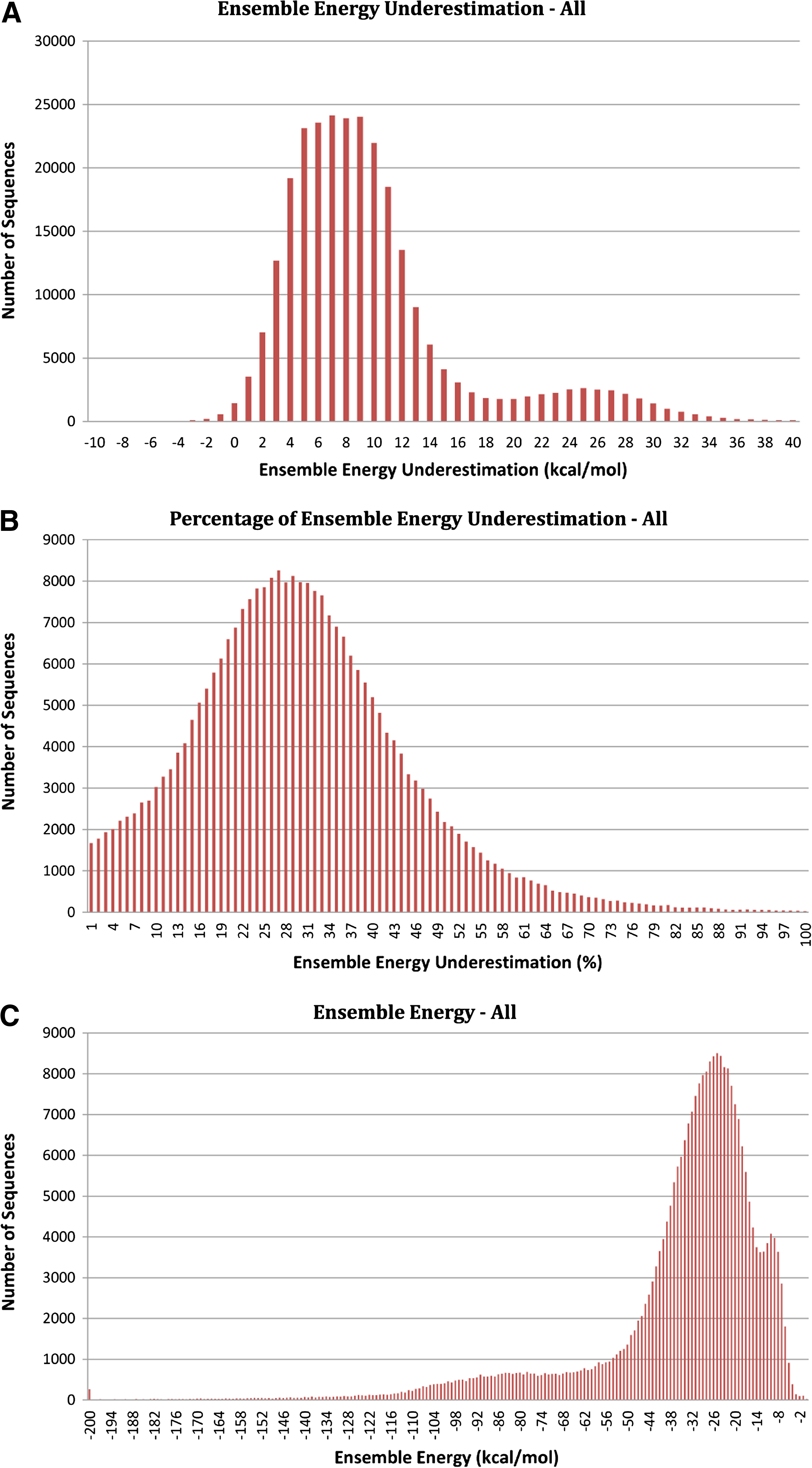
We implemented the upper bound algorithm in our piRNA package (Chitsaz et al., 2009). To test the overestimation of partition function and also the number of samples needed for the algorithm to converge, we randomly selected 273,512 RNA sequences from Rfam 11.0 database (Gardner et al., 2011; Griffiths-Jones et al., 2003) and computed the upper bounds. Since the partition functions are often large numbers, we report the ensemble energies. The ensemble energy is proportional to the minus log of the partition function and an overestimation of the partition function becomes an underestimation of the ensemble energy. Figure 1 depicts the results of our experiment. The top plot shows the histogram of ensemble energy underestimation calculated by −RT log Q + RT log Q_ub. The middle plot shows the histogram of ensemble energy underestimation percentage calculated from the ratio log Q_ub/log Q − 1. This plot shows that for a vast majority of cases this ratio is below 40%. The bottom plot depicts the distribution of ensemble energy −RT log Q in the input dataset. Although this distribution exhibits multiple peaks, the middle distribution, which is the underestimation percentage, has a unimodal behavior. Out of 273,512 RNAs, for 249,622 of them the underestimation is less than 50% of their ensemble energy, and for about half of the sequences (148,762) this difference is smaller than 30%. The number of sequences for which this difference is negative is 2,356, which is less than 1% of the total number of RNAs.

OPEN IN VIEWER

FIG. 1.

Histograms of (A) ensemble energy underestimation −RT log Q + RT log Q_ub for all 273,512 sequences in our dataset, (B) percentage of ensemble energy underestimation log Q_ub / logQ − 1, and (C) ensemble energy −RT log Q in the input dataset.

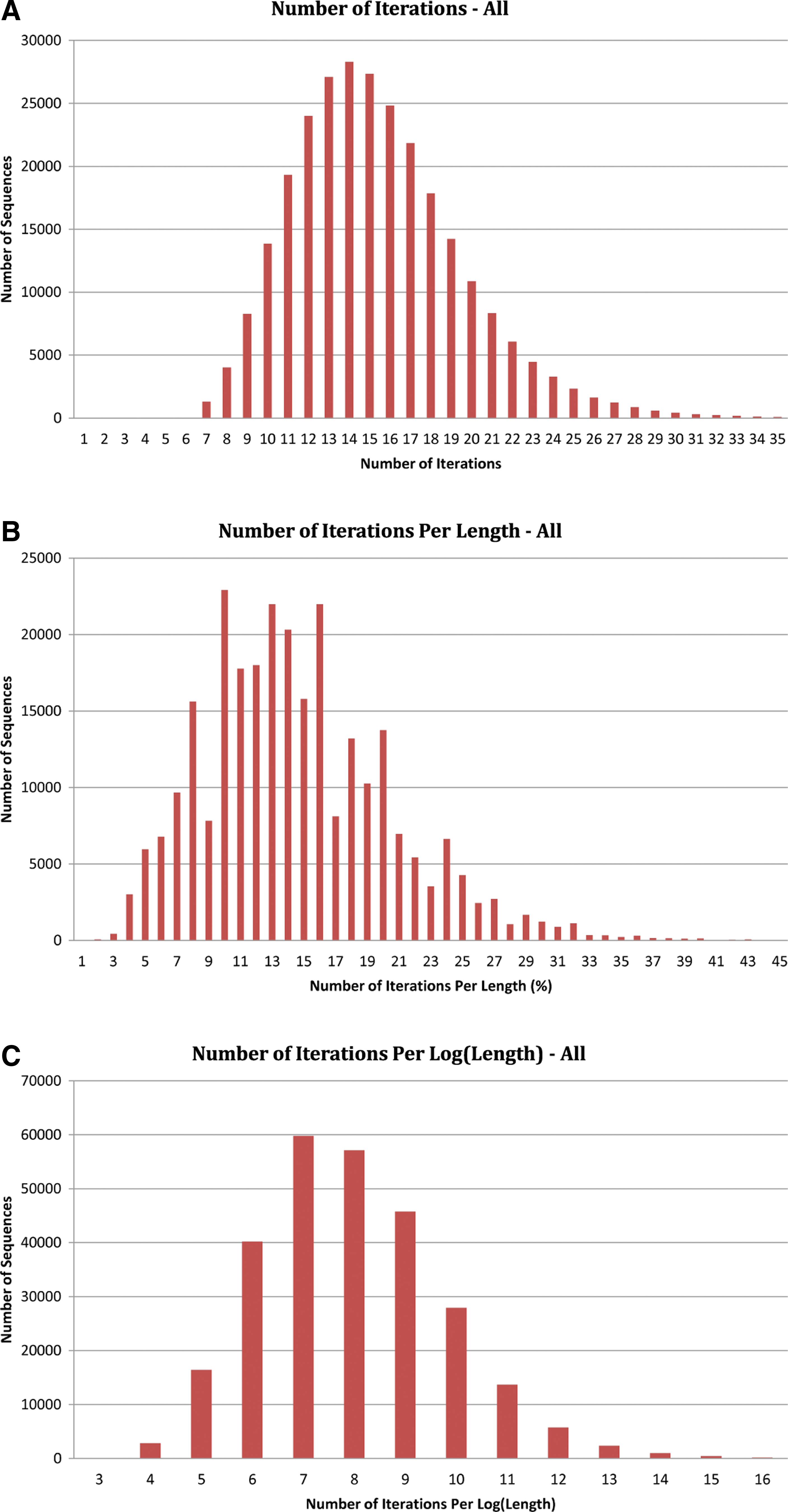
Figure 2 shows the performance of our algorithm. Figure 2A is the histogram of the number of samples ℓ (iterations) needed for the algorithm to converge. Figure 2B and C show the histogram of the number of iterations per input size and per the log of input size. The vast majority of sequences required less than 15% of their length iterations to converge. The number of iterations starts with 7 and almost all the sequences need less than 40 samples. 243,119 or 89% of RNAs need no more than 20 iterations, and for more than half of the sequences (153,515), the experiment has been done with less than 15 iterations. Therefore, at most 40 iterations are enough for different Rfam RNAs with different lengths. The number of iterations per length ratio for most of the sequences is less than 30%. For 90% of the RNAs in this dataset, this number is between 7% and 25%. Clearly the relation between length and the number of iterations is not linear, and upper bounds for different RNAs with the same length require a different number of iterations. Recall that the space complexity of our algorithm is the same as that of sparse minimum free energy prediction. Therefore, our algorithm is both fast and space efficient in practice.

OPEN IN VIEWER

FIG. 2.

Histograms of (A) number of iterations ℓ needed for all sequences in our dataset, (B) number of iterations as a percentage of the input sequence length, and (C) number of iterations per the log of the input sequence length.

6. Conclusion

We gave a fast algorithm, based on the recent algorithm of Hazan and Jaakkola (2012), to iteratively compute an upper bound on the partition function of nucleic acids by perturbing energy. Our upper bound algorithm uses a fast minimum free energy prediction in each iteration. Our algorithm preserves the properties on which sparsification methods rely; therefore, we minimally modified sparse folding algorithms (Backofen et al., 2011; Mohl et al., 2010; Salari et al., 2010) to obtain the required fast minimum free energy prediction.

For the lower bound, one can trivially use the single term corresponding to the minimum free energy. The lower bound algorithm of Hazan and Jaakkola (2012) requires modification in order to be applicable to our problem. We leave such accurate lower-bound algorithms for future work.